Towards soliton solutions of a perturbed sine-Gordon

equation

A. D’Anna¹, M. De Angelis¹, G. Fiore 

Abstract: We give arguments for the existence of exact travelling-wave solutions, of old (in particular solitonic) and new type, of a perturbed sine-Gordon equation on the real line or on the circle, and classify them. The perturbation of the equation consists of a constant forcing term and a linear dissipative term. Such solutions are allowed exactly by the energy balance of these terms, and can be observed experimentally e.g. in the Josephson effect in the theory of superconductors, which is one of the physical phenomena described by the equation.

Preprint 05-30 Dip. Matematica e Applicazioni, Univ. “Federico II”, Napoli
DSF/13-2005

1 Introduction

The “perturbed” sine-Gordon equation

$$\varphi_{tt}-\varphi_{xx}+\sin\varphi+\alpha\varphi_{t}+\gamma=0,\qquad x\in{\mathbb{R}},$$ (1)

($\alpha\geq 0,\gamma\in{\mathbb{R}}$ are constants) has been used to describe with a good approximation a number of interesting physical phenomena, notably Josephson effect in the theory of superconductors [9], or more recently also the propagation of localized magnetohydrodynamic modes in plasma physics [20]. The last two terms are respectively a dissipative and a forcing one; the (unperturbed) sine-Gordon equation is obtained by setting them equal to zero.

In the Josephson effect $\varphi(x,t)$ is the phase difference of the macroscopic quantum wave-functions describing the Bose-Einstein condensates of Cooper pairs in two superconductors separated by a very thin, narrow and long dielectric (a socalled “Josephson junction”). The $\gamma$ term is the (external) socalled “bias current”, providing energy to the system, whereas the dissipative term $\alpha\varphi_{t}$ is due to Joule effect of the residual normal current across the junction, due to electrons not paired in Cooper pairs. Additional terms can be added to describe additional features, e.g. a term like $\sigma\varphi_{x}$ would approximately describe [15] the Josephson effect in a junction with a linearly varying (albeit very small) breadth, whereas a dissipative term like $-\varepsilon\varphi_{xxt}$ would take into account (see e.g. [2]) the effect of the residual normal current along the junction. We plan to address the latter, third order equation elsewhere, exploiting our results [5, 4] about equations involving the differential operator $-\varepsilon\partial_{x}^{2}\partial_{t}+\partial_{t}^{2}-\partial_{x}^{2}$.

Among the solutions of the sine-Gordon equation the solitonic ones are particularly important, in that they describe stable waves propagating along the $x$-line. There are strong experimental (see e.g. [2] for the Josephson effect), numerical [8, 14] and analytical [7, 13] indications that solutions of this kind are deformed, but survive in the perturbed case; nevertheless, up to our knowledge there is no rigorous proof of this. The analytical indications are obtained within the by now standard perturbative method [10, 16, 11, 12] based on modulations of the unperturbed (multi)soliton solutions with slowly varying parameters (tipically velocity, space/time phases, etc. ) and small radiation components. (This is inspired by the Inverse Scattering Method). The Ansatz for the approximate one-(anti)soliton solution reads

$$\varphi(x,t)=\hat{g}_{0}\Big{(}x\!-\!x_{0}(t)\!-\!\tilde{v}(t)t\Big{)}\!+\!\epsilon\varphi_{1}(x,t)\!+\!...$$

where $\varphi_{0}(x,t):=\hat{g}_{0}(x-vt)$ is one of the unperturbed (anti)soliton solutions given below in (14), whereas the slowly varying $x_{0}(t),\tilde{v}(t)$ and the perturbative “radiative” corrections $\epsilon\varphi_{1}(x,t)+...$ have to be computed perturbatively in terms of the perturbation $\epsilon f$ of the sine-Gordon equation (in the present case one may choose $\epsilon=\gamma$ and $\epsilon f=+\alpha\varphi_{t}+\gamma$). One finds in particular approximate solutions with constant velocity

$$\tilde{v}(t)\equiv v_{\infty}:=\pm[1+(4\alpha/\pi\gamma)^{2}]^{-\frac{1}{2}}$$ (2)

which are characterized by a power balance between the dissipative term $\alpha\varphi_{t}$ and the external force term $\gamma$. They are interpreted as approximating expected exact (anti)soliton solution. The experimentally observed velocity is consistent with the value $v_{\infty}$ within present experimental errors.

The purpose of this work is to give non-perturbative arguments for the existence of exact travelling-wave (in particular solitonic) solutions of the above equation on the real line or on the circle, and a preliminary classification of them. Our approach is less ambitious, in that it is based on pushing forward the study of the ordinary differential equation which is obtained by replacing in the equation (1) the standard travelling-wave Ansatz

$$\varphi(x,t)=\tilde{g}(\tilde{\xi})=\tilde{g}(x-vt)$$ (3)

(here and in the sequel $\tilde{\xi}:=x-vt$), and therefore cannot be applied to multisolitonic solutions. The ordinary differential equation is the same as the one describing the motion along a line of a particle subject to a “washboard” potential and immersed in a linearly viscous fluid, and therefore the problem is essentially reduced to studying this simpler mechanical analog where $\tilde{\xi}$ plays the role of ‘time’. After reviewing (section 2) travelling-wave solutions of the sine-Gordon equation in section 3 we classify the possible solutions of the latter, identifying those having bounded energy density at infinity and possibly yielding stable solutions for (1); the main results are collected in Proposition 1. The actual existence of such solutions is strongly suggested by our physical expectations on the mentioned particle mechanical analog and will be proved elsewhere [6], together with some general properties of these solutions (there we will also provide an alternative perturbative scheme for their determination). Among the solutions there are: those yielding solitonic solutions for (1), which are characterized by their going to two neighbouring local maxima of the potential energy of the particle as $\tilde{\xi}\to\pm\infty$; those yielding “array of (anti)solitons” solutions; those yielding “half-array of (anti)solitons” solutions. The occurrence of the latter is a new phenomenon, with no counterpart in the pure sine-Gordon case. Also, contrary to the unperturbed case, the propagation velocity $v$ of the soliton turns out to be not a free parameter, but a function of $\alpha,\gamma$, which coincides [6], at lowest order in $\gamma$, with (2).

1.1 Preliminary considerations:

Given a solution one can find a two-parameter family with infinitely many others by space or time translations; therefore, for each family it suffices to give just one representative element.

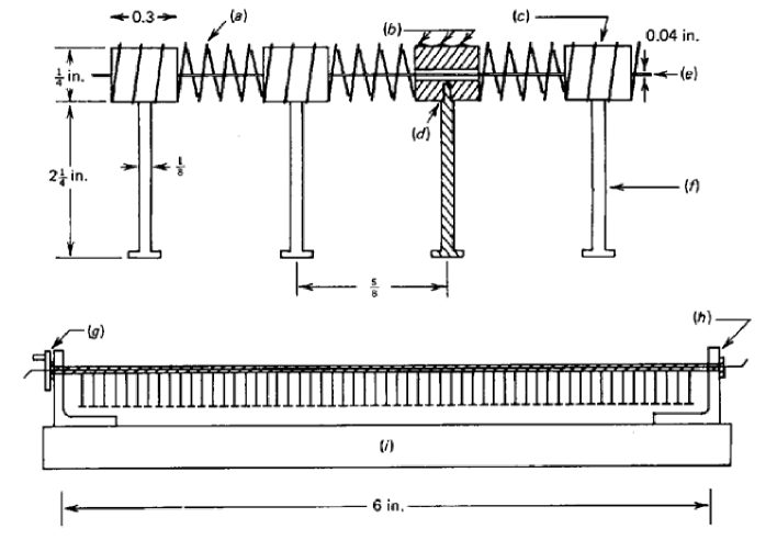
Figure 1: Mechanical model for the sine-Gordon equation. (a) Spring, (b) dolder, (c) brass, (d) tap and thread, (e) wire, (f) nail, (g) and (h) ball bearings, (i) base (After A. C. Scott [19], courtesy of A. Barone, see [2])

A system obeying the sine-Gordon equation can be modelled [19] by the discretized mechanical analog in fig. 1, namely a chain of heavy pendula constrained to rotate around a horizontal axis and coupled to each other through a spring applying an elastic torque; one can model also the dissipative term $-\alpha\varphi_{t}$ of (1) by immersing the pendula in a linearly viscous fluid, and the forcing term $\gamma$ by assuming that there is a uniform friction between the pendula and the horizontal axis, and that the latter rotates with constant velocity.

The constant solutions of (1) are $\varphi(x,t)\equiv-\sin^{-1}\gamma\!+\!2\pi k$ and $\varphi(x,t)\equiv\sin^{-1}\gamma\!+\!(2k\!+\!1)\pi$. The former are stable, the latter unstable. To see this one just needs to note that they yield respectively local minima and maxima of the energy density

$$h:=\frac{\varphi_{t}^{2}}{2}+\frac{\varphi_{x}^{2}}{2}+\gamma\varphi-\cos\varphi+K.$$ (4)

This is visualized in the mechanical analog in fig. 1 respectively by configurations with all pendula hanging down or standing up. We choose the free constant $K\in{\mathbb{R}}$ so that it gives a zero energy density at one (particular) stable constant solution, $\varphi(x,t)\equiv-\sin^{-1}\gamma$: then $K=\sqrt{1-\gamma^{2}}+\gamma\sin^{-1}\gamma$. In general, as a consequence of (1) $h$ fulfills the equation

$$\partial_{t}h-\partial_{x}j=-\alpha\varphi_{t}^{2}.$$ (5)

where we have introduced the energy current density $j:=\varphi_{x}\varphi_{t}$. If $\alpha=0$ this is a continuity equation. The negative sign at the rhs shows the dissipative character of the time derivative term in (1) if $\alpha>0$.

Our working definition of a (multi)solitonic solution $\varphi$ is: A) It is a stable solution which significantly differs from some minima of the energy density $h$ only in some localized regions; this means that mod. $2\pi$ it must be

$$\lim\limits_{x\to-\infty}\varphi(x,t)=-\sin^{-1}\!\gamma,\qquad\lim\limits_{x\to+\infty}\varphi(x,t)=-\sin^{-1}\!\gamma+2n\pi\qquad$$ (6)

with $n\in{\mathbb{Z}}$. Moreover, as usual we require that: B) In the far past $\varphi$ is approximately a superposition of single solitons, antisolitons (and possibly breathers), which in the far future emerge from collisions again with the same shape and velocities with which they entered [however, in this work we shall only deal with single (anti)solitons]. As we shall recall below, one-soliton and one-antisoliton solutions are characterized by $n=1,-1$ respectively [whereas the static stable and constant solution $\varphi(x,t)\equiv\sin^{-1}\gamma\mbox{ (mod }2\pi)$ correspond to $n=0$]. In the mentioned mechanical analog the one-(anti)soliton solution describes a localized twisting of the pendula chain by $2\pi$ (anti)clockwise, as depicted in figure 3 (a), moving with constant velocity. The above condition yields an energy density $h$ (rapidly) going to $0,2n\pi\gamma$ respectively as $x\to-\infty,\infty$; only if $\gamma=0$, i.e. if the values of the potential energy at all the minima coincide, the potential energy $h$ vanishes at both $x\to-\infty,\infty$, and one recovers the standard definition of solitons.

Although $n\neq 0$ makes the total Hamiltonian

$$H:=\int\limits_{-\infty}^{+\infty}h(x,t)dx$$ (7)

divergent, it gives a well-defined, non-positive time-derivative

$$\dot{H}=-\int\limits^{\infty}_{-\infty}\alpha\varphi_{t}^{2}\leq 0,$$

as a result of integration of (5). The effect of $\gamma\neq 0$ is to make the values of the energy potential at any two minima different; this leaves room for an indefinite compensation of the dissipative power loss by a falling down in the total potential energy, and so may account for solutions not being damped to constants as $t\to\infty$.

Without loss of generality we can assume $\gamma\geq 0$. If originally this is not the case, one just needs to replace $\varphi\to-\varphi$. If $\gamma>1$ no solutions $\varphi$ having finite limits and vanishing derivatives for $x\to\pm\infty$ can exist, in particular no static solutions. If $\gamma=1$ the only static solution $\varphi$ having for $x\to\pm\infty$ finite limits and vanishing derivatives is $\varphi\equiv-\pi/2\mbox{ (mod }2\pi)$, which however is unstable. In the sequel we shall assume $0\leq\gamma<1$.

2 The sine-Gordon equation

Before going on, let us recall [1, 3] what happens in the case $\gamma=0=\alpha$. The sine-Gordon equation is

$$\varphi_{tt}-\varphi_{xx}+\sin\varphi=0,\qquad\qquad x\in{\mathbb{R}}.$$ (8)

The associated Hamiltonan (a conserved quantity) is

$$H_{0}:=\int\limits_{-\infty}^{+\infty}\left(\frac{\varphi_{t}^{2}}{2}+\frac{\varphi_{x}^{2}}{2}-\cos\varphi+1\right)dx.$$ (9)

Let $\tilde{\xi}:=x-vt$. One looks for travelling-wave solutions of (8), namely for solutions with a ‘fixed-profile’ Ansatz (3). As the time $t$ flows the profile of $\tilde{g}$ will move to the right/left according to a positive/negative sign of $v$. Replacing the Ansatz in the sine-Gordon equation one finds for $\tilde{g}$ the equation $(v^{2}-1)\tilde{g}^{\prime\prime}+\sin\tilde{g}=0$. If $v^{2}=1$ the equation admits only the (stable or unstable) static solutions $\varphi(x,t)=\tilde{g}(\tilde{\xi})\equiv 0,\pi$ (mod $2\pi$). Otherwise it can be rewritten in the form

$$g^{\prime\prime}+\sin g=0,$$ (10)

where

$$\xi=\sigma\frac{\tilde{\xi}}{\sqrt{|v^{2}\!-\!1|}},\qquad g(\xi):=\eta\cases{\tilde{g}(\xi)\>\>\>\mbox{ if }v^{2}\geq 1\cr\tilde{g}(\xi)\!-\!\pi\>\>\>\mbox{ if }v^{2}<1,}$$ (11)

where $\eta,\sigma=\pm 1$ are arbitrary signs. This is the equation of motion w.r.t. the ‘time’ $\xi$ of a pendulum ($g$ being the deviation angle from the stable equilibrium position), or equivalently of a particle in a sinusoidal “energy potential” $U=-\cos g$. Multiplying the equation by $g^{\prime}$ one finds the “mechanical energy of the pendulum” integral of motion e

$$\qquad\frac{d}{d\xi}\left[\frac{g^{\prime}{}^{2}}{2}\!-\!\cos g\right]=0\qquad\Rightarrow\qquad\mbox{\rm e}:=\frac{g^{\prime}{}^{2}}{2}\!+\!U=\mbox{const}.$$ (12)

By definition $\mbox{\rm e}\geq-1$. The above implies

$$\pm dg\frac{1}{\sqrt{2(\mbox{\rm e}\!+\!\cos g)}}=d\xi.$$

The latter equation can be immediately integrated out, giving $\xi=\xi(g)$. The final step is the inversion of this function in disjoint intervals, which will give $g=g(\xi)$, and patching the intervals.

Figure 2: The potential energy $U$

According to the choice of $\mbox{\rm e},v$ one obtains different kinds of solutions. Plotting the potential energy (Fig. 2) helps us get an immediate qualitative understanding of them.

1. If $\mbox{\rm e}=\mbox{\rm e}_{0}:=-1$ then necessarily $g(\xi)\equiv 0\,(\mbox{mod}2\pi)$. This corresponds to the constant solutions

   $$\varphi^{s}(x,t)\equiv 0\,(\mbox{mod}2\pi)\qquad\qquad\varphi^{u}(x,t)\equiv\pi\,(\mbox{mod}2\pi)$$ (13)

   respectively if $v^{2}>1$ and $v^{2}<1$. The former (resp. latter) is clearly stable (resp. unstable) because it corresponds to all pendula hanging downwards (resp. standing upwards) in the model of fig. 1. The same constant solutions arise from considering the constant $g=(2k+1)\pi$, corresponding to $\mbox{\rm e}=\mbox{\rm e}_{2}=1$.

2. If $-1<\mbox{\rm e}<1$ ($\mbox{\rm e}=\mbox{\rm e}_{1}$ in Fig. 2) then the corresponding solution $\bar{g}_{0}(\xi;\mbox{\rm e})$ can be written in terms of elliptic functions and describes the motion of a particle confined in an interval contained in $]-\pi,\pi[$ and oscillating around $g=0$ ($\mbox{mod}2\pi$) with some period $\Xi_{p}(\mbox{\rm e})$. For $\varphi$, this translates into a periodic oscillating wave travelling with velocity $v$: If $v^{2}>1$ then $\varphi$ oscillates around the stable equilibrium solution $\varphi^{s}\equiv 0$ and describes a “plasma wave”, see fig. 3 (c), (d); if $v^{2}<1$ then $\varphi$ oscillates around the unstable equilibrium solution $\varphi^{u}\equiv\pi$. Both kinds of $\varphi$ are however unstable [18, 1, 3].

3. If $\mbox{\rm e}=\mbox{\rm e}_{2}=1$, beside the constant solution yielding (13), there are in addition the solutions

   $$\hat{g}_{0}(\pm\xi)=4\tan^{-1}\left[\exp(\pm\xi)\right]-\pi.$$

   Mod $2\pi$, $\hat{g}_{0}(\xi)\to\pm\pi$ as $\xi\to\pm\infty$: the particle, confined in the interval $-\pi\!<\!g\!<\!\pi$, starts at ‘time’ $\xi=-\infty$ from one top of the energy potential and reaches the other one at $\xi=\infty$. Mod. $2\pi$, they translate into the following solutions of the original problem (8)

   $$\varphi_{0}^{\pm}(x,t;v)=4\tan^{-1}\left\{\exp\left[\pm\frac{x-vt}{\sqrt{v^{2}\!-\!1}}\right]\right\}-\pi\qquad\mbox{ if }v^{2}>1,\qquad$$

   $$\hat{\varphi}_{0}^{\pm}(x,t;v)=4\tan^{-1}\left\{\exp\left[\pm\frac{x-vt}{\sqrt{1\!-\!v^{2}}}\right]\right\}\qquad\mbox{ if }v^{2}<1.\qquad$$ (14)

   Both families represent solutions (rotating clockwise or anti-clockwise according to the sign $\pm$) with localized region of variation of $\varphi$ and travelling with velocity $v$. The first families are clearly unstable because they describe solutions of the model of fig. 1 where all pendula stand upwards except in the small moving region where they twist once around the axis; their values of the total mechanical energy $H$ are infinite. The second families are stable [18, 1, 3], as it can be expected from the fact that they describe solutions of the mechanical model of fig. 1 where all pendula hang downwards except in the small moving region where they twist once around the axis, see fig. 3 (a); their values of the total mechanical energy $H$ are finite. They represent respectively a soliton ($\varphi_{0}^{+}$) and an antisoliton ($\varphi_{0}^{-}$) travelling with velocity $v$. Note that they fulfill (6) with $n=\pm 1$. For $v=0$ we have a static (anti)soliton.

4. If $\mbox{\rm e}=\mbox{\rm e}_{3}>1$ (see Fig. 2) then the corresponding solution $\check{g}_{0}(\pm\xi;\mbox{\rm e})$ describes a particle moving towards the right and the left respectively, ‘for ever’, since it has a sufficient energy to overcome the tops of the energy potential. Moreover, its kinetic energy and velocity are periodic with some period $\Xi_{0}(\mbox{\rm e})$, (with $\Xi_{0}\to\infty$ as $\mbox{\rm e}\downarrow 1$). This means, for any $\xi\in{\mathbb{R}}$,

   $$\check{g}_{0}(\xi+\Xi_{0};\mbox{\rm e})=\check{g}_{0}(\xi;\mbox{\rm e})+2\pi,$$ (15)

   i.e. $g(\xi)$ is the sum of a linear and of a periodic function. Again, the corresponding solutions of the original problem (8) are unstable or [18, 1, 3] stable according to $v^{2}\!>\!1$ or $v^{2}\!<\!1$, because they correspond to ‘most’ pendula up or down in the model of fig. 1. The stable solutions ($v^{2}\!<\!1$) $\check{\varphi}_{0}^{\pm}$ describe evenly spaced “arrays of solitons and antisolitons”, travelling with velocity $v$, see fig. 3 (b).

No $n$ with $|n|>1$ is allowed for travelling wave solutions fulfilling (6).

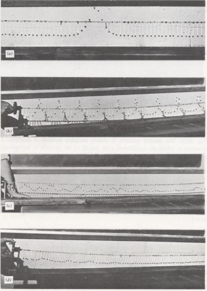
Figure 3: Photographs of the mechanical model of fig. 1: (a) single soliton solution, (b) evenly spaced array of solitons, large (c) and small (d) amplitude plasma wave solutions (After A. C. Scott [19], courtesy of A. Barone, see [2])

3 Adding the forcing and the first order dissipative terms in the equation

We still adopt the Ansatz (3) for the solutions of (1) and ask how the classes of solutions found in the preceding section are deformed. We are interested in stable solutions $\varphi$ with bounded derivatives for $x\to\pm\infty$. Having in mind the mechanical analog of the chain of pendula, it is natural to expect that solitonic solutions will survive perturbation: if we just smoothly switch $\gamma$ then even the static soliton will start to move and gradually accelerate; if we now also switch $\alpha$, we expect that its propagation will approach a steady regime in which dissipation and forcing balance each other. We are actually going to see that not only the solitonic, but also the other classes of solutions found in the previous section survive perturbation whenever a compensation of the forcing term $\gamma$ with the dissipation term in $\alpha$ can take place.

Replacing the Ansatz (3) in (1) we find the equation

$$(v^{2}-1)\tilde{g}^{\prime\prime}-\alpha v\tilde{g}^{\prime}+\sin\tilde{g}+\gamma=0,\qquad x\in{\mathbb{R}}.$$ (16)

If $v=\pm 1$ the second order derivative in (16) disappears and we get

$$\pm\,\alpha\tilde{g}^{\prime}=(\sin\tilde{g}+\gamma).$$

Unless $\tilde{g}$ is constant (and therefore equal to $-\sin^{-1}\gamma$ or $\pi\!+\!\sin^{-1}\gamma$) then there exists a $\tilde{\xi}_{0}$ such that $\tilde{g}^{\prime}(\tilde{\xi}_{0})\neq 0$ and $\tilde{g}_{0}:=\tilde{g}(\tilde{\xi}_{0})\neq-\sin^{-1}\gamma,\pi+\sin^{-1}\gamma$. Integrating in a neighbourhood of $\tilde{\xi}_{0}$ one finds

$$\tilde{\xi}-\tilde{\xi}_{0}=\int\limits^{\tilde{\xi}}_{\tilde{\xi}_{0}}d\tilde{\xi}^{\prime}=\pm\alpha\int\limits^{\tilde{g}}_{\tilde{g}_{0}}\frac{dz}{\sin z+\gamma}.$$

As $\tilde{g}$ approaches respectively $-\sin^{-1}\gamma$ or $\pi\!+\!\sin^{-1}\gamma$ (mod. $2\pi$) the denominator goes to zero linearly while keeping the same sign, and therefore the integral diverges logarithmically, implying that the corresponding time $\tilde{\xi}$ goes respectively to $\pm\infty$ (or viceversa). The corresponding solution $\varphi$ for (1) is unstable, therefore is not interesting for our scopes, because: it yields a maximum of the energy density $h$ as either $\tilde{\xi}\to\infty$, or $\tilde{\xi}\to-\infty$, i.e. there it corresponds to all pendula standing upwards (while hanging downwards resp. as $\tilde{\xi}\to-\infty$ or $\tilde{\xi}\to\infty$).

If $v^{2}\neq 1$ we perform the redefinitions [compare with (11)]

$$\begin{array}[]{ll}\xi:=-\mbox{sign}(v)\frac{\tilde{\xi}}{\sqrt{v^{2}\!-\!1}}&g(\xi)\!:=\!-\tilde{g}(\xi)\>\>\>\mbox{ if }v^{2}\!>\!1,\\[8.0pt] \xi\!:=\!\mbox{sign}(v)\frac{\tilde{\xi}}{\sqrt{1\!-\!v^{2}}}&g(\xi)\!:=\!\tilde{g}(\xi)\!-\!\pi\>\>\>\mbox{ if }v^{2}\!<\!1,\\[8.0pt] \xi\!:=\!\tilde{\xi}\!=\!x&g(\xi)\!:=\!\tilde{g}(\xi)-\pi\>\>\>\mbox{ if }v=0;\end{array}\qquad$$ (17)

we obtain

$$g^{\prime\prime}+\mu g^{\prime}+U_{g}(g)=0,\qquad\xi\in{\mathbb{R}},$$ (18)

which can be regarded as the 1-dimensional equation of motion w.r.t. the ‘time’ $\xi$ of a particle with unit mass, a ‘potential energy’ $U(g)=-(\cos g+\gamma g)$ (see Fig. 4) and a viscous force with viscosity coefficient

$$\mu:=\frac{\alpha}{\sqrt{|v^{-2}-1|}}$$ (19)

[in other words, in the equation $\alpha,v$ appear only through their combination (19)]. One immediately finds that the ‘mechanical energy’ is not ‘time’ independent, but decreases according to

$$\mbox{\rm e}^{\prime}=-\mu g^{\prime}{}^{2}\leq 0$$ (20)

Figure 4: The potential energy $U$ for $\gamma=.1$ and three mechanical-energy levels for $\mu=0$ (no dissipation).

$U$ admits local minima (resp. maxima) in the points

$$g_{k}^{m}:=\sin^{-1}\gamma\!+\!2k\pi\qquad\qquad(\mbox{resp. }g_{k}^{M}:=\pi\!-\!\sin^{-1}\gamma\!+\!2k\pi),$$

and their corresponding values of $U$ are

$$U(g_{k}^{m})=-\left[\gamma(\sin^{-1}\gamma+2k\pi)+\sqrt{1-\gamma^{2}}\right],$$

$$U(g_{k}^{M})=-\left[\gamma\left(-\sin^{-1}\gamma+(2k\!+\!1)\pi\right)-\sqrt{1-\gamma^{2}}\right];$$

they linearly decrease with $k$.

We have to look for solutions of (18) such that $g^{\prime}$ is bounded all over ${\mathbb{R}}$. Multiplying (18) by $g^{\prime}$ and integrating over an interval $[\xi,\bar{\xi}]$ we find

$$\qquad\frac{1}{2}g^{\prime}{}^{2}(\xi)=\frac{1}{2}g^{\prime}{}^{2}(\bar{\xi})+\left[U\Big{(}g(\bar{\xi})\Big{)}\!-\!U\Big{(}g(\xi)\Big{)}\right]+\mu\int\limits^{\bar{\xi}}_{\xi}g^{\prime}{}^{2}(\xi^{\prime})d\xi^{\prime}.$$ (21)

1. The constant (in $\xi$) solutions corresponding to the local minima, maxima of the potential energy become $g(\xi)\equiv g_{k}^{m}$, $g(\xi)\equiv g_{k}^{M}$. The latter are the solutions for which there exists a $\bar{\xi}$ such that $g(\bar{\xi})=g_{k}^{M}$ and $g^{\prime}(\bar{\xi})=0$ (actually this happens for all $\bar{\xi}\in{\mathbb{R}}$). The particular ones $g(\xi)\equiv g_{0}^{m}$, $g(\xi)\equiv g_{0}^{M}$ correspond to the energy levels ${\rm e}={\rm e}_{0}:=U(g_{0}^{m})$, ${\rm e}={\rm e}_{2}:=U(g_{0}^{M})$ in Fig. 4. These solutions translate into the following constant solutions for the original problem: (mod. $2\pi$)

   $$\qquad\varphi^{s}(x,t)\!\equiv\!-\!\sin^{-1}\!\gamma\qquad\varphi^{u}(x,t)\!\equiv\!\sin^{-1}\!\gamma\!+\!\pi$$ (22)

   (the former are stable, the latter unstable).

2. If there exists some ‘time’ $\bar{\xi}$ such that $g(\bar{\xi})=g_{k}^{M}$ and $g^{\prime}(\bar{\xi})<0$ (particle located at some maximum of $U$ and moving leftwards), then necessarily

   $$g(\xi)\stackrel{{\scriptstyle\xi\to-\infty}}{{\longrightarrow}}\infty,\qquad\qquad\qquad g^{\prime}(\xi)\stackrel{{\scriptstyle\xi\to-\infty}}{{\longrightarrow}}-\infty,$$

   so for our scopes we can readily exclude this case.

3. If there exists no ‘time’ $\bar{\xi}$ such that $g(\bar{\xi})$ is a local maximum of $U$, then necessarily the motion is confined in some interval $]g^{M}_{k\!-\!1},g^{M}_{k}[$ and $|g^{\prime}(\xi)|$ by (21) keeps bounded. We have already treated the constant $g(\xi)\equiv g_{k}^{m}$ solutions, so let us consider the others.

   If $\mu=0$ (note that this is the case not only if $\alpha=0$, but also if $\alpha>0$ and $v=0$, i.e. for a static $\varphi$) and:

   1. ${\rm e}<U(g_{k}^{M})$, then $g(\xi)$ will be periodic, oscillating ‘for ever’ around $g_{k}^{m}$; in fig. 4 this corresponds to e=e₁ with $g\in]g^{M}_{-1},g^{M}_{0}[$. The corresponding solutions $\varphi$ of the original problem will describe again unstable oscillations around the unstable equilibrium position if $v^{2}<1$, and unstable ‘plasma wave’ oscillations around the stable equilibrium position if $v^{2}>1$.

   2. ${\rm e}=U(g_{k}^{M})$ , then $g(\xi)\to g_{k}^{M}$ for both $\xi\to\pm\infty$; in fig. 4 this corresponds to e=e₂ with $g\in]g^{M}_{-1},g^{M}_{0}[$. If $v^{2}>1$ this will yield again an unstable solution $\varphi$, because the latter corresponds to all the pendula standing upwards at infinity, whereas if $v^{2}<1$ this will yield a new type of solution $\varphi$ of the original problem, a kind of rigidly bounded soliton-antisoliton pair. Whether this is stable or not should be investigated.

   If $\mu$ (and therefore $\alpha$) is positive, then necessarily

   $$g^{\prime}(\xi)\stackrel{{\scriptstyle\xi\to-\infty}}{{\longrightarrow}}0,\qquad\qquad g^{\prime}(\xi)\stackrel{{\scriptstyle\xi\to\infty}}{{\longrightarrow}}0.$$

   As a consequence, using the equation of motion (18), as $\xi\to\pm\infty$ $g$ must go to one of the following values: $g^{M}_{k\!-\!1},g_{k}^{m},g_{k}^{M}$. If in addition there exists some ‘time’ $\bar{\xi}$ such that $g^{\prime}(\bar{\xi})<0$ (particle moving leftwards), then necessarily

   $$g(\xi)\stackrel{{\scriptstyle\xi\to-\infty}}{{\longrightarrow}}g_{k}^{M}\mbox{ or }g^{M}_{k\!-\!1},\qquad\qquad\qquad g(\xi)\stackrel{{\scriptstyle\xi\to\infty}}{{\longrightarrow}}g_{k}^{m}.$$

   Such a $g$ translates into an unstable solution $\varphi$ of the original problem, because it yields a maximum of the energy density $h$, i.e. it corresponds to all pendula standing upwards, for either $\xi\to\infty$ or $\xi\to-\infty$ [depending which of the two possible definitions of $g$ in (11) is adopted].

   We are left with the last, most interesting possibility, namely a solution $\hat{g}$ such that

   $$\hat{g}(\xi)\stackrel{{\scriptstyle\xi\to-\infty}}{{\longrightarrow}}g^{M}_{k\!-\!1}\qquad\qquad\qquad\hat{g}(\xi)\stackrel{{\scriptstyle\xi\to\infty}}{{\longrightarrow}}g_{k}^{M}$$ (23)

   and $\hat{g}^{\prime}(\xi)>0$ for all $\xi$. This will translate into an unstable solution $\varphi$ (almost all pendula standing upwards) if $v^{2}>1$ [see (11)], candidate stable solutions $\hat{\varphi}^{\pm}$ (almost all pendula hanging downwards) if $v^{2}<1$. The latter will describe the propagation of an (anti)soliton with velocity $v$ [fig. 3 (a)]. That such a solution exists can be argued as follows. Impose just (23)₁. Consider first the case $\mu=0$: the mechanical energy of the particle has the constant value ${\rm e}=U(g^{M}_{k-1})$, the corresponding solution will reach and overcome $g_{k}^{M}$ after a finite time. Second, it is easily expected and not difficult to show [6] that for sufficiently large $\mu$ the corresponding solution will never reach $g_{k}^{M}$, but rather invert its motion at some $g<g_{k}^{M}$ and go to $g_{k}^{m}$ as $\xi\to\infty$. By continuity, we expect that there exists a special value $\hat{\mu}(\gamma)$ such that the corresponding solution $\hat{g}$ fulfills also (23)₂. As an immediate consequence of the definition of $\mu$ the propagation velocity $v$ (for $v^{2}<1$) is determined [see formula (27) below]. One can determine $\hat{\mu}(\gamma)$ perturbatively in $\gamma$ [6]; at lowest order one finds $\hat{\mu}(\gamma)=\pi\gamma/4+...$, which gives a $v$ coinciding with (2), but higher orders will correct the latter formula.

4. It remains to consider the cases that there exists some ‘time’ $\xi_{k}$ such that $g(\xi_{k})=g_{k}^{M}$ (particle located at some maximum of $U$), but $g^{\prime}(\xi_{k})>0$ (particle moving rightwards) at all such ‘times’. Then necessarily $g^{\prime}(\xi)>0$ for all (finite) $\xi<\xi_{k}$. As a consequence, it will be

   $$\begin{array}[]{llll}\mbox{either }&g(\xi)\stackrel{{\scriptstyle\xi\to-\infty}}{{\longrightarrow}}-\infty&\mbox{and}&g(\xi)\stackrel{{\scriptstyle\xi\to\infty}}{{\longrightarrow}}\infty\\[8.0pt] \mbox{or }&g(\xi)\stackrel{{\scriptstyle\xi\to-\infty}}{{\longrightarrow}}g^{M}_{l}&\mbox{and}&g(\xi)\stackrel{{\scriptstyle\xi\to\infty}}{{\longrightarrow}}\infty\end{array}$$ (24)

   with some $l<k$, with $|g^{\prime}(\xi)|$ remaining bounded.

   Consider first the case (24)₁. Employing as before a continuity argument in $\mu$ and the invariance of Eq. (18) under $g\to g+2\pi$, we actually infer that for any $g^{\prime}_{0}>0$ there exists a special value $\check{\mu}(\gamma,g^{\prime}_{0})$ and a finite time $\check{\Xi}(\gamma,g^{\prime}_{0})$ such that the corresponding solution $\check{g}(\xi;g^{\prime}_{0},\gamma)$ fulfills

   $$\begin{array}[]{l}\check{g}(0;g^{\prime}_{0},\gamma)=g_{k-1}^{M}\qquad\check{g}^{\prime}(0;g^{\prime}_{0},\gamma)=g^{\prime}_{0}\\ \check{g}(\check{\Xi};g^{\prime}_{0},\gamma)=g_{k}^{M}\qquad\check{g}^{\prime}(\check{\Xi};g^{\prime}_{0},\gamma)=g^{\prime}_{0}\end{array}$$

   and consequently, more generally,

   $$\check{g}(\xi+\Xi)=\check{g}(\xi)+2\pi.$$ (25)

   Since, as one can expect and as we shall prove in [6], the dependence of $\Xi$ on $g^{\prime}_{0}$ is strictly monotonic, one can choose $\Xi$ instead of $g^{\prime}_{0}$ as an independent variable. Again, this may translate into stable solutions $\check{\varphi}$ for (1) only if $v^{2}<1$, and, as an immediate consequence of the definition of $\mu$, the propagation velocity $v$ is determined [see formula (29) below]. Therefore $\check{\varphi}$ will describe an array of (anti)solitons travelling with such a velocity [fig. 3 (d)]. The (anti)soliton solutions $\hat{\varphi}$ can also be regarded and obtained as $g^{\prime}_{0}\downarrow 0$ limits of $\check{\varphi}$.

   As for the cases (24)₂, we have hints [6] that the corresponding $g$ will approach a $\check{g}$ as $\xi\to\infty$.

We collect our main results in

Proposition 1

Mod. $2\pi$, stable, travelling-wave solutions of (1) (where $1>\gamma>0$ and $\alpha\geq 0$) having bounded derivatives at infinity can be only of the following types (with $\xi:=(x\!-\!vt)/\sqrt{|1\!-\!v^{2}|}$):

1. The static solution $\varphi^{s}(x,t)\equiv-\sin^{-1}\gamma$.

2. The soliton/antisoliton solutions $\hat{\varphi}^{\pm}(x,t)=\hat{g}(\pm\xi)$

   $$\lim\limits_{x\to-\infty}\hat{\varphi}^{\pm}(x,t)=-\sin^{-1}\gamma\qquad\quad\lim\limits_{x\to\infty}\hat{\varphi}^{\pm}(x,t)=-\sin^{-1}\gamma\pm 2\pi$$ (26)

   travelling rightwards/leftwards resp. with velocity

   $$v=\pm\frac{\hat{\mu}(\gamma)}{\sqrt{\alpha^{2}+\hat{\mu}^{2}(\gamma)}}\equiv\pm\hat{v};$$ (27)

   at lowest order in $\gamma$ the function $\hat{\mu}$ is given [6] by $\hat{\mu}(\gamma)=\pi\gamma/4+...$.

3. For any period $\Xi\in]0,\infty[$ the “arrays of solitons/antisolitons” solutions $\check{\varphi}^{\pm}(x,t)=\check{g}(\pm\xi)$, where

   $$\check{g}(\xi+\Xi)=\check{g}(\xi)+2\pi$$ (28)

   travelling rightwards/leftwards resp. with velocity

   $$v=\pm\frac{\check{\mu}}{\sqrt{\alpha^{2}+\check{\mu}^{2}}}\equiv\pm\check{v}.$$ (29)

   $\check{\mu}$ (as well as $\check{g}$ itself) is a function of $\gamma,\Xi$.

4. The “half-array of solitons/antisolitons” solutions $\varphi^{\pm}(x,t)=g(\pm\xi)$

   $$\lim\limits_{\xi\to-\infty}g(\xi)=-\sin^{-1}\gamma\qquad\quad\lim\limits_{\xi\to\infty}g(\xi)=\infty.$$ (30)

   trevelling rightwards/leftwards resp. with velocity $\pm\check{v}$.

Remark 1. We emphasize that, in contrast with the unperturbed soliton (and array of solitons) solutions, where $v$ was a free parameter (of modulus less than 1), $v$ for the corresponding perturbed soliton (and array of solitons) solutions is predicted as the function of $\gamma,\alpha,g^{\prime}_{0}$ given by formulae (27), (29).

Remark 2. Note that $\check{g}$ is a solution of (18) also if we identify $\xi+\Xi$ with $\xi$, i.e. define $\xi$ (and therefore also $x$) as a point on a circle of length a multiple $m\Xi$ of $\Xi$, $m=1,2,...$. The corresponding solution $\varphi$ of (1) will be defined for $x$ belonging to a circle of length $m\Xi\sqrt{1-v^{2}}$, as well!

Remark 3. The “half-array of (anti)solitons” solutions have no analog in the pure sine-Gordon case.

Remark 4. In the list we may have to add for either $\alpha=0$ and $v^{2}<1$, or $\alpha>0$ and $v=0$, the mentioned solutions $\varphi(x,t)=g(\pm\xi)$ such that

$$\lim\limits_{x\to-\infty}\varphi(x,t)=-\sin^{-1}\gamma=\lim\limits_{x\to\infty}\hat{\varphi}(x,t),$$ (31)

in case investigation should establish their stability. They would describe rigidly bounded soliton-antisoliton pairs moving with velocity $v$.

Acknowledgments

We are indebted to C. Nappi for much information on the present state-of-the-art of research on the Josephson effect, bibliographical indications and stimulating discussions. It is also a pleasure to thank P. Renno for his encouragement and comments, A. Barone and R. Fedele for their useful suggestions.

References

- [1] A. Barone, F. Esposito, C. J. Magee, A. C. Scott, Theory and applications of the sine-Gordon equation, Riv. Nuovo Cimento 1 (1971), 227-267.
- [2] A. Barone, G. Paternó Physics and Applications of the Josephson Effect, Wiley-Interscience, New-York, 1982; and references therein.
- [3] See e.g.: A. C. Scott, F. Y. F. Chu, and D. W. McLaughlin, The soliton: a new concept in applied science, Proc. IEEE 61 (1973), 1443-1483.
- [4] A. D’Anna, G. Fiore Global Stability properties for a class of dissipative phenomena via one or several Liapunov functionals, Nonlinear Dynamics and System Theory 5 (2005), 9-38. math-ph/0311009
- [5] M. De Angelis, A. M. Monte, P. Renno, On fast and slow times in models with diffusion, Math. Models and Methods Appl. Sc. 12, (2002) 1741-1749.
- [6] G. Fiore, Soliton and other travelling-wave solutions for a perturbed sine-Gordon equation, Preprint 05-49 Dip. Matematica e Applicazioni, Università “Federico II”; DSF/42-2005.
- [7] M.B. Fogel, S. E. Trullinger, A. R. Bishop, J. A. Krumhansl, Classical particle like behavior of sine-Gordon solitons in scattering potentials and applied fields, Phys. Rev. Lett. 36 (1976), 1411-1414; Dynamics of sine-Gordon solitons in the presence of perturbations, Phys. Rev. B 15 (1977), 1578-1592.
- [8] W. J. Johnson, Nonlinear wave propagation on superconducting tunneling junctions, Ph.D. Thesis, University of Wisconsin (1968).
- [9] Josephson B. D. Possible new effects in superconductive tunneling, Phys. Lett. 1 (1962), 251-253; The discovery of tunneling supercurrents, Rev. Mod. Phys. B 46 (1974), 251-254; and references therein.
- [10] D. J. Kaup, A perturbation expansion from the Zakharov-Shabat inverse scattering transform, SIAM J. Appl. Math. 31 (1976), 121-133; Closure of the squared Zakharov-Shabat eigenstates, J. Math. Anal. Appl. 54 (1976), 849-864; A. C. Newell The inverse scattering transform, nonlinear waves, singular perturbations and synchronized solitons, Rocky Mountain J. Math. 8 (1978), 25; D. J. Kaup and A. C. Newell Solitons as particles and oscillators, and in Slowly Changing Media: A Singular Perturbation Theory, Proc. Roy. Soc. London, Series A, 361 (1978), 413-446.
- [11] V. I. Karpman, E. M. Maslov, A perturbation for the Korteweg-deVries equation, Phys. Lett. 60A (1977), 307-308; Perturbation theory for solitons, Soviet Physics JETP 46 (1977), 281-291
- [12] J. P. Keener, D. W. McLaughlin, Solitons under perturbations, Phys. Rev. A16 (1977), 777-790; A Green’s function for a linear equation associated with solitons, J. Math. Phys. 18(1977), 2008-2013.
- [13] D. W. McLaughlin, A. C. Scott, Fluxon interactions, Appl. Phys. Lett. 30 (1977), 545-547; Perturbation analysis in fluxon dynamics, Phys. Rev. A 18 (1978), 1652-1680.
- [14] K. Nakajima, Y. Onodera, T. Nakamura, R. Sato, Numerical Analysis of vortex motion in Josephson structure, J. Appl. Phys. 45 (1974), 4095-4099.
- [15] S. Pagano, C. Nappi, R. Cristiano, E. Esposito, L. Frunzio, L. Parlato, G. Peluso, G. Pepe, U. Scotti di Uccio A long Josephson Junction based Device fo Particle Detection in: Nonlinear superconducting devices ande high-Tc materials, Editors: R. D. Parmentier, N. F. Pedersen, World Scientific, Singapore, 1995, 437-450.
- [16] J. Satsuma, N. Yajima, Initial Value Problems of One-dimensional Self-Modulation of Nonlinear Waves in Dispersive Media, Prog. Theor. Phys. Suppl. 55 (1974), 284-295.
- [17] A. C. Scott, Waveform stability of a nonlinear Klein-Gordon Equation. Proc. IEEE 57 (1969), 1338.
- [18] A. C. Scott, A nonlinear Klein-Gordon Equation. Am. J. Phys. 37 (1969), 52-61.
- [19] A. C. Scott, Active and Nonlinear Wave Propagation in Electronics. Wiley-Interscience, New-York, 1970, Chapters 2,5.
- [20] J.L. Shohet, B.R. Barmish, H.K. Ebraheem, and A.C. Scott, The sine-Gordon equation in reversed-field pinch experiments, Physics of Plasmas 11 (2004), 3877-3887.