Dynamic inverse problem in a weakly laterally inhomogeneous medium.

Abstract An inverse problem of wave propagation into a weakly laterally inhomogeneous medium occupying a half-space is considered in the acoustic approximation. The half-space consists of an upper layer and a semi-infinite bottom separated with an interface. An assumption of a weak lateral inhomogeneity means that the velocity of wave propagation and the shape of the interface depend weakly on the horizontal coordinates, $x=(x_{1},x_{2})$, in comparison with the strong dependence on the vertical coordinate, $z$, giving rise to a small parameter $\epsilon<<1$. Expanding the velocity in power series with respect to $\epsilon$, we obtain a recurrent system of 1D inverse problems. We provide algorithms to solve these problems for the zero and first-order approximations. In the zero-order approximation, the corresponding 1D inverse problem is reduced to a system of non-linear Volterra-type integral equations. In the first-order approximation, the corresponding 1D inverse problem is reduced to a system of coupled linear Volterra integral equations. These equations are used for the numerical reconstruction of the velocity in both layers and the interface up to $O(\epsilon^{2})$.

Key words: Acoustic equation, inverse problem, velocity reconstruction.

1. Introduction

The inverse problems of geo-exploration implies investigation of domains inside the earth’s crust which contain gas, oil or other minerals as well as determination of their physical properties such as density, porosity, pressure, and so on. The most important problem is determination of the boundaries of the domains which gives information about its location, volume and makes possible to predict costs and outcomes in exploitation. In practice, in e.g. oil exploration and seismology this inverse problem is mainly solved by means of the map migration method. The map migration method assumes the knowledge of the velocity profile above the interface and provides robust, effective numerical algorithms which are quite stable with respect to variations of the velocity and complicated geometry of the interface. Therefore, it has attracted much attention of mathematicians and geophysicists, see e.g. [7], [24], [27], [33], with new approaches continuing to appear e.g. [22]. However, an absence of an independent way to recover the velocity profile above the interface may hinder the map migration techniques. This makes crucial for geosciences to develop algorithms to solve an inverse problem of the velocity reconstruction from the measurements of the wave field on the ground surface, $z=0$.

This gives rize to a fully non-linear dynamic multidimensional inverse problem. To our knowledge, the only method valid for arbitrary inhomogeneous velocity profiles is the Boundary Control method (BC-method), see e.g. [2], [20]. However, at the moment, this method is developed only for smooth velocity profiles, in the absence of discontinuities. Moreover, existing variants of the BC-method do not possess good stability properties and have a rather poor numerical implementation, e.g. [3].

On the other hand, in the case of a pure layered structure, with the properties depending only on depth, $z$, inverse problems of geophysics are often reduced to one-dimensional inverse problems. The theory of one-dimensional inverse problems which goes back to the classical results obtained by Borg, Levinson, Gel’fand-Levitan, Marchenko and Krein of late 40-th - 50-th is still an area of active research with new theoretical results and numerical algorithms appearing regularly in mathematical and geophysical literature, see e.g. [9], [12], [16], [23], [25], [28]– [32] to mention just a few.

Returning to geophysical applications, a pure layered structure occurs rare. However, in many cases in seismology and oil exploration the parameters of the earth are not described by arbitrary functions of 3 dimensions having jumps across arbitrary 2 dimensional surfaces. Rather the properties of the medium depend mainly on the depth, $z$, with only slow dependence on horizontal coordinates, $x=(x_{1},x_{2})$, i.e. depend on $\epsilon x,\,\epsilon<<1$ rather than $x$ (in seismology, often $\epsilon\approx 0.1-0.2$) and we deal with a weakly laterally inhomogeneous medium (WLIM). The importance of WLIM is now well-understood in theoretical and mathematical geophysics. There are currently numerous results on the direct problem of the wave propagation in WLIM, see e.g. [15] , [14], [10], [11], [8], [17]. However, to our knowledge, except [13], there is currently no special inversion techniques for WLIM. In this paper we develop and numerically implement an inversion method for WLIM based on different ideas than those in [13]. This method provides, for inverse problems occurring in important practical applications, a technique which inherits some practically useful properties of the one-dimensional inverse problems, e.g. robustness and fast convergence rate of numerical algorithms.

In the acoustical approximation we use in this paper, the wave propagation in WLIM is described by the wave equation,

(1) $$u_{tt}-c^{2}(z,x)\Delta_{z,x}u=0,\quad z>0$$

with

(2) $$c(z,x)=c_{0}(z)+\epsilon<x,c_{1}(z)>+....$$

Due to (2), the response of the media, measured at $z=0$, may also be decomposed in power series with respect to $\epsilon$. Analyzing this decomposition, we obtain a recurrent system of inverse problems for subsequent terms $c_{p}(z)$. The inverse problem for $c_{0}(z)$ reduces to a family of one-dimensional inverse problems. We employ as a basis to solve this problem the method coupled non-linear Volterra integral equations developed by Blagovestchenskii, e.g. [6], which goes back to [4]. Note that [4], [6] provide a local reconstruction of $c_{0}$ near the ground surface $z=0$. In this paper, we pursue the method of coupled non-linear Volterra integral equations further making it global, i.e. providing reconstruction of $c_{0}(y)$ from inverse data measured for $t\in(0,2T)$ up to the depth $T$ in the travel-time coordinates, $y$ (see formula (16) and obtain conditional Lipschitz stability estimates for this procedure. The results of the zero-order reconstruction serve as a starting point to develop a recurrent procedure to determine, from the inverse data, further terms in expansion (2). Such procedure, for the inverse problem of the reconstruction of an unknown potential $q(z,\epsilon x)$ rather than $c(z,\epsilon x)$,was suggested by Blagovestchenskii [5], [6]. The method of [6] is based on the use of polynomial moments with respect to $x$. We suggest another approach based on the Fourier transform, $x=(x_{1},x_{2})\to\xi=(\xi_{1},\xi_{2})$, of the equation (1). This makes possible to utilize the dependence of the resulting problems on $\xi$ in order to solve the recurrent system of 1D inverse problems. The coefficients $c_{1}(z),c_{2}(z),...$ may then be obtained as solutions to some linear Volterra integral equations. Having said so, we note that the integral equations for higher order unknowns contain higher and higher order derivatives of the previously found terms, thus increasing ill-posedness of the inverse problem. This is hardly surprising taking into account well-known strong ill-posedness of multi-dimensional inverse problems [19], [26]. What is, however, interesting is that within the model considered there is just a gradual increase of instability adding two derivations at each stage of the reconstruction algorithm.

In this paper we confine ourself to the reconstruction only of $c_{0},\,c_{1}$. Reconstruction of the higher order terms $c_{p},\,p>1$ is, in principle, possible using the same ideas as for $c_{1}$, although is more technically involved. However, in practical applications in geophysics the measured data make possible to find inverse data only for $c_{0},\,c_{1}$. Indeed, (1), (2) imply that, for the type of the boundary sources we consider,

$$u(z,x,t)=u_{0}(z,x,t)+\epsilon u_{1}(z,x,t)+\epsilon^{2}u_{2}(z,x,t)+...~{}~{},$$

so that the measured data at $z=0$,

$$u_{z}|_{z=0}(x,t)=R(x,t)=R_{0}(x,t)+\epsilon R_{1}(x,t)+\epsilon^{2}R_{2}(x,t)+...~{}~{}.$$

What is more, $R_{p}(x,t)$ are even with respect to $x$ for even $p$ and $R_{p}(x,t)$ are odd for odd $p$. Clearly, in real measurements $R$ is not given as a power series with respect to $\epsilon$. However, using the fact that $R_{0}$ is even, and $R_{1}$ is odd, we can find $R_{0}$ and $R_{1}$ up to $O(\epsilon^{2})$ from the measured $R$.

The plan of the paper is as follows. In the next section we give a rigorous formulation of the problem and provide a general outline of the perturbation scheme for this problem in WLIM. In section 3 a modified method of coupled non-linear Volterra integral equations to reconstruct $c_{0}(z)$ is described. In section 4 we derive a coupled system of linear Volterra integral equations for $c_{1}(z)$. Section 5 is devoted to the global solvability of the non-linear system for $c_{0}(z)$ and conditional stability estimates. In section 6 we test the method numerically for the two dimensional case (inhomogeneous half-plane). As we stop with $c_{0},\,c_{1}$, in practical applications this would result in an error of the magnitude $O(\epsilon^{2})$. The final section is devoted to some concluding remarks.

2. Formulation of the problem

Let us consider the wave propagation into the inhomogeneous acoustic half-space

(3) $$n^{2}(z,\epsilon x)u_{tt}-\frac{1}{\rho}{\rm div}(\rho\nabla u)=0,\quad x=(x_{1},x_{2}),$$

where $n$ is the refractive index, $n=c^{-1}$. Above and below the interface $z=h(\epsilon x)$ the refractive index is described by

$$n(z,\epsilon x)=\left\{\begin{array}[]{rcl}n^{(1)}(z,\epsilon x),&0<z<h(\epsilon x),\\ n^{(2)}(z,\epsilon x),&z>h(\epsilon x),\end{array}\right.,$$

where $\epsilon$ is a small parameter ($0<\epsilon\ll 1$) which characterizes the ratio of the horizontal and vertical gradients of $n$. We assume that the density is piece-wise constant,

$$\rho=\left\{\begin{array}[]{rcl}\rho_{1},&0<z<h(\epsilon x),\\ \rho_{2},&z>h(\epsilon x),\end{array}\right.$$

with known $\rho_{1},\,\rho_{2}$. As we deal with WLIM, the following notations are used,

(4) $$n^{2}(z,\epsilon x)=n^{2}_{0}(z)+\epsilon<x,\bar{n}(z)>+O(\epsilon^{2}),\quad\bar{n}(z)=(n_{1}(z),n_{2}(z)),$$

(5) $$h(\epsilon x)=h_{0}+\epsilon<x,\bar{h}>+O(\epsilon^{2}),\quad\bar{h}=(h_{1},h_{2}),$$

where $<,>$ means the scalar product.

We assume that $u=0$ for $t\leq 0$, and the boundary condition is

(6) $$u{\Bigg{|}}_{z=0}=\delta(x)f(t)\sqrt{\frac{\rho_{1}}{n_{0}(0)}},\quad f(t)=\delta(t)~{}~{}{\rm or}\,\,f(t)=\theta(t),$$

where $\delta(x)$ and $\theta(t)$ are $\delta$-function and Heaviside function, correspondingly. On the interface between these two layers we assume the usual continuity conditions,

(7) $$[u]{\Bigg{|}}_{z=h(\epsilon x)}=0,\quad[\rho^{-1}\frac{\partial u}{\partial n}]{\Bigg{|}}_{z=h(\epsilon x)}=0,$$

where $[\dots]$ stand for a jump across the interface. Using the Fourier transform with respect to $x$

(8) $$u(z,x,t)=\frac{1}{4\pi^{2}}\int\limits_{R^{2}}e^{-i<\xi,x>}U(z,\xi,t)d\xi,\quad\xi=(\xi_{1},\xi_{2}),.$$

$U$ can be expanded into asymptotic series,

(9) $$U(z,\xi,t)\approx\sum_{n=0}^{\infty}\epsilon^{n}i^{n}U^{(n)}(z,\xi,t),$$

where all functions $U^{(n)}(z,\xi,t)$ are real. Using decompositions (4), (9), it is easily seen that $U^{(n)}(z,\xi,t)$ are even functions with respect to $\xi$ for even $n$ and odd for odd $n$.

Our goal is to reconstruct the refractive index and the shape of interface, namely, the functions $n_{0}(z),\,n_{1,2}(z)$ and constants $h_{0},\,h_{1,2}$, from the response data collected during time $0<t<2T$,

$$\frac{\partial u}{\partial z}\Bigg{|}_{z=0}=R(x,t,\epsilon),$$

with

$$R(x,t,\epsilon)\approx\sum_{n=0}^{\infty}\epsilon^{n}R_{n}(x,t).$$

Decomposing the wave equation (1) and interface conditions (7) with respect to $\epsilon$, we obtain initial-boundary value problems for $U^{(0)}$ and $U^{(1)}$. The zero-order problem is

(10) $$n^{2}_{0}(z)U^{(0)}_{tt}-U^{(0)}_{zz}+|\xi|^{2}U^{(0)}=0,\quad|\xi|^{2}=\xi_{1}^{2}+\xi_{2}^{2},\quad U^{(0)}\Bigg{|}_{z=0}=f(t)\sqrt{\frac{\rho_{1}}{n_{0}(0)}}$$

with the interface continuity conditions

(11) $$[U^{(0)}]\bigg{|}_{z=h_{0}}=0,\quad[\frac{1}{\rho}U^{(0)}_{z}]\bigg{|}_{z=h_{0}}=0.$$

and inverse data of the form

(12) $$U^{(0)}_{z}\Bigg{|}_{z=0}=r_{0}(t,\xi)=\int\limits_{R^{2}}\cos{(<\xi,x>)}R_{0}(x,t)dx.$$

The first-order problem is

(13) $$n^{2}_{0}(z)U^{(1)}_{tt}-U^{(1)}_{zz}+|\xi|^{2}U^{(1)}=<\bar{n},\nabla_{\xi}U^{(0)}_{tt}>,\quad U^{(1)}\Bigg{|}_{z=0}=0.$$

with the interface continuity conditions

(14) $$\bigg{[}U^{(1)}-<\bar{h},\nabla_{\xi}U^{(0)}_{z}>\bigg{]}\bigg{|}_{z=h_{0}}=0,\quad\bigg{[}\frac{1}{\rho}\bigg{\{}U^{(1)}_{z}-<\bar{h},\nabla_{\xi}U^{(0)}_{zz}>+U^{(0)}<\xi,\bar{h}>\bigg{\}}\bigg{]}\bigg{|}_{z=h_{0}}=0$$

and inverse data of the form

(15) $$U^{(1)}_{z}\Bigg{|}_{z=0}=r_{1}(t,\xi)=\int\limits_{R^{2}}\sin{(<\xi,x>)}R_{1}(x,t)dx.$$

In this paper we confine ourselves to the reconstruction of only $n_{0},~{}~{}\bar{n}$ and $h_{0},~{}\bar{h}$. The reconstruction of the higher order terms is, in principal, possible using the same ideas as for $\bar{n}$ and $\bar{h}$, although is more technically involved. Moreover, in practical applications in geophysics the measured data make possible to find the inverse data only for $n_{0},~{}\bar{n}$ and $h_{0},~{}\bar{h}$. Using the experimental data of the response $R(x,t)$, one cannot expand it into power series with respect to $\epsilon$. However, as $R_{0}$ is even and $R_{1}$ is odd with respect to $x$, we have

$$r_{0}(t,\xi)=\int\limits_{R^{2}}\cos{(<\xi,x>)}R(x,t)dx+O(\epsilon^{2}),\quad r_{1}(t,\xi)=\epsilon^{-1}\int\limits_{R^{2}}\sin{(<\xi,x>)}R(x,t)dx+O(\epsilon^{2}).$$

So, the only quantities we may observe from the experiment are $r_{0}(\xi,t)$ $r_{1}(\xi,t)$ up to error $\epsilon^{2}$. Thus, although the inverse problems for the higher-order terms in (4) can be considered analytically, inverse data for them are not available from the measurements. In this connection, we do not discuss higher approximations in this paper. Also the exact value for the parameter $\epsilon$ is not known from the experiment. However, this quantity may be evaluated numerically using inverse data of response $R(x,t,\epsilon)$. For example, one of the ways to calculate $\epsilon$ is as follows

$$\epsilon=sup\bigg{|}\int\limits_{R^{2}}\sin{(<\xi,x>)}R(x,t)dx\bigg{|},\quad 0\leq t\leq 2T,~{}~{}|\xi|\leq\xi_{max},$$

where $\xi_{max}$ is a positive real number of order 1. It is clear that $\epsilon$ is qualitatively related to an extent of the medium being a weakly laterally inhomogeneous one.

3. Inverse problem in the zero-order approximation

3.1. Half-space

In this section we describe an algorithm to solve the inverse problem in the zero-order approximation for an inhomogeneous half-space. Namely, we will describe an algorithm to determine $n_{0}(z)$ from the response $r_{0}(t,\xi)$. This is a generalization of the approach developed first by Blagovestchenskii [4], see also [6]. The crucial point of the approach is the derivation of a non-linear Volterra-type system of integral equations to solve the inverse problem.

Let us introduce two new independent variables

(16) $$y=\int\limits_{0}^{z}n_{0}(z)dz,\quad\sigma(y)=\frac{n_{0}(z(y))}{\rho}.$$

The function $\sigma(y)$ is called acoustic admittance while $y$ is the vertical travel-time. Then,

(17) $$U^{(0)}_{tt}-\frac{1}{\sigma(y)}\frac{\partial}{\partial y}\bigg{(}\sigma(y)U^{(0)}_{y}\bigg{)}+\frac{|\xi|^{2}}{n_{0}^{2}}U^{(0)}=0,$$

Let $f(t)=\delta(t)$. Then, the boundary condition and response are

$$U^{(0)}\bigg{|}_{y=0}=\delta(t)\sqrt{\frac{\rho_{1}}{n_{0}(0)}},~{}~{}~{}~{}~{}U^{(0)}_{y}\bigg{|}_{y=0}=\frac{r_{0}(\xi,t)}{n_{0}(0)}.$$

Let us change the dependent variable

(18) $$\psi_{1}(y,t)=\sqrt{\sigma(y)}U^{(0)},\quad\psi_{2}(y,t)=\frac{\partial\psi_{1}}{\partial t}+\frac{\partial\psi_{1}}{\partial y},$$

thus reducing the second order PDE for $U^{(0)}$ to a system of two PDE of the first order

(19) $$\left\{\begin{array}[]{rcl}\psi_{1t}+\psi_{1y}&=&\psi_{2}\\ \psi_{2t}-\psi_{2y}&=&q(y)\psi_{1},\end{array}\right.$$

where

(20) $$q(y,\xi)=-\frac{(\sqrt{\sigma(y)})^{\prime\prime}}{\sqrt{\sigma(y)}}-\frac{|\xi|^{2}}{n_{0}^{2}}.$$

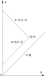
Expressions in the left-hand side of (19) are the total derivatives of $\psi_{1}$ and $\psi_{2}$ along corresponding characteristics (see Fig.1). Integrating the first equation along the lower characteristics, and the second equation - along the upper one, we obtain for $t>y$

(21) $$\left\{\begin{array}[]{rcl}\psi_{1}(y,t)&=&\int\limits_{0}^{y}\psi_{2}(\eta,t+\eta-y)d\eta,\\ \psi_{2}(y,t)&=&-\int\limits_{0}^{y}q(\eta,\xi)\psi_{1}(\eta,t-\eta+y)d\eta+g(t+y,\xi),\end{array}\right.$$

where

(22) $$g(t,\xi)=\delta^{\prime}(t)+\frac{n_{0}^{\prime}(0)}{2n_{0}(0)}\delta(t)+\frac{r_{0}(t,\xi)}{\sqrt{\rho_{1}n_{0}(0)}}$$

is bounded as $t\to 0$ due to the cancellation of $\delta^{\prime}(t)-$ and $\delta(t)-$ singularities in the right-hand side of (22).

Figure 1. Integration along characteristic lines: integral for $\psi_{1}$ is along $\tau=\eta+t-y$, for $\psi_{2},\,q$ - along $\tau=t+y-\eta$

The system (21) is not complete to solve the inverse problem as it has three unknown functions $\psi_{1}(y,t)$, $\psi_{2}(y,t)$ and $q(y,\xi)$ and just two equations. We use the progressive wave expansion, see e.g. [6], [30],

(23) $$U^{(0)}(y,t)=\sum_{n=0}f_{n}(t-y)U^{(0)}_{n}(y),\quad f_{n+1}(t)=\int\limits_{0}^{t}f_{n}(t)dt,\quad f_{0}(t)=\delta(t)$$

to derive the third equation. The amplitudes $U^{(0)}_{n}$ are found from the transport equations with e.g.

(24) $$U^{(0)}_{0}=\frac{1}{\sqrt{\sigma(y)}},\quad U^{(0)}_{1}=\frac{1}{2\sqrt{\sigma(y)}}\int\limits_{0}^{y}q(\eta)d\eta,$$

so that

$$\psi_{2}(y,t)=\frac{1}{2}\theta(t-y)q(y)+....$$

Here and later we often skip the dependence of $q$ and other functions on $\xi$ when our considerations are independent of its value.

Substituting the second equation of (21) into this relation, and taking $t\to y+0$, we obtain the third desired equation. We summarize the above results in the follwing

Proposition 3.1.

Let $\psi_{1,2}(y,t)$ is obtained from the solution $U^{(0)}(y,t)$ of the wave equation (17) by formula (18). Then $\psi_{1,2}(y,t)$ together with $q(y)$ satisfy the following system of non-linear Volterra-type equations,

(25) $$\left\{\begin{array}[]{rcl}\psi_{1}(y,t)&=&\int\limits_{0}^{y}\psi_{2}(\eta,t+\eta-y)d\eta,\\ \psi_{2}(y,t)&=&-\int\limits_{0}^{y}q(\eta)\psi_{1}(\eta,t-\eta+y)d\eta+g(t+y),\\ q(y)&=&-2\int\limits_{0}^{y}q(\eta)\psi_{1}(\eta,2y-\eta)d\eta+2g(2y).\end{array}\right.$$

This non-linear Volterra-type system of integral equations, in the sense of Goh’berg-Krein [18], allows us to determine, at least locally, the function $q(y)$ from the response $g(t)$ for $0<t<2T$. In section 5 we return to the question of the global solvability of system (25). Having solved this system for two different values $\xi_{1}$ and $\xi_{2}$, we determine the refractive index in the zero-approximation,

(26) $$n_{0}(y)=\sqrt{\frac{|\xi|_{2}^{2}-|\xi|_{1}^{2}}{q(y,\xi_{1})-q(y,\xi_{2})}},$$

which must be used together with

$$z=\int\limits_{0}^{y}\frac{dy}{n_{0}(y)}.$$

The refractive index $n_{0}(y)$ may also be determined by solving system (25) just for a single value of $\xi$. It can be done by integration the differential equation for $w(y)=\sqrt{\sigma(y)}$ which follows from (20)

$$w^{\prime\prime}+wq(y,\xi)=-\frac{|\xi|^{2}}{\rho_{1}^{2}w^{3}}.$$

The general solution of this equation may be represented in the form, see [1].

$$w(y)=\sqrt{\sum_{i,j=1,2}A_{i,j}w_{i}(y)w_{j}(y)},$$

where $w_{1,2}(y)$ make a fundamental system of the corresponding homogeneous equation. Constant real symmetric matrix $A_{i,j}$ satisfies

$${\rm det}||A_{i,j}||W^{2}(w_{1},w_{2})=-\frac{|\xi|^{2}}{\rho^{2}_{1}},$$

where

$$W(w_{1},w_{2})=w_{1}w_{2}^{\prime}-w_{1}^{\prime}w_{2}.$$

Given $w(0)$ and $w^{\prime}(0)$ we are then able to determine all entries of the matrix $A$.

3.2. Two layers problem

Consider a wave propagation through the interface, $y=y(h_{0})=L$, using the singularity analysis of the incident, reflected and transmitted waves. Then, in the layer $0<y<L$, the singularities of $U^{(0)}$ given by the incident and reflected waves, are

$$U^{(0)}=\frac{\delta(t-y)}{\sqrt{\sigma(y)}}+d_{0}\frac{\delta(t+y-2L)}{\sqrt{\sigma(y)}}+$$

$$+\frac{\theta(t-y)}{2\sqrt{\sigma(y)}}Q_{0}(y)+\frac{\theta(t+y-2L)}{2\sqrt{\sigma(y)}}(d_{1}+Q_{1}(y))+...,\quad 0<y<L,\,\,L<t<2L.$$

For the transmitted wave, the WKB asymptotics is given by

$$U^{(0)}=s_{0}\frac{\delta(t-y)}{\sqrt{\sigma(y)}}+\frac{\theta(t-y)}{2\sqrt{\sigma(y)}}(s_{1}+Q_{1}(y))+...,\quad y>L,\,\,L<t<2L,$$

where

$$Q_{0}(y)=\int\limits_{0}^{y}q(\eta)d\eta,\quad Q_{1}(y)=\int\limits_{L}^{y}q(\eta)d\eta.$$

Unknown quatities $d_{0}$, $d_{1}$ and $s_{0}$, $s_{1}$ are the reflection and transmission coefficients. Using the interface continuity conditions (11), leads to a linear system of equations for $d_{0}$, $d_{1}$ and $s_{0}$, $s_{1}$ so that

(27) $$d_{0}=\frac{1-\frac{\sigma_{+}}{\sigma_{-}}}{1+\frac{\sigma_{+}}{\sigma_{-}}},\quad d_{1}=\frac{\sigma^{\prime}_{-}(1+d_{0})+Q_{0}(L)(\sigma_{-}-\sigma_{+})-s_{0}\sigma^{\prime}_{+}\sqrt{\frac{\sigma_{-}}{\sigma_{+}}}}{\sigma_{+}+\sigma_{-}},$$

$$s_{0}=\sqrt{\frac{\sigma_{+}}{\sigma_{-}}}\frac{2}{1+\frac{\sigma_{+}}{\sigma_{-}}},\quad s_{1}=\sqrt{\frac{\sigma_{+}}{\sigma_{-}}}\frac{\sigma^{\prime}_{-}(1+d_{0})+2Q_{0}(L)\sigma_{-}-s_{0}\sigma^{\prime}_{+}\sqrt{\frac{\sigma_{-}}{\sigma_{+}}}}{\sigma_{+}+\sigma_{-}},$$

where $\sigma_{\pm}$ and $\sigma^{\prime}_{\pm}$ are the limiting values of $\sigma(y)$ and $\sigma^{\prime}(y)$ at $y\to L-0$ and $y\to L+0$, correspondingly.

Figure 2. Characteristic lines in the case of two layers.

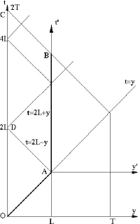
Analyzing the incoming singularities at $y=0$, we can find $L$ and, therefore, $h-0$ and also $d_{0}$ and $d_{1}$. This will give us $\sigma_{+}$ and $\sigma^{\prime}_{+}$. The next step is reconstruction of the velocity at large depth $L<y<T$, which is illustrated on Fig. 2. This reconstruction requires the data observed for $0<t<2T$. At this stage we again apply the non-linear Volterra system of integral equations (25) in the new frame $y^{\prime},\eta^{\prime},t^{\prime}$ ($y=y^{\prime}+L,\,\eta=\eta^{\prime}+L,\,t=t^{\prime}+L$)

(28) $$\left\{\begin{array}[]{rcl}\psi_{1}(y^{\prime},t^{\prime})&=&\int\limits_{0}^{y^{\prime}}\psi_{2}(\eta^{\prime},t^{\prime}+\eta^{\prime}-y^{\prime})d\eta^{\prime}+\psi_{1}^{+}(0,t^{\prime}-y^{\prime}),\\ \psi_{2}(y^{\prime},t^{\prime})&=&-\int\limits_{0}^{y^{\prime}}q(\eta^{\prime})\psi_{1}(\eta^{\prime},t^{\prime}-\eta^{\prime}+y^{\prime})d\eta^{\prime}+\psi_{2}^{+}(0,t^{\prime}+y^{\prime}),\\ q(y^{\prime})&=&-2\int\limits_{0}^{y^{\prime}}q(\eta^{\prime})\psi_{1}(\eta^{\prime},2y^{\prime}-\eta^{\prime})d\eta^{\prime}+2\psi_{2}^{+}(0,2y^{\prime}).\end{array}\right.$$

These require knowledge of $\psi_{1}^{+}(0,t^{\prime}-y^{\prime})$ and $\psi_{2}^{+}(0,t^{\prime}+y^{\prime})$ at the vertical segment $AB$ as the limits $\psi_{1,2}^{+}(0,t)=\lim\psi_{1,2}(y,t)$ for $y\to L+0$. To this end, we first determine $\psi^{-}_{1,2}(0,t)=\lim\psi_{1,2}(y,t)$ for $y\to L-0$ using system (21). Employing the interface continuity conditions

$$\frac{\psi^{-}_{1}}{\sqrt{\sigma_{-}}}=\frac{\psi^{+}_{1}}{\sqrt{\sigma_{+}}},\quad\psi^{-}_{1y}\sqrt{\sigma_{-}}-\psi^{-}_{1}\frac{\sigma^{\prime}_{-}}{2\sqrt{\sigma_{-}}}=\psi^{+}_{1y}\sqrt{\sigma_{+}}-\psi^{+}_{1}\frac{\sigma^{\prime}_{+}}{2\sqrt{\sigma_{+}}},$$

we obtain the required data, $\psi_{1}^{+}(0,t^{\prime}-y^{\prime})$ and $\psi_{2}^{+}(0,t^{\prime}+y^{\prime})$ at $AB$.

4. Inverse problem in the first-order approximation

4.1. Half-space

In this section we describe an algorithm to determine $\bar{n}(z)$ in an inhomogeneous half-space from the response $r_{1}(t,\xi)$. For convenience, we integrate all the functions of the zero-order problem with respect to time $t$ so that

$$U^{(0)}\bigg{|}_{y=0}=\theta(t)\sqrt{\frac{\rho_{1}}{n_{0}(0)}}.$$

Using the variables $y$ and $\sigma(y)$, we rewrite the problem (13), (14) in the form

(29) $$U^{(1)}_{tt}-\frac{1}{\sigma(y)}\frac{\partial}{\partial y}\bigg{(}\sigma(y)U^{(1)}_{y}\bigg{)}+\frac{|\xi|^{2}}{n_{0}^{2}}U^{(1)}=\frac{1}{n_{0}^{2}}<\bar{n},\nabla_{\xi}U^{(0)}_{tt}>,$$

$$U^{(1)}\bigg{|}_{y=0}=0,\quad U^{(1)}_{y}\bigg{|}_{y=0}=\frac{\hat{r}_{1}(t,\xi)}{n_{0}(0)},\quad\hat{r}_{1}(t,\xi)=\int\limits_{0}^{t}r_{1}(t,\xi)dt.$$

We start with the progressive wave expansion for $U^{(1)}$. As by (23), (24),

$$<\bar{n},\nabla_{\xi}U^{(0)}_{tt}>=-<\bar{n},\xi>\frac{\delta(t-y)}{\sqrt{\sigma(y)}}\int\limits_{0}^{y}\frac{d\eta}{n_{0}^{2}(\eta)}+...~{}~{}.$$

the progressive wave expansion for $U^{(1)}(y,t)$ has the form

$$U^{(1)}(y,t)=\theta(t-y)A_{0}(y)+(t-y)_{+}A_{1}(y)+....$$

Therefore, equation (29) implies, in particular, that

(30) $$A_{0}(y)=\frac{1}{\sqrt{\sigma(y)}}\int\limits_{0}^{y}<\bar{n}(\eta),\xi>p(\eta)d\eta,\quad p(y)=-\frac{1}{2n_{0}^{2}(y)}\int\limits_{0}^{y}\frac{d\eta}{n_{0}^{2}(\eta)}.$$

Let $G(y,\eta,t;\xi)$ be the space-causal Green’s function,

(31) $$G_{tt}-\frac{1}{\sigma(y)}\frac{\partial}{\partial y}\bigg{(}\sigma(y)G_{y}\bigg{)}+\frac{|\xi|^{2}}{n_{0}^{2}}G=\delta(t)\delta(y-\eta),\quad G=0\,\,{\rm if}\,\,y<\eta.$$

Then

(32) $$U^{(1)}(y,y+0;\xi)=$$

$$\int\limits_{0}^{y}d\eta\int\limits_{\eta}^{2y-\eta}d\tau G(y,\eta,y-\tau;\xi)\frac{<\bar{n},\nabla_{\xi}U^{(0)}_{tt}(\eta,\tau;\xi)>}{n_{0}^{2}(\eta)}-\frac{1}{n_{0}(0)}\int\limits_{0}^{2y}d\tau G(y,0,y-\tau;\xi)\hat{r}_{1}(\tau,\xi),$$

where we now write down explicitly the dependence on $\xi$.

Introducing new unknown functions,

(33) $$\bar{\varphi}(y)=(\varphi_{1}(y),\varphi_{2}(y))=\bar{n}(y)p(y)$$

and employing the progressive wave expansion for $U^{(1)}$, we see that

$$<\bar{\varphi}(y),\xi>=\frac{d}{dy}\Bigg{\{}\sqrt{\sigma(y)}\int\limits_{0}^{y}d\eta\int\limits_{\eta}^{2y-\eta}d\tau G(y,\eta,y-\tau,\xi)\frac{<\bar{\varphi}(\eta),\nabla_{\xi}U^{(0)}_{tt}(\eta,\tau,\xi)>}{n_{0}^{2}(\eta)p(\eta)}$$

(34) $$-\frac{\sqrt{\sigma(y)}}{n_{0}(0)}\int\limits_{0}^{2y}d\tau G(y,0,y-\tau,\xi)\hat{r}_{1}(\tau,\xi)\Bigg{\}}.$$

Finally, the desired system of linear Volterra integral equations may be obtained from (34) by differentiation and setting $\xi$ equal to e.g. $\xi_{1}=(a,0)$ and $\xi_{2}=(0,a)$, where $a\neq 0$. Namely, we obtain

Proposition 4.1.

Let $\bar{\varphi}(y)=(\varphi_{1}(y),\varphi_{2}(y))$ be given by (33) where the scalar factor $p(y)$ depends only on the already found $n_{0}(y)$. Then $\bar{\varphi}(y)$ satisfies the system of linear Volterra equations

$$a\varphi_{i}(y)=2\int\limits_{0}^{y}d\eta G_{1}(y,\eta,\eta-y,\xi_{i})\frac{<\bar{\varphi}(\eta),\nabla_{\xi}U^{(0)}_{tt}(\eta,2y-\eta,\xi_{i})>}{n_{0}^{2}(\eta)p(\eta)}$$

$$-\frac{2}{n_{0}(0)}G_{1}(y,0,-y,\xi_{i})\hat{r}_{1}(2y,\xi_{i})+\int\limits_{0}^{y}d\eta\int\limits_{\eta}^{2y-\eta}d\tau G_{2}(y,\eta,y-\tau,\xi_{i})\frac{<\bar{\varphi}(\eta),\nabla_{\xi}U^{(0)}_{tt}(\eta,\tau,\xi_{i})>}{n_{0}^{2}(\eta)p(\eta)}-$$

$$-\frac{1}{n_{0}(0)}\int\limits_{0}^{2y}d\tau G_{2}(y,0,y-\tau,\xi_{i})\hat{r}_{1}(\tau,\xi_{i}),\quad i=1,2.$$

where

$$G_{1}(y,\eta,t-\tau;\xi)=\sqrt{\sigma(y)}G(y,\eta,t-\tau;\xi)\quad G_{2}(y,\eta,t-\tau;\xi)=G_{1t}(y,\eta,t-\tau;\xi)+G_{1y}(y,\eta,t-\tau;\xi).$$

Observe that, due to the first equation in (25),

$$\lim_{\eta\to 0}\nabla_{\xi}U^{(0)}_{tt}(\eta,\tau)=0,$$

so that the system of integral equtions in Proposition 4.1 is not singular.

4.2. Two layers problem

Let us consider the inverse problem for the first-order approximation in the case of a layer and a semi-infinite bottom separated by an interface. Our goal is to derive a coupled system of linear Volterra integral equations similar to that in Proposition 4.1 to reconstruct $\bar{n}(z)$ and also to determine constants $\bar{h}$ characterizing this interface. Recall the formulation of the corresponding problem using $y$ variable, see (13), (14),

(35) $$U^{(1)}_{tt}-\frac{1}{\sigma(y)}\frac{\partial}{\partial y}\bigg{(}\sigma(y)U^{(1)}_{y}\bigg{)}+\frac{\xi^{2}}{n_{0}^{2}}U^{(1)}=\frac{1}{n_{0}^{2}}<\bar{n},\nabla_{\xi}U^{(0)}_{tt}>,$$

$$U^{(1)}\bigg{|}_{y=0}=0,\quad U^{(1)}_{y}\bigg{|}_{y=0}=\frac{\hat{r}_{1}(t,\xi)}{n_{0}(0)}.$$

$$\bigg{[}U^{(1)}-n_{0}<\bar{h},\nabla_{\xi}U^{(0)}_{y}>\bigg{]}\bigg{|}_{y=L}=0,$$

$$\bigg{[}\sigma(y)U^{(1)}_{y}-\bigg{(}\rho\sigma^{2}(y)<\bar{h},\nabla_{\xi}U^{(0)}_{yy}>+\rho\sigma(y)\sigma^{\prime}(y)<\bar{h},\nabla_{\xi}U^{(0)}_{y}>-U^{(0)}\frac{<\xi,\bar{h}>}{\rho}\bigg{)}\bigg{]}\bigg{|}_{y=L}=0.$$

As before, we start with the singularity analysis of the transmitted and reflected waves. The progressive wave expansion of the inhomogeneous term in (35) is given by

$$\frac{\partial}{\partial\xi_{i}}U^{(0)}_{tt}=-\frac{\xi_{i}\delta(t-y)}{\sqrt{\sigma(y)}}\int\limits_{0}^{y}\frac{d\eta}{n_{0}^{2}(\eta)}+\frac{\delta(t+y-2L)}{\sqrt{\sigma(y)}}\bigg{(}\frac{1}{2}\frac{\partial}{\partial\xi_{i}}d_{1}-\xi_{i}\int\limits_{L}^{y}\frac{d\eta}{n_{0}^{2}(\eta)}\bigg{)}+...~{}~{},$$

$$0<y<L,\,\,L<t<2L,\,\,i=1,2,$$

$$\frac{\partial}{\partial\xi_{i}}U^{(0)}_{tt}=\frac{\delta(t-y)}{\sqrt{\sigma(y)}}\bigg{(}\frac{1}{2}\frac{\partial}{\partial\xi_{i}}s_{1}-\xi_{i}\int\limits_{L}^{y}\frac{d\eta}{n_{0}^{2}(\eta)}\bigg{)}+...~{}~{},\quad y>L,\,\,L<t<3L.$$

Then the sum of the incident and reflected waves is given by

(36) $$U^{(1)}=\frac{\theta(t-y)}{\sqrt{\sigma(y)}}\int\limits_{0}^{y}<\bar{n},\xi>p(\eta)d\eta+\frac{\theta(t+y-2L)}{\sqrt{\sigma(y)}}\bigg{(}\int\limits_{L}^{y}<\bar{n},\bar{p}_{1}>d\eta+D\bigg{)}+...~{}~{},$$

$$0<y<L,\,\,L<t<2L,$$

where

$$\bar{p}_{1}^{(i)}(y)=\frac{1}{2n_{0}^{2}(y)}\bigg{(}\frac{1}{2}\frac{\partial}{\partial\xi_{i}}d_{1}-\xi_{i}\int\limits_{L}^{y}\frac{d\eta}{n_{0}^{2}(\eta)}\bigg{)},~{}~{}~{}~{}~{}0<y<L.$$

The transmitted wave is then

(37) $$U^{(1)}=\frac{\theta(t-y)}{\sqrt{\sigma(y)}}\bigg{(}\int\limits_{L}^{y}<\bar{n},\bar{p}_{2}>d\eta+S\bigg{)}+...,\quad y>L,\,\,L<t<3L,$$

where

$$\bar{p}_{2}(y)=\frac{1}{2n_{0}^{2}(y)}\bigg{(}\frac{1}{2}\frac{\partial}{\partial\xi_{i}}s_{1}-\xi\int\limits_{L}^{y}\frac{d\eta}{n_{0}^{2}(\eta)}\bigg{)},\quad y>L$$

and coefficients $d_{1},s_{1}$ are defined in (27).

Substituting these expressions for $U^{(1)}$ into the interface continuity relations in (35), and solving the corresponding system of linear equations, we find that

(38) $$D(\xi)=\frac{\bigg{(}1-\frac{\sigma_{+}}{\sigma_{-}}\bigg{)}\int\limits_{0}^{L}<\bar{n},\xi>p(y)dy+\frac{\sigma_{+}}{\sigma_{-}}<\bar{h},\bar{\Gamma}_{1}>+<\bar{h},\bar{\Gamma}_{2}>}{1+\frac{\sigma_{+}}{\sigma_{-}}},$$

$$S(\xi)=\frac{2\int\limits_{0}^{L}<\bar{n},\xi>p(y)dy+<\bar{h},\bar{\Gamma}_{2}-\bar{\Gamma}_{1}>}{\sqrt{\frac{\sigma_{-}}{\sigma_{+}}}+\sqrt{\frac{\sigma_{+}}{\sigma_{-}}}}.$$

Here the vectors $\bar{\Gamma}_{1}$ and $\bar{\Gamma}_{2}$ are given by

$$\bar{\Gamma}_{1}^{(i)}=\rho_{1}\sigma_{-}\bigg{(}\frac{\partial}{2\partial\xi_{i}}d_{1}+\xi_{i}\int\limits_{0}^{L}\frac{d\eta}{n_{0}^{2}(\eta)}\bigg{)}+\sqrt{\frac{\sigma_{-}}{\sigma_{+}}}\rho_{2}\sigma_{+}\frac{1}{2}\frac{\partial}{\partial\xi_{i}}s_{1},$$

$$\bar{\Gamma}_{2}^{(i)}=\rho_{1}\sigma_{-}\bigg{(}\frac{\partial}{2\partial\xi_{i}}d_{1}-\xi_{i}\int\limits_{0}^{L}\frac{d\eta}{n_{0}^{2}(\eta)}\bigg{)}-\sqrt{\frac{\sigma_{+}}{\sigma_{-}}}\rho_{2}\sigma_{+}\frac{1}{2}\frac{\partial}{\partial\xi_{i}}s_{1},\quad i=1,2.$$

From the jump of $U^{(1)}$ at $y=0$ at the time $t=2L$, we can find $D$. Now equation (38) with $\xi_{1}=(a,0)$ and $\xi_{2}=(0,a)$ make possible to find $\bar{h}$,

(39) $$h_{i}=\bigg{[}D(\xi_{i})\bigg{(}1+\frac{\sigma_{+}}{\sigma_{-}}\bigg{)}-\bigg{(}1-\frac{\sigma_{+}}{\sigma_{-}}\bigg{)}\int\limits_{0}^{L}<\bar{n},\xi_{i}>p(y)dy\bigg{]}\bigg{[}2a\rho_{1}\frac{\sigma_{+}-\sigma_{-}}{\sigma_{+}+\sigma_{-}}\int\limits_{0}^{L}\frac{d\eta}{n_{0}^{2}(\eta)}\bigg{]}^{-1}.$$

Clearly, at this stage we can also find $S$.

Let us describe an algorithm to determine $\bar{n}(z)$ in the second layer. The boundary conditions $U^{(1)}|_{y=L+0}$ and the response $U^{(1)}_{y}|_{y=L+0}$ for the transmitted wave can be found using $\hat{r}_{1}(t,\xi)$ and already known, in the upper layer, $n_{0}(y),\,\bar{n}(y)$ together with the interface continuity conditions in (35). Using the coordinates $y^{\prime},\eta^{\prime},t^{\prime},\,y=y^{\prime}+L,\eta=\eta^{\prime}+L,\,\,t=t^{\prime}+L$, see Fig. 1, we have the progressive wave expansion for $U^{(1)}$,

$$U^{(1)}(y^{\prime},t^{\prime})=\frac{\theta(t-y^{\prime})}{\sqrt{\sigma(y^{\prime})}}\bigg{(}\int\limits_{0}^{y^{\prime}}<\bar{n},\xi>p_{2}(\eta)d\eta+S\bigg{)}+...,\quad\bar{p}_{2}(y^{\prime})=\xi p_{2}(y^{\prime}).$$

Employing the Green function (31) in the second layer, we obtain

$$p_{2}(y^{\prime})<\bar{n}(y^{\prime}),\xi>=$$

$$\frac{d}{dy^{\prime}}\Bigg{\{}\sqrt{\sigma(y^{\prime})}\bigg{(}\int\limits_{0}^{y^{\prime}}d\eta^{\prime}\int\limits_{\eta^{\prime}}^{2y^{\prime}-\eta^{\prime}}d\tau G(y^{\prime},\eta^{\prime},y^{\prime}-\tau)\frac{<\bar{n}(\eta^{\prime}),\nabla_{\xi}U^{(0)}_{tt}(\eta^{\prime},\tau,\xi)>}{n_{0}^{2}(\eta^{\prime})}$$

$$-\int\limits_{0}^{2y^{\prime}}d\tau G(y^{\prime},0,y^{\prime}-\tau)\left(\chi_{2}(\tau)+\frac{\sigma^{\prime}_{+}}{\sigma_{+}}\chi_{1}(\tau)\right)+\int\limits_{0}^{2y^{\prime}}d\tau G_{\eta^{\prime}}(y^{\prime},0,y^{\prime}-\tau)\chi_{1}(\tau)$$

$$+[G(y^{\prime},0,y^{\prime})\chi_{1}(0)-G(y^{\prime},0,-y^{\prime})\chi_{1}(2y^{\prime})]\bigg{)}\Bigg{\}},$$

where

$$\chi_{1}(t)=U^{(1)}|_{y=L},\quad\chi_{2}(t)=U^{(1)}_{y}|_{y=L}$$

Finally, the desired coupled system of linear Volterra integral equations determining $\bar{n}(y)$ below the interface may be obtained from this equation by setting e.g. $\xi_{1}=(a,0)$ and $\xi_{2}=(0,a)$ (compare with Proposition 4.1). It is worth noting that these integral equations are not singular.

5. Global reconstruction and stability

As mentioned in section 3, the non-linear Volterra-type system of integral equations (25) may, in principle, be solvable only locally. In this section we show that, assuming a priori bounds for $q(t)$ in $C(0,T)$, it can be found on the whole interval $(0,T)$ using a layer-stripping method based on (25). What is more, we will prove Lipschitz stability of this procedure with respect to the variation of the response data $g(t)$ in $C(0,2T)$.

We first note that if $||q||_{C(0,T)}<M$ then solving the direct problem gives

(40) $$||\psi_{1,2}||_{C(\Delta_{T})},\,\,||q||_{C(0,T)}<A=A(T,M),$$

where we can assume $A\geq\max(1,M)$. Here $\Delta_{T}$ and generally $\Delta_{b},\,0<b<T$, is the triangle in $R^{2}$ bounded by the characteristics $\eta=\tau,\,\eta+\tau=2b$ and the axis $\eta=0$. Assume that we have already found $\psi_{1,2}$ in $\Delta_{b}$ and $q$ in $(0,b)$.

Lemma 5.1.

Let $\lambda>0$ satisfies

(41) $$\lambda<\frac{1}{16(1+A)^{2}}.$$

Then system (25) uniquely determines $\psi_{1,2}(y,t),\,q(y)$ for $(y,t)\in\Delta_{b+\lambda}$, $y\in(0,b+\lambda)$, respectively. Moreover, these functions can be found from system (25) by Picard iterations.

Proof Utilizing new coordinates $y^{\prime}=y-b,\,\eta^{\prime}=\eta-b,\,t^{\prime}=t-b$ (compare with the end of section 3), we obtain a system of non-linear Volterra-type equations similar to (28),

(42) $$\left\{\begin{array}[]{rcl}\psi_{1}(y^{\prime},t^{\prime})&=&\int\limits_{0}^{y^{\prime}}\psi_{2}(\eta^{\prime},t^{\prime}+\eta^{\prime}-y^{\prime})d\eta^{\prime}+g_{1}(y^{\prime},t^{\prime}),\\ \psi_{2}(y^{\prime},t^{\prime})&=&-\int\limits_{0}^{y^{\prime}}q(\eta^{\prime},\xi)\psi_{1}(\eta^{\prime},t^{\prime}-\eta^{\prime}+y^{\prime})d\eta^{\prime}+g_{2}(y^{\prime},t^{\prime}),\\ q(y^{\prime})&=&-2\int\limits_{0}^{y^{\prime}}q(\eta^{\prime})\psi_{1}(\eta^{\prime},2y^{\prime}-\eta^{\prime})d\eta^{\prime}+g_{3}(y^{\prime}).\end{array}\right.$$

Here $g_{1}(y^{\prime},t^{\prime})=\psi_{1}(0,t^{\prime}-y^{\prime}),\quad g_{2}(y^{\prime},t^{\prime})=\psi_{2}(0,t^{\prime}=y^{\prime}),\quad g_{3}(y^{\prime})=2\psi_{2}(0,2y^{\prime})$ may be found from the "direct" system (21) and satisfy $|g_{i}|<A$.

Using the first equation in (42), we eliminate $\psi_{1}$ to get

(43) $$\left\{\begin{array}[]{rcl}\psi_{2}(y^{\prime},t^{\prime})&=&-\int\limits_{0}^{y^{\prime}}q(\eta^{\prime},\xi)\left[g_{1}(\eta^{\prime},t^{\prime}-\eta^{\prime}+y^{\prime})+\int_{0}^{\eta^{\prime}}\psi_{2}(\xi^{\prime},t^{\prime}-\eta^{\prime}+\xi^{\prime})d\xi^{\prime}\right]d\eta^{\prime}+g_{2}(y^{\prime},t^{\prime}),\\ q(y^{\prime})&=&-2\int\limits_{0}^{y^{\prime}}q(\eta^{\prime})\left[g_{1}(\eta^{\prime},2y^{\prime}-\eta^{\prime})+\int_{0}^{\eta^{\prime}}\psi_{2}(\xi^{\prime},y^{\prime}-\eta^{\prime}+\xi^{\prime})d\xi^{\prime}\right]d\eta^{\prime}+g_{3}(y^{\prime}).\end{array}\right.$$

We rewrite this system in the form,

$$(\psi_{2},\,q)=K_{\lambda}(\psi_{2},\,q),$$

where $K_{\lambda}$ is a non-linear operator in $C(\Delta_{\lambda}\times C(0,\lambda)$ determined by the right-hand side (43). Let us show that $K_{\lambda}$ is a contraction in

$${\bf D}_{2A}=B_{2A}(C(\Delta_{\lambda}))\times B_{2A}(C(0,\lambda)),$$

where $B_{\rho}(\cdot)$ is the ball of radius $\rho$ in the corresponding function space and we use the norm

$$||(\psi_{2},\,q)||=\max(||\psi_{2}||,\,||q||).$$

Considering

$$K_{\lambda}(\psi_{2},q)-K_{\lambda}({\hat{\psi}}_{2},{\hat{q}})=\left(K_{\lambda}(\psi_{2},q)-K_{\lambda}(\psi_{2},{\hat{q}})\right)+\left(K_{\lambda}(\psi_{2},{\hat{q}})-K_{\lambda}({\hat{\psi}}_{2},{\hat{q}})\right),$$

it follows from (43) that in ${\bf D}_{2A}$

$$||K_{\lambda}(\psi_{2},q)-K_{\lambda}({\hat{\psi}}_{2},{\hat{q}})||\leq 2A\lambda\left(||q-{\hat{q}}||+2\lambda||\psi_{2}-{\hat{\psi}}_{2}||+2\lambda||q-{\hat{q}}||\right).$$

As $\lambda$ satisfies (41), this implies that

$$||K_{\lambda}(\psi_{2},q)-K_{\lambda}({\hat{\psi}}_{2},{\hat{q}})||\leq\frac{3}{8}||(\psi_{2},\,q)-({\hat{\psi}}_{2},{\hat{q}})||.$$

Similar arguments show that $K_{\lambda}:{\bf D}_{2A}\rightarrow{\bf D}_{2A}$. Thus (43) has a unique solution in ${\bf D}_{2A}$ and, since (28) is a Volterra-type system, in $C(\Delta_{\lambda})\times C(0,\lambda)$.

QED

Next we prove the Lipschitz stability of the non-linear Volterra system (25). Let us denote by $\tilde{\psi}_{1,2}(y,t)$, $\tilde{q}(y,\xi)$ and $\tilde{g}(t)$ small variations of the corresponding functions.

Lemma 5.2.

Let $\psi_{1,2},\,q$ satisfy (40). There exist $c_{0}=c_{0}(T,A),\,\epsilon_{0}=\epsilon-0(T,A)$ such that for $||\tilde{g}||_{C(0,2T)}<\epsilon<\epsilon_{0}$ the corresponding system (25) with $g+\tilde{g}$ instead of $g$ has a unique solution $\psi_{1,2}+\tilde{\psi}_{1,2}$, $q+\tilde{q}$, and

(44) $$||\tilde{\psi}_{1,2}||_{C(\Delta_{T})},\,\,||\tilde{q}||_{C(0,2T)}<c_{0}\epsilon.$$

Proof Substituting expressions for $\psi_{1,2}(y,t)+\tilde{\psi}_{1,2}(y,t)$, $q(y)+\tilde{q}(y)$ and $g(t)+\tilde{g}(t)$ into (25) , we obtain the corresponding system in variations

$$\left\{\begin{array}[]{rcl}\tilde{\psi}_{1}(y,t)&=&\int\limits_{0}^{y}\tilde{\psi}_{2}(\eta,t+\eta-y)d\eta,\\ \tilde{\psi}_{2}(y,t)&=&-\int\limits_{0}^{y}q(\eta)\tilde{\psi}_{1}(\eta,t-\eta+y)d\eta\\ &&-\int\limits_{0}^{y}\tilde{q}(\eta)(\psi_{1}(\eta,t-\eta+y)+\tilde{\psi}_{1}(\eta,t-\eta+y))d\eta+\tilde{g}(t+y),\\ \tilde{q}(y)&=&-2\int\limits_{0}^{y}\tilde{q}(\eta)\psi_{1}(\eta,2y-\eta)d\eta-2\int\limits_{0}^{y}(q(\eta)+\tilde{q}(\eta))\tilde{\psi}_{1}(\eta,2y-\eta)d\eta+2\tilde{g}(2y).\end{array}\right.$$

Let $||\tilde{g}||<\epsilon$. Then, we have

$$\left\{\begin{array}[]{rcl}|\tilde{\psi}_{1}(y,t)|&\leq&\int\limits_{0}^{y}|\tilde{\psi}_{2}(\eta,t+\eta-y)|d\eta,\\ |\tilde{\psi}_{2}(y,t)|&\leq&2A\int\limits_{0}^{y}|\tilde{\psi}_{1}(\eta,t-\eta+y)|d\eta+A\int\limits_{0}^{y}|\tilde{q}(\eta)|d\eta+\epsilon,\\ |\tilde{q}(y)|&\leq&4A\int\limits_{0}^{y}|\tilde{q}(\eta)|d\eta+2A\int\limits_{0}^{y}|\tilde{\psi}_{1}(\eta,2y-\eta)|d\eta+2\epsilon.\end{array}\right.$$

Substituting the upper inequality into the second one to replace $|\tilde{\psi}_{1}(\eta,t-\eta+y)|$, we obtain

$$|\tilde{\psi}_{2}(y,t)|\leq 2A\int\limits_{\Delta_{y,t}}|\tilde{\psi}_{2}(\eta,\tau)|d\eta d\tau+2A\int\limits_{0}^{y}|\tilde{q}(\eta)|d\eta+\epsilon,$$

where $\Delta_{y,t}$ is the the triangle in $R^{2}$ bounded by the characteristics $\tau=\eta+t-y,\,\tau=t+y-\eta$ and the axis $\eta=0$. Similarly,

$$|\tilde{q}(y)|\leq 4A\int\limits_{0}^{y}|\tilde{q}(\eta)|d\eta+4A\int\limits_{\Delta_{y,t}}|\tilde{\psi}_{2}(\eta,\tau)|d\eta d\tau+2\epsilon.$$

Let

$$p(\eta)={\rm max}_{\tau}|\tilde{\psi}_{2}(\eta,\tau)|,\quad(\eta,\tau)\in\Delta_{T}.$$

Then, we have

$$|\tilde{\psi}_{2}(y,t)|\leq 4AT\int\limits_{0}^{y}p(\eta)d\eta+2A\int\limits_{0}^{y}|\tilde{q}(\eta)|d\eta+\epsilon,$$

$$|\tilde{q}(y)|\leq 4A\int\limits_{0}^{y}|\tilde{q}(\eta,\xi)|d\eta+8AT\int\limits_{0}^{y}p(\eta)d\eta+2\epsilon,$$

as

$$\int\limits_{\Delta_{y,t}}p(\eta)d\eta d\tau=2\int\limits_{0}^{y}p(\eta)(y-\eta)d\eta\leq 2T\int\limits_{0}^{y}p(\eta)d\eta.$$

Moreover, it holds that

$$p(y)\leq 4AT\int\limits_{0}^{y}p(\eta)d\eta+2A\int\limits_{0}^{y}|\tilde{q}(\eta)|d\eta+\epsilon.$$

Introduce

$$\rho(y)=p(y)+|\tilde{q}(y)|.$$

Adding the last two inequalities for $p(y)$ and $|\tilde{q}(y)|$ yields

$$\rho(y)\leq\int\limits_{0}^{y}(12ATp(\eta)+6A|\tilde{q}(\eta)|)d\eta+3\epsilon,$$

or, with $C=6A{\rm max}(1,2T)$,

$$\rho(y)\leq C\int\limits_{0}^{y}\rho(\eta)d\eta+3\epsilon\leq C\int\limits_{0}^{y}\bigg{(}C\int\limits_{0}^{\eta}\rho(\eta_{1})d\eta_{1}+3\epsilon\bigg{)}d\eta+3\epsilon=$$

$$\frac{C^{2}}{1!}\int\limits_{0}^{y}\rho(\eta)(y-\eta)d\eta+(Cy+1)3\epsilon.$$

Continuing this process, we come to the estimate

$$\rho(y)\leq\frac{C^{n+1}}{n!}\int\limits_{0}^{y}\rho(\eta)(y-\eta)^{n}d\eta+\bigg{(}y^{n}\frac{C^{n}}{n!}+y^{n-1}\frac{C^{n-1}}{(n-1)!}+...+1\bigg{)}3\epsilon.$$

Let now $\rho_{0}={\rm max}\rho(y)$ for $y\in[0,T]$. Then,

$$\rho(y)\leq\rho_{0}\frac{C^{n+1}y^{n+1}}{(n+1)!}+3e^{Cy}\epsilon,$$

i.e.

$$\rho_{0}\leq\rho_{0}\frac{(CT)^{n+1}}{(n+1)!}+3e^{CT}\epsilon.$$

Clearly, for sufficiently large $n$ it holds that

$$\frac{(CT)^{n+1}}{(n+1)!}\leq\frac{1}{2},$$

and then,

$$\rho_{0}\leq 6e^{CT}\epsilon.$$

Thus, assuming $||\tilde{g}||\leq\epsilon$, we obtain that

(45) $$||\tilde{q}||\leq 6e^{CT}\epsilon,\quad||\tilde{\psi}_{2}||\leq 6e^{CT}\epsilon,\quad||\tilde{\psi}_{1}||\leq 6Te^{CT}\epsilon,$$

which implies (44) with

$$c_{0}=6\max(1,T)e^{CT},\quad\epsilon_{0}=\frac{1}{6\max(1,T)}e^{-CT}\left(A-\max(||\psi_{1,2}||,\,||q||)\right).$$

QED

Observe that when $\tilde{g}=O(1)$ estimate (45) does not imply, for sufficiently large $T$, that $\tilde{\psi}_{1,2}+\psi_{1,2},\,{\tilde{q}}+q$ satisfy (40). This is a manifestation of a possible non-convergence of the Picard method for large $\tilde{g}$.

Observe also that the conditional stability, in $C(0,T)$, of the inversion method based on the Volterra-type system (25) implies the conditional stability, in $C^{2}(0,T)$, of the original inverse problem of the reconstruction of $n_{0}(y)$. Indeed, if $n_{0}(y)$ is a priori bounded in $C^{2}(0,T)$, i.e. $q(y,\xi)$ is a priori bounded in $C^{2}(0,T)$ for bounded $\xi$, the inverse map, $g(t,\xi)\rightarrow n_{0}(y)$, is Lipschitz stable from $C(0,2T)$ to $C(0,T)$. Due to (20), this implies the Lipschitz stability of the above map from $C(0,2T)$ to $C^{2}(0,T)$.

Regarding Volterra system in Proposition 4.1, we first note that, if $n_{0}\in C^{3}(0,T)$, then $\triangledown_{\xi}U^{(0)}_{tt}\in C(\Delta_{T})$. This implies the Lipschitz stability of this system in $C(0,T)$. It is clear from (30), (33) and can be also checked directly using the fact that

$${\hat{r}}_{1}(t)=n_{0}(0)\int\int U^{(0)}(\eta,t-\tau)n_{0}^{-2}(\eta)<{\bar{n}}(\eta),\,\triangledown_{\xi}U^{(0)}_{tt}(\eta,\tau>d\eta d\tau,$$

that ${\hat{r}}_{1}(t)=tf(t),\,f\in C(0,2T)$. Therefore, the inversion method to find ${\bar{n}}$ using Proposition 4.1 is Lipschitz stable into $C(0,T)$ with respect to the variation of ${\hat{r}}_{1}$ in the norm $||t^{-1}{\hat{r}}_{1}||_{C(0,2T)}$.

6. Numerical results

In this section we demonstrate efficiency of the described method in numerical solution of the inverse problem. The computational results were obtained for the two-dimensional problem with coordinates $(z,x)$. In this case,

$$n^{2}=n^{2}_{0}(z)+\epsilon xn_{1}(z)+O(\epsilon^{2}),\quad h(\epsilon x)=h_{0}+\epsilon xh_{1}+O(\epsilon^{2}).$$

The constant $h_{0}$ is determined by the arrival time of the $\delta-$type singularity reflected from the interface, while $h_{1}$ may be evaluated by measuring, at $z=0$, the amplitudes of the reflected waves, see (39). In the present numerical implementation, we assume that their values are known. The described algorithms for solving the zero-order and first-order inverse problems are implemented into a computer code to reconstruct $n_{0}(z)$ and $n_{1}(z)$. The first part of the computer code generates responses for both orders approximations $r^{(0)}(t,\xi)$ and $r^{(1)}(t,\xi)$. The chosen profiles are described by

$$\sigma_{0}(z)=p_{0}+p_{1}z+p_{2}z^{2}+q\sin f_{0}z$$

for the zero-order problem, and by the trigonometric polynomial

$$n_{1}(z)=r_{0}+r_{1}\cos f_{1}z+r_{2}\cos 2f_{1}z+q_{1}\sin f_{1}z+q_{2}\sin 2f_{1}z$$

for the first-order problem. Taking various coefficients in the above representations below and above the interface, we present on Fig.3 and 4 the numerically computed values of $\sigma_{0}(z)$ and $n_{1}(z)$ against original data. Here we chose $\rho_{1}=1$ and $\rho_{2}=1.5$. As we can see there is a good agreement of exact and computed profiles in both cases.

On Fig.5 we demonstrate the results in the case of the response data are corrupted by a $2\%$ noise for $R_{0}$ and a $10\%$ noise for $R_{1}$. The ratio of 2 and 10 may be explained by assuming that $\epsilon=\frac{1}{5}$. The data with $5\%$ noise for $R_{0}$ and $25\%$ for $R_{1}$ are presented in Fig.6. To clarify the results of numerical reconstructions one should take into the account that, with respect to the complete refractive index, the error in the first-order approximation should be multiplied by $\epsilon\ll 1$.

The method has shown to be quite stable, fast and accurate. When solving Volterra-type integral equations, both non-linear and linear, the iteration processes need just a few iterations (for all graphs the number of iterations was chosen 10). Clearly, the number of iterations and accuracy in the reconstruction depend on the scale of discretization. On Fig. 7 we demonstrate the error dependence on the scale of discretization.

Numerous computer experiments have shown that for a better accuracy and fast convergence of the iteration process it is reasonable to use for the chosen profiles the segment $|\xi|<0.5$. It is worth noting that the parameter $|\xi|$, the maximum depth $T$ and the maximum of $n^{\prime\prime}_{0}(z)$ are interconnected. For example, for the larger values of $T$ and the maximum of $n^{\prime\prime}_{0}(z)$, while computing the profiles we were forced to take smaller values of $|\xi|$. Moreover, due to the non-linearity of (25), when we increase $T$ and/or $n^{\prime\prime}_{0}(z)$ and $|\xi|$, a blow up effect can occur, i.e. the iterations stop to converge. This may be remedied, using the results of section 5, by a variant of the layer-stripping as it was used in the sections 3.2 and 4.2 but for an interface without discontinuity.

In applications to geophysics, the unity of the refractive index corresponds to the average speed of the wave propagation $c=$2-2.5km/sec. Thus, the dimensionless depth coordinate $z$ must be multiplied by $2-2.5km$.

Figure 3. Numerical values of the acoustic admittance $\sigma_{0}$ - (a) and $n_{1}$ - (b) against original profile with $p_{0}=1,p_{1}=0.17,p_{2}=-0.035,q=0.1,f_{0}=1.7$, $r_{0}=0,r_{1}=-0.28,r_{2}=-0.03,q_{1}=0.37,q_{2}=-0.04,f_{1}=1.2$ before the discontinuity, and $p_{0}=0.8,p_{1}=-0.1,p_{2}=0.023,q=-0.1,f_{0}=1.5$, $r_{0}=0.2,r_{1}=-0.13,r_{2}=-0.03,q_{1}=0.25,q_{2}=0.04,f_{1}=1.5$ behind the discontinuity.

Figure 4. Numerical values of the acoustic admittance $\sigma_{0}$ - (a) and $n_{1}$ - (b) against original profile with $p_{0}=1,p_{1}=-0.17,p_{2}=0.035,q=0.1,f_{0}=1.7$, $r_{0}=0,r_{1}=0.28,r_{2}=-0.03,q_{1}=-0.37,q_{2}=-0.04,f_{1}=1.2$ before the discontinuity, and $p_{0}=0.8,p_{1}=0.1,p_{2}=-0.023,q=-0.1,f_{0}=1.7$ , $r_{0}=0.2,r_{1}=0.13,r_{2}=0.03,q_{1}=-0.25,q_{2}=-0.04,f_{1}=1.5$ behind the discontinuity.

Figure 5. Numerical values of the acoustic admittance $\sigma_{0}$ - (a) and $n_{1}$ - (b) against original profile with $p_{0}=1,p_{1}=0.17,p_{2}=-0.035,q=0.1,f_{0}=1.7$, $r_{0}=0,r_{1}=-0.28,r_{2}=0.03,q_{1}=0.37,q_{2}=-0.04,f_{1}=1.2$ before the discontinuity, and $p_{0}=0.8,p_{1}=0.1,p_{2}=-0.023,q=-0.1,f_{0}=1.7$ , $r_{0}=0.2,r_{1}=-0.13,r_{2}=-0.03,q_{1}=0.25,q_{2}=0.04,f_{1}=1.5$ behind the discontinuity in the case the response data were corrupted by noise - $2\%$ for $R_{0}$ and $10\%$ for $R_{1}$.

Figure 6. Numerical values of the acoustic admittance $\sigma_{0}$ - (a) and $n_{1}$ - (b) against original profile with $p_{0}=1,p_{1}=0.17,p_{2}=-0.035,q=0.1,f_{0}=1.7$, $r_{0}=0,r_{1}=-0.28,r_{2}=0.03,q_{1}=0.37,q_{2}=-0.04,f_{1}=1.2$ before the discontinuity, and $p_{0}=0.8,p_{1}=0.1,p_{2}=-0.023,q=-0.1,f_{0}=1.7$ , $r_{0}=0.2,r_{1}=-0.13,r_{2}=-0.03,q_{1}=0.25,q_{2}=0.04,f_{1}=1.5$ behind the discontinuity in the case the response data were corrupted by noise - $5\%$ for $R_{0}$ and $25\%$ for $R_{1}$.

Figure 7. Numerical values of the acoustic admittance $\sigma_{0}$ against original profile given by $\sigma_{0}=1+0.07z+0.25\sin 1.5z-0.1\sin 7.5z$ with $\delta y=0.04$ - (a) and $\delta y=0.008$ - (b).

7. Concluding remarks

7.1.

Typical distances of interest in seismology/oil exploration are few kilometers. As a typical velocity of the wave propagation is around $2-2.5km/sec$, in the travel-time coordinates, $x,z=O(1)$. As we have already mentioned in Introduction, the method described in the paper can, in principle, reconstruct the velocity profile in this region up to an error of the order $O(\epsilon^{2})$. Methods based on an approximation of WLIM by a purely layered medium would give rize to an error of the order $O(\epsilon^{2}+\epsilon|x|)$. A natural way to improve the result when using inversion techniques for purely layered medium is to increase the number of sources placing them at distance $O(\epsilon)$. However, in applications to seismology/oil exploration this is not always possible. Indeed, a typical structure of the earth contains, in addition to WLIM, various inclusion of different nature with domains of interest often lying below these inclusions. In map migration method, the rays used often propagate oblique to the surface $y=0$ with their substantial part lying in WLIM making it desirable to know well the properties of this medium. Taking into account that, in order to determine the velocity profile in WLIM up to depth $T=O(1)$ it is necessary to make measurements during the time interval $0<t<2T$, the sources should be located at a distance $O(1)$ from the inclusion not to be contaminated by its influence. Therefore, using inversion methods based on an approximation by a purely layered medium, we would end up with a reconstruction error, near inclusion, of the order $O(\epsilon)$.

7.2.

Another observation, partly related to the above one, concerns with the case when it is necessary/desirable to make measurements only on a part of the ground surface, $y=0$, near the origin. Observe that, although integrals (12), (15) is taken over $R^{2}$, due to the finite velocity of the wave propagation, $R(x,t)=0$ for $x$ with $d(x,0)>t$, where $d((x,y),\,({\tilde{x}},{\tilde{y}})$ are the distance in the metric $dl^{2}=c^{-2}dx^{2}+dy^{2}$. Consider e.g. an inclusion located near $y=0$ at the distance less then $2T$ from the origin which would contaminate the measurements. If we, however, make measurements near the origin, the inclusions starts to affect our measurements only when distance goes down to $T$. According to a result obtained by the BC-method and valid for a general multidimensional medium, making measurements on a subdomain, $\Gamma$, on the surface during time $2T$ makes possible, in principle, to recover the velocity profile in the $T-$neighbourhood of $\Gamma$ [21]. In the case of a layered medium, due to [29] it is even sufficient to make measurements in a single point on $y=0$.

Let us show that a simple modification of the procedure described in the paper makes it possible to determine $c_{0}(y),\,c_{1}(y),\,0<y<T$ given $R(x,t)$ for $|x|<2a,\,t<2T$, where $a>0$ is arbitrary. Denote by $\hat{c}=\max c(x,y),$ over $(x,y)$ lying at the distance less than $2T$ from the origin. Observe that, for any $b>0$, the layer $y>b$ affects $R(x,t)$ with $|x|>2a$ only when $t>2t(a,b)$. Here $2t(a,b)$ is the time needed for a wave from the origin which propagates through a medium with the length element $dl^{2}=\hat{c}^{-2}dx^{2}+dy^{2}$ to reach the layer $y=b$ and return to the surface $y=0$ at a point $|x|>2a$, i.e.

$$t(a,b)=\sqrt{b^{2}+a^{2}\hat{c}^{-2}}.$$

Therefore, if we know $c_{0}(y),\,c_{1}(y)$ for $y<b$ and $R(x,t)$ for $|x|<2a,\,t<2T$, we can determine, up to an error of the order $O(\epsilon^{2})$, $R(x,t)$ for all $x\in R^{2}$ and $t<2t(a,b)$. Clearly, the procedure described makes it possible to determine $c_{0}(y),\,c_{1}(y)$ for $y<t(a,b)$. Iterating this process, we reach the level $y=T$ in a finite number of steps.

Acknowledgements The authors would like to acknowledge the financial support from EPSRC grants GR/R935821/01 and GR/S79664/01. they are grateful to Prof. C. Chapman for numerous consultations on the geophysical background of the problem, Dr. K. Peat for the assistance with numerics for the direct problem and Prof. A.P.Katchalov for stimulating discussions.

References

• [1] Babich, V.M., Buldyrev, V.S. Asymptotic methods in problems of shortwave diffraction. Springer-Verlag, Berlin, 1985.
• [2] Belishev M. I. Boundary control in reconstruction of manifolds and metrics (the BC method). Inverse Problems 13 (1997), no. 5, R1–R45.
• [3] Belishev M. I.; Gotlib V. Yu. Dynamical variant of the BC-method: theory and numerical testing. J. Inverse Ill-Posed Probl. 7 (1999), 221–240.
• [4] Blagovestchenskii A.S. A one-dimensional inverse boundary value problem for a second order hyperbolic equation. (Russian) Zap. Nauchn. Sem. LOMI 15 (1969), 85–90.
• [5] Blagovestchenskii A.S. The quasi-two-dimensional inverse problem for the wave equation. (Russian) Trudy Mat. Inst. Steklov. 115 (1971), 57–69.
• [6] Belishev M.I., Blagovestchenskii A.S. Dynamic Inverse Problems in Wave Propagation (Russian), St-Petersburg Univ. Press, 1999, 266 pp.
• [7] Bleistein N., Cohen J. K., Stockwell J. W., Jr. Mathematics of multidimensional seismic imaging, migration, and inversion. Springer-Verlag, New York, 2001. 510 pp.
• [8] Blyas O. A. Time fields for reflective waves in three-dimensional layered media with weakly curvilinear interfaces and laterally inhomogeneous layers.(Russian) , Akad. Nauk SSSR Sibirsk. Otdel. Trudy Inst. Geol. Geofiz., 704(1988), 98–128, 222, "Nauka" , Novosibirsk, 1988.
• [9] Borcea L., Ortiz M. A multiscattering series for impedance tomography in layered media. Inv. Probl. 15 (1999), 515-540.
• [10] Borovikov, V. A., Popov, A. V. Direct and inverse problems in the theory of diffraction. Moscow, 1979 (in Russian).
• [11] Bouchon M., Schultz C. A., Toksoz M.N. A fast implementation of boundary integral equation methods to calculate the propagation of seismic waves in laterally varying layered media. Bull. Seismol. Soc. Amer. 85 (1995), 1679–1687.
• [12] Bube K.P., Burridge R. The one-dimensional inverse problem of reflection seismology. SIAM Rev. 25 (1983), 487-559.
• [13] Bube K.P. Tomographic determination of velocity and depth in LVM. Geophys. 50 (1985), 903-837.
• [14] Buldyrev, V. S., Buslaev, V. S., Asymptotic methods in problems of sound propagation in ocean waveguides and its numerical implementation. Zap. Nauchn. Semin. LOMI, V117, 1981.
• [15] Cerveni V., 1987, Ray tracing algorithms in three-dimensional laterally varying layered structures in Nolet, G., Ed., Seismic Tomography:: Riedel Publishing Co., 99-134.
• [16] Chapman C.H. et al. Full waveform inversion of refection data. J. Geophys. Res. 94 (1989), 1777-1794.
• [17] Ernst F., Herman G. Scattering of guided waves in laterally varying layered media. Inverse problems of wave propagation and diffraction (Aix-les-Bains, 1996), 294–305, Lecture Notes in Phys., 486, Springer, Berlin, 1997.
• [18] Goh’berg I.C., Krein M.G. Theory and applications of Volterra operators in Hilbert space. Transl. Math. Monogr, Vol. 24, AMS, Providence, R.I. 1970. 430 pp.
• [19] Engle, H. W., Hanke, M., Neubauer, A. Regularization of inverse problems. Mathematics and its applications, 375. Kluwer, Dordrecht,1996,321 pp.
• [20] Katchalov, A., Kurylev, Y. and Lassas M. Inverse Boundary Spectral Problems. Monogr. and Surveys in Pure Appl. Math., v. 123. Chapman/CRC (2001), 290pp.
• [21] Katchalov, A., Kurylev, Y. and Lassas M. Energy measurements and equivalence of boundary data for inverse problems on non-compact manifolds. IMA Vol. in math. and Appl. (ed. Croke C.B. et al), v.137 (2003), Springer, 183-214.
• [22] Katchalov A.P, Popov M.M. Gaussian jets and their use for the migration problem. In preparation.
• [23] Klyatskin V.I. et al. Solution of the inverse problems for layered media. Izv. Rus. Acad. Sci. Atmosph. Ocean Phys. 31 (1996), 494-502.
• [24] Kleyn, A. On the migration of reflection time contour maps. Geophys. Prosp., 25 (1977), 125-140.
• [25] Lavrent’ev M. M., Reznitskaya K. G., Yakhno V. G. One-dimensional inverse problems of mathematical physics. AMS Translations, Se 2, 130. AMS, Providence, RI, 1986. 70 pp.
• [26] Mandache, N. Exponential instability in an inverse problem for the Schr dinger equation. Inverse Problems 17 (2001), 1435–1444.
• [27] Miller, D., Oristaglio, M. and Beylkin, G., A new slant on seismic imaging - Migration and integral geometry: Geophysics, Soc. of Expl. Geophys., 52 (1987), 943-964.
• [28] Popov, K. V., Tikhonravov, A. V. The inverse problem in optics of stratified media with discontinuous parameters. Inverse Problems 13 (1997), 801- 814.
• [29] Rakesh An inverse problem for a layered medium with a point source. Inverse Problems 19 (2003), 497–506.
• [30] Romanov, V. G. Inverse problems of mathematical physics. VNU Science Press, Utrecht, 1987. 239 pp.
• [31] Santosa F., Symes W.W. Determination of a layered acoustic medium via multiple impedance profile inversion from plane wave responses. Geophys. J. Roy. Astron. Soc. 80 (1985), 175-195.
• [32] Symes W. W. Layered velocity inversion: a model problem from reflection seismology. SIAM J. Math. Anal. 22 (1991), 680–716.
• [33] Whitcombe D. N., Carroll R. J. Application of map migration to 2-D migrated data, Geophysics, Soc. of Expl. Geophys., 59 (1994), 1121-1132. Β