Fractal Weyl laws in discrete models of chaotic scattering

Abstract.

We analyze simple models of quantum chaotic scattering, namely quantized open baker’s maps. We numerically compute the density of quantum resonances in the semiclassical régime. This density satisfies a fractal Weyl law, where the exponent is governed by the (fractal) dimension of the set of trapped trajectories. This type of behaviour is also expected in the (physically more relevant) case of Hamiltonian chaotic scattering. Within a simplified model, we are able to rigorously prove this Weyl law, and compute quantities related to the “coherent transport” through the system, namely the conductance and “shot noise”. The latter is close to the prediction of random matrix theory.

1. Introduction

The study of resonances, or quasibound states, has a long tradition in theoretical, numerical, and experimental chaotic scattering – see for instance [4] and references given there. In this paper we discuss the laws for the density of resonances at high energies, or in the semiclassical limit, and the closely related asymptotics of conductance, Fano factors, and “shot noise”. Our models are based on a quantization of open baker maps [1, 13, 14] and we focus on fractal Weyl laws for the density of resonances. These laws have origins in the mathematical work on counting resonances [23].

In §2 we present the compact phase space models for chaotic scattering (open baker’s maps) and their discrete quantizations. The numerical results on counting of quantum resonances showing an agreement with fractal Weyl laws are given in §3. In §4 we discuss a model which is simpler on the quantum level but more complicated on the classical level (this model can also be interpreted as an alternative quantization of the original baker’s map, see §4.2). In that case we can describe the distribution of resonances very precisely (§4.2), showing perfect agreement with the fractal Weyl law. We also find asymptotic expressions for the conductance and the Fano factor (or the “shot noise” factor). The fractal Weyl law appears naturally in these asymptotics and an interesting comparison with the random matrix theory is also made (§4.3).

To put the fractal Weyl law in perspective we review the usual Weyl law for the density of states in the semiclassical limit. Let $H(q,p)=p^{2}+V(q)$ be a Hamiltonian with a confining potential $V$ and let $E$ be a nondegenerate energy level,

(1.1) $$H(q,p)=E\ \Longrightarrow\ \nabla H(q,p)\neq 0\,.$$

Assume further that the union of periodic orbits of the Hamilton flow on the surface $H^{-1}(E)$ has measure zero with respect to the Liouville measure. Then the spectrum of the quantized Hamiltonian,

(1.2) $$\widehat{H}=-\hbar^{2}\Delta+V(q)\,,\quad q\in{\mathbb{R}}^{n}\,,$$

near $E$ satisfies,

(1.3) $$\#\left\{\,\operatorname{Spec}(\widehat{H})\cap[E-\rho\hbar,E+\rho\hbar]\,\right\}=\frac{2\rho\hbar}{(2\pi\hbar)^{n}}\int\delta\big{(}H(q,p)-E\big{)}\ dq\,dp+o(\hbar^{-n+1})\,,$$

see [6] for references to the mathematical literature on this subject.

Suppose now that $V(q)$ is not confining. The most extreme case is given by $V(q)$ vanishing outside a compact set. An example of such a potential with $q\in{\mathbb{R}}^{2}$ is given in Fig. 1. In that case the eigenvalues are replaced by quantum resonances which can be defined as the poles of the meromorphic continuation of Green’s function, $G(z;q^{\prime},q)$, from $\mathop{\rm Im}\nolimits z>0$ to $\mathop{\rm Im}\nolimits z\leq 0$. By Green’s function we mean the integral kernel of the resolvent:

(1.4) $$(z-\widehat{H})^{-1}u(q^{\prime})=\int_{{\mathbb{R}}^{n}}G(z;q^{\prime},q)\,u(q)\,dq\,,\quad u\in{\mathcal{C}}^{\infty}_{\rm{c}}({\mathbb{R}}^{n})\,.$$

We denote the set of resonances by $\operatorname{Res}(\widehat{H})$. Near a nondegenerate energy level (1.1) we have the following bound (compare with (1.3) for a closed system) [2]:

(1.5) $$\#\left\{\,\operatorname{Res}(\widehat{H})\cap\big{(}[E-\rho\hbar,E+\rho\hbar]-i[0,\gamma\hbar]\big{)}\,\right\}\leq C(\rho,\gamma)\,\hbar^{-n+1}\,.$$

When the interaction region is separated from infinity by a barrier, this bound is optimal since resonances are well approximated by eigenvalues of a closed system. In that case the classical trapped set,

(1.6) $$K_{E}\stackrel{{\scriptstyle\rm{def}}}{{=}}\{(q,p)\in H^{-1}(E)\;:\;\Phi_{H}^{t}(q,p)\not\rightarrow\infty\,,\quad t\rightarrow\pm\infty\}\,,$$

has a non-empty interior in $H^{-1}(E)$, so that its dimension is equal to $2n-1$.

Suppose now that the classical flow of the Hamiltonian $H$ is hyperbolic on $K_{E}$, as is the case for instance in some energy range for the 2-D potential represented in Fig. 1 [11, 19].

Figure 1. A three bump potential exhibiting hyperbolic dynamics on a certain energy range.

Following the original work of Sjöstrand [19], the general upper bound (1.5) is replaced by a bound involving the upper Minkowski dimension of $K_{E}$:

$$\dim K_{E}=2n-1-\sup\left\{\,c\;:\;\limsup_{\epsilon\rightarrow 0}\epsilon^{-c}\operatorname{vol}(\{\rho\in\Sigma_{E}\;:\;d(K_{E},\rho)<\epsilon\})<\infty\,\right\}\,.$$

We say that $K_{E}$ is of pure dimension if the supremum is attained. For simplicity we assume that this is the case. Then under the assumption of hyperbolicity of the flow, we have [20]

(1.7) $$\#\left\{\,\operatorname{Res}(\widehat{H})\cap\big{(}[E-\rho\hbar,E+\rho\hbar]-i[0,\gamma\hbar]\big{)}\,\right\}\leq C(\rho,\gamma)\,\hbar^{-\mu_{E}}\,,\quad 2\mu_{E}+1=\dim K_{E}\,.$$

This bound is expected to be optimal even though it is not clear what notion of dimension should be used for the lower bounds. The best chance lies in cases in which $K_{E}$ has a particularly nice structure. A class of Hamiltonians for which that happens is given by quotients of hyperbolic space by convex co-compact discrete groups [5].

A fractal Weyl law for the density of resonances in larger regions are easier to verify and more likely to hold in general:

(1.8) $$\#\left\{\,\operatorname{Res}(\widehat{H})\cap\big{(}[E-\delta,E+\delta]-i[0,\gamma\hbar]\big{)}\,\right\}\sim C(\delta,\gamma)\,\hbar^{-\mu_{E}-1}\,,\qquad\delta>0\ \text{fixed}.$$

The precise meaning of $\sim$ is left vague in this conjectural statement. The exponent in this relation has been investigated numerically in a variety of settings and the results are encouraging [9].

Acknowledgments

The first author thanks Marcos Saraceno for his insights and comments on the various types of quantum bakers. He is also grateful to UC Berkeley for the hospitality in April 2004. Generous support of both authors by the National Science Foundation under the grant DMS-0200732 is also gratefully acknowledged.

2. Open baker maps and their quantizations

We consider ${\mathbb{T}}^{2}=[0,1)\times[0,1)$, the two-torus, as our classical phase space. Classical observables are functions on ${\mathbb{T}}^{2}$ and the classical dynamics is given in terms of an “open symplectic map” $B$, that is a map defined on a subset ${\mathcal{D}}\subset{\mathbb{T}}^{2}$, which is invertible and canonical (area and orientation preserving) from ${\mathcal{D}}$ to $B({\mathcal{D}})$. The points of ${\mathbb{T}}^{2}\setminus{\mathcal{D}}$ are interpreted as “falling in the hole”, or “escaping to infinity”

Following a construction performed in [14], we will be concerned with open versions of the baker’s map, obtained by restricting the “closed” baker’s map to a subdomain of ${\mathbb{T}}^{2}$, union of vertical strips. As an example, if we restrict the 3-baker’s map $A_{3}$:

(2.5) $$\begin{gathered}A_{3}(q,p)\stackrel{{\scriptstyle\rm{def}}}{{=}}(q^{\prime},p^{\prime})=\left\{\begin{array}[]{lll}q^{\prime}=3q\,,&p^{\prime}=p/3\,,&\text{if}\ 0\leq q<1/3\\ q^{\prime}=3q-1\,,&p^{\prime}=(p+1)/3\,,&\text{if}\ 1/3\leq q<2/3\\ q^{\prime}=3q-2\,,&p^{\prime}=(p+2)/3\,,&\text{if}\ 2/3\leq q<1\end{array}\right.\,.\end{gathered}$$

to the domain ${\mathcal{D}}_{3}={\mathbb{T}}^{2}\setminus\{1/3\leq q<2/3\}$, we obtain the open 3-baker’s map $B_{3}$:

(2.6) $$\forall(q,p)\in{\mathcal{D}}_{3},\quad B_{3}(q,p)=(q^{\prime},p^{\prime})=\left\{\begin{array}[]{lll}q^{\prime}=3q\,,&p^{\prime}=p/3\,,&\text{if}\ \ 0\leq q<1/3\\ q^{\prime}=3q-2\,,&p^{\prime}=(p+2)/3\,,&\text{if}\ \ 2/3\leq q<1\,.\end{array}\right.$$

This open map admits an inverse $B_{3}^{-1}$, which is a canonical map from $B_{3}({\mathcal{D}}_{3})$ to ${\mathcal{D}}_{3}$. In this paper we will present numerical results for an open 5-baker’s map, defined as

(2.7) $$B_{5}(q,p)=(q^{\prime},p^{\prime})\stackrel{{\scriptstyle\rm{def}}}{{=}}\left\{\begin{array}[]{lll}q^{\prime}=5q-1\,,&p^{\prime}=(p+1)/5\,,&\text{if}\ \ 1/5\leq q<2/5\\ q^{\prime}=5q-3\,,&p^{\prime}=(p+3)/5\,,&\text{if}\ \ 3/5\leq q<4/5\,.\end{array}\right.$$

One can think of $A_{3}$ as model for a Poincaré map for a 2-D closed Hamiltonian system. Removing the domain $\{1/3\leq q<2/3\}$ from the torus corresponds to opening the system: the points in this domain will escape through the hole, that is, never come back to the Poincaré section. In the context of mesoscopic quantum dots, such an opening is performed by connecting a lead to the dot, through which electrons are able to escape (see §4.3).

For open maps such as $B=B_{3}$, we can define the incoming and outgoing tails, made of points which never escape in the forward (resp. backward) evolution:

$$\begin{split}x\in\Gamma_{-}\subset{\mathbb{T}}^{2}\ &\Longleftrightarrow\ \forall n\geq 0,\ B^{n}(x)\in{\mathcal{D}}\,.\\ x\in\Gamma_{+}\ &\Longleftrightarrow\ \forall n\geq 0,\ B^{-n}(x)\in B({\mathcal{D}})\,.\end{split}$$

In the case of the map (2.6), $\Gamma_{-}={\mathcal{C}}_{3}\times[0,1)$, $\Gamma_{+}=[0,1)\times{\mathcal{C}}_{3}$, where ${\mathcal{C}}_{3}$ is the standard $\frac{1}{3}$-Cantor set on the interval (see Fig. 2).

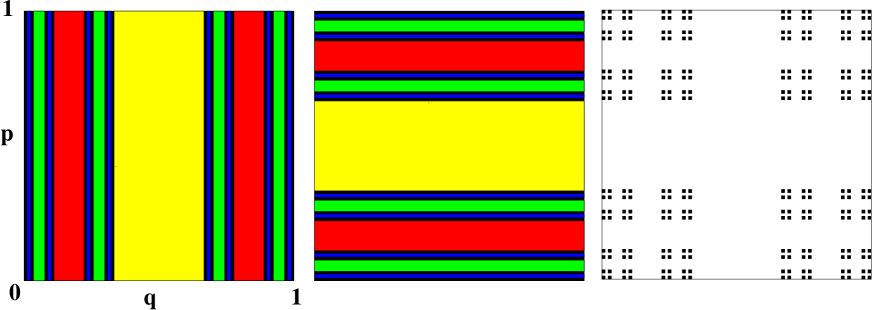
Figure 2. We show, from left to right, approximations of the in/outcoming tails $\Gamma_{-}$, $\Gamma_{+}$ and the trapped set $K$ for the open 3-baker $B_{3}$. On the left and central plots, each color corresponds to points escaping at the same time.

In analogy with (1.6), we also define the trapped set $K=\Gamma_{+}\cap\Gamma_{-}$ and, for any point $x\in K$, its stable and unstable manifolds $W_{\pm}(x)$. In the case of the open 3-baker $B_{3}$, we easily check that

$$\mu\stackrel{{\scriptstyle\rm{def}}}{{=}}\dim\Gamma_{-}\cap W_{+}=\dim\Gamma_{+}\cap W_{-}=\frac{1}{2}\dim K=\frac{\log 2}{\log 3}\,.$$

The quantization of the open map (2.6) is based on the quantization of the “closed” baker’s map $A_{3}$. That, in an outline, is done as follows [1, 13]. To any $N\in{\mathbb{N}}$ we associate a space ${\mathcal{H}}_{N}\simeq{\mathbb{C}}^{N}$ of quantum states on the torus. The components $\psi_{j}$, $j\in{\mathbb{Z}}_{N}=\left\{\,0,\ldots,N-1\,\right\}$ of a state $\psi\in{\mathcal{H}}_{N}$ are the amplitudes of $\psi$ at the positions $q=q_{j}=(j+\frac{1}{2})/{N}$, and we will sometimes use Dirac’s notation $\psi_{j}=\langle q_{j}|\psi\rangle$. The choice of these “half-integers positions” is justified by the parity symmetry $q\to 1-q$ they satisfy [13], and is further explained in §3. The scalar product on ${\mathcal{H}}_{N}$ is the standard one on ${\mathbb{C}}^{N}$:

(2.8) $$\forall\psi,\phi\in{\mathcal{H}}_{N},\quad\langle\phi|\psi\rangle=\sum_{j=0}^{N-1}\overline{\phi}_{j}\,\psi_{j}\,.$$

A classical observable depending on $q\in{\mathbb{R}}/{\mathbb{Z}}$ only, $f=f(q)$, is obviously quantized as the multiplication operator

$$\forall\psi\in{\mathcal{H}}_{N},\quad[\operatorname{Op}_{N}(f)\psi]_{j}=f\left(\frac{j+1/2}{N}\right)\,\psi_{j}\,.$$

The discrete Fourier transform

(2.9) $$({\mathcal{G}}_{N})_{j,j^{\prime}}=N^{-1/2}\,e^{-2i\pi(j+\frac{1}{2})(j^{\prime}+\frac{1}{2})/N}\,,\quad j,j^{\prime}=0,\ldots,N-1\,$$

transforms a “position vector” $\psi_{j}=\langle q_{j}|\psi\rangle$ into the corresponding “momentum vector” $\langle p_{j}|\psi\rangle=({\mathcal{G}}_{N}\psi)_{j}$. The momenta are also quantized to values $p_{j}=(j+\frac{1}{2})/{N}$, $j=0,\ldots,N-1$. Comparing the definition (2.9) with the (standard) Fourier transform on ${\mathbb{R}}$,

$${\mathcal{F}}_{\hbar}u(p)=\frac{1}{\sqrt{2\pi\hbar}}\int_{\mathbb{R}}e^{-ipq/\hbar}u(q)dq\,,$$

we see that the effective Planck’s constant in the discrete model is $\hbar=(2\pi N)^{-1}$.

As a result, any observable $g=g(p)$ can be quantized as

$$\operatorname{Op}_{N}(g)\psi={\mathcal{G}}_{N}^{*}\,\text{diag}\Big{(}g\big{(}(j+1/2)/{N}\big{)}\Big{)}\,{\mathcal{G}}_{N}\,\psi\,.$$

The Weyl quantization on the torus generalizes this map $f\mapsto\operatorname{Op}_{N}(f)$ to any classical observable $f$, that is any (smooth) function on the torus, in such a way that a real observable $f$ is associated with self-adjoint operators, and

$$\frac{i}{\hbar}[\operatorname{Op}_{N}(f),\operatorname{Op}_{N}(g)]=\operatorname{Op}_{N}(\{f,g\})+{\mathcal{O}}(\hbar^{2})\,.$$

Let us now consider the following family of unitary operators on ${\mathcal{H}}_{N}$, where $N$ is taken as a multiple of $3$:

(2.10) $$\widehat{A}_{3,{\rm pos}}=A_{3,N}\stackrel{{\scriptstyle\rm{def}}}{{=}}{\mathcal{G}}_{N}^{*}\left(\begin{array}[]{lll}{\mathcal{G}}_{N/3}&\ 0&\ 0\\ \ 0&{\mathcal{G}}_{N/3}&\ 0\\ \ 0&\ 0&{\mathcal{G}}_{N/3}\end{array}\right)\,.$$

Since ${\mathcal{G}}_{N}$ exchanges position and momentum, the mixed momentum-position representation of $\widehat{A}_{3}$ is given by the matrix

$$\widehat{A}_{3,{\rm mom-pos}}={\mathcal{G}}_{N}\,A_{3,N}=\left(\begin{array}[]{ccc}{\mathcal{G}}_{N/3}&\ 0&\ 0\\ \ 0&{\mathcal{G}}_{N/3}&\ 0\\ \ 0&\ 0&{\mathcal{G}}_{N/3}\end{array}\right)\,.$$

In terms of the quantized positions $q_{j}$ and momenta $p_{k}$, the entries of this matrix are given by

$$\big{(}\widehat{A}_{3,{\rm mom-pos}}\big{)}_{k\,j}=\langle p_{k}|\widehat{A}_{3}|q_{j}\rangle=\frac{1}{\sqrt{2\pi\hbar}}\ \exp\left(-\frac{i}{\hbar}(3q_{j}-\ell)\big{(}p_{k}-\frac{\ell}{3}\big{)}\right)\,,$$

$$\frac{\ell}{3}\leq q_{j}<\frac{\ell+1}{3}\,,\quad\frac{\ell}{3}\leq p_{k}<\frac{\ell+1}{3}\,,\quad\ell=0,1,2\,,$$

and zero otherwise. One can then observe [1] that for $\ell=0,1,2$, the function $S_{\ell}(p^{\prime},q)=(3q-\ell)(p^{\prime}-\ell/3)$ generates the canonical map $(q,p)\mapsto(q^{\prime},p^{\prime})=(3q-\ell,p/3+\ell/3)$ on the domain $\{q,p^{\prime}\in[\ell/3,(\ell+1)/3)\}$, that is, the map $A_{3}$ (2.5) on this domain. The matrix elements $\langle p_{k}|\widehat{A}_{3}|q_{j}\rangle$ therefore exactly correspond to the Van Vleck semiclassical formula associated with the map $A_{3}$. For this reason (and the unitarity of $\widehat{A}_{3}$), the operator $\widehat{A}_{3}$ was considered a good quantization of $A_{3}$ by Balazs and Voros. A more precise description of the correspondence between $A_{3}$ and $\widehat{A}_{3}$, including the role played by the discontinuities of $A_{3}$, is explained in [12, §4.4].

To quantize the open baker $B_{3}$ (2.6), we truncate the unitary operator $\widehat{A}_{3}$ using the quantum projector on the domain ${\mathcal{D}}$, $\Pi_{{\mathcal{D}}}\stackrel{{\scriptstyle\rm{def}}}{{=}}\operatorname{Op}_{N}({\mathchoice{1\mskip-4.0mu{\rm{l}}}{1\mskip-4.0mu{\rm{l}}}{1\mskip-4.5mu{\rm{l}}}{1\mskip-5.0mu{\rm{l}}}}_{{\mathcal{D}}})$ [14]: in the position basis, we get

(2.11) $$\widehat{B}_{3,{\rm pos}}=B_{3,N}\stackrel{{\scriptstyle\rm{def}}}{{=}}A_{3,N}\,\Pi_{{\mathcal{D}}}={\mathcal{G}}_{N}^{*}\left(\begin{array}[]{ccc}{\mathcal{G}}_{N/3}&0&\ 0\\ \ 0&0&\ 0\\ \ 0&0&{\mathcal{G}}_{N/3}\end{array}\right)\,,\quad N\in 3{\mathbb{N}}\,.$$

This subunitary operator is a model for the quantization of a Poincaré map of an open chaotic system [14]. The semiclassical régime corresponds to the limit $N\to\infty$. Similarly, the quantum open map associated with the 5-baker $B_{5}$ (2.7) is given by the sequence of matrices:

(2.12) $$B_{5,N}\stackrel{{\scriptstyle\rm{def}}}{{=}}{\mathcal{G}}_{N}^{*}\left(\begin{array}[]{ccccc}0&0&0&0&0\\ 0&{\mathcal{G}}_{N/5}&0&0&0\\ 0&0&0&0&0\\ 0&0&0&{\mathcal{G}}_{N/5}&0\\ 0&0&0&0&0\end{array}\right)\,,\quad N\in 5{\mathbb{N}}\,.$$

Let us now describe the correspondence between the resonances of a Schrödinger operator $\widehat{H}$, and the eigenvalues of our subunitary open quantum maps $B_{3,N}$ or $B_{5,N}$ (denoted generically by $B_{N}$).

Since $B_{N}$ is obtained by truncating the unitary propagator $A_{N}$, it is natural to consider the family of truncated Schrödinger propagators $\chi\,e^{-it\widehat{H}/\hbar}\,\chi$, where $\chi(q)$ is a cutoff function on some compact set supporting the scatterer. Although the precise eigenvalues of these propagators depend nontrivially on both $\chi$ and the time $t$, these propagators admit a long-time expansion in terms of the resonances $z_{j}$ of $\widehat{H}$ [3]. At an informal level, one may write

$$\chi\,e^{-it\widehat{H}/\hbar}\,\chi\sim\sum_{z_{j}\in\operatorname{Res}(\widehat{H})}\,e^{-itz_{j}/\hbar}\,\widehat{R}_{j}\,.$$

On the other hand, the iterated open quantum map $(B_{N})^{n}$ can obviously be expanded in terms of the eigenvalues $\lambda_{j}$ of $B_{N}$. For this reason, it makes sense to model the exponentials $e^{-iz_{j}/\hbar}$ by the eigenvalues $\lambda_{j}$ of our open quantum map $B_{N}$.

Upon this identification, the boxes in which we count resonances in (1.7), $[E-\rho\hbar,E+\rho\hbar]-i[0,\gamma\hbar]$, correspond to the regions

(2.13) $${\mathcal{A}}_{r,\vartheta,\rho}\stackrel{{\scriptstyle\rm{def}}}{{=}}\left\{\,1\geq|\lambda|\geq r\,,\ |\arg(\lambda\,e^{i\vartheta})|\leq\rho\,\right\}\,,\qquad r=\exp(-\gamma)\in(0,1)\,.$$

These analogies induce a conjectural fractal Weyl law for the quantum open bakers (2.6,2.7) which we now describe.

First of all, we consider the partial dimension of the trapped set of the open map $B$:

$$\mu=\frac{\dim K}{2}=\dim(\Gamma_{-}\cap W_{+})\,.$$

Then, for any $r\in(0,1)$, there should exist $C(r)\geq 0$ (a priori, depending on the map $B$) such that, in the semiclassical limit, the number of eigenvalues of $B_{N}$ in the sectors (2.13) behaves as

(2.14) $$\#\left\{\,\lambda\in\operatorname{Spec}(B_{N})\cap{\mathcal{A}}_{r,\vartheta,\rho}\,\right\}\simeq\ \frac{\rho}{2\pi}\,C(r)\,N^{\mu}\,\qquad N\to\infty\,.$$

The angular dependence ${\rho}/({2\pi})$ on the RHS means that the distribution of eigenvalues is expected to be asymptotically angular-symmetric.

In [15], the quantum 2-baker $A_{2,N}$ was decomposed into the block ${\mathcal{G}}_{N}^{*}\begin{pmatrix}{\mathcal{G}}_{N/2}&0\\ 0&0\end{pmatrix}$ and the complementary one. The spectral determinant for the unitary map, $\det(1-zA_{2,N})$, was then expanded in terms of these blocks. Although the classical open map associated with each block is quite simple (all points except a fixed one eventually escape), the spectrum of each block was found to be rather complex, and quite different from semiclassical predictions.

A scaling of the type (2.14) was conjectured in [18] for another chaotic map, namely the open kicked rotator. This conjecture was then tested numerically, and a good agreement was observed. The scaling law $N^{\mu}$ was explained heuristically by counting the number of quantum states in an $\hbar$-neighbourhood of the incoming tail $\Gamma_{-}$ (so that $\mu$ was effectively the dimension of $\Gamma_{-}$). For the kicked rotator, the fractal exponent $\mu$ was not known analytically, and the authors related it to the mean dwell time of the dynamics, that is, the average time spent in the cavity before leaving it: $\mu\approx 1-(\lambda\tau_{\rm dwell})^{-1}$ ($\lambda$ is the mean Lyapounov exponent). For our open baker’s maps $B_{3}$, the dwell time is $\tau_{\rm dwell}=3$, so the above formula is not valid: $\log 2/\log 3\neq 1-1/(3\log 3)$. However, the above formula should give a good approximation of $\mu$ for a system with a large dwell time (that is, a small opening).

In §3 we provide numerical evidence for the validity of (2.14) in the case of the open 5-baker $B_{5}$ (2.7), at least when taking $N$ along geometric subsequences. In §4.2 we then construct a related quantum model, for which we can prove this Weyl law and calculate $C(r)$ explicitly for inverse Planck’s constants of the form $N=5^{k}$, $k\in{\mathbb{N}}$.

3. Numerical results

We numerically computed the spectra of several open baker’s maps; in [12, §5] we showed the numerical results concerning the $3$-baker $B_{3}$ (2.6). For a change, we will discuss here the open $5$-baker (2.7), quantized in (2.12). For this open map, the partial dimension of the repeller is $\mu=\log 2/{\log 5}=0.4306765...$ Compared to the 3-baker, this smaller exponent implies that the spectrum of $\widehat{B}_{5}$ is expected to be much sparser than that of $\widehat{B}_{3}$. For this reason, we will represent the spectra using a logarithmic scale (see Fig. 4), and consider regions ${\mathcal{A}}_{r,\vartheta,\rho}$ for values of $r$ ranging from $r=0.5$ down to about $r=0.001$.

Let us now briefly explain the choice of “half-integer quantization” for the quantum positions and momenta [13]. The open map $B_{5}$ is symmetric with respect to the parity transformation $\Pi(q,p)=(1-q,1-p)$: $\Pi\circ B_{5}=B_{5}\circ\Pi$. The choice of quantization is made so that the associated quantum map $\widehat{B}_{5}$ also possess this symmetry, that is, it commutes with the quantum parity operator $\widehat{\Pi}$ defined as $\widehat{\Pi}|q_{j}\rangle=-|1-q_{j}\rangle=-|q_{N-1-j}\rangle$. We can then separately diagonalize the even and odd parts

$$\widehat{B}_{5,{\rm{ev}}}=\widehat{B}_{5}\circ({1+\widehat{\Pi}})/{2}\ \text{ and }\ \widehat{B}_{5,{\rm{odd}}}=\widehat{B}_{5}\circ({1-\widehat{\Pi}})/{2}\,.$$

Both these operators have rank $N/5$: together, they give the full nontrivial spectrum of $\widehat{B}_{5}$. We checked that the odd spectrum has the same characteristics as the even one, so we only describe the properties of the latter. It is expected to satisfy the following fractal law (consequence of (2.14)):

(3.1) $$n(N,r)\stackrel{{\scriptstyle\rm{def}}}{{=}}\#\{\operatorname{Spec}(B_{5,N,{\rm ev}})\cap{\mathcal{A}}_{r}\}\simeq C(r)\,(N/5)^{\log 2/\log 5}\,,\quad{\mathcal{A}}_{r}=\{|\lambda|>r\}\,,\quad N\to\infty\,.$$

The simplest set of $N$’s to test this fractal Weyl law is given by geometric sequences of the type $\{N_{o}\times 5^{k},\ k=0,1,\ldots\}$: the law (3.1) means that the number of eigenvalues doubles when $k\to k+1$. In table 1 we give some of the numbers $n(N,r)$ along the sequence $N\in\{5^{k}\times 20\}$, for some selected values of $r$.

$N=20\times 5^{k}$	$r=0.5$	$r=0.1$	$r=0.05$	$r=0.01$	$r=0.05$	$r=0.001$
$k=0$	4	10	10	13	14	16
$k=1$	7	19	19	25	27	35
$k=2$	15	36	36	48	55	122
$k=3$	30	69	69	104	216	402

Table 1. Number of even-parity eigenvalues of $B_{5,N}$ in $\{|\lambda|>r\}$, for $N$ along the sequence $\{20\times 5^{k}\}$.

Along each column with $r\geq 0.01$, the numbers approximately double at each step $k\to k+1$, which seems to confirm the law (3.1). The fact that this law fails for the small radii $r=0.005,\,0.001$ may be explained as follows: according to (3.1), when $N$ is large the huge majority of the $N/5$ eigenvalues of $B_{5,N,{\rm ev}}$ must be contained within an asymptotically small neighbourhood of the origin; if ${\mathcal{A}}_{r}$ intersects this neighbourhood, the law (3.1) necessarily fails, since the counting function is proportional to $N$ instead of $N^{\mu}$. For the values of $N$ listed in the table, this small region seems to be of radius $\gtrsim 0.005$, explaining the departure from the fractal law in the last two columns.

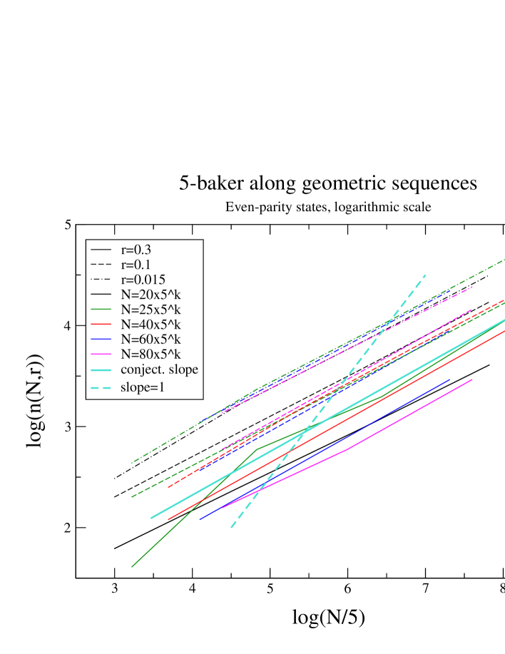
Figure 3. Checking the $N$-dependence of $n(N,r)$ for various values of $r$ and $N$ along geometric sequences $\{N_{o}\times 5^{k}\}$. We also show (thick line) the conjectured slope $\log 2/\log 5$, and give for comparison the slope $1$ (thick dashed).

To further test the validity of the fractal law (3.1), we choose a set of values of $r$, and study the $N$-dependence of $n(N,r)$, for $N$ taken along several geometric sequences, generalizing the above table. In Fig. 3, we plot this dependence in logarithmic scale for $r=0.3$ (full lines), $r=0.1$ (dashed lines), $r=0.015$ (dot-dashed lines). Different geometric sequences are represented by a different colors. For almost all pairs $(N_{o},r)$ the points are almost aligned, and the slope is in very good agreement with the conjectured one $\mu=\log 2/\log 5$. The less convincing data are the ones related to $r=0.3$: for this radius, the numbers $n(N,r)$ are still quite small, so that fluctuations are much more visible than for the smaller radii. We expect this effect to disappear for larger values of $N$.

In Fig. 3 the height of the curves does not only depend on $r$, but also on the sequence $\{N_{o}\times 5^{k}\}$ considered, especially for $r=0.3$.

Figure 4. Even-parity spectra of the quantum baker’s maps $B_{5,N}$, along geometric sequences $N=N_{o}\times 5^{k}$. The eigenvalues are represented on a logarithmic scale ($\arg\lambda/2\pi$ against $\log|\lambda|$). The dimensions indicated correspond to $N/5$.

To investigate this apparent contradiction with (3.1) we plot in Fig. 4 the even spectra of $B_{5,N}$ along 3 different geometric sequences. These plots suggest that, along a given geometric sequence, the eigenvalue density increases with $N$ uniformly with respect to $\phi=\arg\lambda$, but very nonuniformly with respect to $|\lambda|$. We see that some regions $\{r_{0}<|\lambda|<r_{1}\}$ remain empty even for large values of $N$. The presence of gaps was already noticeable when comparing the second and third columns of table 1: obviously, for $N=20\times 5^{k}$, there were no eigenvalues in the annulus $\{0.05<|\lambda|<0.1\}$, which is confirmed visually in Fig. 4 (bottom). This non-uniform dependence on $|\lambda|$ implies that the profile function $C(r)$ is nontrivial.

The spectra for the two other geometric sequences also shows the presence of gaps, but the gaps differ from one geometric sequence to the other. This observation also contradicts the law (3.1).

   

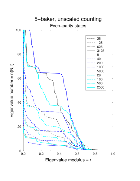
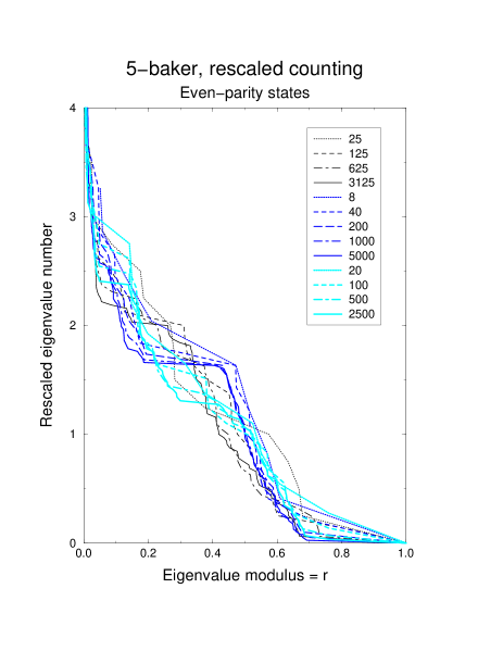
Figure 5. On the left, we plot $n(N,r)$ as functions of $r\in(0,1)$. The numbers in the legend are $N/5$. On the right we have multiplied $n(N,r)$ by the factor $(N/5)^{-{\log 2}/{\log 5}}$.

In spite of these problems we nevertheless attempt to compute the profile function $C(r)$ appearing in (3.1). Fig. 5 (left) shows $n(N,r)$ as functions of $r\in(0,1)$, for $N$ along the same three geometric sequences (each one corresponding to a given color/width). We then rescale the vertical coordinate of each curve by the factor $(N/5)^{-{\log 2}/{\log 5}}$, and plot the rescaled curves in Fig. 5 (right). From far away, these rescaled curves are fairly superposed on each other, which shows that the conjectured scaling (3.1) is approximately correct. Yet, a closer inspection shows that a much better convergence to a single function occurs along each individual geometric sequence. For instance, the curves for $N=8\times 5^{k}$ “pointwise” converge to the last one along this sequence ($N/5=5000$), which has a plateau on $\{0.2\lesssim r\lesssim 0.4\}$ corresponding to a spectral gap. The curves of the two other sequences seem to converge as well, with plateaux on different intervals.

In the case of the open kicked rotator studied in [18] the rescaled curves $n(N,r)$ are more or less superposed, therefore defining a profile function $C(r)$. The authors claim that this function corresponds reasonably well with a prediction of random matrix theory [24]. Our results for the 5-baker’s map contradict this universality: there does not seem to be a global profile function $C(r)$, but a family of such functions, which depend on the geometric sequence $\{N_{o}\times 5^{k}\}$, which could be denoted by $C(N_{o},r)$. The law (3.1) needs to be adapted by restricting $N$ to geometric sequences, which yields the following empirical scaling law:

For any $N_{o}>0$ and $r\in(0,1)$, there exists $C(N_{o},r)\geq 0$ such that, for $N$ along $\{N_{o}\times 5^{k}\}$ and $k\to\infty$,

(3.2) $$\#\left\{\,\lambda\in\operatorname{Spec}(B_{N})\cap{\mathcal{A}}_{r,\vartheta,\rho}\,\right\}\simeq\ \frac{\rho}{2\pi}\,C(N_{o},r)\,N^{\mu}\,,$$

where ${\mathcal{A}}_{r,\vartheta,\rho}$ is given by (2.13). In Fig. 5 the different profile functions are uniformly bounded, $C_{1}(r)\leq C(N_{o},r)\leq C_{2}(r)$, for some envelope functions $0\leq C_{1}(r)\leq C_{2}(r)$.

This weakening of (2.14) to geometric sequences makes sense for baker’s maps of the form $B_{3}$, $B_{5}$, which each have a uniform integer expansion factor, leading to number-theoretic properties. In the case of a nonlinear open chaotic map (as the open kicked rotator of [18]), there is no reason for geometric sequences to play any role, so we expect (2.14) to hold in that case.

4. A computable model

Because we are unable to analyze the spectra of the quantum bakers $B_{N}$ rigorously, we introduce simplified models. In the case of the 3-baker, we observe (see Fig. 6, left) that the largest matrix elements are maximal along the “tilted diagonals”

(4.1) $$(n,m)=(3l+\epsilon,l+\ell N/3),\quad\text{with}\quad l\in\{0,\ldots,N/3-1\},\quad\ell\in\{0,2\},\quad\epsilon\in\{0,1,2\}\,.$$

These “diagonals”correspond to a discretization of the the map $B_{3}$ projected on the position axis. Away from them, the coefficients do not decrease very fast due to the Gibbs phenomenon (diffraction). The elements on the “diagonals” have moduli $1/\sqrt{3}+{\mathcal{O}}(1/N)$ and their phases only depend on $\ell,\,\epsilon$ in the above parametrization. Our simplified model is obtained by keeping only the elements on the “diagonals” (see Fig. 6, right), set their moduli to $1/\sqrt{3}$ and shift their phases by $\pi/2$ (for convenience). Using the parametrization (4.1), we get:

(4.2) $$({\widetilde{B}}_{3,N})_{n\,m}=\frac{1}{\sqrt{3}}\,\exp\big{(}\frac{2i\pi}{3}(\epsilon+1/2)(\ell+1/2)\big{)}\,.$$

For $N=9$ and using $\omega=e^{2\pi i/3}$, the matrix reads

$${\widetilde{B}}_{3,9}=\frac{\omega^{1/4}}{\sqrt{3}}\left(\begin{array}[]{lllllllll}1&0&0&0&0&0&\omega&0&0\\ \omega^{1/2}&0&0&0&0&0&\omega^{1/2}&0&0\\ \omega&0&0&0&0&0&1&0&0\\ 0&1&0&0&0&0&0&\omega&0\\ 0&\omega^{1/2}&0&0&0&0&0&\omega^{1/2}&0\\ 0&\omega&0&0&0&0&0&1&0\\ 0&0&1&0&0&0&0&0&\omega\\ 0&0&\omega^{1/2}&0&0&0&0&0&\omega^{1/2}\\ 0&0&\omega&0&0&0&0&0&1\end{array}\right)\,.$$

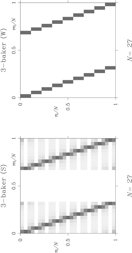
Figure 6. Matrices $B_{3,27}$ (left) and its toy model ${\widetilde{B}}_{3,27}$ (right). The gray scale represents the modulus of the matrix elements (white$=0$, black$=1$).

The matrix ${\widetilde{B}}_{3,N}$ can obviously not be considered as a “small perturbation” of $B_{3,N}$, since we removed many nonnegligible “off-diagonal” elements. Actually, by acting with ${\widetilde{B}}_{3,N}$ on Gaussian coherent states, one realizes that these matrices do not quantize the open 3-baker $B_{3}$ (2.6), but rather a more complicated multivalued map ${\widetilde{B}}_{3}$, built upon $B_{3}$ as follows:

(4.3) $$\forall(q,p)\in{\mathcal{D}}_{3},\quad{\widetilde{B}}_{3}(q,p)=\bigcup_{j=-1}^{1}\{B_{3}(q,p)+(0,j/3)\}\,.$$

We refer to [12, Proposition 6.1] for a precise statement. As opposed to $B_{3}$, the multivalued map (4.3) is no longer obtained by truncating a canonical transformation, but it comes from three different transformations. ${\widetilde{B}}_{3}$ can be considered as a model of propagation with ray splitting. Another interpretation is given by considering a Markov process with probabilities $P(x^{\prime},x)$ being allocated at each step to the image points $x^{\prime}$ of $x$. Explicitly, the probabilities take the form

$$P(x^{\prime},x)=f\left(\frac{3p^{\prime}-[3q]-1/2}{3}\right)\,,\ \ f(t)=\left(\frac{\sin(3\pi t)}{3\sin(\pi t)}\right)^{2}\,,\ \ x=(q,p)\,,\ x^{\prime}=(q^{\prime},p^{\prime})\,,$$

so that for each $x\in{\mathcal{D}}_{3}$, the sum of the weights associated with the three images of $x$ is indeed $1$.

Some of the characteristics of the dynamics remain the same as for $B_{3}$. The local dynamics of each branch is the same, and ${\widetilde{B}}_{3}$ sends all points in ${\mathbb{T}}^{2}\setminus{\mathcal{D}}_{3}$ to infinity. One can define incoming and outgoing tails for ${\widetilde{B}}_{3}$ (see §2). As opposed to the case of $B_{3}$, these tails are not symmetrical any more: $\Gamma_{-}={\mathcal{C}}_{3}\times[0,1)$, $\quad\Gamma_{+}={\mathbb{T}}^{2}$. Yet, these formulas are slightly misleading. The second one comes from the fact that any point $x\in{\mathbb{T}}^{2}$ has two preimages through ${\widetilde{B}}_{3}$, namely $x_{0}=(q/3,3p),\ x_{2}=((q+2)/3,3p)$, so no point ever escapes to infinity in the past. However, to these preimages are associated the respective weights $P(x,x_{0})$, $P(x,x_{2})$, the sum of which is generally $<1$: there is thus a loss of probability through ${\widetilde{B}}_{3}^{-1}$, which is not accounted for by the definition of $\Gamma_{+}$.

In the next section we will show that the matrices ${\widetilde{B}}_{3,N}$ can nonetheless be interpreted as quantizations of the original open baker $B_{3}$, as long as one switches to a different notion of quantization, derived from a different type of Fourier transform (the Walsh-Fourier transform).

Families of unitary matrices ${\widetilde{A}}_{2,N}$ with a structure similar to ${\widetilde{B}}_{3,N}$ have already been proposed as an alternative quantization of the 2-baker’s map $A_{2}$ [16]. These matrices can also closely related with the “semiquantum bakers” introduced in [15]. In the context of quantum graphs (a recently popular model for quantum chaos), unitary matrices similar with ${\widetilde{A}}_{2,N}$ (but with random phases) occur as “unitary transfer matrices” associated with binary graphs [21]. In this framework, the matrix ${\widetilde{A}}_{2,N}$ would correspond to a graph with very degenerate bond lengths. In this framework, the matrix ${\widetilde{B}}_{3,N}$ is directly related with a classical transfer matrix defined by $({\mathcal{B}}_{3,N})_{j\,j^{\prime}}=\big{|}({\widetilde{B}}_{3,N})_{j\,j^{\prime}}\big{|}^{2}$, which represents the classical Markov process on the graph. In our case, this transfer matrix is the discretized version of the transfer (Perron-Frobenius) operator associated with the open map $B_{3}$.

4.1. The Walsh model interpretation of ${\widetilde{B}}_{3,N}$.

In this section, we represent the matrices ${\widetilde{B}}_{3,N}$ in a way suitable for their spectral analysis. This can be done only in the case where $N$ is a power of $3$. This representation is connected with the Walsh model of harmonic analysis.

The latter originally appeared in the context of fast signal processing [8]. The major advantage of Walsh harmonic analysis (compared with the usual Fourier analysis) is the possibility to strictly localize wave packets simultaneously in position and in momentum. For our problem, this has the effect to remove the diffraction problems due to the discontinuities of the classical map, which spoil the usual semiclassics [15].

A recent preprint [10] analyzes some special eigenstates of the “standard” quantum 2-baker, using the Walsh-Hadamard transform (which slightly differs from the Walsh transform we give below) as a “filter”. We are doing something different here by constructing our simplified model ${\widetilde{B}}_{3,N}$ from the Walsh transform, as $B_{3,N}$ was constructed from the discrete Fourier transform (see §2).

We first select the expanding coefficient of the baker’s map, which we denote by $D\in{\mathbb{N}}$ (the map (2.6) is associated with $D=3$, the map (2.7) with $D=5$). Once this is done, we will restrict ourselves to the values of $N$ along the geometric sequence $\{N=D^{k}\,,k\in{\mathbb{N}}\}$. In this case, the Hilbert space can be naturally decomposed as a tensor product of $k$ spaces ${\mathbb{C}}^{D}$:

(4.4) $${\mathcal{H}}_{N}=({\mathbb{C}}^{D})_{1}\otimes({\mathbb{C}}^{D})_{2}\otimes\cdots\otimes({\mathbb{C}}^{D})_{k}\,.$$

This decomposition appears naturally in the context of quantum computation, where each ${\mathbb{C}}^{D}$ represents a “quantum $D$-git”, that is, a quantum system with $D$ levels. Here, we realize this decomposition using the basis of position eigenstates $|q_{j}\rangle$ of ${\mathcal{H}}_{N}$ (see [16] for the case $D=2$). Indeed, each quantum position $q_{j}=({j+1/2})/{N}$, $j\in{\mathbb{Z}}_{D^{k}}=\{0,\ldots,N-1\}$ is in one-to-one correspondence with a word $\boldsymbol{\epsilon}=\epsilon_{1}\epsilon_{2}\cdots\epsilon_{k}$ made of symbols ($D$-gits) $\epsilon_{\ell}=\epsilon_{\ell}(j)\in{\mathbb{Z}}_{D}$:

(4.5) $$j=\sum_{\ell=1}^{k}\epsilon_{\ell}\,D^{k-\ell}\,.$$

The usual order for $j\in{\mathbb{Z}}_{D^{k}}$ corresponds to the lexicographic order for the symbolic words $\boldsymbol{\epsilon}\in({\mathbb{Z}}_{D})^{k}$. Associating to each $D$-git a $D$-dimensional vector space $({\mathbb{C}}^{D})_{\ell}$ with canonical basis $\{e_{0},e_{1},\ldots,e_{D-1}\}$, the position eigenstate $|q_{j}\rangle\in{\mathcal{H}}_{N}$ can be decomposed as

(4.6) $$|q_{j}\rangle=e_{\epsilon_{1}}\otimes e_{\epsilon_{2}}\otimes\cdots\otimes e_{\epsilon_{k}}\,.$$

This identification realizes the tensor product decomposition (4.4).

The Fourier transforms ${\mathcal{G}}_{N}$ (2.9), and the simpler one without the $1/2$ shift,

(4.7) $$({\mathcal{F}}_{N})_{j\,j^{\prime}}=\frac{e^{-2i\pi j\,j^{\prime}/N}}{\sqrt{N}}\,,\quad j,j^{\prime}\in{\mathbb{Z}}_{N}\,,\ N=D^{k}\,,$$

are defined by applying the exponential function $x\mapsto e^{-2i\pi x}$ to the products

$$\frac{jj^{\prime}}{D^{k}}=\sum_{m=2-k}^{k}D^{-m}\,\tilde{\epsilon}_{m}(jj^{\prime}),\quad\text{where}\quad\tilde{\epsilon}_{m}(jj^{\prime})=\sum_{\ell+\ell^{\prime}=m+k}\epsilon_{\ell}(j)\epsilon_{\ell^{\prime}}(j^{\prime})\,.$$

If we replace in (4.7) the exponential $e^{-2i\pi x}$ by the piecewise constant function $e_{D}(x)=\exp(-2i\pi[Dx]/D)$, and replace each $\tilde{\epsilon}_{m}(jj^{\prime})$ by its value $\epsilon_{m}(jj^{\prime})$ modulo $D$, we obtain the matrix element

(4.8) $$\begin{split}({\mathcal{V}}_{k})_{j\,j^{\prime}}&\stackrel{{\scriptstyle\rm{def}}}{{=}}D^{-k/2}\,e_{D}\big{(}\sum_{m=2-k}^{k}D^{-m}\epsilon_{m}(jj^{\prime})\big{)}=D^{-k/2}\,\exp\big{(}-\frac{2i\pi}{D}\,\epsilon_{1}(jj^{\prime})\big{)}\\ &=\prod_{\ell=1}^{k}D^{-1/2}\,\exp\Big{(}-\frac{2i\pi}{D}\,\epsilon_{\ell}(j)\,\epsilon_{k+1-\ell}(j^{\prime})\Big{)}\,.\end{split}$$

The matrix ${\mathcal{V}}_{k}$ defines the Walsh transform in dimension $D^{k}$.

Because we have used the “half-integer” Fourier transform (2.9) to define our quantum baker’s map, we will need a slightly different version of Walsh transform, namely

$$({\mathcal{W}}_{k})_{j\,j^{\prime}}\stackrel{{\scriptstyle\rm{def}}}{{=}}\prod_{\ell=1}^{k}D^{-1/2}\,\exp\Big{(}-\frac{2i\pi}{D}\,\big{(}\epsilon_{\ell}(j)+1/2)\,(\epsilon_{k+1-\ell}(j^{\prime})+1/2\big{)}\Big{)}\,.$$

Both ${\mathcal{V}}_{k}$ and ${\mathcal{W}}_{k}$ preserve the tensor product structure (4.4): for any $v_{1},\ldots,v_{n}\in{\mathbb{C}}^{D}$,

(4.9) $${\mathcal{V}}_{k}(v_{1}\otimes\cdots\otimes v_{k})={\mathcal{F}}_{D}v_{k}\otimes\cdots\otimes{\mathcal{F}}_{D}v_{1}\,,\qquad{\mathcal{W}}_{k}(v_{1}\otimes\cdots\otimes v_{k})={\mathcal{G}}_{D}v_{k}\otimes\cdots\otimes{\mathcal{G}}_{D}v_{1}\,.$$

These expressions show that ${\mathcal{V}}_{k}$ and ${\mathcal{W}}_{k}$ are unitary.

Specializing the computations to $D=3$, we are now in position to define the toy model ${\widetilde{B}}_{3,N}$ (in the case $N=3^{k}$) as the “Walsh-quantization” of the 3-baker (2.6) (as opposed to the “standard” quantization of the multivalued map ${\widetilde{B}}_{3}$ (4.3)). Indeed, one can check that the matrix (4.2) can be expressed as

(4.10) $${\widetilde{B}}_{3,N}={\mathcal{W}}_{k}^{*}\left(\begin{array}[]{lll}{\mathcal{W}}_{k-1}&0&\ 0\\ \ 0&0&\ 0\\ \ 0&0&{\mathcal{W}}_{k-1}\end{array}\right)\,.$$

This formula is clearly the Walsh analogue of the definition (2.11) of the “standard” quantum open baker $B_{3,N}$. From this definition and (4.9), we see the action of $B_{3,N}$ on tensor products:

(4.11) $${\widetilde{B}}_{3,N}(v_{1}\otimes\cdots\otimes v_{k})=v_{2}\otimes\cdots\otimes v_{k}\otimes{\mathcal{G}}_{3}^{*}\pi_{0,2}v_{1}\,,\quad v_{j}\in{\mathbb{C}}^{3}\,,$$

where $\pi_{0,2}$ is the orthogonal projector (in ${\mathbb{C}}^{3}$) on ${\mathbb{C}}e_{0}\oplus{\mathbb{C}}e_{2}$.

4.2. Distribution of resonances

Figure 7. Eigenvalues of the matrices ${\widetilde{B}}_{3,N}$ for $N=3^{10}$ (triangles) and for $N=3^{15}$ (crosses), forming lattices in a logarithmic scale. The two horizontal lines correspond to the spectral radius $|z|=1$ (thin line) and the “peak multiplicity” $|z|=3^{-1/4}$ (thick line). Notice the difference of vertical scale compared with the spectra of Fig. 4.

Using (4.11) we can explicitly describe the spectrum of ${\widetilde{B}}_{3,N}$ for $N=3^{k}$. The computation is identical with [12, Section 6.2], so we only give the results. The generalized kernel of ${\widetilde{B}}_{3,N}$ is spanned by the position states $|q_{j}\rangle$ such that $\epsilon_{\ell}(j)=1$ for at least one index $1\leq\ell\leq k$. This corresponds to positions $q_{j}$ “far” from the Cantor set ${\mathcal{C}}_{3}$, so that the classical points $(q_{j},p)$ are sent to infinity at a time $n\leq k$. This kernel has dimension $3^{k}-2^{k}=N-N^{\log 2/\log 3}$.

The nonzero eigenvalues of ${\widetilde{B}}_{3,N}$ are given by the set (see Fig. 7)

$$\{\lambda_{+}\}\cup\{\lambda_{-}\}\cup\bigcup_{\ell=0}^{k-1}\bigcup_{p=1}^{k-1}\{e^{2i\pi\ell/k}\,\lambda_{+}^{1-p/k}\,\lambda_{-}^{p/k}\}\,,\quad\text{where}\ \lambda_{+}=1,\ \lambda_{-}=\frac{i}{\sqrt{3}}\,.$$

For each $p\in\{1,\ldots,k-1\}$, the $k$ eigenvalues of modulus $|\lambda_{-}|^{p/k}=3^{-p/2k}$ asymptotically have the same degeneracy $\binom{k}{p}/k$ as $k\to\infty$ (semiclassical limit), which shows that their distribution is circular-symmetric. Taking these multiplicities into account, we obtain the following Weyl law for the eigenvalues of ${\widetilde{B}}_{3,N}$ inside a region (2.13), along the sequence $N\in\{3^{k}\}$, $k\to\infty$:

(4.14) $$\begin{gathered}\#\left\{\,\operatorname{Spec}({\widetilde{B}}_{3,N})\cap{\mathcal{A}}_{r,\vartheta,\rho}\,\right\}\ =\frac{\rho}{2\pi}\,\,N^{\mu}\,(C(1,r)+o(1))\,\\ \mu=\dim(\Gamma_{-}\cap W_{+})=\frac{\log 2}{\log 3}\,,\qquad C(1,r)={\mathchoice{1\mskip-4.0mu{\rm{l}}}{1\mskip-4.0mu{\rm{l}}}{1\mskip-4.5mu{\rm{l}}}{1\mskip-5.0mu{\rm{l}}}}_{(0,3^{-1/4}]}(r)\,.\end{gathered}$$

The values $\lambda_{-}$, $\lambda_{+}$ in (4.14) are the nonzero eigenvalues of the matrix ${\mathcal{G}}_{3}^{*}\circ\pi_{0,2}$ appearing in (4.11). We used the notation $C(1,r)$ for the profile function to be consistent with our notations in (3.2), that is, to emphasize that this estimate is valid only along the sequence $N\in\left\{\,1\times 3^{k}\,\right\}$.

We notice that the spectrum of the classical transfer matrix ${\mathcal{B}}_{3,N}$ defined at the end of §4 is drastically different: this matrix admits one simple nontrivial eigenvalue $\lambda=2/3$ (interpreted as the classical escape rate), the rest of the spectrum lying in the generalized kernel. Therefore, the features of the quantum spectrum is intimately related with the oscillatory phases of ${\widetilde{B}}_{3,N}$ along the “diagonals”.

4.3. Conductance and Shot Noise

In this section, we consider an open baker’s map as a model of quantum transport through a “chaotic quantum dot”, that is a 2-dimensional cavity connected to the outside world through a certain number of “leads” carrying the current; each lead is connected to the cavity along a segment $L_{j}$ of the boundary (see Fig. 8), and the connection is assumed to be “perfect”: a particule inside the cavity which hits the boundary along $q\in L_{j}$ is completely evacuated to the lead. Therefore, the phase space domain $L_{j}\times[0,1)$ above this segment is a part of the “hole”, in the terminology of §2, whereas the remaining set $I=[0,1)\setminus(\cup L_{j})$ represents the boundary of the quantum dot, which lifts to the phase space domain ${\mathcal{D}}=I\times[0,1)$.

In the previous sections we have studied the open quantum map obtained by projecting a unitary quantum dynamics (called generically $U_{N}$) onto a subdomain ${\mathcal{D}}$ of the phase space: resonances were defined as the eigenvalues of $U_{N}\Pi_{{\mathcal{D}}}$. These resonances are supposed to represent the metastable quantum states inside the open quantum dot, after it has been opened. In the present section, we want to study another aspect of the open system, namely the “transport” through the dot, using the formalism of [22]. We will focus on the case where the opening $L$ splits into two segments $L=L_{1}\cup L_{2}$, and we study the transmission matrix from the lead $L_{1}$ to the lead $L_{2}$.

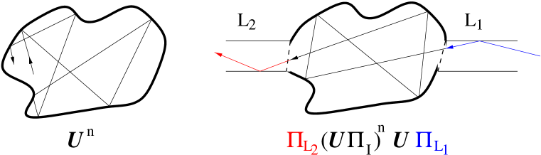
Figure 8. Closed and open chaotic cavity. On the left, a (bounded) trajectory is schematically associated with a power of the unitary quantum propgator ($n$ represents the number of bounces). On the right, a “transmitting” trajectory is associated with a term of the matrix (4.15).

Once we are given, on one side, the quantum map $U_{N}$ associated with the closed dynamics inside the “cavity”, on the other side, the projectors on the leads $\Pi_{L_{i}}$ and on the “interior” $\Pi_{I}=\Pi_{\mathcal{D}}$, the transmission matrix (from $L_{1}$ to $L_{2}$) is defined as the block

(4.15) $$t(\vartheta)=\sum_{n\geq 1}e^{in\vartheta}\,\Pi_{L_{2}}\,U_{N}\,(\Pi_{I}U_{N})^{n-1}\,\Pi_{L_{1}}\,.$$

The parameter $\vartheta\in[0,2\pi)$ is the “quasi-energy” of the particles. According to Landauer’s theory of coherent transport, each eigenvalue $T_{i}(\vartheta)$ of the matrix $t(\vartheta)t^{*}(\vartheta)$ corresponds to a “transmission channel”. The dimensionless conductance of the system is then given by

(4.16) $$g(\vartheta)=\operatorname{tr}\big{(}t(\vartheta)\,t^{*}(\vartheta)\big{)}\,.$$

A transmission channel is “classical” if the eigenvalue $T_{i}$ is very close to unity (perfect transmission) or close to zero (perfect reflection). The intermediate values characterize “nonclassical channels” (governed by strong interference effects). The number number of the latter can be estimated by the noise power

(4.17) $$P(\vartheta)=\operatorname{tr}\Big{(}t(\vartheta)t^{*}(\vartheta)\big{(}Id-t(\vartheta)t^{*}(\vartheta)\big{)}\Big{)}\,,$$

or equivalently the Fano factor, $F={P}/{g}$. It is sometimes necessary to perform an ensemble averaging over $\vartheta$ to obtain significant results [22]. However, for the model we study here, these quantities will depend very little on $\vartheta$.

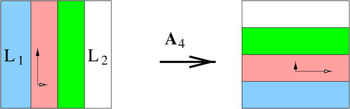
Figure 9. 4-baker’s map modeling the chaotic cavity. The left- and rightmost vertical strips correspond to the two openings (“leads”).

The closed quantum dot will be modeled by the following quantum map: we consider the 4-baker’s map $A_{4}$ and quantize it using the Walsh transform ${\mathcal{V}}_{k}$ (4.8) with $D=4$. In dimension $N=4^{k}$, our unitary propagator is therefore

$$U_{N}={\widetilde{A}}_{4,N}={\mathcal{V}}_{k}^{*}\left(\begin{array}[]{llll}{\mathcal{V}}_{k-1}&0&0&0\\ 0&{\mathcal{V}}_{k-1}&0&0\\ 0&0&{\mathcal{V}}_{k-1}&0\\ 0&0&0&{\mathcal{V}}_{k-1}\end{array}\right)\,.$$

We attach the leads on the intervals $L_{1}=[0,1/4]$ and $L_{2}=[3/4,1]$: this way, the projectors $\Pi_{L_{i}}$ as well as the projector $\Pi_{I}=Id-\Pi_{L_{1}}-\Pi_{L_{2}}$ can be represented as tensor product operators:

$$\Pi_{L_{1}}=\pi_{0}\otimes Id_{4}\otimes Id_{4}\otimes\cdots\,,\quad\Pi_{L_{2}}=\pi_{3}\otimes Id_{4}\otimes\cdots\,,\quad\Pi_{I}=\pi_{I}\otimes Id_{4}\otimes\cdots\,.$$

Here $\pi_{i}$ is the orthogonal projector on the basis state $e_{i}$ of ${\mathbb{C}}^{4}$, and $\pi_{I}=\pi_{1}\oplus\pi_{2}$. This tensor action, together with the action of ${\widetilde{A}}_{4,N}$ (analogous to (4.11)), allow us to compute all quantities explicitly.

The spectrum of the “inside” propagator for this model, ${\widetilde{B}}_{4,N}={\widetilde{A}}_{4,N}\Pi_{I}$, satisfies a fractal Weyl law of the type (4.14) along the sequence $N=4^{k}$, with exponent $\mu=\log 2/\log 4=1/2$, and profile $C(1,r)={\mathchoice{1\mskip-4.0mu{\rm{l}}}{1\mskip-4.0mu{\rm{l}}}{1\mskip-4.5mu{\rm{l}}}{1\mskip-5.0mu{\rm{l}}}}_{[0,2^{-3/4}]}(r)$.

For this model and in the semiclassical limit $k\to\infty$, we could compute the dimensionless conductance (4.16). The computation [12, §7.2] requires to control the time evolution up to $n=Ck$ for some $1<C<2$: this is of the order of the Ehrenfest time $\tau_{E}=k$ for the system. For any $\vartheta$ we obtain

(4.18) $$g(N=4^{k},\vartheta)=\frac{4^{k-1}}{2}(1+o(2^{-k}))=\frac{N/4}{2}\,(1+o(1))\,,\qquad k\to\infty\,.$$

Here $N/4$ is the number of transmission channels from $L_{1}$ to $L_{2}$, that is the rank of the matrix $t(\vartheta)$. We see that, as could be expected, approximately one half of the scattering channels get transmitted from one lead to the other, the other half being reflected back.

Asymptotics for the shot noise (4.17) (which counts the “nonclassical” transmission channels”) are more interesting and again independent of $\vartheta$:

(4.19) $$P(N=4^{k},\vartheta)=2^{k-1}\,\Big{(}\frac{11}{80}+{\mathcal{O}}(e^{-Ck})\Big{)}=\frac{11}{80}\,(N/4)^{\mu}\,(1+o(1))\,,\quad k\to\infty\,.$$

Here $\mu=1/2$ is the dimension appearing in the fractal Weyl law for the resonances. A similar fractal law for the shot noise had been observed in [22] in the case of the quantum kicked rotator; the power law $N^{\mu}$ for the number of nonclassical channels was explained there through a study of the dynamics up to the Ehrenfest time.

The constant $11/80$ in (4.19) gives the average “shot noise” per nonclassical transmission channel. This number is close to the random matrix theory prediction for this quantity, namely $1/8$ [7, 22]. The precise number $11/80$ certainly depends on which baker’s map one starts from, and which quantization one uses. For instance, we did not check whether the “half-integer” Walsh quantization of the 4-baker leads to the same prefactor, but we expect the result to be close to it. It would be interesting to actually check the full distribution for the transmission eigenvalues $T_{i}$, and compare it with the prediction of random matrix theory [7].

The near agreement with random matrix theory is in contrast with the fact that the semiclassical resonance spectrum of the propagator ${\widetilde{B}}_{4,N}$ inside the dot is very different from that of a random subunitary matrix. Somehow, the matrix $t(\vartheta)$, obtained by summing iterates of ${\widetilde{B}}_{4,N}$, has acquired some “randomness”, as far as the distribution of its singular values is concerned.

The transport properties of chaotic cavities has also been studied within the framework of quantum graphs. The shot noise (4.17) could be semiclassically estimated in the case of a “star graph”, by summing over transmitting trajectories on the graph [17] (they studied the case of “small openings”). The authors show that one needs to take into account the “action correlations” between different trajectories, in order to reproduce the random matrix result. As mentioned before, the matrix ${\widetilde{A}}_{4,N}$ can be interpreted as the unitary transfer matrix for a different type of graph [21], with bonds having degenerate lengths. Somehow, our use of the tensor product structure implicitly takes into account the action correlations for this particular graph.

5. Conclusions

Quantum open baker’s maps provide a simple and elegant model for the study of quantum resonances of open chaotic systems. The numerical investigation of these models is easily accessible and, as shown in §3, gives a good agreement with the fractal Weyl law on “small energy scales”, which is (1.7) in the case of Hamiltonian flows. Only larger energy scales (1.8) were considered previously. It would be interesting to investigate the spectrum of the model operator (2.11) for higher values of $N\sim\hbar^{-1}$. The naïve numerical approach we took (full diagonalization of the matrices $B_{N}$) only allowed to reach values $N\lesssim 5000$. It would make more sense to use an algorithm allowing us to extract only the largest eigenvalues (which are the ones we are interested in), instead of the full spectrum.

By modifying the standard quantum baker’s map, in a way which still fits in the framework of quantization of chaotic dynamics, we obtained a model for which the fractal Weyl law (4.14) can be rigorously proven. Since the spectrum of this model is explicitely computable (and forms a lattice), it is forcibly nongeneric. However, the explicit computation of other physical quantities associated with our model, namely the conductance and the “shot noise”, shows more generic properties. The fractal Weyl law is also present in the calculation of the “shot noise”, and the prefactor is (unexpectedly) close to random matrix predictions.

References

- [1] N.L. Balazs and A. Voros, The quantized baker’s transformation, Ann. Phys. (NY) 190 (1989) 1–31
- [2] J.-F. Bony, Résonances dans des domaines de taille . Int. Math. Res. Notices, 16(2001) 817–847; V. Petkov and M. Zworski, semiclassical estimates on the scattering determinant, Annales H. Poincaré, 2 (2001) 675–711
- [3] N. Burq and M. Zworski, Resonance expansions in semi-classical propagation, Commun. Math. Phys. 232 (2001) 1–12; S. Nakamura, P. Stefanov, and M. Zworski, Resonance expansions of propagators in the presence of potential barriers, J. Funct. Analysis. 205 (2003) 180–205
- [4] P. Gaspard and S.A. Rice, Semiclassical quantization of the scattering from a classical chaotic repeller, J. Chem. Phys. 90(4), 2242-2254; P. Gaspard, D. Alonso, and I. Burghardt, New Ways of Understanding Semiclassical Quantization, Adv. Chem. Phys. 90 (1995) 105–364; A. Wirzba, Quantum Mechanics and Semiclassics of Hyperbolic n-Disk Scattering Systems, Physics Reports 309 (1999) 1-116
- [5] L. Guillopé, K. Lin, and M. Zworski, The Selberg zeta function for convex co-compact Schottky groups, Comm. Math. Phys, 245 (2004) 149–176.
- [6] V. Ivrii, Microlocal Analysis and Precise Spectral Asymptotics, Springer Verlag, 1998.
- [7] R.A. Jalabert, J.-L. Pichard and C.W.J. Beenakker, Universal Quantum Signatures of Chaos in Ballistic Transport, Europhys. Lett. 27 (1994) 255–260
- [8] J. Lifermann, Les méthods rapides de transformation du signal: Fourier, Walsh, Hadamard, Haar, Masson, Paris, 1979.
- [9] K. Lin, Numerical study of quantum resonances in chaotic scattering, J. Comp. Phys. 176(2002) 295–329; K. Lin and M. Zworski, Quantum resonances in chaotic scattering, Chem. Phys. Lett. 355(2002) 201–205; W. Lu, S. Sridhar, and M. Zworski, Fractal Weyl laws for chaotic open systems, Phys. Rev. Lett. 91 (2003) 154101; J. Strain and M. Zworski, Growth of the zeta function for a quadratic map and the dimension of the Julia set, Nonlinearity, 17 (2004) 1607-1622
- [10] N. Meenakshisundaram and A. Lakshminarayan, Multifractal eigenstates of quantum chaos and the Thue-Morse sequence, arXiv:nlin.CD/0412042
- [11] T. Morita, Periodic orbits of a dynamical system in a compound central field and a perturbed billiards system, Ergod. Th. Dynam. Syst. 14 (1994) 599–619
- [12] S. Nonnenmacher and M. Zworski, Distribution of resonances for open quantum maps, preprint 2005, arXiv:math-ph/0505034
- [13] M. Saraceno, Classical structures in the quantized baker transformation, Ann. Phys. (NY) 199 (1990) 37–60
- [14] M. Saraceno and R.O. Vallejos, The quantized D-transformation, Chaos 6 (1996) 193–199
- [15] M. Saraceno and A. Voros, Towards a semiclassical theory of the quantum baker’s map, Physica D 79 (1994) 206–268
- [16] R. Schack and C.M. Caves, Shifts on a finite qubit string: a class of quantum baker’s maps, Appl. Algebra Engrg. Comm. Comput. 10 (2000) 305–310
- [17] H. Schanz, M. Puhlmann and T. Geisel, Shot noise in chaotic cavities from action correlations, Phys. Rev. Lett 91 (2003) 134101
- [18] H. Schomerus and J. Tworzydło and, Quantum-to-classical crossover of quasi-bound states in open quantum systems, Phys. Rev. Lett. Phys. Rev. Lett. 93 (2004) 154102
- [19] J. Sjöstrand, Geometric bounds on the density of resonances for semiclassical problems, Duke Math. J., 60 (1990) 1–57
- [20] J. Sjöstrand and M. Zworski, Geometric bounds on the density of semiclassical resonances in small domains, preprint 2005, http://math.berkeley.edu/zworski/sz10.ps.gz
- [21] G. Tanner, Spectral statistics for unitary transfer matrices of binary graphs, J. Phys. A 33 (2000) 3567–3585
- [22] J. Tworzydło, A. Tajic, H. Schomerus and C.W. Beenakker, Dynamical model for the quantum-to-classical crossover of shot noise, Phys. Rev. B 68 (2003) 115313; Ph. Jacquod and E.V. Sukhorukov, Breakdown of universality in quantum chaotic transport: the two-phase dynamical fluid model, Phys. Rev. Lett. 92 (2004) 116801; R.S. Whitney and Ph. Jacquod, Microscopic theory for the quantum to classical crossover in chaotic transport, Phys. Rev. Lett. 94 (2005) 116801
- [23] M. Zworski, Resonances in physics and geometry, Notices of A.M.S. 43 (1999) 319-328; ibid., Quantum resonances and partial differential equations, Proc. I.C.M. 2002, vol III, 243-252.
- [24] K. Życzkowski and H.-J. Sommers, Truncations of random unitary matrices, J.Phys. A 33 (2000) 2045–2057