Knots, Braids and Hedgehogs from the Eikonal Equation

Abstract

The complex eikonal equation in the three space dimensions is considered. We show that apart from the recently found torus knots this equation can also generate other topological configurations with a non-trivial value of the $\pi_{2}(S^{2})$ index: braided open strings as well as hedgehogs. In particular, cylindric strings i.e. string solutions located on a cylinder with a constant radius are found. Moreover, solutions describing strings lying on an arbitrary surface topologically equivalent to cylinder are presented. We discus them in the context of the eikonal knots. The physical importance of the results originates in the fact that the eikonal knots have been recently used to approximate the Faddeev-Niemi hopfions.

Keywords: topological defects, braids, hedgehogs.
PACS Nos.: 11.10.Lm, 11.27.+d

1 Introduction

It has been recently proved that the complex eikonal equation

$$(\nabla u)^{2}=0,$$ (1)

where $u$ is a complex scalar field plays a prominent role in high dimensional soliton theories. It had been recently shown that it is an integrability condition for a very wide class of $CP^{N}$ theories in (2+1) and (3+1) dimensional space-time [1], [2], [3] (for further results in any dimension and for other models see [1], [4]). Indeed, when one assumes that the scalar field must fulfill (apart from the pertinent dynamical equations of motion) this constrain, then an integrable submodel can be defined. Here, integrability is understood as existence of an infinite family of local conserved currents. On the other hand, it is a conventional wisdom known form soliton theories in (1+1) dimensions that the appearance of an infinite family of the conserved currents is closely related with the existence of topological solitons. The reason is simple - solitons are observed in systems with highly non-trivial relations between degrees of freedom, what is equivalent to high degree of symmetries in the system. Usually, such symmetries result in appearance of the conserved currents.
In fact, it has been checked by analytical and numerical calculations that spectrum of the solutions of such integrable submodels can contain solitons [5]. Let us only mention the Nicole model [6], where hopfion i.e. a soliton with a non-zero value of the Hopf index has been found.
This powerful approach has been recently applied also to the Faddeev-Niemi model [7]. It is believed that this model, based on an unit, three component vector field $\vec{n}$ living in (3+1) Minkowski space-time can be a good candidate for the effective model for the low energy quantum gluodynamics [7], [8], [9], [10]. Here, effective particles i.e. glueballs are described as knotted configurations of the gauge field [11] . Indeed, such knotted solitons have been obtained in numerical work [12], [13], [14]. In the case of the Faddeev-Niemi model, the construction of the integrable submodel can be easily done [5] after taking into account the standard stereographic projection, which relates the original vector field with the complex scalar field

$$\vec{n}=\frac{1}{1+|u|^{2}}(u+u^{*},-i(u-u^{*}),|u|^{2}-1).$$ (2)

Unfortunately, even the submodel is too complicated and no exact, knotted solutions have been reported. In spite of that, the eikonal equation appears to be very helpful in the construction of an approximation to the Faddeev-Niemi hopfions [18]. It provides a framework which enable us to analytically investigate qualitative (topology, shape) as well as quantitative (energy) features of the Faddeev-Niemi solitons. For example, using knotted solutions of the eikonal equation, so-called eikonal knots [19], approximated but analytical solutions of the Faddeev-Niemi model have been constructed. These solutions can represent the numerically obtained Faddeev-Niemi hopfions with approximately $20\%$ accuracy [18]. Additionally, it was observed that energy of the eikonal knots (calculated in the Faddeev-Niemi model) with a fixed topological charge is bounded from below. All these facts might suggest that the topological content of the Faddeev-Niemi model and the eikonal equation is similar.
One can also notice that the eikonal knots , unlikely hopfions obtained in the dynamical toy-models [20], [21], [22], are really knotted objects. Because of that they can be applied in other physical or biological contexts as well.
Nonetheless, due to the complicatedness of the toroidal symmetry many properties of the eikonal knots and, in consequence, the Faddeev-Niemi hopfions have not been understood sufficiently.
First of all, the existence of non-torus knots, that is knots which cannot be plotted on a torus (for instance the figure-eight knot) is still an open question. Secondly, it is also unknown whether equation (1) admits knots which are located on arbitrary closed surfaces topologically equivalent to torus. These ’deformed knots’ might be very helpful in obtaining less energy approximation to the Faddeev-Niemi hopfions.
Moreover, since the vector field $\vec{n}$ can, in principle, form other topological objects (referred as monopoles and open strings), it would be important to know what kinds of topological structures are admitted by the eikonal equation.
In the present paper we would like to face some of the upper mentioned problems. It is done in the language of braided string solutions of the eikonal equations, which are found in the next section. Then, taking advantage of the relationship between braids (open strings) and knots (closed string), we can extend our results on the eikonal knots.

2 Topological Strings

In order to deal with strings it is natural to introduce the cylindrical coordinates. Then the eikonal equation is given as follows

$$(\partial_{\rho}u)^{2}+\frac{1}{\rho^{2}}(\partial_{\phi}u)^{2}+(\partial_{z}u)^{2}=0,$$ (3)

where the solution is assumed to have the following form

$$u(\rho,\phi,z)=R(\rho)\Phi(\phi)Z(z).$$ (4)

Using this Ansatz one can rewrite the eikonal equation and find

$$\frac{1}{R}(\partial_{\rho}R)^{2}+\frac{1}{\rho^{2}\Phi}(\partial_{\phi}\Phi)^{2}+\frac{1}{Z}(\partial_{z}Z)^{2}=0.$$ (5)

This equation can be expressed in terms of three first order ordinary differential equations. Let us start with the equation for the $z$ variable. Namely,

$$Z^{\prime 2}_{z}(z)+k^{2}Z^{2}(z)=0,$$ (6)

where $k^{2}$ is a positive constant. Thus

$$Z(z)=Ae^{\pm ikz},$$ (7)

where $A$ is a complex constant. The pertinent equation for the angular coordinate takes this form

$$\Phi^{\prime 2}_{\phi}(\phi)+n^{2}\Phi(\phi)=0$$ (8)

and possesses solutions

$$\Phi(\phi)=Be^{\pm in\phi},$$ (9)

where $B$ is a complex constant. To guarantee the uniqueness of the solution, the parameter $n$ has to be an integer number. Finally, taking into account (6) and (8) we obtain the equation for $\rho$

$$R^{\prime 2}_{\rho}-\left(\frac{n^{2}}{\rho^{2}}+k^{2}\right)R^{2}=0.$$ (10)

It can be solved and we find that

$$R(\rho)=C\left(\frac{\rho}{n+\sqrt{k^{2}\rho^{2}+n^{2}}}\right)^{\pm n}e^{\pm\sqrt{k^{2}\rho^{2}+n^{2}}}.$$ (11)

Here $C$ in a complex constant. Now, inserting found solutions (7), (9) and (11) into (4) one can derive a solution of the eikonal equation

$$u(\rho,\phi,z)=C\left(\frac{\rho}{n+\sqrt{k^{2}\rho^{2}+n^{2}}}\right)^{\pm n}e^{\pm\sqrt{k^{2}\rho^{2}+n^{2}}}e^{\pm i(n\phi+kz)},$$ (12)

with a new constant $C$. Moreover, one can observe that by means of (12) we are able to construct more general solution. Such a solution is just a sum of (12) solutions

$$u(\rho,\phi,z)=\sum_{j=1}^{N}C_{j}\left(\frac{\rho}{n_{j}+\sqrt{k^{2}_{j}\rho^{2}+n^{2}_{j}}}\right)^{\pm n_{j}}e^{\pm\sqrt{k^{2}_{j}\rho^{2}+n^{2}_{j}}}e^{\pm i(n_{j}\phi+k_{j}z)}+c$$ (13)

with the parameters $k_{j}$ and $n_{j}$ obeying the condition

$$\frac{k_{j}}{n_{j}}=\mbox{const}.$$ (14)

Here, $c$ is a new complex constant. One can recognize in this formula an equivalent of the constant value of the ratio between ’winding’ numbers in $\xi$ and $\phi$ directions for the knotted configurations [18]. In both cases this condition guarantees that only regular, non-intersecting objects can be constructed. No singular configurations, neither knots nor strings, are allowed by the eikonal equation.
Of course, upper obtained configuration (13) is topological non-trivial only if the pertinent topological index does not vanish. This calculation cab be performed taking into account the well-known fact that the topological charge of any rational map of the form $R(z)=p(z)/q(z)$, where $p$ and $q$ are polynomials without a common divisor, is equal to maximum of the degree of this polynomial. In our case, for fixed value of the $z$ coordinate, the Ansatz is nothing else but a modified rational map. Thus, one can check that the standard winding number reads

$$Q=\mbox{max}\{n_{j},j=1..N\}.$$ (15)

Once again the analogy to the knots is clearly visible. The global topology is fixed by the part of solution (13) with the biggest $n_{j}$ whereas local topological structure i.e. a particular distribution of the topological charge in the space depends on all $n_{j}$ (see [18]).
Let us now make a digression and notice that our solution (12) is also a solution of the massive eikonal equation

$$(\nabla u)^{2}=m^{2}u^{2},$$ (16)

$m^{2}>0$, if we substitute $k^{2}\rightarrow k^{2}+m^{2}$. Then

$$u(\rho,\phi,z)=C\left(\frac{\rho}{n+\sqrt{(k^{2}+m^{2})\rho^{2}+n^{2}}}\right)^{\pm n}e^{\pm\sqrt{(k^{2}+m^{2})\rho^{2}+n^{2}}}e^{\pm i(n\phi+kz)}.$$ (17)

It is straightforward to see that (unlikely the simple massless eikonal equation) a sum of such solutions does not fulfill the massive equation.
This solution can be immediately adopted in the case of the massive eikonal equation in $(2+1)$ dimensions, where we find that

$$u(\rho,\phi)=\left(\frac{\rho}{n+\sqrt{m^{2}\rho^{2}+n^{2}}}\right)^{\pm n}e^{\pm\sqrt{m^{2}\rho^{2}+n^{2}}}e^{\pm in\phi}.$$ (18)

This might be interesting in the context of the non-linear sigma model in $(2+1)$ dimensions and baby Skyrme models [23], [24] where solutions of the (massless) eikonal equation are used to build approximated solutions. Thus all baby skyrmions are long-range objects with power-like asymptotic behavior. Topological defects which emerge from the massive eikonal equation are much more well-localized. The unit vector field fades exponentially as it is expected for massive fields. In fact, this feature allows us to think about equation (16) as a massive counterpart of the standard eikonal equation. Quite interesting, the massive solution can be achieved also from a dynamical equation. Namely,

$$\nabla^{2}u=m^{2}_{eff}u,$$ (19)

where $m_{eff}$ denotes an effective mass given as

$$m^{2}_{eff}=m^{2}\left(1+\frac{1}{\sqrt{m^{2}r^{2}+n^{2}}}\right).$$ (20)

We see that for all obtained solutions (massive and massless) the vector field tends to a constant value at the spatial infinity $\vec{n}\rightarrow\vec{n}_{\infty}$. Thus the position of the string is defined as a curve where the vector field points in the opposite direction i.e.

$$\vec{n}_{0}=-\vec{n}^{\infty}.$$ (21)

Solution (13) gives

$$\vec{n}^{\infty}=\lim_{\rho\rightarrow\infty}\vec{n}=(0,0,1),$$ (22)

where the solution with $(+)$ sing has been chosen. The position of the string is given by the formula

$$|u|^{2}=0.$$ (23)

Inserting solution (13) one can find that it is equivalent to the following algebraic equation

$$\sum_{i,j=1}^{N}R_{i}R_{j}\cos[(k_{i}-k_{j})z+(n_{i}-n_{j})\phi]+2c_{0}\sum_{i=1}^{N}R_{i}\cos[k_{i}z+n_{i}\phi]+c_{0}^{2}=0.$$ (24)

For simplicity reasons we put $C_{i}=1$ and $c=c_{0}\in R$. In the next subsections this equation is solved in the simplest but generic cases.

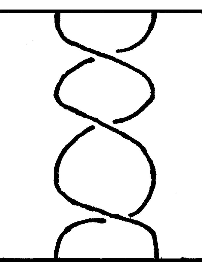
Figure 1: String solution with $n=2$, $k=1$ and schematic two-braid representation of the trefoil knot.

2.1 N=1 case

We start with the simplest case and take into consideration only one-component solution (13). Then equation (24) takes the form

$$R^{2}+2c_{0}R\cos[kz+n\phi]+c_{0}^{2}=0$$ (25)

and can be easily solved. We obtain that the defects are located in

$$R(\rho_{0})=c_{0},\;\;\;kz+n\phi=\pi+2\pi l,$$ (26)

where $l=0,1..n-1$. In other words, as we expected, our solutions appear to be strings located on a cylinder with a constant radius $\rho=\rho_{0}$. For any fixed $z=z_{0}$ the vector field winds $n$ times around the strings in the $z_{0}$ plane. Simultaneously, these $n$ strings wrap infinitely many times around the infinite long cylinder. There are $k$ coils on the interval $\Delta z=2\pi n$.
In Fig. 1 and Fig. 2 we present a part of two- and three-string solutions with $n=2,k=1$ and $n=3,k=\frac{2}{3}$ respectively. It is easy to observe that, after identification of the bases of the cylinder (i.e. upper and lower ends of the strings), both configurations can be associated with the trefoil knot. One can apply this procedure to other multi-string configurations and find various topologically inequivalent knots. This fact can be understood from the knot theory point of view. Indeed, it is a well-known result from knot and braid theory that every torus knot has a representation in terms of a braid diagram, obtained by the action of the braiding operators on a trivial braid.

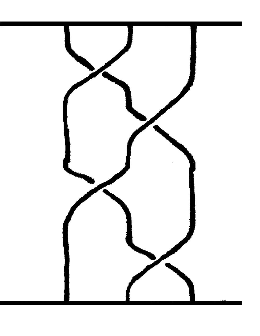
Figure 2: String solution with $k=2/3$, $n=2$ and schematic three-braid representation of the trefoil knot.

Moreover, the observation that all string configurations are located on a cylinder with constant radius is equivalent to the fact that the corresponding knots are torus knots. For example, one can see that our string solutions do not allow us to represent the figure-eight knot (fig. 3).

2.2 N=2 case

The second simple but interesting case we will investigate, is the case with two-component solution (13) and with $c_{0}=0$. Now one gets

$$2R_{1}^{2}R_{2}^{2}\cos[(k_{1}-k_{2})z+(n_{1}-n_{2})\phi]+R_{1}^{2}+R_{2}^{2}=0.$$ (27)

Then there is a central string located at the origin

$$\rho=0$$ (28)

as well as $n_{1}-n_{2}$ satellite strings

$$R_{1}(\rho_{0})=R_{2}(\rho_{0}),\;\;\;(k_{1}-k_{2})z+(n_{1}-n_{2})\phi=\pi,+2\pi l$$ (29)

$l=0,1..n_{1}-n_{2}$ which lie on the cylinder with a constant radius $\rho_{0}$. It can be checked that winding number of the central string is $Q_{c}=\mbox{min}\{n_{1},n_{2}\}$ whereas each of the satellite strings carries the unit topological charge.

2.3 Elliptic configurations

Now, we demonstrate how one can construct a solution describing strings located on an arbitrary surface topologically equivalent to cylinder. For example, we adopt before obtained solutions in the case of the cylindrically-elliptic coordinates $(\eta,\phi,z)$, where

$$x=\frac{1}{2}a\cos\phi\cosh\eta,$$

$$y=\frac{1}{2}a\sin\phi\sinh\eta,$$

$$z=z.$$ (30)

Then the eikonal equation possesses the following solutions

$$u(\eta,\phi,z)=Ce^{\pm ikz}e^{\pm i\sqrt{\lambda^{2}+\frac{k^{2}a^{2}}{4}}E\left(i\eta,1-\frac{4\lambda^{2}}{4\lambda^{2}+k^{2}a^{2}}\right)}e^{\pm i\sqrt{\lambda^{2}+\frac{k^{2}a^{2}}{4}}E\left(\phi,1-\frac{4\lambda^{2}}{4\lambda^{2}+k^{2}a^{2}}\right)}+c_{0},$$ (31)

where $E$ is elliptic integral the second kind. In order to guarantee uniqueness of the solution, parameters $\lambda$ and $k$ must fulfill relation

$$\frac{2}{\pi}\sqrt{\lambda^{2}+\frac{k^{2}a^{2}}{4}}E\left(1-\frac{4\lambda^{2}}{4\lambda^{2}+k^{2}a^{2}}\right)=n\in N.$$ (32)

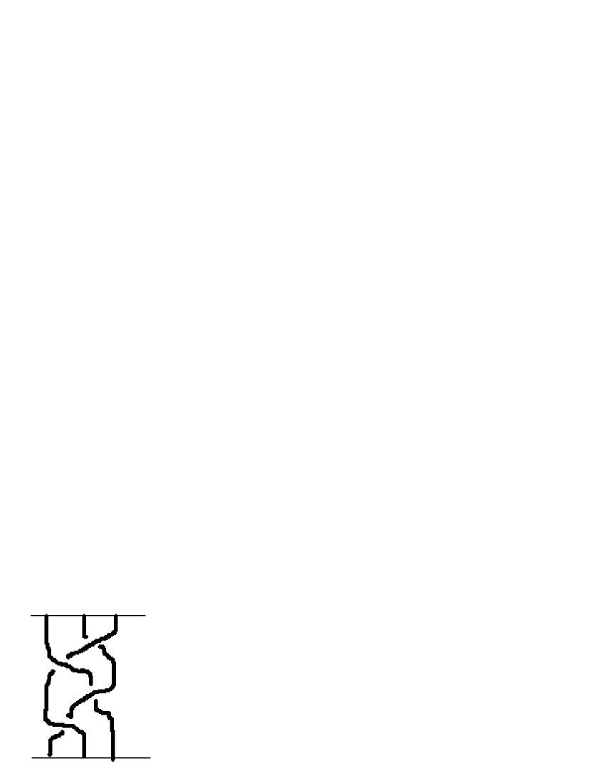
Figure 3: Three-braid representation of the figure-eight knot.

This new number $n$ fixes the topological contents of the configuration. We see that strings lie on a elliptic cylinder with a constant radius $\eta_{0}$

$$e^{\pm i\sqrt{\lambda^{2}+\frac{k^{2}a^{2}}{4}}E\left(i\eta_{0},1-\frac{4\lambda^{2}}{4\lambda^{2}+k^{2}a^{2}}\right)}=c_{0}$$ (33)

and are given by the formula

$$kz+\sqrt{\lambda^{2}+\frac{k^{2}a^{2}}{4}}E\left(\phi,1-\frac{4\lambda^{2}}{4\lambda^{2}+k^{2}a^{2}}\right)=\pi+2\pi l,$$ (34)

where $l=0,1..n-1$. The generalization to a configuration which describes strings located on any cylinder (or concentric cylinders) with an arbitrary shaped base is straightforward. One has to just introduce the pertinent coordinates and solve the eikonal equation.

It is also easy to notice that using the simplest topologically nontrivial solutions $u_{0}$ (12), (31) with $n=1$ we are able to obtain their multi-string generalizations (13). Let us for example consider cylindric string

$$u_{0}=C\frac{\rho e^{\sqrt{k^{2}\rho^{2}+1}}e^{i(\phi+kz)}}{1+\sqrt{k^{2}\rho^{2}+1}}.$$ (35)

We see that every solution in the form

$$u=F(u_{0}),$$ (36)

where $F$ is a real and differentiable function, also satisfies the eikonal equation. In particular, multi-string configurations are derived by taking $F$ as a polynomial function.

3 Topological Hedgehogs

In this section we take under consideration another type of topological objects with the non-trivial $\pi_{2}(S^{2})$ homotopy group i.e. hedgehogs or monopoles. The topology of these configurations emerges from the index of the map $\vec{n}_{\infty}:\;S^{2}\rightarrow S^{2}$.
Since the standard hedgehog possesses the rotational symmetry it is natural to apply the spherical coordinates $(r,\theta,\phi)$. The eikonal equation can be rewritten as

$$u^{\prime 2}_{r}+\frac{1}{r^{2}}u^{\prime 2}_{\theta}+\frac{1}{r^{2}\sin^{2}\theta}u^{\prime 2}_{\phi}=0.$$ (37)

Once again we use the separable variables method and assume the solution in the form

$$u=f(r)g(\theta)h(\phi).$$ (38)

Then equation (1) reads

$$\frac{f^{\prime 2}_{r}}{f^{2}}+\frac{1}{r^{2}}\left[\frac{g^{\prime 2}_{\theta}}{g^{2}}+\frac{1}{\sin^{2}\theta}\frac{h^{\prime 2}_{\phi}}{h^{2}}\right]=0.$$ (39)

In the standard manner we obtain that function $h(\phi)$ satisfies

$$\frac{h^{\prime 2}_{\phi}}{h^{2}}=-n^{2}$$ (40)

and have solutions

$$h(\phi)=Ae^{\pm in\phi},$$ (41)

where $n\in N$. Analogously the shape function is given by

$$\frac{f^{\prime 2}_{r}}{f^{2}}-\frac{m^{2}}{r^{2}}=0.$$ (42)

The pertinent solutions are

$$f(r)=Br^{\pm m},$$ (43)

here $m$ is any real number. Now, inserting equations (40) and (42) we are able to write down equation for the remaining angular variable

$$\frac{g^{\prime 2}_{\theta}}{g^{2}}-\frac{n^{2}}{\sin^{2}\theta}=m^{2}.$$ (44)

One can integrate it and find the following solutions

$$g(\theta)=C\left(\frac{\sqrt{n^{2}+m^{2}\sin^{2}\theta}-|m|\cos\theta}{\sqrt{n^{2}+m^{2}\sin^{2}\theta}+|m|\cos\theta}\right)^{\pm\frac{|n|}{2}}e^{\mp|m|\arctan\sqrt{\frac{n^{2}}{m^{2}}+\tan^{2}\theta}},$$ (45)

parameterize by two, previously introduced numbers $n,m$. Thus, the general solution of the eikonal equation in the spherical coordinates reads

$$u(r,\theta,\phi)=$$

$$Ar^{\pm m}\left(\frac{\sqrt{n^{2}+m^{2}\sin^{2}\theta}-|m|\cos\theta}{\sqrt{n^{2}+m^{2}\sin^{2}\theta}+|m|\cos\theta}\right)^{\pm\frac{|n|}{2}}e^{\mp|m|\arctan\sqrt{\frac{n^{2}}{m^{2}}+\tan^{2}\theta}}e^{\pm in\phi}.$$ (46)

Because of the fact that we are mainly interested in finding of solutions describing topological hedgehogs the following map must possess non-zero topological index

$$\vec{n}\;:\;S^{2}_{(r=\infty,\theta,\phi)}\rightarrow S^{2}_{|\vec{n}|=1}.$$ (47)

In other words, behavior of the unit vector field at the spatial infinity cannot be trivial. For example all configurations with $\vec{n}_{\infty}=\overrightarrow{\mbox{const}}.$ are, from our point of view, uninteresting since they lead to vanishing topological charge. It results in the fact that any configuration with the non-zero topological index shoul have $m=0$ in (43). Then the function $g$ can be rewritten in simpler form

$$g(\theta)=C\left(\tan\frac{\theta}{2}\right)^{\pm|n|}.$$ (48)

Thus, the general hedgehog configuration takes the form

$$u(\phi,\theta)=Ce^{\pm in\phi}\left(\tan\frac{\theta}{2}\right)^{\pm|n|}+c.$$ (49)

Identically as in the string case this solution can be generalized to a collection of the hedgehogs

$$u(\phi,\theta)=\sum_{j=1}^{N}Ce^{\pm in_{j}\phi}\left(\tan\frac{\theta}{2}\right)^{\pm|n_{j}|}+c,$$ (50)

where $N=1,2..$. One can check that the total topological charge, which tells us how many times the sphere $S^{2}_{(r=\infty,\theta,\phi)}$ is winded on the sphere $S^{2}_{|\vec{n}|=1}$, is given by the expression

$$Q=\mbox{max}\{n_{j},j=1..N\}.$$ (51)

Let us now notice that obtained eikonal hedgehog configurations (50) can be derived also from a dynamical system i.e. from $O(3)$ invariant action in the $(3+1)$ dimensional space-time

$$S=\int d^{4}x\frac{1}{2}(\partial_{\mu}\vec{n})^{2}.$$ (52)

After expressing the Lagrangian in terms of the complex scalar field $u$ we find that

$$L=\frac{2}{(1+|u|^{2})^{2}}\partial_{\mu}u\partial^{\mu}u^{*}.$$ (53)

Then the pertinent equation of motion reads

$$\frac{\partial_{\mu}\partial^{\mu}u}{(1+|u|^{2})^{2}}-2(\partial_{\nu}u)^{2}\frac{u^{*}}{(1+|u|^{2})^{3}}=0.$$ (54)

One can check that our configurations (50) fulfill this equation. It is due to the fact that they solve not only the eikonal equation but also the Laplace equation

$$\nabla^{2}u=0.$$ (55)

It should be underline that it is unlikely the string solutions found in the previous section. In this case no action, from which strings might be obtained as solutions of the pertinent field equations, is known.

4 Conclusions

In the present work two kinds of the static topological defects (strings and hedgehogs) living in three dimensional space have been discussed. These structures have been investigated by means of the complex eikonal equation.
In particular, many braided multi-string configurations have been found. Such multi-string solutions possess well defined topological charge fixed by the biggest value of the $n_{i}$ parameter in Ansatz (13), which is nothing else but the winding number of the vector field around the strings. All solutions have been presented in the analytical form. The most important feature of our strings is that they lie on a cylinder with a constant radius. Since every knot (knotted closed string) possesses its representation in terms of a braid (knots appear when we cut off a finite cylinder and identify its bases) we see that only torus knots (i.e. knots which can be plotted on a torus) can be constructed. In fact, it was observed in our recent paper. At this stage it is hard to justify whether problem of deriving of non-cylindrical strings and non-toroidal knots in the framework of the eikonal equation is only an artefact of the applied method (and such solutions should be found), or due to some yet unknown reasons these solutions are forbidden here. Unfortunately, it is still an open problem.
On the other hand an important problem associated with a property of the eikonal knots has been successfully solved. Namely, it has been proved that the eikonal strings (and in consequence eikonal knots as well) can be located on any surface topologically equivalent to a cylinder i.e. a tube with the base given by any reasonable closed curve, for instance ellipse.
This fact seems to be very important in the context of the Faddeev-Niemi effective action for the low energy gluodynamics where particles (glueballs) are described as knotted flux-tubes of the gauge field. As we discussed it before the properties of the eikonal knots appear to be quite similar to the properties of the Faddeev-Niemi hopfions. In particular, the eikonal knots serve as approximated solutions of the Faddeev-Niemi model. Thus, the results of our paper might find a physical application if we use obtained here elliptic string solutions (or other strings located on a’deformed’ cylinder)) and try to construct some new approximated solutions of the Faddeev-Niemi model.
As we said it before, the problem of the existence of the non-torus knots is still unsolved. However, there are some hints indicating that only torus knots can appear in the Faddeev-Niemi model [25]. Moreover, no non-torus knot has been observed using numerical methods [13], [14]. Undoubtedly, solving the problem of the existence of non-cylindrical open strings (or equivalently, non-toroidal closed strings) in the eikonal equation, we could shed any light on the appearance (or not) of such structures in the Faddeev-Niemi model. This issue requires farther studies.

This work is partially supported by Foundation for Polish Science FNP and ESF ”COSLAB” program.

References

- [1] O. Alvarez, L. A. Ferreira, J. Sánchez Guillén, Nucl. Phys. B 529, 689 (1998); L. A. Ferreira, E. E. Leite Nucl. Phys. B 547, 471 (1999).
- [2] L. A. Ferreira, J. Sánchez Guillén, Phys. Lett. B 504, 195 (2001).
- [3] C. Adam and J. Sánchez-Guillén, J. Math. Phys. 44, 5243 (2003); C. Adam, J. Sanchez-Guillen, hep-th/0412028.
- [4] K. Fujii, T. Suzuki, Lett in Math. Phys. 46, 49 (1998); K. Fujii, Y. Homma, T. Suziki, Phys. Lett. B 438, 290 (1998).
- [5] H. Aratyn, L. A. Ferreira and A. H. Zimerman, Phys. Lett. B 456, 162 (1999).
- [6] D. A. Nicole, J. Phys. G 4, 1363 (1978).
- [7] L. Faddeev, A. Niemi, Nature 387, 58 (1997); L. Faddeev, A. Niemi, Phys. Rev. Lett. 82, 1624 (1999); E. Langmann, A. Niemi, Phys. Lett. B 463, 252 (1999).
- [8] Y. M. Cho, Phys. Rev.D 21, 1080 (1980); Y. M. Cho, Phys. Rev. D 23, 2415 (1981); Y. M. Cho, Phys. Rev. Lett. 46, 302 (1981).
- [9] S. V. Shabanov, Phys. Lett. B 463, 263 (1999); S. V. Shabanov, Phys. Lett. B 458, 322 (1999);
- [10] Y.M. Cho, H.W. Lee, D.G. Pak, Phys. Lett. B 525, 347 (2002); B.A. Fayzullaev, M.M. Musakhanov, D.G. Pak, M. Siddikov, hep-th/0412282.
- [11] A. Niemi, hep-th/0312133; L. Faddeev, A. Niemi, U. Wiedner, Phys. Rev. D 70, 114033 (2004).
- [12] J. Gladikowski, M. Hellmund, Phys. Rev. D 56, 5194 (1997).
- [13] R. A. Battye and P. M. Sutcliffe, Phys. Rev. Lett. 81, 4798 (1998); R. A. Battye and P. M. Sutcliffe, Proc.Roy.Soc.Lond. A 455, 4305 (1999).
- [14] J. Hietarinta and P. Salo, Phys. Lett. B 451, 60 (1999); J. Hietarinta and P. Salo, Phys. Rev. D 62, 81701 (2000).
- [15] L. D. Faddeev, in 40 Years in Mathematical Physics, World Scientific, Singapore (1995); L. H. Kauffman, Knots and Physics, River Ridge, World Scientific, Hew York (2000); R. Dilao, R. Schiappa Phys. Lett. B 404, 57 (1997); R. Schiappa, R. Dilao, Phys. Lett. B 427, 26 (1998); E. Babaev, L. Faddeev, A. Niemi, Phys. Rev. B 65, 100512 (2002).
- [16] A. MacArthur, in Knots and Application, edited by L. H. Kauffman, World Scientific, Singapore (1995).
- [17] D. W. Sumners, Notices A. M. S. 42, 528 (1995).
- [18] A. Wereszczyński, Eur. Phys. J. C. in press, [hep-th/0410148]; ”Approximated Analytical Solution of the Faddeev-Niemi Model” in Proceedings of the conference ”Quark Confinement and the Hadron Spectrum VI”, edit. N. Brambilla et. all , AIP Conference Proceedings Series 756 (2005) 293.
- [19] C. Adam, J. Math. Phys. 45, 4017 (2004).
- [20] H. Aratyn, L. A. Ferreira and A. H. Zimerman, Phys. Rev. Lett. 83, 1723 (1999).
- [21] A. Wereszczyński, Eur. Phys. J. C 38 (2004) 261 [hep-th/0405155]; Mod. Phys. Lett. A 19 (2004) 2569 [math-ph/0405054]; Acta Phys. Pol. B 35 (2004) 2367 [math-ph/0410031]; Eur. Phys. J. C 41 (2005) 265 [math-ph/0504008].
- [22] L. A. Ferreira, hep-th/0406227.
- [23] A. E. Kudryavtsev, B. M. A. G. Piette, W. J. Zakrzewski, Nonlinearity 11, 783 (1998); T. I. Ioannidou, V. B. Kopeliovich, W. J. Zakrzewski, JHEP 95, 572 (2002).
- [24] T. Weidig, Nonlinearity 12, 1489 (1999); V. B. Kopeliovich, B. E. Stern, JETP Lett. 45, 203 (1987); J. R. Wen, T. Huang, BIHEP-TH-87-8 (1987).
- [25] T. R. Govindarajan, hep-th/9811171.