Anharmonic oscillator and double-well potential: approximating eigenfunctions

Abstract

A simple uniform approximation of the logarithmic derivative of the ground state eigenfunction for both the quantum-mechanical anharmonic oscillator and the double-well potential given by $V=m^{2}x^{2}+gx^{4}$ at arbitrary $g\geq 0$ for $m^{2}>0$ and $m^{2}<0$, respectively, is presented. It is shown that if this approximation is taken as unperturbed problem it leads to an extremely fast convergent perturbation theory.

Invited contribution to Letters in Mathematical Physics
to a Special Issue in memory of Professor Felix A. Berezin

For the last fifty years the quantum one-dimensional anharmonic oscillator $(m^{2}\geq 0)$ as well as the double-well potential problem $(m^{2}<0)$ described by the Hamiltonian

$${\cal H}\ =\ -\frac{d^{2}}{dx^{2}}\ +\ m^{2}x^{2}+gx^{4}\ ,$$ (1)

permanently attracted a lot of attention. The interest to these problems ranges from various branches of physics to chemistry and biology. It can not be an exaggeration to say that after the seminal papers by C. Bender-T.T. Wu at 1969-1973 BW in near thousand of physics articles the problem (1) was touched in one way or another. This seemingly simple problem revealed extremely rich internal structure which looks intrinsic for any non-trivial problem of quantum mechanics and even for quantum field theory. In particular, the obvious failure of the perturbation theory in powers of $g$ due to its asymptotic (divergent) nature in (1) pushed the development of non-perturbative methods. In practice, the anharmonic oscillator (1) served always as a test-ground for non-perturbative methods. Another important feature of the anharmonic oscillator (1) is related to the fact that it can be interpreted as one-dimensional quantum field theory $g\phi^{4}$ with zero spacial dimension, $(1,0)$. Hence, a study of (1) can be insightful to a realistic four-dimensional quantum field theory $g\phi^{4}$. The present article is devoted to the construction of a uniform approximation of the ground state eigenfunction of (1) in $x$-space which would continue to be valid for different values of the coupling constant $g$ and the parameter $m^{2}$. If such an approximation is constructed the energy of the ground state as well as different average values can be calculated with a guaranteed accuracy. We are not aware of previous attempts to construct a uniform approximation of the eigenfunctions.

Take the Schroedinger equation for (1)

$$-\frac{d^{2}\Psi}{dx^{2}}\ +\ m^{2}x^{2}\Psi\ +\ gx^{4}\Psi\ =\ E(m^{2},g)\Psi\quad,\quad\int_{-\infty}^{+\infty}|\Psi|^{2}dx<\infty\ .$$ (2)

For $m^{2}\geq 0$ the potential in (2) is a single-well potential, which describes the celebrated quartic anharmonic oscillator. For $m^{2}<0$ the potential in (2) is a two-well potential. It describes another celebrated potential - the so-called double-well potential (also known as the Higgs potential, Lifschitz potential). It is easy to check that for the energy in (2) the Symanzik scaling relation holds

$$E(m^{2},g)=g^{1/3}E\bigg{(}\frac{m^{2}}{g^{2/3}},1\bigg{)}\ ,\ \Psi(x;m^{2},g)=\Psi\bigg{(}xg^{1/6};\frac{m^{2}}{g^{2/3}},1\bigg{)}\ .$$

This manifests that the original problem (2) is essentially a single-parametric problem.

Eigenfunctions of (2) are sharply changing functions in $x$ being characterized by a power-like behavior at $|x|\rightarrow 0$ and an exponentially-decaying one at $|x|\rightarrow\infty$. In order to make them smooth we introduce the exponential representation for eigenfunctions

$$\Psi(x)\ =\ e^{-\varphi(x)}\ .$$ (3)

Following the oscillation (Sturm) theorem the function $\varphi$ should have logarithmic singularities at real $x$ which correspond to nodes of the wavefunction. Its regular part which appears after subtraction of those singularities should be slow-changing function of the power-like behavior at both small and large distances. After substitution of (3) into (2) we get a Riccati equation

$$y^{\prime}-y^{2}\ =\ E-\ m^{2}x^{2}\ -\ gx^{4}\ ,\quad y\ =\ \varphi^{\prime}\ =\ (\log\Psi(x))^{\prime}\ ,\ y(0)=0\ .$$ (4)

This famous equation serves as a basis for developing the WKB approximation scheme. Due to symmetric nature of the r.h.s. of (4) $x\rightarrow-x$ the function $y$ is odd. Its structure for the $n$th excited state should be

$$y\ =\ -\sum_{i=1}^{n}\frac{1}{x-x_{i}}\ +\ y_{reg}(x)\ ,$$ (5)

where $x_{i}$ is the position of $i$th node. The regular part $y_{reg}(x)$ should be a non-singular at real $x$ odd function which vanish at $x=x_{i},\ i=1,2,\ldots n$. It is evident that all non-zero $x_{i}$ come in pairs: once we have a node at $x=x_{i}$ always there exists a node at $x=-x_{i}$.

Now we consider the case of the ground state. According to above, in the phase (5) $n=0$ and singular part of $y$ is absent, $y=y_{reg}$. Hence, the function $y$ has no singularities at real $x$. It is easy to find its asymptotic behavior

$$y=g^{1/2}x|x|+\frac{m^{2}}{2g^{1/2}}\frac{|x|}{x}+\frac{1}{x}-\frac{4gE+m^{4}}{8g^{3/2}}\frac{1}{x|x|}-\frac{m^{2}}{2g}\frac{1}{x^{3}}+\ldots\quad\mbox{at}\ |x|\rightarrow\infty\ ,$$ (6)

while

$$y\ =\ Ex+\frac{E^{2}-m^{2}}{3}x^{3}+\frac{2E(E^{2}-m^{2})-3g}{15}x^{5}+\ldots\quad\mbox{at}\ |x|\rightarrow 0\ .$$ (7)

One can demonstrate that for any excited state the regular part $y_{reg}$ has similar formal expansions at $|x|\rightarrow 0,\infty$.

Let us develop a certain iterative procedure (perturbation theory) for solving the Riccati equation (4). From the point of finding the wave function it will be a multiplicative perturbation theory unlike a standard additive perturbation theory. Such a perturbation theory was developed for the first time by Price Price and then it was rediscovered many times. Eventually, it was called the ‘Logarithmic Perturbation Theory’ (for the history remarks and discussion see Turbiner:1984 and references therein).

As a first step we choose some square-integrable function $\Psi_{0}$ and calculate its logarithmic derivative

$$y_{0}=(\log\Psi_{0})^{\prime}=\frac{\Psi_{0}^{\prime}}{\Psi_{0}}\ .$$ (8)

It is clear that $\Psi_{0}$ is the exact eigenfunction of the Schroedinger operator with a potential

$$V_{0}=\frac{\Psi_{0}^{\prime\prime}}{\Psi_{0}}=y_{0}^{2}-y_{0}^{\prime}\ ,$$ (9)

where without a loss of generality we put their eigenvalue equals to zero, $E_{0}=0$. It is nothing but a choice of the reference point for eigenvalues. Now we can construct a perturbation theory for Riccati equation taking $\Psi_{0}$ and $y_{0},V_{0}$ as zero approximation, which characterizes the unperturbed problem. One can write the original potential $V=m^{2}x^{2}+gx^{4}$ as a sum,

$$V=V_{0}+(V-V_{0})\ \equiv\ V_{0}+V_{1}\ ,$$ (10)

thus, taking a deviation of the original potential from the potential of the zero approximation as a perturbation. We always can insert a formal parameter $\lambda$ in front of $V_{1}$ and develop a perturbation theory in powers of $\lambda$,

$$E=\sum_{k=0}^{\infty}\lambda^{k}E_{k}\quad,\quad y=\sum_{k=0}^{\infty}\lambda^{k}y_{k}\ ,$$ (11)

putting $\lambda=1$ afterwards. Perhaps, it is worth emphasizing that in spite of the fact that we study iteratively the equation (4), in general, this perturbation series has nothing to do with a standard WKB expansion. By substituting (11) into (4) we arrive at the equations which defines iteratively the corrections

$${y}_{k}^{\prime}-2y_{0}y_{k}=E_{k}-Q_{k}\ ,$$ (12)

where

$$Q_{1} = V_{1}\ ,$$

$$Q_{k} = -\sum_{i=1}^{k-1}y_{i}\cdot y_{k-i}\ ,\quad k=2,3,\ldots$$

It is interesting that the operator in the l.h.s. of (12) does not depend on $k$, while $Q_{k}$ in the r.h.s. can be interpreted as a perturbation on the level $k$. The solution of (12) can be found explicitly and is given by

$$E_{k} = \frac{\int_{-\infty}^{\infty}Q_{k}\Psi_{0}^{2}\,dx}{\int_{-\infty}^{\infty}\Psi_{0}^{2}\,dx}\ ,$$ (13)

$$y_{k} = \Psi_{0}^{-2}\int_{-\infty}^{x}(E_{k}-Q_{k})\Psi_{0}^{2}\,dx^{\prime}\ .$$ (14)

It is easy to demonstrate that

$$|y_{1}|\leq\mbox{Const}\ ,$$ (15)

provides a sufficient condition for this perturbation theory (11) to be convergent Turbiner:1984 . Note that this condition is very rough and can be strengthened.

The first two terms in the expansion of energy (11) in the above-described perturbation theory admit an interpretation in the framework of the variational calculus. Let us assume that our variational trial function $\Psi_{0}(x)$ is normalized to 1. We can calculate the potential $V_{0}$ where $\Psi_{0}(x)$ is the ground state eigenfunction and even put $E_{0}=0$ (see a discussion above). Pure formally, we construct the Hamiltonian $H_{0}=p^{2}+V_{0}$ for which $H_{0}\Psi_{0}(x)=0$. The variational energy is equal to

$$E_{var} = \int\psi_{0}H\psi_{0}=\underbrace{\int\psi_{0}H_{0}\,\psi_{0}}_{=E_{0}}+\underbrace{\int\psi_{0}\underbrace{(H-H_{0})}_{V-V_{0}}\psi_{0}}_{=E_{1}}$$ (16)

$$= E_{0}+E_{1}(V_{1}=V-V_{0})\geq E_{exact}\ .$$

Of course, $\Psi_{0}(x)$ could depend on free parameters. In this case both $V_{0}$ and $V_{1}$ depend on parameters as well. Minimization of $E_{var}$ with respect to the parameters can be performed and the variational principle guarantees that $E_{var}$ gives upper bound to the ground state energy. This simple interpretation (16) reveals a fundamental difference between perturbation theory and variational calculus. Variational estimates can be obtained independently on the fact that the perturbation theory associated with $\Psi_{0}(x)$ is convergent or divergent. However, it seems natural to remove this difference by requiring a convergence of the perturbation series. In this case by calculating the next terms $E_{2},E_{3},\ldots$ in (11) one can estimate the accuracy of variational calculation from one side and improve it iteratively from another side. An immediate criteria how to choose $\Psi_{0}(x)$ in order to get a convergent perturbation theory is to have the perturbation potential $V_{1}$ to be subordinate with respect to the non-vanishing potential of zero approximation $V_{0}$,

$$\Big{|}\frac{V_{1}}{V_{0}}\Big{|}<1\qquad,\qquad\mbox{for}\ |x|>R\quad.$$ (17)

This requirement has extremely non-trivial physical implication: in order to guarantee a convergence of perturbation theory a domain where the wavefunction is exponentially small should be reproduced as precise as possible. The same time a description of a domain where the wavefunction is of the order 1 is not important. It contradicts to a straightforward physics intuition and underlying idea of variational calculus which, in particular, requires a precise description of the domain where the wavefunction is of the order 1. Needless to say that namely the latter domain gives a dominant contribution to the integrals which define the energy in the variational calculations.

In our approach the main object for study is the logarithmic derivative of the wavefunction $y$ (see (4)). Since $y$ is antisymmetric, we will construct different interpolations of $y$ between $x=0$ and $x=\infty$ (see (6),(7)). In order to fulfil the requirement of the convergence (17) it is enough to take into account in these interpolations the leading term of the asymptotics at $|x|\rightarrow\infty$. Then the interpolation we have built is taken as zero approximation in our perturbation theory (11).

1. The simplest interpolation can be written as follows

$$y_{0}\ =\ ax+b\sqrt{g}x|x|\ ,$$ (18)

where $a,b$ are parameters. These parameters can be fixed either by taking them as variational and making a minimization of (16), $a_{min},b_{min}$, or following the idea to reproduce exactly the leading asymptotic behavior of $y$ at $x=\infty$ (see (6)), which requires to put $b=1$.

The ground state eigenfunction which corresponds to (18)

$$\psi_{0}^{(1)}=\exp\left\{-\frac{ax^{2}}{2}-b\frac{\sqrt{g}}{3}|x|^{3}\right\}\ ,$$ (19)

is the exact one for the potential

$$V_{0}=a^{2}x^{2}+b^{2}gx^{4}-2b\sqrt{g}|x|(1-ax^{2})\quad,\qquad E_{0}=a\ .$$

The perturbation potential $V_{1}=V-V_{0}$ is of the form

$$V_{1}=(m^{2}-a^{2})x^{2}+(1-b^{2})gx^{4}+2b\sqrt{g}|x|(1-ax^{2})\ ,$$

where the first two terms would disappear if we place $a=\pm m$, and $b=1$. In this case the first two terms in the perturbation theory are

$$E^{(1)}\equiv E_{0}+E_{1}=m+2\sqrt{g}\,\frac{\int_{0}^{\infty}x(1-mx^{2})e^{-mx^{2}-\frac{2\sqrt{g}}{3}x^{3}}dx}{\int_{0}^{\infty}e^{-mx^{2}-\frac{2\sqrt{g}}{3}x^{3}}dx}\ .$$ (20)

This expression leads to sufficiently high relative accuracy $\leq 10^{-2}$ (comparing to the accurate numerical results) for any $g\geq 0$ and value of $m^{2}$. It can be confirmed by calculation of the second correction $E_{2}$. However, a slight modification of of the interpolation (18) by including a term $1/x$, which is presented in (6), in a form

$$\tilde{\psi}_{0}^{(1)}\ =\ \frac{1}{\sqrt{1+cx^{2}}}\exp\left\{-\frac{ax^{2}}{2}-b\frac{\sqrt{g}}{3}|x|^{3}\right\}\ ,$$ (21)

where $c$ is a variational parameter, immediately leads to a drastic increase in accuracy (see Table 1). According to a quite simple, straightforward analysis of the second correction $E_{2}$ the variational energy deviates from exact one in $\lesssim 10^{-3}$ in relative units for both anharmonic oscillator and double-well potential for studied values of the parameters in (1) (see Table 1). When the second correction is taken into account the relative deviation reduces in two orders of magnitude becoming $\lesssim 10^{-5}$. It is worth mentioning that the quality of the approximation is reflected in the fact that $b_{min}$ deviates from the exact value $b=1$ in several percent.

	$g=2$		$g=1$		$g=2$
	$m^{2}=1$		$m^{2}=0$		$m^{2}=-1$
	$b=1$	$b_{min}$	$b=1$	$b_{min}$	$b=1$	$b_{min}$
		=1.09320		=1.13049		= 1.19610
$E^{(1)}$	1.6076526	1.6076150	1.0605130	1.0604314	1.0299142	1.0296682
$E_{2}$	-0.0001113	-0.0000735	-0.0001513	-0.0000692	-0.0003560	-0.0001070
$E^{(2)}$	1.6075413	1.6075415	1.0603617	1.0603622	1.0295581	1.0295612
Ref.Caswell:1979	1.60754130		1.06036209		1.02956085

Table 1: The Hamiltonian (1): Variational energy of the ground state and its corrections in perturbation theory (10-11) with $\tilde{\psi}_{0}^{(1)}$ (21) as input. The results are presented for two cases: when $b=1$ (the dominant term in asymptotics at $|x|\rightarrow\infty$ is reproduced exactly, see (6)) and when $b$ is taken as a variational parameter. In the latter the value of the second energy correction $E_{2}$ is reduced in two times.

The ground state function is symmetric w.r.t. $x\rightarrow-x$. Hence, it has an extremum at $x=0$. For any fixed $m^{2}<0$ there exists a value $g_{crit}$ such that for $g>g_{crit}$ this extremum is a maximum, otherwise a minimum. It is easy to find out that the critical point $g=g_{crit}$ corresponds to the vanishing ground state energy, $E=0$. Using the function (21) it was calculated the critical value $g_{crit}=0.302405$ for $m^{2}=-1$. It is quite interesting from physical point of view that for a family of double-well potentials with fixed $g$ there exists a domain $0>m^{2}>(m^{2})_{crit}$ where the ground-state eigenfunction has the maximum at the origin, which corresponds to the position of the unstable equilibrium similar to what takes place for the single-well case. For example, if $g=1$, the value of $(m^{2})_{crit}=-2.219597$. It implies that the particle in such a potential with the ground state energy above the barrier, $E>0$, somehow does not feel the existence of two minima.

2. The expression $E^{(1)}$ (20) reproduces the harmonic oscillator energy in the limit $g\to 0$. At $g=0$ the energy $E^{(1)}$ has a singularity as it must be. However, the expansion of (20) in powers of $g$ contains besides the integer powers in $g$ also half-integer powers which must not be present in the formal expansion of the energy in $g$ (see (11). Also the interpolation (18) reproduces the leading terms only in the expansions at $|x|\rightarrow 0,\infty$. It is a definite drawback of the interpolation (18) as well as (21) and it should be fixed. One of the simplest ways to fix it is to take the function

$$\psi_{0}^{(0,0)}\ =\ \frac{1}{\sqrt{1+c^{2}x^{2}}}\exp\left\{-\frac{A+ax^{2}/2+bgx^{4}/4}{(d^{2}+gx^{2})^{1/2}}\right\}\ ,$$ (22)

where $A,a,b,c,d$ are variational parameters. If the parameters are chosen to be

$$b=\frac{4}{3}\ ,\ a=\frac{d^{2}}{3}+m^{2}\ ,$$ (23)

the dominant and the first two subdominant terms in the asymptotic expansion (6) are reproduced by the function (22) exactly. In this case the convergency condition (15) is satisfied, the data for $|y_{1}|_{max}$ are in Table II. These two cases we call the Case 1 (two parameters are fixed (see (23)) to reproduce the growing terms in asymptotic expansion of $y$) and Case 2 (all five parameters in (22) are variational), respectively. Table II demonstrates that even the variational energy $E^{(1)}$ already provides extremely high accuracy: $10^{-8}-10^{-9}$ (Case 1) and $10^{-10}-10^{-11}$ (Case 2) for studied values of $m^{2},g$. These results reproduce (or exceed) the best known numerical results in literature. The order of the third energy correction $E_{3}$ is already in the three-four orders of magnitude less than the second correction $E_{2}$. It indicates to the extremely fast convergence of the series in the parameter $\lambda$ (see (11)). The energies $E^{(3)}(=E^{(1)}+E_{2}+E_{3})$ for given values of $m^{2},g$ are the most accurate among known in literature for the moment providing 16-17 significant digits (not all these digits are shown in Table II).

In the Case 1 we are focused to reproduce the behavior of the wavefunction at large distances while the behavior at small distances is defined as a result of the variational procedure. We can calculate the coefficient in front of $x$ in the logarithmic derivative of (22) which we denote $E_{exp}$ (see Table II). It should be the exact energy of the ground state in the case of the exact $y$ (see (7)). It is worth emphasizing that the deviation of $E_{exp}$ from $E^{(1)}$ (or from the exact energy $E$) appears in the fifth significant digit (!).

	$g=2$		$g=1$		$g=2$
	$m^{2}=1$		$m^{2}=0$		$m^{2}=-1$
$b$	$4/3$	$1.33813399$	$4/3$	$1.33361251$	$4/3$	$1.33190626$
$a=c^{2}/3+m^{2}$	1.79502293	–	0.37849775	–	1.10179879	–
$A$	0.7796	0.	0.2535	0.	-1.8484	-2.00747
$E^{(1)}$	1.607541303542	1.607541302751	1.060362094762	1.060362090514	1.029560850845	1.029560831475
$|y_{1}|_{max}$	0.0026	–	0.0029	–	0.0064	–
$E_{exp}$ (7)	1.607362918		1.059963236		1.030192509
$E_{2}$	-0.107E-08	-0.28E-09	-0.428E-08	-0.30E-10	-0.198E-07	-0.42E-09
$E^{(2)}$	1.607541302469	1.607541302469	1.060362090485	1.060362090484	1.029560831059	1.029560831054
$E_{3}$	-0.12E-12	-0.2E-13	-0.64E-12	0.1E-14	-0.47E-11	0.4E-13
$E^{(3)}$	1.607541302469	1.607541302469	1.060362090484	1.060362090484	1.029560831054	1.029560831054
Ref.Caswell:1979	1.607541303		1.06036209		1.029560848

Table 2: The Hamiltonian (1): Variational energy of the ground state and its corrections in perturbation theory (10-11) with $\psi_{0}^{(2)}$ (22) as input (the values of the corrections $E_{2,3}$ are rounded to very few first digits). For given $m^{2},g$ the first column corresponds to the parameters in $\psi_{0}^{(2)}$ which are chosen to reproduce exactly the first three terms in the asymptotic expansion (6), the second column all parameters are taken as variational. The energies with all accurate significant digits are framed.

The important question concerns to the deviation of the function (22) from the exact function. We consider the Case 1 when the growing asymptotics of $y$ at large distances is reproduced exactly. Due to this fact the perturbation theory for any studied $m^{2},g$ is fast convergent and $y_{1}$ is bounded for any real $x$,

$$|y_{1}|_{max}\sim 0.01\ .$$

Hence, the function (22) provides the uniform approximation of the exact $y$. In Fig.1 for $m^{2}=-1,g=2$ the behavior of $y_{0}$ it is shown while Fig.2 contains the behavior of the first correction $y_{1}$. It is worth mentioning that the maximal value of $y_{1}$: $|y_{1}|_{max}\sim 0.0029$ appears at $x\approx 3.9$ where the value of $\psi_{0}^{(0,0)}$ (22) is already extremely small, $\sim 10^{-9}$ and $y_{0}\sim 15.2$. Then $y_{1}\propto 1/x^{2}$ at $x\gg 1$. The ratio $y_{1}/y_{0}$ (see Fig.3) is the extremely small function which tends to zero at $|x|\rightarrow\infty$. A similar situation appears for other values of $m^{2},g$. For the double-well potential while approaching the semiclassical limit: $m^{2}\rightarrow-\infty$ and $g$ is kept fixed, e.g. $g=1$ - the accuracy provided by (22) remains unchanged: $E_{2}\lesssim-1.\times 10^{-6}$ for $m^{2}$ ranging from -1 to -30. In the same range the parameters of (22) are varied very little, being always of the same order of magnitude, although the value of the energy changes from $\sim 1$ to $\sim-105$. It was also calculated the parameters of the potential (1) which the ground state energy vanishes,

$$E(m^{2}=-2.2195970861,g=1)\ \approx\ 10^{-13}\ .$$

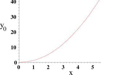
Figure 1: Logarithmic derivative $y_{0}$ of (22) as function of $x$

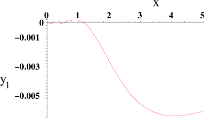
Figure 2: The first correction $y_{1}$ as function of $x$ for (22)

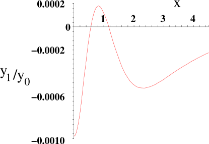
Figure 3: The ratio $y_{1}/y_{0}$ for (22)

It is worth mentioning that uniform approximation for eigenfunction of $(2k+p)$th excited state, $k=0,1,2,\ldots,p=0,1$ can be easily constructed as well. It has a form

$$\psi_{0}^{(k,p)}\ =\ \frac{x^{p}P_{k}(x^{2})}{\sqrt{1+c^{2}x^{2}}}\exp\left\{-\frac{A+ax^{2}/2+bgx^{4}/4}{(d^{2}+gx^{2})^{1/2}}\right\}\ ,$$ (24)

where $P_{k}$ is a polynomial of $k$th degree with positive roots. Parameters $a,b$ are always chosen following (23) in order to reproduce the growing terms in the asymptotic expansion of $y$ (Case 1 for the ground state)). In order to find the other parameters the orthogonality constraint should be imposed: for fixed $(k,p)$, (24) should be orthogonal to previously constructed functions $(m,p)$, at $m=0,1,2,\ldots,k-1$. It fixes some parameters in (24) while the remaining parameters are used as variational. It is worth mentioning that very important physical characteristic of (1) at $m^{2}<0$ is the energy gap between the energies of the ground state $(0,0$ and the first excited state $(0,1$ in the semiclassical limit: $m^{2}$ is kept fixed and $g\rightarrow\infty$. Although we do not provide concrete numerical results in this paper, this limit is reproduced with very high accuracy.

As a conclusion I would like to recollect my first and, in fact, the only scientific encounter with F.A. Berezin. It was in mid-1970s just before his breakthrough results in supermathematics. I was a recent graduate of Moscow Institute for Physics and Technology just hired by Institute for Theoretical and Experimental Physics. Among theoretical physicists F.A. Berezin had a reputation of the unique mathematician who was able to understand what physicists are talking about and with whom one could discuss your mathematical difficulties. He had run a weekly seminar at Mathematics Department of Moscow State University. By accident I went to one of his seminars but I could not say that I understood much. During the seminar break in the moment when I was ready to leave he approached to me, introduced himself and asked what I am working on. I answered that for already several years I had been trying desperately to find an analytic solution of the anharmonic oscillator $x^{4}$ (see (1)). Or, at least, to understand why all my attempts had failed. He immediately said: ”I know an anharmonic oscillator, which has an analytic solution! Take a function $e^{-x^{4}}$, differentiate it twice and divide the result by $e^{-x^{4}}$. This is the anharmonic oscillator potential where you know an exact eigenfunction.” Then we talked for several minutes. In the end, he said that together with M.A. Shubin (now a Distinguished Professor at Northeastern University in Boston) they would write a book on the Schroedinger equation and one day if I did not mind they could ask my opinion or advice. He introduced M.A. Shubin to me with whom I become a lifelong friend. After the seminar F.A. Berezin, M.A. Shubin and myself took a walk to the nearest metro station. I remember it was a very interesting conversation about mathematics but I do not remember what it was about - I was engrossed with thinking about the remarks of F.A. Berezin.

This short meeting had struck me and influenced strongly my scientific life. From human point of view I was deeply impressed how serious and friendly he was towards me, almost still a student. After some time I understood that instead of solving the Schroedinger equation with an already given potential one can generate a zillion potentials for which a single eigenstate is known exactly. It led me to an idea of choosing one of such potentials as a zero approximation to construct a convergent iterative procedure for a given eigenstate, not for the whole spectra Turbiner:1979 . Another idea was related to a natural question of how to construct a potential for which not one but two or more eigenstates can be found explicitly. It led to a discovery of quasi-exactly-solvable quantal problems Turbiner:1988 . A few years after our meeting F.A. Berezin tragically died and the chance to discuss with him disappeared, but all my life I keep a memory of him. Recently, I told this story to one of the greatest minds in today’s mathematics who was among very close colleagues and friends of F.A. Berezin. He responded with sorrow that ”… only after his death we realized how strong was his influence on all of us and, eventually, how great he was!”

Acknowledgments

Author thanks J.C. Lopez Vieyra the interest to the work and a help with computer calculations. The work is supported in part by DGAPA grant No.IN124202 (Mexico).

References

- (1) C.M. Bender, T.T. Wu, ‘Anharmonic Oscillator’, Phys. Rev. 184, 1231 (1969); ‘Anharmonic Oscillator.II’, Phys. Rev. D 7 , 1620 (1973)
- (2) P.J. Price, Proc. Phys. Soc. London 67, 383 (1954)
-
(3)
A.V. Turbiner, ‘The Problem of Spectra in Quantum Mechanics and the
‘Non-Linearization’
Procedure’,
Usp. Fiz. Nauk. 144, 35-78 (1984),
Sov. Phys. - Uspekhi 27, 668-694 (1984) (English Translation) -
(4)
W.E. Caswell, ‘Accurate energy levels for the anharmonic
oscillator and a summable series for the double-well
potential in perturbation theory’,
Ann.Phys. 123, 153-184 (1979) -
(5)
A.V. Turbiner,
‘A New Approach to Finding Levels of Energy of Bound States
in Quantum Mechanics: Convergent Perturbation Theory’,
Soviet Phys. – Pisma ZhETF 30, 379-383 (1979).
JETP Lett. 30, 352-355 (1979) (English Translation) -
(6)
A.V. Turbiner,
‘Spectral Riemannian Surfaces of the Sturm-Liouvile
Operator and
Quasi-Exactly-Solvable Problems’,
Funktsional’nyi Analiz i eqo Prilozhenia 22, 92-94 (1988),
Soviet Math. – Functional Anal. and its Appl. 22, 163-166 (1988)
(English Translation);
‘Quantum Mechanics: the Problems Lying between Exactly-Solvable and Non-Solvable’,
Soviet Phys. - ZhETF 94, 33-45 (1988),
JETP 67, 230-236 (1988) (English Translation);
‘Quasi-Exactly-Solvable Problems and the Group’,
Comm.Math.Phys. 118, 467-474 (1988)