Evolving Networks and Birth-and-Death Processes

Abstract

Using a simple model with link removals as well as link additions, we show that an evolving network is scale free with a degree exponent in the range of $(2,4]$. We then establish a relation between the network evolution and a set of non-homogeneous birth-and-death processes, and, with which, we capture the process by which the network connectivity evolves. We develop an effective algorithm to compute the network degree distribution accurately. Comparing analytical and numerical results with simulation, we identify some interesting network properties and verify the effectiveness of our method.

Growing Networks and Pure Birth Processes

The first growing network model, i.e., the BA model proposed by Albert, Baraba$\acute{a}$si, Jeong Barabasi99a , predicts a power-law network degree distribution with exponent $\gamma=3$, whereas the degree exponents of many real complex networks are found empirically in the range of $(2,4)$ Newman03 ; Albert . This has motivated extensive research to modify the basic BA model to match with practical scale-free networks. These variations can be summarized by the following general BA model:

(i) Initialization: $n_{0}$ nodes are given at time $t=0$;

(ii) Growth: at the $t$th time step, a new node and $m(t)(\leq t+n_{0})$ new links from this node are added;

(iii) Preferential attachment: the new node is connected to an existing node $i$ according to the following probability $\Pi(k_{i})=f(k_{i})/\sum_{j}f(k_{j})$, where $k_{i}$ is the number of degrees of node $i$ and $f(k_{i})$ is pre-selected function.

With general $m(t)$ and $f(k_{i})$, this model is analytically intractable and is very complicated for simulation study. We may simplify this model in two ways. Setting $m(t)=m$, i.e., the number of links in the network increase linearly, the growth of the network is stationary. Assuming $f(k_{i})=k_{i}$ further, we have the basic BA model. If we set $f(k_{i})=(1-p)k_{i}+p$ instead, where $p$ is the probability of randomly selecting an old node, the model reduces to Liu et al. Liu02 ’s model with $\gamma=3+p/[m(1-p)]$. In Bianconi and Barabsi Bianconi01 ’s fitness model, $f(k_{i})=\eta_{i}k_{i}$, where $\eta_{i}$ is chosen from a distribution $\rho(\eta)$. If $\rho(\eta)$ is uniform, $\gamma=2.255$. Alternatively, we can also first set $f(k_{i})=k_{i}$. With a time-dependent number of new links added at each time step, the growth of a network is non-stationary. For example, with the accelerating function $m(t)=mt^{\theta}$, $0\leq\theta<1$ proposed by Dorogovtseva and Mendes Dorogovtseva01 , the degree exponent $\gamma=(3-\theta)/(1-\theta)$ and the non-stationary exponent $z=2\theta/(1-\theta)$. Shi, Chen and Liu Shi04 proposed a slower accelerating function $m(t)=m\ln t$, $t\geq 2$.

Shi, Chen and Liu Shi04 established a relation between the connectively of a growing network and a set of non-homogeneous pure birth processes (PBP) and found numerically that $\gamma\approx 3.1$ and the non-stationary exponent is very small for the case of $m(t)=m\ln t$. It can be observed that the degree distribution curves of growing networks in Shi04 is snake like with a slightly downward bending head section as illustrated in figure 1 (see, also Shi04 for similar figures).

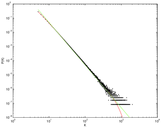
Figure 1: The degree distribution for the BA model with $m=5$, $S=3$ and $t=150000$: by the analytical method in solid green line; by simulation in dotted black line; and by the PBP method in solid red line.

There are other ways to extend the BA model. Readers can refer to Albert for a comprehensive review.

A Model of Evolving Networks and Dynamic Equation

Albert and Baraba$\acute{a}$si Ab considered a model of the evolving network in which some old links are rewired at each time step (see Section 4). We observe from many real networks that beside adding new nodes and links, some old nodes and links can also be removed as a network evolves. In other words, many networks display a dynamic evolving process. We propose the following simple model to capture the basic features of the above evolving network.

(i) Initialization: There are $n_{0}$ fully connected initial nodes.

(ii) Link removal: At each time step, $c$ old links are removed as follows. We first select node $i$ with the anti-preferential probability similar to that used in K02

$$\Pi^{*}(k_{i})=ak_{i}^{-1},$$ (1)

where $a$ is used as a normalized factor such that $a^{-1}=\sum_{i}k_{i}^{-1}$. We then choose node $j$ from the neighborhood of node $i$ (denoted by $O_{i}$ ) with probability $K_{i}^{-1}\Pi^{*}(k_{j})$, where $K_{i}=\sum_{j\in O_{i}}\Pi^{*}(k_{j})$. The link connecting nodes $i$ and $j$ is removed. We repeat this procedure $c$ times to remove $c$ existing links. Finally, isolated nodes are removed from the network.

(iii) Link addition: At each time step, a new node is added to the system and $m(\leq n_{0})$ new links from the new node are connected to $m$ different existing nodes. A node $i$ with degree $k_{i}$ will receive a connection from the new node with a Bayes’ preferential probability

$$\Pi(k_{i})=\frac{k_{i}+1}{\sum_{j}(k_{j}+1)}.$$ (2)

The above model is different from the existing ones in that it removes links instead of rewiring links. Furthermore, isolated nodes are removed in our model.

By the continuum theory, $k_{i}(t)$ approximately satisfies the following dynamic equation

$$\frac{\partial k_{i}}{\partial t} = m\Pi(k_{i})-c\left[\Pi^{*}(k_{i})+\sum_{j\in O_{i}}\Pi^{*}(k_{j})K_{j}^{-1}\Pi^{*}(k_{i})\right]$$ (3)

$$\approx m\frac{k_{i}+1}{[2(m-c)+1]t}-c\frac{2}{t},$$

where the last approximation is based on $\sum_{j}(k_{j}+1)=2(m-c)t+N(t-1)\approx[2(m-c)+1]t$, $\sum_{j\in O_{i}}K_{j}^{-1}\Pi^{*}(k_{j})\approx 1$, and, in the mean-field sense, $ak_{i}^{-1}\approx[N(t-1)]^{-1}\approx 1/t$, in which $N(t-1)$ is the number of non-isolated nodes at time step $t$.

Let $t_{i}$ be the time step when node $i$ is added to the network. Initially, node $i$ has $k_{i}(t_{i})=m$ links, thus the above equation has the following solution

$$x_{i}(t)=|k_{i}(t)+B-m|=B\left(\frac{t}{t_{i}}\right)^{\beta},$$ (4)

with the dynamic exponent

$$\beta=\beta(m,c)=\frac{m}{2(m-c)+1}$$ (5)

and the dynamic coefficient

$$B=B(m,c)=m+\frac{m-2c[2(m-c)+1]}{m}.$$ (6)

In the solution procedure, we require $0<\beta<1$ and $B>0$ for the solution to be feasible. Some simple analysis of the above formulas shows that $m>2c$ is a sufficient condition for equation (3) to have a feasible solution.

Assume that $t_{i}$ follows a uniform distribution over interval $(0,t)$. We have, by (4)

$$P(x)=\frac{1}{\beta}B^{1/\beta}x^{-\gamma},$$ (7)

where $x\in[B,\infty)$ following from (4) and the degree exponent

$$\gamma=1+\frac{1}{\beta}=3+\frac{1-2c}{m}.$$ (8)

Equation (8) shows that this system self-organizes into a scale-free network with $2<\gamma\leq 4$.

The next step is to obtain the network degree distribution. For $B\geq m$, we have, following the standard mean field approach Ab , the explicit solution of dynamic equation (3)

$$k_{i}(t)=B\left[\left(\frac{t}{t_{i}}\right)^{\beta}-1\right]+m$$ (9)

and the network degree distribution

$$P(k)=\frac{1}{\beta}B^{1/\beta}(k+B-m)^{-\gamma}.$$ (10)

For $B<m$, the continuum theory does not render an accurate solution, and we need a different method.

Birth-and-Death Processes of Network Connectively

The dynamics of the degree of a node in an evolving network is closely related to Markov processes. Let $K_{i}(t)$ be the degrees of node $i$ at time $t$. Since $K_{i}(t+1)$ only depends on $K_{i}(t)$ and allows the removal of old links for our model, $\{K_{i}(t),t=i,i+1,\ldots\}$ is a discrete-time Markov process with the state space $\Omega=\{0,1,2,\ldots\}$.

By (3), the probability that node $i$ with degree $k(\geq 1)$ is connected to a new node at time step $t$ is approximately $g_{t}(k)=(1-2c/t)m\Pi(k)\approx m\Pi(k)=m(k+1)/([2(m-c)+1]t)$. The probability that note $i$’s degree decreases by $1$ is approximately $(2c/t)\left[1-m\Pi(k_{i})\right]\approx 2c/t$, while the probability that its degree decreases by more than 1 is $o(t)$ and will be ignored. Thus, the probability that the degree of node $i$ remains the same is $h_{t}(k)=1-g_{t}(k)-2c/t$. This shows that $K_{i}(t)$ is in fact a non-homogeneous birth-and-death process (BDP). In addition, we set $p_{00}=1$ since we remove isolated nodes and $p_{kk}=1$ when $k>m+t-i$. In summary, for $t=i,i+1,i+2,\ldots$, the one-step transition probability matrix of node $i$ at time $t$ is given by

$$\textbf{P}_{i}(t+1)=\left[\matrix{1&0&&\cr&\cr 2c/t&h_{t}(1)&g_{t}(1)&&\cr\ddots&\ddots&\ddots&&\cr&\cr&2c/t&h_{t}(m+t-i)&g_{t}(m+t-i)&&\cr&\cr&&0&1&0&\cr&&\hskip 28.45274pt\ddots&\hskip 28.45274pt\ddots&\hskip 28.45274pt\ddots&}\right].$$ (11)

Denote $f_{i,n}(t)=P\{K_{i}(t)=n\}$ for $n=0,1,2,\ldots$ and $\vec{f}_{i}(t)=(f_{i,0}(t),f_{i,1}(t),\cdots,f_{i,n}(t),\cdots)$. Obviously, $\vec{f}_{i}(i)=(0,0,\cdots,0,1,0,\cdots)=\vec{e}_{m}$ where $e_{i,m}(i)=1$. By density evolution, the $(t+1)$th-step probability vector $\vec{f}_{i}(t+1)$ for node $i$ is given by

$$\vec{f}_{i}(t+1)=\vec{e}_{m}\cdot\textbf{P}_{i}(i+1)\cdot\textbf{P}_{i}(i+2)\cdots\textbf{P}_{i}(t+1),~{}~{}~{}~{}t=i,i+1,\ldots.$$ (12)

Let

$$\vec{F}^{(S,t)}(t+1)=\sum_{i=S}^{t}\vec{f}_{i}(t+1)=\sum_{i=S}^{t}\vec{e}_{m}\textbf{P}_{i}(i+1)\cdot\textbf{P}_{i}(i+2)\cdot\cdot\cdot\textbf{P}_{i}(t+1),$$ (13)

where the integer $S\geq 1$ is needed technically for the transition probability matrix. For the choice of $S$ and its impact on computation, please refer to Shi04 .

Generally, it would be extremely difficult to calculate (13). Fortunately, we can find the following relations:

$$\vec{e}_{m}\textbf{P}_{i}(t)=\vec{e}_{m}\textbf{P}_{S}(t),~{}~{}~{}~{}i=S+1,S+2,...;~{}~{}t=i+1,i+2,...;$$ (14)

and, in general, for $s=1,2,...~{}$

$$\vec{e}_{m}\textbf{P}_{i}(t)\textbf{P}_{i}(t+1)\cdot\cdot\cdot\textbf{P}_{i}(t+s)=\vec{e}_{m}\textbf{P}_{S}(t)\textbf{P}_{S}(t+1)\cdot\cdot\cdot\textbf{P}_{1}(t+s).$$ (15)

Thus we obtain the following key algorithm

$$\vec{F}^{(S,t)}(t+1)=((\cdot\cdot\cdot(\vec{e}_{m}\textbf{P}_{S}(S+1)+\vec{e}_{m})\textbf{P}_{S}(S+2)+\cdot\cdot\cdot)+\vec{e}_{m})\cdots\textbf{P}_{S}(t+1).$$ (16)

The right-hand side of (16) can be efficiently computed with a complexity of $O(t^{2})$ Shi04 .

The degree distribution of a network can be determined by the average of the degree distributions of all the nodes. Therefore, for a sufficiently large $t$, we have

$$P(k)\approx P(k,t+1)=\frac{F_{k}^{(S,t)}(t+1)}{t-S+1}.$$ (17)

As a bonus, we can also estimate the number of non-isolated nodes from (17) as follows

$$N(t)\approx(t+1)[1-P(0,t+1)],$$ (18)

noting that $P(0,t+1)$ is the probability that a node is isolated at time step $t+1$. This index cannot be obtained from (10).

We note that there are also inaccuracies in the transition probability matrices, and we can only perform a finite number of computation steps to estimate the asymptotic network behavior. To verify the BDP method, we compare the computation results with simulation.

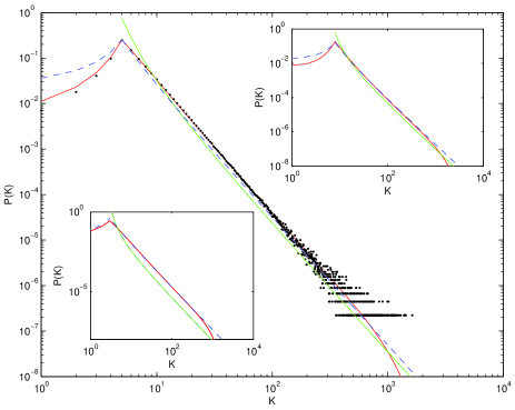
Figure 2: The degree distribution obtained by (10) in solid green line; by (19) in dash blue line; by simulation in dotted black line; and by the BDP method in solid red line for $m=5$, $c=1$, $S=4$ and $t=150000$. The settings for the inserts are the same as those of the main figure, except $m=3$ and $c=1$ for the bottom left insert and $m=8$ and $c=2$ for the top right insert, and no simulation results are given.

From figure 2, we see that the network degree distribution curves obtained by the BDP method and by simulation match very well. Our method predicts a horse head-like distribution curve, with its middle section displaying the expected scale-free state. Because we can only perform a finite number of computation steps, there is an inward bend at the tail of the distribution curve (see Shi04 for more detailed discussion). The degree exponent and coefficient can be estimated by applying the least square method to the data generated from $P(k)\in(10^{-4},10^{-6})$.

The numerical results from the birth-death processes clearly show that the network degree distribution curve has a very different head section. This motivates us to construct the following approximation for the degree distribution when $B<m$, noticing also from (4) that, when $B<m$, $x_{i}(t)$ achieves the minimum at $k_{i}(t)=m$ and is symmetric

$$P(k)\approx\left\{\begin{array}[]{ll}C\frac{1}{\beta}(k-\mu)^{-\gamma},{}&k\geq m\\ C\frac{1}{\beta}(2m-\mu-k)^{-\gamma},{}&k<m\end{array}\right.$$ (19)

where $\mu$ is a fitted parameter and the coefficient

$$C=(2m-\mu)^{\frac{1}{\beta}}/\left[2\left({\frac{2m-\mu}{m-\mu}}\right)^{\frac{1}{\beta}}-1\right]$$ (20)

is a normalizing constant such that $\int_{0}^{\infty}P(k)dk=1$.

Empirically, we find that when $\mu=0.2m+(c-1)$, the approximation (19) is very accurate for the overall distribution and captures the pattern of the small degree distribution, as shown in the small inserts in figure 2. The figures also show that (10) cannot provide probabilities for degrees smaller than $m$, and it visibly over estimates other small degree probabilities and under estimate large degree probabilities.

Application to the Albert-Barab$\acute{a}$si model

The model proposed by Albert Barab$\acute{a}$si Ab starts with $n_{0}$ isolated nodes, and performs one of the following operations at each time step:

(i) Add $m(\leq n_{0})$ new links with probability $p$: Select a node randomly as the starting point of the new link and then select the other end of the link with the preferential probability (2). Repeat this process $m$ times.

(ii) Rewire $m$ links with probability $q$: Select randomly a node $i$ and a link $l_{ij}$ connected to it. Remove this link and replace it with a new link $l_{ij^{\prime}}$ that connects $i$ to node $j^{\prime}$ which is chosen with the preferential probability (2). Repeat this process $m$ times.

(iii) Add one new node with probability $r=1-p-q$: The new node has $m$ new links that are connected to different existing nodes with the preferential probability (2).

By the continuum theory, Albert and Barab$\acute{a}$si obtained the following dynamic equation

$$\frac{\partial k_{i}}{\partial t}\approx m\frac{k_{i}+1}{[2m(1-q)+r]t}+m\frac{p-q}{rt},$$ (21)

and from which they derived the network degree distribution

$$P(k)=\frac{1}{\beta}(m+\tau)^{\frac{1}{\beta}}(k+\tau)^{-\gamma},$$ (22)

where $\tau=(p-q)(2m(1-q)/r+1)+1$ and the degree exponent

$$\gamma=1+\frac{1}{\beta}=3+\frac{r-2mq}{m}.$$ (23)

Obviously, (22) is valid only when $m+\tau>0$. Thus for the Albert-Baraba$\acute{a}$si model, the network degree distribution is scale-free only when parameters $p$ and $q$ satisfy

$$q<q_{max}=min\{1-p,(m+1-p)/(2m+1)\}.$$ (24)

Now, we use birth-and-death processes to discuss the Albert-Baraba$\acute{a}$si model. By (21), the one-step transition probability matrix of node $i$ at time $t$ is given by

$$\textbf{P}_{i}(t+1)=\left[\matrix{1-g_{t}(0)&g_{t}(0)&&\cr&\cr mq/rt&h_{t}(1)&g_{t}(1)&&\cr\ddots&\ddots&\ddots&&\cr&\cr&mq/rt&h_{t}(m+t-i)&g_{t}(m+t-i)&&\cr&\cr&&0&1&0&\cr&&\hskip 28.45274pt\ddots&\hskip 28.45274pt\ddots&\hskip 28.45274pt\ddots&}\right],$$ (25)

where $g_{t}(k)\approx(m(k+1)/([2m(1-q)+r]t))+mp/rt$ and $h_{t}(k)=1-g_{t}(k)-mq/rt$.

The results from (22) and the BDP method are compared in figures 3 and 4. The distribution curves of the two methods match very well in the middle section. Again, the distribution curves from the BDP method are horse head like with a downward bending head. (22) over estimates small degree probabilities and does not provide the probabilities for degrees smaller than $m$.

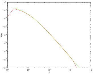
Figure 3: The degree distribution obtained by (22) in solid green line and by the BDP method in solid red line for $m=2$, $p=0.6$, $q=0.1$, $S=2$ and $t=100000$.

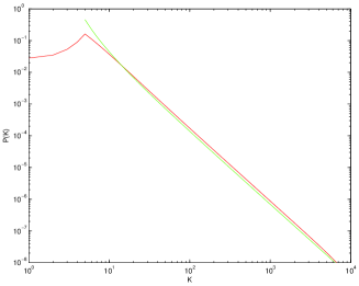
Figure 4: The degree distribution obtained by (22) in solid green line and by the BDP method in solid red line for $m=5$, $p=0.2$, $q=0.4$, $S=4$ and $t=150000$.

We summarize the results and findings in this paper as follows: (1) We introduce a simple yet flexible model of evolving networks with both addition and removal of links and nodes. The removal of both links and isolated nodes is new; (2) The connection between an evolving network and a set of non-homogenous birth-and-death processes provides an efficient algorithm to numerically calculate the network degree distribution. With this method, we reveal the complete process by which a network evolves into a scale-free state; (3) With the close match between the numerical results and simulation results, our birth-death method provides an efficient and reliable substitution to simulation, in particular since the existing analytical methods cannot handle more complicated network mechanisms and the computational requirements of simulation are often too high; (4) We find that the method based on the continuum theory is not suitable for small degree distribution and under estimates large degree probabilities; (5) The horse head-like degree distribution curves have been observed in a number of real networks, such as the actor collaborations and word co-occurrences networks (see figure 1 (d) and (e) in Newman Newman02 ). Using the birth-and-death process method, we demonstrate that the distribution curves of growing network are snake head like while the distribution curves of evolving networks are horse head like; and (6) Degree distributions of evolving networks have two distinct sections and the maximum probability occurs at degree $m$.

References

- (1) A.-L. Barabsi, R. Albert, H. Jeong, Physica A 272, 173 (1999).
- (2) M. E. Newman, SIAM Review 45, 167 (2002).
- (3) R. Albert and A.-L. Barabsi, Rev. Mod. Phys. 74, 47 (2002).
- (4) Z. Liu, Y. Lai, N. Ye, P. Dasgupta, Physics Letters A 303, 337 (2002).
- (5) G. Bianconi, A. Barabási, Phys. Rev. Lett. 86, 5632 (2001).
- (6) S.N. Dorogovtsev, J.F.F. Mendes, Phys. Rev. E 63, 025101 (2001).
- (7) D. Shi, Q. Chen, L. Liu, Phys. Rev. E 71, 036140 (2005).
- (8) R. Albert and A.-L. Barabsi, Phys. Rev. Lett. 85, 5234 (2000).
- (9) K. Klemm, V. M. Eguluz, Phys. Rev. E 65, 057102 (2002).
- (10) M. E. Newman, in Handbook of Graphs and Networks —- From the Genome to Internet, Bornholdt S. and Schuster H. G. (eds), Wiley-VCH, 35(2002).