A frequency domain model of multimode circular microresonators for filter applications in integrated optics is investigated. Analytical basis modes of 2D bent waveguides or curved interfaces are combined with modes of straight channels in a spatial coupled mode theory framework. Free of fitting parameters, the model allows to predict quite efficiently the spectral response of the microresonators. It turns out to be sufficient to take only a few dominant cavity modes into account. Comparisons of these simulations with computationally more expensive rigorous numerical calculations show a satisfactory agreement.

Introduction

Nowadays due to their superior selectivity, compactness, and possibility of dense integration, microresonators (MRs) become attractive for application as wavelength add/drop filters [1]. A typical microresonator setting, where a ring/disk shaped cavity is placed between two straight waveguides, is shown in Fig. 1. In this paper, we outline a spatial coupled mode theory (CMT) based model of 2D circular multimode optical microresonators.

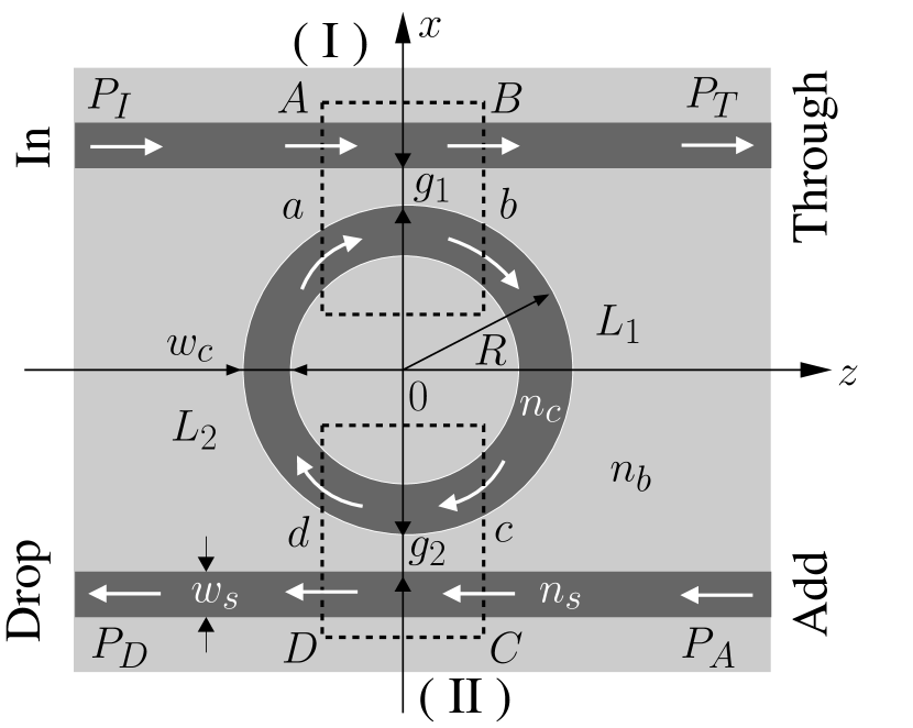
Figure 1: Functional decomposition of 2D microresonators: $R$ is the radius of the cavity with a core refractive index $n_{c}$ and a width $w_{c}$ ($=0$, for disks). The straight waveguides have a core refractive index $n_{s}$ and a width $w_{s}$; $g_{1}$ and $g_{2}$ are the separation distances between the cavity and the straight waveguides; $n_{b}$ is the background refractive index; $L_{1}$ and $L_{2}$ denote the lengths of the cavity segments which are not included in the coupler regions. The letters $A,B,C,D$ and $a,b,c,d$ denote the coupler port planes.

Abstract resonator model

For modeling purposes, the MR is decomposed into two bent-straight waveguide couplers, represented by the blocks (I) and (II), which are connected to each other by two segments of the cavity. The external connections are provided by straight waveguides. Here we consider only forward propagating modes of uniform polarization. We assume that all elements are linear and that the back reflections inside the couplers and the cavity are negligible. Outside the couplers, the interaction between the constituent waveguides is assumed to vanish. We consider a frequency domain description of the optical field. The vacuum wavelength $\lambda$ prescribes the real angular frequency $\omega$. Assume that $N_{s}$ modes of the straight waveguides and $N_{b}$ bend modes of the cavity are taken into account.

Let $\gamma^{p}$ be the complex propagation constant of the $p$’th cavity mode. The variables $A^{q},B^{q},C^{q},D^{q}$ and $a^{p},b^{p},c^{p},d^{p}$ denote the directional amplitudes of these properly normalized modes in the coupler port planes, combined into amplitude vectors $\mathbf{A},\mathbf{B},\mathbf{C},\mathbf{D}$ and $\mathbf{a},\mathbf{b},\mathbf{c},\mathbf{d}$. Let $\mbox{\sf S}^{\mbox{\scriptsize I}}$ and $\mbox{\sf S}^{\mbox{\scriptsize II}}$ be the scattering matrices for coupler I and II respectively, i.e.

$$\begin{bmatrix}\mathbf{b}\\ \mathbf{B}\end{bmatrix}=\mbox{\sf S}^{\mbox{\scriptsize I}}\begin{bmatrix}\mathbf{a}\\ \mathbf{A}\end{bmatrix},\hskip 28.45274pt\begin{bmatrix}\mathbf{d}\\ \mathbf{D}\end{bmatrix}=\mbox{\sf S}^{\mbox{\scriptsize II}}\begin{bmatrix}\mathbf{c}\\ \mathbf{C}\end{bmatrix}.\vspace{-0.1cm}$$ (1)

The amplitudes of the connecting cavity segments are related to each other as

$$c^{p}=b^{p}\mbox{e}^{(-\mbox{i}\gamma^{p}L_{1})},\hskip 14.22636pta^{p}=d^{p}\mbox{e}^{(-\mbox{i}\gamma^{p}L_{2})}.\vspace{-0.1cm}$$ (2)

Given input powers $P^{q}_{\mbox{\scriptsize I}}=|A^{q}|^{2}$ at $A$ and $P^{q}_{\mbox{\scriptsize A}}=|C^{q}|^{2}$ at $C$ , we are interested in the transmitted powers $P^{q}_{\mbox{\scriptsize T}}=|B^{q}|^{2}$ at $B$ and the backward dropped powers $P_{\mbox{\scriptsize D}}^{q}=|D^{q}|^{2}$ at $D$. This means solving the linear system of equations (1), (2) for $B^{q}$ and $D^{q}$, for $q=1,2,\ldots,N_{s}$. When scanned over a wavelength range, resonances appear as maxima of the dropped power and minima of the transmitted power.

To evaluate the microresonator model described above, one must know the cavity propagation constants $\gamma^{p}$ and the scattering matrices $\mbox{\sf S}^{\mbox{\scriptsize I}}$, $\mbox{\sf S}^{\mbox{\scriptsize II}}$. Using an analytic model of bent waveguides as described in Ref. [2], we obtain the bend modes and their propagation constants. Having access to the bend modes, a model of the bent-straight waveguide couplers in terms of CMT leads to the scattering matrices. A detailed description of this procedure for one cavity mode and one straight waveguide mode is presented in Ref. [3]. In the next sections, we extend it to the case of multimode MRs.

Multimode bent-straight waveguide couplers

Consider the bent-straight waveguide coupler as shown in Fig. 2-(1). Let $\{\mathbf{E}_{b}^{p},\mathbf{H}_{b}^{p},\epsilon_{b}\}$ and $\{\mathbf{E}_{s}^{q},\mathbf{H}_{s}^{q},\epsilon_{s}\}$ represent the modal electric fields, magnetic fields, and the spatial distributions of the relative permittivity of the bent waveguide and the straight waveguide respectively. Here the modal fields include the harmonic dependence on the propagation coordinate and are expressed in the Cartesian coordinates $(x,z)$.

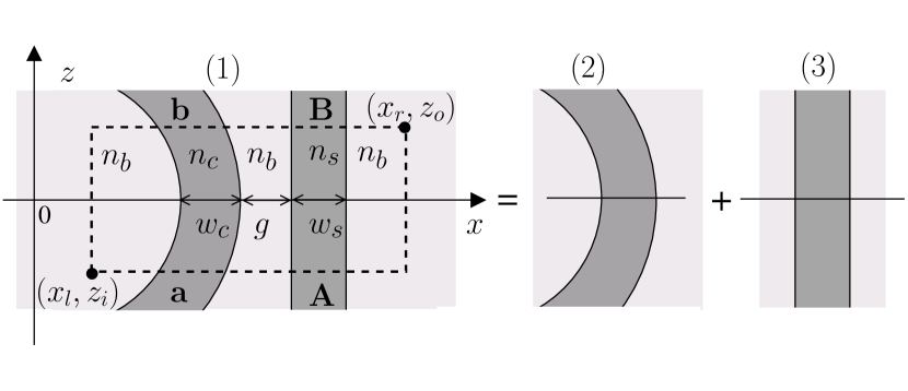
Figure 2: CMT setting for bent-straight waveguide couplers. The coupler is defined in the region $[x_{l},x_{r}]\times[z_{i},z_{o}]$. The external segments of the bent waveguide and the straight waveguide constitute the port connections. It is assumed that outside the coupler there is negligible interaction between the waveguides.

The field $\{\mathbf{E},\mathbf{H}\}$ inside the coupler is given by a linear combination of the modal fields of the bent waveguide (Fig. 2-(2)) and the modal fields of the straight waveguide (Fig. 2-(3)):

$$\vspace{-0.2cm}\begin{bmatrix}\mathbf{E}(x,z)\\ \mathbf{H}(x,z)\end{bmatrix}=\sum_{p=1}^{N_{b}}C_{b}^{p}(z)\begin{bmatrix}\mathbf{E}_{b}^{p}(x,z)\\ \mathbf{H}_{b}^{p}(x,z)\end{bmatrix}+\sum_{q=1}^{N_{s}}C_{s}^{q}(z)\begin{bmatrix}\mathbf{E}_{s}^{q}(x,z)\\ \mathbf{H}_{s}^{q}(x,z)\end{bmatrix},$$ (3)

where $C_{b}^{p}$, $C_{s}^{q}$ are unknown amplitudes. As shown in Ref. [4], a procedure based on the Lorentz reciprocity theorem leads to the following coupled mode equations

$$\mbox{\sf M}(x,z)\cdot d_{z}\mathbf{C}(z)=\mbox{\sf F}(x,z)\cdot\mathbf{C}(z),\vspace{-0.2cm}$$ (4)

with $\mbox{\sf M}_{ij}=\langle\mathbf{E}_{m}^{i},\mathbf{H}_{m}^{i};\mathbf{E}_{n}^{j},\mathbf{H}_{n}^{j}\rangle=\int\mathbf{a}_{z}\cdot(\mathbf{E}_{m}^{i}\times\mathbf{H}^{j*}_{n}+\mathbf{E}^{j*}_{n}\times\mathbf{H}_{m})dx$, $\mbox{\sf F}_{ij}=\int(\epsilon-\epsilon_{m})\mathbf{E}_{m}^{i}\cdot\mathbf{E}_{n}^{j*}dx$, $C_{i}=C_{m}^{i}$ for $i,j=1,2,\cdots,(N_{b}+N_{s})$, and $m=b$ if $1\leq i\leq N_{b}$ otherwise $m=s$, $n=b$ if $1\leq j\leq N_{b}$ otherwise $n=s$. Here $\mathbf{a}_{z}$ is a unit vector in $z$- direction and $\epsilon$ is the relative permittivity of the complete coupler. The integrations extend over $[x_{l},x_{r}]$ for each $z$ level.

Solving Eq. (4) by a Runge Kutta method of order 4, we get a relation $\mathbf{C}(z_{o})=\mbox{\sf T}\cdot\mathbf{C}(z_{i})$ between the amplitudes in the output and input coupler ports. For rather radiative bend modes, it takes a long $z$- distance to stabilize the elements of matrix T. This difficulty is overcome by taking the projections of the coupled fields onto the straight waveguide modes [4]. Then the output amplitudes of the straight waveguide modes are given by

$$B^{q}=\left[C_{s}^{q}(z_{o})+\left.\sum_{p=1}^{N_{b}}C_{b}^{p}(z_{o})\frac{\langle\mathbf{E}_{b}^{p},\mathbf{H}_{b}^{p};\mathbf{E}_{s}^{q},\mathbf{H}_{s}^{q}\rangle}{\langle\mathbf{E}_{s}^{q},\mathbf{H}_{s}^{q};\mathbf{E}_{s}^{q},\mathbf{H}_{s}^{q}\rangle}\right|_{z_{o}}\right]\mbox{e}^{-\mbox{i}\beta^{q}z_{o}}.$$ (5)

By incorporating these projection corrections into T, we finally obtain the required scattering matrix S.

Simulations and comparison

We consider a cavity in the form of a disk, i.e. $w_{c}=0$. Since the modal loss of the bend modes increases with growing mode order (where the order of the mode is defined as in Ref. [2]), one can expect that only the lower order bend modes play a dominant role for the field evolution in the cavity.

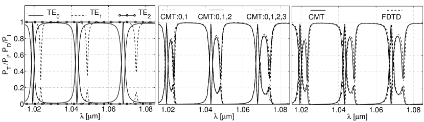
Figure 3: TE power spectrum for a 2D disk microresonator. Left: CMT with only a single (one of TE₀,TE₁ or TE₂) cavity mode. Middle: CMT results for two (dashed line), three (solid line) and four (dash-dotted line) cavity modes together. Right: Comparison of FDTD results and CMT results with 3 cavity modes. MR specifications: $n_{c}=n_{s}=1.5$, $n_{b}=1.0$, $w_{c}=0\ \,\mu\mbox{m}$ (disk), $w_{s}=0.4\ \,\mu\mbox{m}$, $R=5\ \,\mu\mbox{m}$, $g=0.2\ \,\mu\mbox{m}$.

The present CMT setting allows to investigate the significance of individual cavity modes for the spectral response of the MRs. The left plot of Fig. 3 shows the dropped power and the transmitted power when only a single cavity mode (either TE₀, TE₁ or TE₂) is included in the CMT model. The extrema corresponding to the fundamental mode (TE₀) are much more pronounced than those related to the first order mode (TE₁). If only the TE₂ cavity mode is taken into account, on the present scale hardly any variations of $P_{D}$ and $P_{T}$ appear. The middle plot of Fig. 3 shows the cumulative effect of the higher order cavity modes. The extrema corresponding to the fundamental mode remain almost unaffected, but the shape of the resonances related to the TE₁ mode changes. Note that the curves for three and four cavity modes almost coincide. The right plot of Fig. 3 compares the CMT results (3 cavity modes) with FDTD simulations [5]. The results agree surprisingly well.

Fig. 4 illustrates the field profiles for the full MR structure as predicted by the CMT. At the resonance corresponding to the fundamental mode, most of the input power is coupled to the fundamental cavity mode and appears at the drop port. For the resonance corresponding to the higher order modes, the circular nodal line in the field pattern in the cavity indicates that a significant part of the input power is coupled to the TE₁ mode. For an off resonance wavelength, most of the input power appears at the through port.

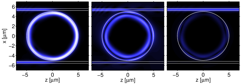
Figure 4: Absolute value of the $y$ component of TE fields of the MR. The gray scales (black = zero) are comparable among the plots. From left to right: MR field at a resonance corresponding to the fundamental mode ($\lambda=1.043\,\mu\mbox{m}$), a resonance corresponding to the higher modes ($\lambda=1.04833\,\mu\mbox{m}$) and off resonance ($\lambda=1.055\,\mu\mbox{m}$). CMT simulations ( 3 cavity modes) for a MR with the parameters as for Fig. 3.

Conclusions

The CMT based model of 2D microresonators yields quite accurate results even if few cavity modes are taken into account. These results agree well with the rigorous FDTD results and can be obtained with much lower computational effort. The role of the individual cavity modes can be clearly identified in this CMT model.

Cf. also the bibliography lists of Refs.[2]-[5].

References

- [1] Next generation active integrated optic subsystems (NAIS), project start: 2001. Information society technologies programme of the European Commission, project IST-2000-28018, http://www.mesaplus.utwente.nl/nais/.
- [2] K. R. Hiremath, M. Hammer, S. Stoffer, L. Prkna, and J. Čtyroký. Analytic approach to dielectric optical bent slab waveguides. Optical and Quantum Electronics. (accepted, 2004).
- [3] M. Hammer, K. R. Hiremath, and R. Stoffer. Analytical approaches to the description of optical microresonator devices. In M. Bertolotti, A. Driessen, and F. Michelotti, editors, Microresonators as building blocks for VLSI photonics, volume 709 of AIP conference proceedings, pages 48–71. American Institute of Physics, Melville, New York, 2004.
- [4] R. Stoffer, K. R. Hiremath, and M. Hammer. Comparison of coupled mode theory and FDTD simulations of coupl ing between bent and straight optical waveguides. pages 366–377 (same as above)
- [5] R. Stoffer. Uni- and Omnidirectional Simulation Tools for Integrated Optics. PhD thesis, University of Twente, Enschede, The Netherlands, May 2001.