Kinetic Limit for Wave Propagation in a Random Medium

Abstract

We study crystal dynamics in the harmonic approximation. The atomic masses are weakly disordered, in the sense that their deviation from uniformity is of order $\sqrt{\varepsilon}$. The dispersion relation is assumed to be a Morse function and to suppress crossed recollisions. We then prove that in the limit $\varepsilon\to 0$ the disorder averaged Wigner function on the kinetic scale, time and space of order $\varepsilon^{-1}$, is governed by a linear Boltzmann equation.

1 Introduction

When investigating the propagation of waves, one has to deal with the fact that the supporting medium often is not perfectly homogeneous, but suffers from irregularities. A standard method is then to assume that the material coefficients characterizing the medium are random, being homogeneous only in average. Examples abound: Shallow water waves travelling in a canal with uneven bottom, radar waves propagating through turbulent air, elastic waves dispersing in a random compound of two materials. The arguably simplest prototype is the scalar wave equation

$$n^{2}\partial_{t}^{2}u=c^{2}\Delta u$$ (1.1)

with a random index of refraction $n$. We will be interested in the case where the randomness is frozen in, or at most varies slowly on the time scale of the wave propagation. To say, we assume $x\mapsto n(x)$ to be a stationary stochastic process with short range correlations.

An important special case is a random medium with a small variance of $n(x)$, which one can write as

$$n(x)=(1+\sqrt{\varepsilon}\xi(x))^{-1}$$ (1.2)

with $\xi(x)$ order $1$ and $\varepsilon\ll 1$. As argued many times, ranging from isotope disordered harmonic crystals to seismic waves propagating in the crust of the Earth, for such weak disorder a kinetic description becomes possible and offers a valuable approximation to the complete equation (1.1) – we refer to the highly instructive survey by Ryzhik, Keller and Papanicolaou [16] for details. In the kinetic limit one considers times of order $\varepsilon^{-1}$ and spatial distances of order $\varepsilon^{-1}$. On that scale, the Wigner function $W$ associated to the solution $u$ of (1.1) is, in a good approximation, governed by the Boltzmann type transport equation

$$\partial_{t}W(x,k,t)+\nabla\omega(k)\cdot\nabla_{x}W(x,k,t)$$

$$\quad=\int\!{\rm d}k^{\prime}\left(r(k^{\prime},k)W(x,k^{\prime},t)-r(k,k^{\prime})W(x,k,t)\right).$$ (1.3)

Here $x\in{\mathbb{R}}^{3}$, the physical space, and $k$ denotes the wave number. $\omega$ is the dispersion relation, $\omega(k)=c|k|$ with $k\in{\mathbb{R}}^{3}$ for (1.1). Note that the left hand side of (1) is the semiclassical approximation to (1.1) with $n(x)=1$. The collision operator on the right hand side of (1) describes the scattering from the inhomogeneities with a rate kernel $r(k,k^{\prime}){\rm d}k^{\prime}$ which depends on the particular model under consideration.

Despite the wide use of the kinetic approximation (1), there is no complete mathematical justification for the step from microscopic equations like (1.1), together with (1.2), to (1) apart from one exception: Erdős and Yau [8] (see also [3, 4, 5, 6, 7]) investigate the random Schrödinger equation

$${\rm i}\partial_{t}\psi(x,t)=(-\Delta+\sqrt{\varepsilon}V)\psi(x,t),$$ (1.4)

where $\psi$ is the ${\mathbb{C}\hskip 0.21529pt}$-valued wave function. This equation can be thought of as a two component wave equation for our purposes. In [8] it is established that (1) becomes valid on the kinetic scale. Of course, the proof exploits special properties of the Schrödinger equation. For us one motivation leading to the present investigation was to understand whether the techniques developed in [8] carry over to standard wave equations such as (1.1). In fact, with the proper adjustments they do, and we are quite confident that also other wave equations with small random coefficients, as e.g. discussed in [16], can be treated in the same way. Due to the intricate nature of the estimates, we do not claim this to be an easy exercise, but there is a blue-print which now can be followed.

Even restricting to the scalar wave equation (1.1) there are choices to be made. One could add dispersion as $c^{2}(\Delta u-u)$ or the randomness could sit in the Laplacian as $\nabla\cdot(c(x)^{2}\nabla u)$ with $c(x)$ random and $n(x)=1$. To have a model of physical relevance, in our contribution we will consider a dielectric crystal in the harmonic approximation. If, for simplicity, the crystal structure is simple cubic, then $u_{y}$, $y\in{\mathbb{Z}}^{3}$, are the displacements of the atoms from their equilibrium position. Their movement is governed by Newton’s equations of motion

$$m_{y}\frac{{\rm d}^{2}}{{\rm d}t^{2}}u_{y}=(\Delta u)_{y},\qquad y\in{\mathbb{Z}}^{3}.$$ (1.5)

Here $\Delta$ is the lattice Laplacian, which corresponds to an elastic coupling between nearest neighbour atoms, and $m_{y}$ is the mass of the atom at $y$. (1.5) can be regarded as the space discretized version of (1.1). Real crystals come as isotope mixtures. For instance, natural silicon consists in 92.23% of ²⁸Si, 4.68% of ²⁹Si, and 3.09% of ³⁰Si. Thus $\text{Var}(m_{x})/\text{Av}(m_{x})^{2}\approx 10^{-4}$ and, in the appropriate units, we set

$$m_{y}=(1+\sqrt{\varepsilon}\,\xi_{y})^{-2},\qquad\varepsilon\ll 1,$$ (1.6)

where $\xi_{y}$, $y\in{\mathbb{Z}}^{3}$, are i.i.d. bounded, mean zero, random variables, in slight generalization of our example.

For the discretized wave equation the wave vector space is the unit torus ${\mathbb{T}}^{3}$. If $\omega$ denotes the dispersion relation for (1.5), the Boltzmann transport equation becomes

$$\partial_{t}W(x,k,t)+\frac{\nabla\omega(k)}{2\pi}\cdot\nabla_{x}W(x,k,t)$$

$$\quad=2\pi{\mathbb{E}}[\xi_{0}^{2}]\int\!{\rm d}k^{\prime}\omega(k^{\prime})^{2}\delta(\omega(k)-\omega(k^{\prime}))\left(W(x,k^{\prime},t)-W(x,k,t)\right).$$ (1.7)

We will establish that the disorder averaged Wigner function on the kinetic scale, space and time of order $\varepsilon^{-1}$, is governed by (1). In fact, we will allow for more general elastic couplings between the crystal atoms than given in (1.5). Our precise assumptions on $\omega$ will be discussed in Section 2.2.

In passing, let us remark that, to compute the thermal conductivity of real crystals, scattering from isotope disorder contributes only as one part. At least equally important are weak non-linearities in the elastic couplings, see [17] for an exhaustive discussion. In addition, at low temperatures, roughly below $100^{\circ}\text{K}$ for silicon, lattice vibrations have to be quantized. However, for isotope disorder as in (1.6) quantization would not make any difference, since the corresponding Heisenberg equations of motion are also linear.

In a loosely related work, Bal, Komorowski, and Ryzhik [2] study the high frequency limit of (1.1) and (1.2), under the assumption that the initial data vary on a space scale $\gamma^{-1}$ with $\gamma\ll\varepsilon\ll 1$. They prove that the Wigner function is well approximated by a transport equation of the form (1). Only the Boltzmann collision operator is to be replaced by its small angle approximation. Thus according to the limit equation the wave vector $k$ diffuses on the sphere $|k|=\text{\it const.}$, whereas in (1) it would be a random jump process. Their method is disjoint from ours and would not be able to cover the limiting case $\gamma=\varepsilon$. Bal et al. also prove self-averaging of the limit Wigner function, while our result will concern only the disorder averaged Wigner function. We expect however to have self-averaging of the Wigner function also in our case, see [4] for the corresponding result for the lattice random Schrödinger equation (1.4).

Wave propagation in a random medium has been studied also away from the weak disorder regime. As the main novelty, at strong disorder, and at any disorder in space dimension $1$, propagation is suppressed. The wave equation has localized eigenmodes. We refer to the review article [12]. The regime of extended eigenmodes is still unaccessible mathematically. The kinetic limit can be viewed as yielding some, even though rather modest, information on the delocalized eigenmodes, compare with [3].

In the following section we provide a more precise definition of the model, describe in detail our assumptions on the dispersion relation $\omega$ and on the initial conditions, and state the main result.

Acknowledgements

Our interest in wave propagation in random media where triggered by discussions of H.S. with H.-T. Yau during a common stay at the Institute for Advanced Study, Princeton in the spring 2003. We are grateful to László Erdős and Thomas Chen for their constant support and encouragement. We also thank A. Kupiainen, A. Mielke, G. Panati, and S. Teufel for instructive discussions.

J.L. acknowledges support from the Deutsche Forschungsgemeinschaft (DFG) project SP 181/19-1 and from the Academy of Finland in 2003. This work has also been supported by the European Commission through its 6th Framework Programme “Structuring the European Research Area” and the contract Nr. RITA-CT-2004-505493 for the provision of Transnational Access implemented as Specific Support Action.

2 Main result

2.1 Discrete wave equation

We will study the kinetic limit of the discrete wave equation

$$\frac{{\rm d}}{{\rm d}t}q_{y}(t) =v_{y}(t),$$

$$(1+\sqrt{\varepsilon}\,\xi_{y})^{-2}\frac{{\rm d}}{{\rm d}t}v_{y}(t) =-\sum_{y^{\prime}\in{\mathbb{Z}}^{3}}\alpha(y-y^{\prime})q_{y^{\prime}}(t)$$ (2.1)

with $y\in{\mathbb{Z}}^{3}$ and $q_{y}(t),v_{y}(t)\in{\mathbb{R}}$. As a shorthand we set $q(t)=(q_{y}(t),y\in{\mathbb{Z}}^{3})$, $v(t)=(v_{y}(t),y\in{\mathbb{Z}}^{3})$. The mass of the atom at site $y$ is $(1+\sqrt{\varepsilon}\,\xi_{y})^{-2}$, where $\xi=(\xi_{y},y\in{\mathbb{Z}}^{3})$ is a family of independent, identically distributed random variables. Their common distribution is independent of $\varepsilon$, has zero mean and is supported on the interval $[-\bar{\xi},\bar{\xi}]$. Expectation with respect to $\xi$ is denoted by ${\mathbb{E}}$. We assume $\varepsilon<\varepsilon_{0}=\bar{\xi}^{-2}$ throughout. Hence $1+\sqrt{\varepsilon}\,\xi_{y}>0$ with probability one.

The coefficients $\alpha(y)$ are the elastic couplings between atoms, and we require them to have the following properties.

• $\alpha(y)\neq 0$ for some $y\neq 0$.

• $\alpha(-y)=\alpha(y)$ for all $y$.

• There are constants $C_{1},C_{2}>0$ such that for all $y$

  $$|\alpha(y)|\leq C_{1}{\rm e}^{-C_{2}|y|}.$$ (2.2)

• Let $\smash{\widehat{\alpha}}$ be the Fourier transform of $\alpha$, which we define by

  $$\smash{\widehat{\alpha}}(k)=\sum_{y\in{\mathbb{Z}}^{3}}{\rm e}^{-{\rm i}2\pi k\cdot y}\alpha(y).$$ (2.3)

  Then $\smash{\widehat{\alpha}}:{\mathbb{T}}^{3}\to{\mathbb{R}}$, where ${\mathbb{T}}^{3}$ denotes the $3$-torus with unit side length. Mechanical stability demands $\smash{\widehat{\alpha}}\geq 0$. We require here the somewhat stronger condition

  $$\smash{\widehat{\alpha}}(k)>0,\quad\text{for all }k\in{\mathbb{T}}^{3}.$$ (2.4)

If $\varepsilon=0$, Eqs. (2.1) admit plane wave solutions with wave vector $k\in{\mathbb{T}}^{3}$ and frequency

$$\omega(k)=\sqrt{\smash{\widehat{\alpha}}(k)}.$$ (2.5)

The function $\omega:{\mathbb{T}}^{3}\to{\mathbb{R}}$ is the dispersion relation. Under our assumptions for $\alpha$, $\omega$ is real-analytic, $\omega(-k)=\omega(k)$, $0<\omega_{\text{min}}=\min_{k}\omega(k)$, and $\omega_{\text{max}}=\max_{k}\omega(k)<\infty$.

We solve the differential equations (2.1) as a Cauchy problem with initial data $q(0),v(0)$. The time-evolution (2.1) conserves the energy

$$E(q,v)=\frac{1}{2}\Bigl{(}\sum_{y\in{\mathbb{Z}}^{3}}(1+\sqrt{\varepsilon}\,\xi_{y})^{-2}v^{2}_{y}+\sum_{y,y^{\prime}\in{\mathbb{Z}}^{3}}\alpha(y-y^{\prime})q_{y}q_{y^{\prime}}\Bigr{)}.$$ (2.6)

The initial data are assumed to have finite energy, $E(q(0),v(0))<\infty$. Since $\omega_{\text{min}}>0$, this implies that $q(0),v(0)\in\ell_{2}({\mathbb{Z}}^{3},{\mathbb{R}})$. For any realization of $\xi$, the generator of the time-evolution (2.1) is a bounded operator on $\ell_{2}({\mathbb{Z}}^{3},{\mathbb{R}}^{2})$. Therefore, the Cauchy problem has a unique, norm-continuous solution which remains in $\ell_{2}({\mathbb{Z}}^{3},{\mathbb{R}}^{2})$ for all $t\in{\mathbb{R}}$.

The energy depends on the realization of $\xi$, and it will be more convenient to switch to new variables such that the flat $\ell_{2}$-norm is conserved. For this purpose, let tilde denote the inverse Fourier transform, for which we adopt the convention

$$\smash{\widetilde{f}}_{y}=\int_{{\mathbb{T}}^{3}}\!{\rm d}k\,{\rm e}^{{\rm i}2\pi y\cdot k}f(k),$$ (2.7)

and let $\Omega$ denote the bounded operator on $\ell_{2}({\mathbb{Z}}^{3},{\mathbb{C}\hskip 0.21529pt})$ defined via

$$(\Omega\phi)_{y}=\sum_{y^{\prime}\in{\mathbb{Z}}^{3}}\smash{\widetilde{\omega}}_{y-y^{\prime}}\phi_{y^{\prime}}.$$ (2.8)

Since $q(t),v(t)\in\ell_{2}({\mathbb{Z}}^{3},{\mathbb{R}})$, we can introduce the vector $\psi(t)\in\ell_{2}({\mathbb{Z}}^{3},{\mathbb{C}\hskip 0.21529pt}^{2})$ through

$$\psi(t)_{\sigma,y}=\frac{1}{2}\left((\Omega q(t))_{y}+{\rm i}\sigma(1+\sqrt{\varepsilon}\,\xi_{y})^{-1}v(t)_{y}\right),$$ (2.9)

where $\sigma=\pm 1$ and $y\in{\mathbb{Z}}^{3}$. From now on, let us denote $\ell_{2}=\ell_{2}({\mathbb{Z}}^{3},{\mathbb{C}\hskip 0.21529pt})$, and $\mathcal{H}=\ell_{2}({\mathbb{Z}}^{3},{\mathbb{C}\hskip 0.21529pt}^{2})=\ell_{2}\oplus\ell_{2}$.

If we regard $\xi$ as a multiplication operator on $\ell_{2}$, i.e., if we define $(\xi\psi)_{y}=\xi_{y}\psi_{y}$, then $\psi(t)$ satisfies the differential equation

$$\frac{{\rm d}}{{\rm d}t}\psi(t)=-{\rm i}H_{\varepsilon}\psi(t),\quad\text{with}\quad H_{\varepsilon}=H_{0}+\sqrt{\varepsilon}V,$$ (2.10)

where

$$H_{0}=\begin{pmatrix}\Omega&0\\ 0&-\Omega\end{pmatrix},\quad V=\frac{1}{2}\begin{pmatrix}\Omega\xi+\xi\Omega&-\Omega\xi+\xi\Omega\\ \Omega\xi-\xi\Omega&-\Omega\xi-\xi\Omega\end{pmatrix}.$$ (2.11)

Because $H_{\varepsilon}$ is a self-adjoint operator on $\mathcal{H}$, the solution to (2.10) generates a unitary group on $\mathcal{H}$. Unitarity is equivalent to energy conservation, since for all $t$

$$\|\psi(t)\|^{2}=E(q(t),p(t)).$$ (2.12)

If $\psi(t)$ is one of the “physical” states obtained by (2.9), then it satisfies $\psi(t)_{-,y}^{*}=\psi(t)_{+,y}$ for all $y$ and $t$ due to $q(t),v(t)\in{\mathbb{R}}$. We will discuss in Section 7 how information about $\psi(t)$ is transferred to $q(t)$, $v(t)$.

2.2 Lattice Wigner function, initial conditions, and dispersion relation

The disorder has strength $\sqrt{\varepsilon}$. Since ${\mathbb{E}}[\xi_{0}]=0$, effects of order $\sqrt{\varepsilon}$ vanish in the mean, and a wave packet has a mean free path of the order of $\varepsilon^{-1}$ lattice spacings. In the kinetic limit the speed of propagation of the waves is independent of $\varepsilon$, indicating that the first time-scale, at which the randomness becomes relevant, is also of the order of $\varepsilon^{-1}$. If $\xi=0$, this scaling corresponds to the semiclassical limit in which the Wigner function satisfies the transport equation

$$\partial_{t}W(x,k,t)+\frac{\nabla\omega(k)}{2\pi}\cdot\nabla_{x}W(x,k,t)=0,\quad x\in{\mathbb{R}}^{3},\ k\in{\mathbb{T}}^{3}.$$ (2.13)

We refer to [14] for an exhaustive discussion. From this perspective, the Wigner function is the natural object for studying the kinetic limit.

Given a scale $\varepsilon>0$, we define the Wigner function $W^{\varepsilon}$ of any state $\psi\in\mathcal{H}$ as the distributional Fourier transform

$$W_{\sigma^{\prime}\sigma}^{\varepsilon}(x,k)=\int_{{\mathbb{R}}^{3}}\!\!{\rm d}p\,{\rm e}^{{\rm i}2\pi x\cdot p}\smash{\widehat{\psi}}_{\sigma^{\prime}}\Bigl{(}k-\frac{1}{2}\varepsilon p\Bigr{)}^{*}\smash{\widehat{\psi}}_{\sigma}\Bigl{(}k+\frac{1}{2}\varepsilon p\Bigr{)},$$ (2.14)

where $\sigma^{\prime},\sigma\in\{\pm 1\}$, $x\in{\mathbb{R}}^{3}$, $k\in{\mathbb{T}}^{3}$. This is also called the Wigner transform of $\psi$ and we denote it by $W^{\varepsilon}[\psi]$. The Fourier transform of $\psi$, denoted by $\smash{\widehat{\psi}}$, is defined as in (2.3) and periodically extended to a function on the whole of ${\mathbb{R}}^{3}$. $W$ is an Hermitian ${\mathbb{M}}_{2}$-valued (complex $2{\times}2$-matrix) distribution. When integrated against a matrix-valued test-function $J\in\mathcal{S}({\mathbb{R}}^{3}\times{\mathbb{T}}^{3},{\mathbb{M}}_{2})$, (2.14) becomes

$$\langle J,W^{\varepsilon}\rangle=\int_{{\mathbb{R}}^{3}}\!\!{\rm d}p\int_{{\mathbb{T}}^{3}}\!\!{\rm d}k\,\smash{\widehat{\psi}}\Bigl{(}k-\frac{1}{2}\varepsilon p\Bigr{)}\cdot\smash{\widehat{J}}(p,k)^{*}\smash{\widehat{\psi}}\Bigl{(}k+\frac{1}{2}\varepsilon p\Bigr{)},$$ (2.15)

where $\smash{\widehat{J}}$ denotes the Fourier transform of $J$ in the first variable,

$$\smash{\widehat{J}}(p,k)=\int_{{\mathbb{R}}^{3}}\!{\rm d}x\,{\rm e}^{-{\rm i}2\pi p\cdot x}J(x,k).$$ (2.16)

The notation $A^{*}$ denotes Hermitian conjugation, and the dot is used for a finite-dimensional scalar product: $a\cdot b=\sum_{i}a_{i}^{*}b_{i}$. We have included a complex conjugation of the test-function in the definition in order to have the same sign convention for the Fourier transform of both test functions and distributions.

Let us choose now some initial conditions for (2.10). In general, it will be $\varepsilon$-dependent and we denote it by $\psi^{\varepsilon}$. The solution to (2.10) is then

$$\psi(t)={\rm e}^{-{\rm i}tH_{\varepsilon}}\psi^{\varepsilon}.$$ (2.17)

In the following we will be studying a limit where $\varepsilon\to 0^{+}$ via some arbitrary sequence of values. Our assumptions on the initial conditions are

Assumption 2.1 (Initial conditions)

For every $\varepsilon$, there is $\psi^{\varepsilon}\in\mathcal{H}$, independent of $\xi$, such that

• $\displaystyle\sup_{\varepsilon}\|\psi^{\varepsilon}\|<\infty$.

• $\displaystyle\lim_{R\to\infty}\limsup_{\varepsilon\to 0}\sum_{|y|>R/\varepsilon}|\psi^{\varepsilon}_{y}|^{2}=0$.

• There exists a positive bounded Borel measure $\mu_{0}$ on ${\mathbb{R}}^{3}\times{\mathbb{T}}^{3}$ such that

  $$\lim_{\varepsilon\to 0}\langle J,W^{\varepsilon}_{++}[\psi^{\varepsilon}]\rangle=\int_{{\mathbb{R}}^{3}\times{\mathbb{T}}^{3}}\!\!\mu_{0}({\rm d}x\,{\rm d}k)\,J(x,k)^{*}.$$ (2.18)

  for all $J\in\mathcal{S}({\mathbb{R}}^{3}\times{\mathbb{T}}^{3})$.

These assumptions are rather weak. In fact, as discussed in the Appendix B, if we assume (IC1), then the existence of the limit in (2.18) for all $J$ implies already the existence of the measure $\mu_{0}$. The condition (IC2) means that the sequence $|\psi^{\varepsilon}_{y}|^{2}/\|\psi^{\varepsilon}\|^{2}$ of probability measures on ${\mathbb{Z}}^{3}$ is tight on the kinetic scale $\varepsilon^{-1}$.

Our second set of assumptions deals with the dispersion relation $\omega$. For this we need to introduce the notations

$$\langle x\rangle=\sqrt{1+x^{2}}\qquad\text{and}\qquad\|f\|_{N,\infty}=\sup_{|\alpha|\leq N}\|D^{\alpha}\!f\|_{\infty},$$ (2.19)

where $N=0,1,\ldots$ and $\alpha$ denotes a multi-index.

Assumption 2.2 (Dispersion relation)

Let $\omega:{\mathbb{T}}^{3}\to{\mathbb{R}}$ satisfy all of the following:

• $\omega$ is smooth and $\omega(-k)=\omega(k)$.

• $\omega_{\text{min}}>0$ and $\omega_{\text{max}}<\infty$ with $\omega_{\text{min}}=\min_{k}\omega(k)$ and $\omega_{\text{max}}=\max_{k}\omega(k)$.

• (dispersivity)  There are constants $d_{1}\in{\mathbb{N}}$ and $c_{\omega}>0$ such that for all $t\in{\mathbb{R}}$ and $f\in C^{\infty}({\mathbb{T}}^{3})$,

  $$\left|\int_{{\mathbb{T}}^{3}}{\rm d}k\,f(k){\rm e}^{-{\rm i}t\omega(k)}\right|\leq\frac{c_{\omega}}{\langle t\rangle^{3/2}}\|f\|_{d_{1},\infty}.$$ (2.20)

• (crossings are suppressed)  There are constants $c_{2}>0$, $0<\gamma\leq 1$ and $d_{2}\in{\mathbb{N}}$ such that for all $u\in{\mathbb{T}}^{3}$, $0<\beta\leq 1$, $\alpha\in{\mathbb{R}}^{3}$, and $\sigma\in\{\pm 1\}^{3}$,

  $$\int_{({\mathbb{T}}^{3})^{2}}{\rm d}k_{1}{\rm d}k_{2}\,\frac{1}{|\alpha_{1}-\sigma_{1}\omega(k_{1})+{\rm i}\beta||\alpha_{2}-\sigma_{2}\omega(k_{2})+{\rm i}\beta|}$$

  $$\qquad\times\frac{1}{|\alpha_{3}-\sigma_{3}\omega(k_{1}-k_{2}+u)+{\rm i}\beta|}\leq c_{2}\beta^{\gamma-1}\langle\ln\beta\rangle^{d_{2}}.$$ (2.21)

If $\omega$ has only isolated, non-degenerate critical points, i.e., if $\omega$ is a Morse function, then the bound (2.20) with $d_{1}=4$ follows by standard stationary phase methods. The crossing condition is more difficult to verify. We will discuss these issues in detail in Sec. 6, where examples satisfying (DR3) and (DR4) are also provided.

2.3 Main Theorem

The Boltzmann equation (1) is the forward equation of a Markov jump process $(x(t),k(t))$, $t\geq 0$. $k(t)$, $t\geq 0$ is governed by the collision rate

$$\nu_{k}({\rm d}k^{\prime})={\rm d}k^{\prime}\delta(\omega(k)-\omega(k^{\prime}))2\pi{\mathbb{E}}[\xi_{0}^{2}]\omega(k^{\prime})^{2},\quad k\in{\mathbb{T}}^{3},$$ (2.22)

with a total collision rate

$$\sigma(k)=\nu_{k}({\mathbb{T}}^{3}).$$ (2.23)

As proved in Appendix A, since $\omega$ is continuous and (DR3) is satisfied, the map

$$k\mapsto\int\!\nu_{k}({\rm d}k^{\prime})g(k^{\prime})$$ (2.24)

is continuous for every $g\in C({\mathbb{T}}^{3})$. In particular, $\sigma_{\text{max}}=\sup_{k}\sigma(k)<\infty$. Now given $k=k(0)$, one has $k(t)=k$ for $0\leq t\leq\tau$ with $\tau$ an exponentially distributed random variable of mean $\sigma(k)^{-1}$. At time $\tau$, $k$ jumps to ${\rm d}k^{\prime}$ with probability $\nu_{k}({\rm d}k^{\prime})/\sigma(k)$, etc. To define the joint process $(x(t),k(t))$, $t\geq 0$, one sets

$$\frac{{\rm d}}{{\rm d}t}x(t)=\frac{1}{2\pi}\nabla\omega(k(t)).$$ (2.25)

We assume the process to start in the measure $\mu_{0}$ from (IC3). Because of continuity in (2.24), the process $(x(t),k(t))$, $t\geq 0$, is Feller. Hence there is a well-defined joint distribution at time $t$, which we denote by $\mu_{t}({\rm d}x\,{\rm d}k)$.

We are now ready to state our main result.

Theorem 2.3

Let the Assumptions 2.1 and 2.2 hold and let $\psi(t)$ denote the random vector determined by (2.17). Then for all $t\geq 0$, $J\in\mathcal{S}({\mathbb{R}}^{3}\times{\mathbb{T}}^{3})$, one has the limit

$$\lim_{\varepsilon\to 0}{\mathbb{E}}[\langle J,W_{++}^{\varepsilon}[\psi(t/\varepsilon)]\rangle]=\int_{{\mathbb{R}}^{3}\times{\mathbb{T}}^{3}}\!\!\mu_{t}({\rm d}x\,{\rm d}k)\,J(x,k)^{*}.$$ (2.26)

As a complete theorem, one would have expected a limit for the Wigner matrix, not just for the ($++$)-component, as stated above. From the evolution equation (2.10) it follows immediately that Theorem 2.3 also holds for $W_{--}$. One only has to assume (IC3) for $W_{--}^{\varepsilon}$, and replace everywhere $\omega$ by $-\omega$. As the rate kernel remains unchanged, this amounts to changing the sign in (2.25). For the deterministic initial data of Section 2.1 the off-diagonal components $W^{\varepsilon}_{+-}$ and $W^{\varepsilon}_{-+}$ are fastly oscillating. In general, they do not have a pointwise limit, but vanish upon time-averaging, i.e., for any $t\geq 0$, $T>0$ and $\sigma=\pm 1$, one has

$$\lim_{\varepsilon\to 0}\frac{1}{T}\int_{0}^{T}\!\!{\rm d}\tau\,{\mathbb{E}}\!\left[W^{\varepsilon}_{\sigma,-\sigma}[\psi((t+\tau)/\varepsilon)]\right]=0.$$ (2.27)

Physically, one would like to avoid the assumption $\omega_{\text{min}}>0$, since elastic forces depend only on the relative distances between atoms, and thus $\smash{\widehat{\alpha}}(0)=0$. If $\smash{\widehat{\alpha}}(0)=0$, generically $\omega(k)\approx|k|$ for small $k$. In addition, by (2.11), the two bands of $H_{0}$ touch at $k=0$. On a technical level, the non-smooth crossing of the bands adds another layer of difficulty which we wanted to avoid here.

To give a brief outline: In the following section we exploit general properties about weak limits of lattice Wigner transforms to reduce the proof of the main theorem into a Proposition stating that their Fourier transforms converge to the characteristic functions of $(\mu_{t})$. These properties concerning the Wigner transform are valid under more general assumptions than those of the main theorem, and we have separated their derivation to Appendix B. The core of the paper is the graphical expansion of Section 4 where the proof of the above Proposition is done by dividing it into several layers with ever more detailed Lemmas acting as links between the different layers. In particular, we have separated the analysis of the non-vanishing parts of the graph expansion, so called simple graphs, to Section 5.

The graph expansion follows the outline laid down in the works cited earlier. The new ingredients are the matrix structure and the momentum dependence of the interaction. We also develop here an alternative version for the so-called partial time-integration needed in the estimation of the error terms. The present version, described in Sec. 4.1, facilitates the analysis of the error terms, allowing the use of same estimates for both partially time-integrated and fully expanded graphs. We also consider here more general dispersion relations and initial conditions than before, although it needs to be stressed that in the case of the dispersion relation, the improvement is mainly a matter of more careful bookkeeping.

The estimates, which allow the division of the graphs into leading and subleading ones, rely on the decay estimates (DR3) and (DR4). In section 6 we discuss proving (DR4) for a given dispersion relation in more detail. In particular, we show there that the taking of the square root, which is necessary for obtaining the dispersion relation from the elastic couplings, in general retains the validity of the crossing estimate. Finally, in the last section we return to the original lattice dynamics (2.1), explain how (IC1) – (IC3) relate to the initial positions and velocities, and, in particular, discuss the propagation of the energy density.

3 Proof of the Main Theorem

In all of the results in this and the following two sections, unless stated otherwise, we make the assumptions of Theorem 2.3. In addition, we assume that ${\mathbb{E}}[\xi_{0}^{2}]=1$. This is not a restriction, as it can always be achieved by rescaling $\xi$ by ${\mathbb{E}}[\xi_{0}^{2}]^{-\frac{1}{2}}$ and $\varepsilon$ by ${\mathbb{E}}[\xi_{0}^{2}]$. We study a given sequence $(\varepsilon_{k})$, $k=1,2,\ldots$, such that $0<\varepsilon_{k}<\varepsilon_{0}$ and $\lim_{k}\varepsilon_{k}=0$. For notational simplicity, we will always denote the limits of the type $\lim_{k\to\infty}f(\varepsilon_{k})$ by $\lim_{\varepsilon\to 0}f(\varepsilon)$.

We will study the limits of the mappings $\overline{W}^{\varepsilon}\!(t)$ defined by $\langle J,\overline{W}^{\varepsilon}\!(t)\rangle={\mathbb{E}}[\langle J,W_{++}^{\varepsilon}[\psi(t/\varepsilon)]\rangle]$ where $\psi(t)={\rm e}^{-{\rm i}H_{\varepsilon}t}\psi^{\varepsilon}$. For any $\varepsilon$ and $t\geq 0$, the mapping $\xi\mapsto\psi(t/\varepsilon)$ lifts the probability measure for $\xi$ to a probability measure $\nu^{\varepsilon}_{t}$ on the Hilbert space $\mathcal{H}$. For instance, $\nu^{\varepsilon}_{0}$ is a Dirac measure concentrated at $\psi^{\varepsilon}$. Each of the measures $\nu^{\varepsilon}_{t}$ is a weak Borel measure. In particular, let us prove next that every $\psi(t/\varepsilon)_{\sigma,y}$ is measurable. For any $R>0$, define $V^{R}$ as the potential obtained by neglecting far lying perturbations $\xi$, i.e., let

$$V^{R}=\sum_{\|y\|_{\infty}\leq R}\xi_{y}V^{(y)}$$ (3.1)

where $V^{(y)}$, $y\in{\mathbb{Z}}^{3}$, has a Fourier transform given by the integral kernel

$$\smash{\widehat{V}}^{(y)}_{\sigma^{\prime}\sigma}(k^{\prime},k)={\rm e}^{-{\rm i}2\pi y\cdot(k^{\prime}-k)}v_{\sigma^{\prime}\sigma}(k^{\prime},k),$$ (3.2)

and $v\in L^{2}({\mathbb{T}}^{3}\times{\mathbb{T}}^{3},{\mathbb{M}}_{2})$ is defined for $\sigma^{\prime},\sigma\in\{\pm 1\}$ and $k^{\prime},k\in{\mathbb{T}}^{3}$ by

$$v_{\sigma^{\prime}\sigma}(k^{\prime},k)=\frac{\sigma^{\prime}\sigma}{2}\left(\sigma^{\prime}\omega(k^{\prime})+\sigma\omega(k)\right).$$ (3.3)

Then $V^{R}\to V$ strongly (i.e., for all $\psi\in\mathcal{H}$, $\|V^{R}\psi-V\psi\|\to 0$) when $R\to\infty$, and, as $\sup_{R}\|V^{R}\|<\infty$, the same is true for any product of $V^{R}$:s and bounded $R$-independent operators. Therefore,

$$\psi(t/\varepsilon)_{\sigma,y}=\lim_{R\to\infty}\sum_{N=0}^{R}\frac{(-{\rm i}t/\varepsilon)^{N}}{N!}((H_{0}+\sqrt{\varepsilon}V^{R})^{N}\psi^{\varepsilon})_{\sigma,y}.$$ (3.4)

As the summand is a complex function depending only on finitely many of $(\xi_{y})$, it is measurable. For all $|\xi|\leq\bar{\xi}$, $\psi(t/\varepsilon)_{\sigma,y}$ is a convergent limit of a sequence of such functions, which implies that also $\psi(t/\varepsilon)_{\sigma,y}$ is measurable. In addition, by the unitarity of ${\rm e}^{-{\rm i}H_{\varepsilon}t}$,

$$\|\psi(t/\varepsilon)\|^{2}=\|\psi^{\varepsilon}\|^{2}$$ (3.5)

which is uniformly bounded by (IC1).

By Theorem B.2, $\langle J,W_{\nu_{t}^{\varepsilon}}^{\varepsilon}\rangle=\int\!\nu_{t}^{\varepsilon}({\rm d}\psi)\langle J,W^{\varepsilon}[\psi]\rangle$ defines a distribution in $\mathcal{S}^{\prime}({\mathbb{R}}^{3}\times{\mathbb{T}}^{3},{\mathbb{M}}^{2})$ which we call the Wigner transform of the measure $\nu_{t}^{\varepsilon}$. These distributions behave very similarly to probability measures on ${\mathbb{R}}^{3}\times{\mathbb{T}}^{3}$, and we have collected their main properties in Appendix B. In particular, we can conclude that $\overline{W}^{\varepsilon}\!(t)\in\mathcal{S}^{\prime}({\mathbb{R}}^{3}\times{\mathbb{C}\hskip 0.21529pt}^{3})$, as for all $J\in\mathcal{S}({\mathbb{R}}^{3}\times{\mathbb{C}\hskip 0.21529pt}^{3})$,

$$\langle J,\overline{W}^{\varepsilon}\!(t)\rangle=\langle J,(W_{\nu_{t}^{\varepsilon}}^{\varepsilon})_{++}\rangle=\int\!\nu_{t}^{\varepsilon}({\rm d}\psi)\langle J,W^{\varepsilon}[\psi_{+}]\rangle.$$ (3.6)

By Proposition B.3, the Fourier transform of $\overline{W}^{\varepsilon}\!(t)$ is determined by the functions

$$F^{\varepsilon}_{t}(p,n)={\mathbb{E}}_{\nu_{t}^{\varepsilon}}\!\!\left[\int_{{\mathbb{T}}^{3}}\!\!{\rm d}k\,{\rm e}^{{\rm i}2\pi n\cdot k}\smash{\widehat{\psi}}_{+}\!\Bigl{(}k-\frac{1}{2}\varepsilon p\Bigr{)}^{*}\smash{\widehat{\psi}}_{+}\!\Bigl{(}k+\frac{1}{2}\varepsilon p\Bigr{)}\right]$$ (3.7)

where $p\in{\mathbb{R}}^{3}$ and $n\in{\mathbb{Z}}^{3}$. The assumptions (IC1) – (IC3) allow then applying Theorem B.4 to conclude that $F^{\varepsilon}_{0}$ converges pointwise to the Fourier transform of $\mu_{0}$ which, by Theorem B.5, implies

Lemma 3.1

For all $p\in{\mathbb{R}}^{3}$ and $f\in C({\mathbb{T}}^{3})$,

$$\lim_{\varepsilon\to 0}\int_{{\mathbb{T}}^{3}}\!\!{\rm d}kf(k)\,\smash{\widehat{\psi}}^{\varepsilon}_{+}\!\Bigl{(}k-\frac{1}{2}\varepsilon p\Bigr{)}^{*}\smash{\widehat{\psi}}^{\varepsilon}_{+}\!\Bigl{(}k+\frac{1}{2}\varepsilon p\Bigr{)}=\int_{{\mathbb{R}}^{3}\times{\mathbb{T}}^{3}}\!\!\!\!\mu_{0}({\rm d}x\,{\rm d}k)\,{\rm e}^{-{\rm i}2\pi p\cdot x}f(k).$$ (3.8)

Using time-dependent perturbation expansion, we will prove in Section 4 that

Proposition 3.2

For all $\bar{t}>0$, $\bar{p}\in{\mathbb{R}}^{3}$ and $\bar{n}\in{\mathbb{Z}}^{3}$

$$\lim_{\varepsilon\to 0}F^{\varepsilon}_{\bar{t}}(\bar{p},\bar{n})=\int_{{\mathbb{R}}^{d}\times{\mathbb{T}}^{d}}\!\!\!\!\mu_{\bar{t}}({\rm d}x\,{\rm d}k)\,{\rm e}^{-{\rm i}2\pi(\bar{p}\cdot x-\bar{n}\cdot k)}.$$ (3.9)

Then we can apply Theorem B.5, and conclude that for any $t>0$, the sequence $(\overline{W}^{\varepsilon}\!(t))_{\varepsilon}$ converges in the weak-$*$ topology to a bounded positive Borel measure whose characteristic function coincides with the limit of $F^{\varepsilon}_{t}$. However, then by (3.9) this measure is in fact equal to $\mu_{t}$. This is sufficient to prove Theorem 2.3, since (2.26) is valid at $t=0$ by assumption (IC3).

4 Graph expansion (proof of Proposition 3.2)

In this section we assume that all assumptions of Proposition 3.2 are valid. In particular, $\bar{p}\in{\mathbb{R}}^{3}$, $\bar{n}\in{\mathbb{Z}}^{3}$ and $\bar{t}>0$ will denote the fixed macroscopic parameters. We first derive, using time-dependent perturbation theory, a way of splitting the time-evolved states into two parts,

$${\rm e}^{-{\rm i}tH_{\varepsilon}}\psi^{\varepsilon}=\psi_{\text{main}}(t)+\psi_{\text{err}}(t).$$ (4.1)

The splitting is done in such the way that each part is component-wise measurable, as before, and

$$\lim_{\varepsilon\to 0}{\mathbb{E}}\!\left[\|\psi_{\text{err}}(\bar{t}/\varepsilon)\|^{2}\right]=0.$$ (4.2)

Then we will only need to inspect the limit of the main part.

4.1 Duhamel expansion with soft partial time-integration

We begin by deriving the above splitting. Since both $H_{0}$ and $V$ are bounded operators for any realization of the randomness, the Duhamel formula states that, for any $t\in{\mathbb{R}}$ we have as vector valued integrals in $\mathcal{B}(\mathcal{H})$,

$${\rm e}^{-{\rm i}tH_{\varepsilon}}={\rm e}^{-{\rm i}tH_{0}}+\int_{0}^{t}\!\!{\rm d}s\,{\rm e}^{-{\rm i}(t-s)H_{\varepsilon}}(-{\rm i}\sqrt{\varepsilon}V){\rm e}^{-{\rm i}sH_{0}}.$$ (4.3)

This could be iterated to yield the full Dyson series which, however, would become ill-behaved in the kinetic limit. Instead, we will expand the series only partially, up to $N_{0}$ “collisions”. For the remainder we use a different method, essentially a version of the “partial time integration” introduced in [8] with a “soft cut-off” which allows easier analysis of the error terms. The results will be expressed in terms of the following (random) functions:

Definition 4.1

For any $\varepsilon$, and any $\kappa\geq 0$ and $s\in{\mathbb{R}}$ let

$$W_{s} =(-{\rm i}\sqrt{\varepsilon}V){\rm e}^{-{\rm i}sH_{0}}\qquad\text{and}\qquad W_{s,\kappa}=(-{\rm i}\sqrt{\varepsilon}V){\rm e}^{-{\rm i}s(H_{0}-{\rm i}\kappa)},$$ (4.4)

and define for any $\kappa\geq 0$, $t>0$, and $N,N^{\prime},N_{0}\in{\mathbb{N}}$ with $N_{0}\geq 1$, as vector valued integrals in $\mathcal{B}(\mathcal{H})$,

$$F_{N}(t;\varepsilon) =\int_{{\mathbb{R}}_{+}^{N+1}}\!{\rm d}s\,\delta\Bigl{(}t-\sum_{\ell=1}^{N+1}s_{\ell}\Bigr{)}{\rm e}^{-{\rm i}s_{N+1}H_{0}}W_{s_{N}}\cdots W_{s_{1}},$$ (4.5)

$$G_{N^{\prime},N}(t;\varepsilon,\kappa) =\int_{{\mathbb{R}}_{+}^{N+N^{\prime}+1}}\!\!\!\!\!\!\!\!\!\!\!{\rm d}s\,\delta\Bigl{(}t-\!\!\!\!\sum_{\ell=1}^{N+N^{\prime}+1}\!\!\!\!s_{\ell}\Bigr{)}{\rm e}^{-{\rm i}s_{N+N^{\prime}+1}(H_{0}-{\rm i}\kappa)}\!\prod_{j=N+1}^{N+N^{\prime}}\!\!\!\!W_{s_{j},\kappa}\prod_{j=1}^{N}W_{s_{j}},$$ (4.6)

$$A_{N^{\prime},N_{0}}(t;\varepsilon,\kappa) =\int_{{\mathbb{R}}_{+}^{N_{0}+N^{\prime}}}\!{\rm d}s\,\delta\Bigl{(}t-\sum_{\ell=1}^{N_{0}+N^{\prime}}s_{\ell}\Bigr{)}\prod_{j=N_{0}+1}^{N_{0}+N^{\prime}}W_{s_{j},\kappa}\prod_{j=1}^{N_{0}}W_{s_{j}}.$$ (4.7)

Let us also define

$$F_{N}(0;\varepsilon)=\delta_{N0}\mathbbm{1},\quad G_{N^{\prime},N}(0;\varepsilon,\kappa)=\delta_{N+N^{\prime},0}\mathbbm{1},\quad\text{and}\quad A_{N^{\prime},N_{0}}(0;\varepsilon,\kappa)=0.$$ (4.8)

In these definitions, the notation ${\rm d}s\,\delta(t-\sum_{\ell=1}^{N}s_{\ell})$, with $t>0$ and $N\in{\mathbb{N}}_{+}$, refers to a bounded positive Borel measure on ${\mathbb{R}}_{+}^{N}$ defined naturally by the $\delta$-function by integrating out one of the coordinates $s_{\ell}$. Explicitly, for any $f\in C({\mathbb{R}}^{N})$ we have, for $N=1$, $\int_{0}^{\infty}\!{\rm d}s\,\delta(t-s)f(s)=f(t)$, and for $N\geq 1$,

$$\int_{{\mathbb{R}}_{+}^{N}}\!\!{\rm d}s\,\delta\Bigl{(}t-\sum_{\ell=1}^{N}s_{\ell}\Bigr{)}f(s)=\int_{{\mathbb{R}}_{+}^{N-1}}\!\!\!\!\!\!\!{\rm d}s\,\mathbbm{1}\!\Bigl{(}\sum_{\ell=1}^{N-1}s_{\ell}\leq t\Bigr{)}f\Bigl{(}s_{1},\ldots,s_{N-1},t-\sum_{\ell=1}^{N-1}s_{\ell}\Bigr{)}.$$ (4.9)

The function $\mathbbm{1}$ in the integrand restricts the integration region to the standard simplex in ${\mathbb{R}}^{N-1}$ scaled by the factor $t$. This is a compact set and therefore, as long as the integrand is a continuous mapping from the simplex to a Fréchet  space, it can be used to define vector valued integrals in the sense of [15], Theorem 3.27. The measure is invariant under permutations of $(s_{\ell})$ – which proves that we could have integrated out any of the coordinates, not only the last one – and it is bounded by

$$\int_{{\mathbb{R}}_{+}^{N}}\!{\rm d}s\,\delta\Bigl{(}t-\sum_{\ell=1}^{N}s_{\ell}\Bigr{)}=\frac{t^{N-1}}{(N-1)!}.$$ (4.10)

The proof that the integrands in the Definition 4.1 are continuous, as well as a number of useful relations between the functions, are given in the following:

Lemma 4.2

$W_{s}$ and $W_{s,\kappa}$ are continuous in $\mathcal{B}(\mathcal{H})$ in the variable $s$, as well as are all of the functions defined in (4.5) – (4.8) in $t$. They are also related by the following equalities for all $N_{0}\geq 1$ and $N^{\prime},N\geq 0$:

$$F_{N}(t;\varepsilon) =G_{0,N}(t;\varepsilon,0),$$ (4.11)

$$F_{N_{0}}(t;\varepsilon) =\int_{0}^{t}\!\!{\rm d}r\,{\rm e}^{-{\rm i}(t-r)H_{0}}A_{0,N_{0}}(r;\varepsilon,\kappa),$$ (4.12)

$$G_{N^{\prime},N_{0}}(t;\varepsilon,\kappa) =\int_{0}^{t}\!\!{\rm d}r\,{\rm e}^{-\kappa(t-r)}{\rm e}^{-{\rm i}(t-r)H_{0}}A_{N^{\prime},N_{0}}(r;\varepsilon,\kappa),$$ (4.13)

$$A_{0,N_{0}+1}(t;\varepsilon,\kappa) =\int_{0}^{t}\!\!{\rm d}r\,W_{t-r}A_{0,N_{0}}(r;\varepsilon,\kappa),$$ (4.14)

$$A_{N^{\prime}+1,N_{0}}(t;\varepsilon,\kappa) =\int_{0}^{t}\!\!{\rm d}r\,W_{t-r,\kappa}A_{N^{\prime},N_{0}}(r;\varepsilon,\kappa).$$ (4.15)

Proof.

As $H_{0}$ is bounded, $s\mapsto{\rm e}^{-{\rm i}sH_{0}}$ is norm-continuous for all $s\in{\mathbb{R}}$, and so are then $W_{s}$ and $W_{s,\kappa}$. This proves that the integrands in the definitions (4.5) – (4.7) are continuous functions for all real $s$, and thus all of the vector valued integrals are well-defined in $\mathcal{B}(\mathcal{H})$.

We next need to prove the continuity of the functions $F(t)$, $G(t)$ and $A(t)$. Since the proof is essentially identical in all three cases, we shall do it only for $F$. First, for $N=0$, we have $F_{0}(t)={\rm e}^{-{\rm i}tH_{0}}$ which is norm-continuous for $t>0$, and $\lim_{t\to 0^{+}}F_{0}(t)=\mathbbm{1}$, which proves that $F_{0}$ is continuous also at $t=0$. When $N>0$, we have explicitly for all $t>0$

$$F_{N}(t) =\int_{s\in{\mathbb{R}}_{+}^{N}}\!{\rm d}s\,\mathbbm{1}\Bigl{(}\sum_{\ell=1}^{N}s_{\ell}\leq t\Bigr{)}{\rm e}^{-{\rm i}\left(t-\sum_{\ell=1}^{N}s_{\ell}\right)H_{0}}W_{s_{N}}\cdots W_{s_{1}}.$$ (4.16)

Since $\|W_{s}\|,\|W_{s,\kappa}\|\leq\sqrt{\varepsilon}\|V\|$, we have by (4.10), $\|F_{N}(t)\|\leq(\sqrt{\varepsilon}\|V\|t)^{N}/N!$. Therefore, $\lim_{t\to 0^{+}}F_{N}(t)=0$ which proves that $F_{N}$ is continuous at $0$. On the other hand, for $t,h>0$

$$\|F_{N}(t+h)-F_{N}(t)\|\leq\left(\sqrt{\varepsilon}\|V\|\right)^{N}\Bigl{[}\int_{s\in{\mathbb{R}}_{+}^{N}}\!{\rm d}s\,\mathbbm{1}\Bigl{(}\sum_{\ell=1}^{N}s_{\ell}\leq t\Bigr{)}\|{\rm e}^{-{\rm i}hH_{0}}-\mathbbm{1}\|$$

$$\qquad+\int_{s\in{\mathbb{R}}_{+}^{N}}\!{\rm d}s\,\mathbbm{1}\Bigl{(}t<\sum_{\ell=1}^{N}s_{\ell}\leq t+h\Bigr{)}\Bigr{]}.$$ (4.17)

The bound goes to $0$ when $h\to 0$ by dominated convergence, and we have proven that $F_{N}$ is norm-continuous for all $N\in{\mathbb{N}}$.

The integrands on the right hand side of equations (4.12) – (4.15) are, therefore, continuous, and each of the integrals is a vector valued integral in $\mathcal{B}(\mathcal{H})$. Equation (4.11) is obvious from the definitions, and if we can prove (4.13), then (4.12) follows from it (note that $A_{0,N_{0}}(r;\varepsilon,\kappa)$ actually does not depend on $\kappa$). To prove (4.13), apply an arbitrary functional $\Lambda\in\mathcal{B}(\mathcal{H})^{*}$ to the integral on the right hand side, and use the definition of $A$ to evaluate $\Lambda[{\rm e}^{-{\rm i}(t-r)H_{0}}A_{N^{\prime},N_{0}}(r;\varepsilon,\kappa)]$. Then Fubini’s theorem allows rearranging the integrals so that a change of variables $s_{N^{\prime}+N_{0}+1}=t-r$ yields $\Lambda[G_{N^{\prime},N_{0}}(t;\varepsilon,\kappa)]$. The proofs of equations (4.14) and (4.15) are very similar and we skip them here. ∎

Theorem 4.3

Let $N_{0}\geq 1$, $N^{\prime}_{0}\geq 0$, and $\kappa>0$ be given. Then for any $t>0$ and for any realization of $\xi$, we have as vector valued integrals in $\mathcal{B}(\mathcal{H})$

$${\rm e}^{-{\rm i}tH_{\varepsilon}} =\sum_{N=0}^{N_{0}-1}F_{N}(t;\varepsilon)+\sum_{N^{\prime}=0}^{N^{\prime}_{0}-1}\kappa\int_{0}^{\infty}\!\!{\rm d}r\,{\rm e}^{-\kappa(r-\underline{r})}{\rm e}^{-{\rm i}(t-\underline{r})H_{\varepsilon}}G_{N^{\prime},N_{0}}(\underline{r};\varepsilon,\kappa)$$

$$\quad+\int_{0}^{t}\!\!{\rm d}r\,{\rm e}^{-{\rm i}(t-r)H_{\varepsilon}}A_{N^{\prime}_{0},N_{0}}(r;\varepsilon,\kappa)$$ (4.18)

where $\underline{r}=\min(t,r)$.

Proof.

Let us suppress the dependence on $\varepsilon$ from the notation in this proof. The first of the above integrals is defined as $T\to\infty$ limit of

$$\int_{0}^{T}\!{\rm d}r\,{\rm e}^{-\kappa(r-\underline{r})}{\rm e}^{-{\rm i}(t-\underline{r})H}G_{N^{\prime},N_{0}}(\underline{r};\kappa)$$

$$\quad=\int_{0}^{t}\!{\rm d}r\,{\rm e}^{-{\rm i}(t-r)H}G_{N^{\prime},N_{0}}(r;\kappa)+\int_{t}^{T}\!{\rm d}r\,{\rm e}^{-\kappa(r-t)}G_{N^{\prime},N_{0}}(t;\kappa),$$ (4.19)

which is well-defined as, by Lemma 4.2, $G_{N^{\prime},N_{0}}(r;\kappa)$ is continuous in $r$. By the same Lemma, also $A$ in the second integrand is continuous showing that the vector valued integral is well-defined.

If $N_{0}^{\prime}=0$, Eq. (4.3) follows from (4.3) by a straightforward induction in $N_{0}$ using (4.12) and (4.14). Let us thus fix $N_{0}\geq 1$, and perform a second induction in $N^{\prime}_{0}\geq 0$. Now for any $r^{\prime}\geq 0$,

$$1=\kappa\int_{r^{\prime}}^{\infty}\!{\rm d}r\,{\rm e}^{-\kappa(r-r^{\prime})},$$ (4.20)

which shows that

$$\int_{0}^{t}\!\!{\rm d}r^{\prime}\,{\rm e}^{-{\rm i}(t-r^{\prime})H}A_{N^{\prime}_{0},N_{0}}(r^{\prime};\kappa)$$

$$\quad=\int_{0}^{t}\!\!{\rm d}r^{\prime}\,\kappa\int_{r^{\prime}}^{\infty}\!{\rm d}r\,{\rm e}^{-\kappa(r-\underline{r})}{\rm e}^{-\kappa(\underline{r}-r^{\prime})}{\rm e}^{-{\rm i}(t-\underline{r})H}{\rm e}^{-{\rm i}(\underline{r}-r^{\prime})H}A_{N^{\prime}_{0},N_{0}}(r^{\prime};\kappa)$$

$$\quad=\kappa\int_{0}^{\infty}\!{\rm d}r\,{\rm e}^{-\kappa(r-\underline{r})}{\rm e}^{-{\rm i}(t-\underline{r})H}\int_{0}^{\underline{r}}\!\!{\rm d}r^{\prime}\,{\rm e}^{-\kappa(\underline{r}-r^{\prime})}{\rm e}^{-{\rm i}(\underline{r}-r^{\prime})H_{0}}A_{N^{\prime}_{0},N_{0}}(r^{\prime};\kappa)$$

$$\qquad+\int_{0}^{t}\!\!{\rm d}r^{\prime}\,\kappa\int_{r^{\prime}}^{\infty}\!{\rm d}r\,\int_{0}^{\underline{r}-r^{\prime}}\!\!{\rm d}s\,{\rm e}^{-\kappa(r-r^{\prime})}{\rm e}^{-{\rm i}(t-r^{\prime}-s)H}W_{s}A_{N^{\prime}_{0},N_{0}}(r^{\prime};\kappa)$$ (4.21)

where we applied the Duhamel formula to the term ${\rm e}^{-{\rm i}(\underline{r}-r^{\prime})H}$, and all the manipulations can the justified as before, by applying an arbitrary functional and then using Fubini’s theorem. By (4.13), the first term yields the new term to the sum over $N^{\prime}$ in (4.3). In the second term we first change integration variables from $s$ to $s^{\prime}=s+r^{\prime}$, and then use the identity

$$\mathbbm{1}(r^{\prime}\leq s^{\prime}\leq\underline{r})=\mathbbm{1}(r^{\prime}\leq s^{\prime})\mathbbm{1}(s^{\prime}\leq t)\mathbbm{1}(r\geq s^{\prime})$$ (4.22)

and Fubini’s theorem yielding the following form for the second term:

$$\int_{0}^{t}\!\!{\rm d}s^{\prime}\,{\rm e}^{-{\rm i}(t-s^{\prime})H}\int_{0}^{s^{\prime}}\!\!{\rm d}r^{\prime}\,\kappa\int_{s^{\prime}}^{\infty}\!{\rm d}r\,{\rm e}^{-\kappa(r-r^{\prime})}W_{s^{\prime}-r^{\prime}}A_{N^{\prime}_{0},N_{0}}(r^{\prime};\kappa)$$

$$\quad=\int_{0}^{t}\!\!{\rm d}s^{\prime}\,{\rm e}^{-{\rm i}(t-s^{\prime})H}\int_{0}^{s^{\prime}}\!\!{\rm d}r^{\prime}\,{\rm e}^{-\kappa(s^{\prime}-r^{\prime})}W_{s^{\prime}-r^{\prime}}A_{N^{\prime}_{0},N_{0}}(r^{\prime};\kappa)$$

$$\quad=\int_{0}^{t}\!\!{\rm d}s^{\prime}\,{\rm e}^{-{\rm i}(t-s^{\prime})H}A_{N^{\prime}_{0}+1,N_{0}}(s^{\prime};\kappa)$$ (4.23)

where we have used (4.15). This completes the induction step in $N_{0}^{\prime}$. ∎

Now we are ready to define how we the splitting is done.

Definition 4.4

Let $\gamma$ be a constant for which the dispersion relation $\omega$ satisfies the crossing assumption (IC4), and let

$$\gamma^{\prime}=\min\Bigl{(}\frac{1}{2},\gamma\Bigr{)},\quad a_{0}=\frac{\gamma^{\prime}}{40}\quad\text{and}\quad b_{0}=40\Bigl{(}1+\frac{2}{\gamma^{\prime}}\Bigr{)}.$$ (4.24)

For any $\varepsilon$ let us then define

$$N_{0}(\varepsilon)=\max\Bigl{(}1,\Bigl{\lfloor}\,\frac{a_{0}\,|\ln\varepsilon|}{\ln\langle\ln\varepsilon\rangle}\,\Bigr{\rfloor}\Bigr{)},\quad N^{\prime}_{0}(\varepsilon)=8N_{0}(\varepsilon)\quad\text{and}\quad\kappa(\varepsilon)=\varepsilon\langle\ln\varepsilon\rangle^{b_{0}},$$ (4.25)

where $\lfloor x\rfloor$ denotes the integer part of $x\geq 0$, and let

$$\psi_{\text{main}}(t;\varepsilon)=\sum_{N=0}^{N_{0}(\varepsilon)-1}F_{N}(t;\varepsilon)\psi^{\varepsilon}\quad\text{and}\quad\psi_{\text{err}}(t;\varepsilon)={\rm e}^{-{\rm i}tH_{\varepsilon}}\psi^{\varepsilon}-\psi_{\text{main}}(t;\varepsilon).$$ (4.26)

For this choice of parameters, in the limit $\varepsilon\to 0$ we have $N_{0}\to\infty$, $\kappa\to 0$, and

$$c^{N}N!\langle\ln\varepsilon\rangle^{N+d}\varepsilon^{\gamma^{\prime}}\to 0,\quad\text{and}\quad\varepsilon^{-2}\left(\frac{\varepsilon}{\kappa}\right)^{N_{0}}c^{N}N!\langle\ln\varepsilon\rangle^{N+d}\to 0,\quad$$ (4.27)

where $N=rN_{0}(\varepsilon)$, with $0\leq r<20$ and $c,d\geq 0$ being arbitrary constants.

Definition 4.5

For $p\in{\mathbb{R}}^{3}$ and $f\in C({\mathbb{T}}^{3},{\mathbb{M}}_{2})$ let $B_{p,f}$ denote the operator defined for all $\phi,\psi\in\mathcal{H}$ by

$$\left\langle\phi\!\left|B_{p,f}\psi\makebox[0.0pt]{$\displaystyle\phantom{\phi}$}\right.\!\right\rangle=\int_{{\mathbb{T}}^{3}}\!\!{\rm d}k\,\smash{\widehat{\phi}}(k-p/2)\cdot f(k)\smash{\widehat{\psi}}(k+p/2).$$ (4.28)

Clearly, then

$$\left|\left\langle\phi\!\left|B_{q,f}\psi\makebox[0.0pt]{$\displaystyle\phantom{\phi}$}\right.\!\right\rangle\right|\leq\|\phi\|\,\|\psi\|\,\|f\|_{\infty}$$ (4.29)

thus $B_{q,f}\in\mathcal{B}(\mathcal{H})$ and $\|B_{q,f}\|\leq\|f\|_{\infty}$. Let us also point out that $B_{0,\mathbbm{1}}=\mathbbm{1}$, and

$$F^{\varepsilon}_{\bar{t}}(\bar{p},\bar{n})={\mathbb{E}}_{\nu_{\bar{t}}^{\varepsilon}}\!\!\left[\left\langle\psi\!\left|B_{\varepsilon\bar{p},e_{\bar{n}}\!P_{++}}\psi\makebox[0.0pt]{$\displaystyle\phantom{\psi}$}\right.\!\right\rangle\right]={\mathbb{E}}\!\left[\left\langle{\rm e}^{-{\rm i}\bar{t}H_{\varepsilon}/\varepsilon}\psi^{\varepsilon}\!\left|B_{\varepsilon\bar{p},e_{\bar{n}}\!P_{++}}{\rm e}^{-{\rm i}\bar{t}H_{\varepsilon}/\varepsilon}\psi^{\varepsilon}\makebox[0.0pt]{$\displaystyle\phantom{{\rm e}^{-{\rm i}\bar{t}H_{\varepsilon}/\varepsilon}\psi^{\varepsilon}}$}\right.\!\right\rangle\right]$$ (4.30)

where $e_{n}(k)={\rm e}^{{\rm i}2\pi n\cdot k}$ and $P_{++}$ denotes the projection onto the $+$-subspace.

Suppose that

$$\lim_{\varepsilon\to 0}{\mathbb{E}}\!\left[\|\psi_{\text{err}}(\bar{t}/\varepsilon;\varepsilon)\|^{2}\right]=0.$$ (4.31)

Then we only need to consider the terms coming from $\psi_{\text{main}}$, i.e., to inspect the limit of

$$F^{\varepsilon}_{\text{main}}(\bar{p},\bar{n},\bar{t})={\mathbb{E}}\!\left[\left\langle\psi_{\text{main}}(\bar{t}/\varepsilon;\varepsilon)\!\left|B_{\varepsilon\bar{p},e_{\bar{n}}\!P_{++}}\psi_{\text{main}}(\bar{t}/\varepsilon;\varepsilon)\makebox[0.0pt]{$\displaystyle\phantom{\psi_{\text{main}}(\bar{t}/\varepsilon;\varepsilon)}$}\right.\!\right\rangle\right].$$ (4.32)

To see this, first note that by (4.30) and $\|B_{\varepsilon\bar{p},e_{\bar{n}}\!P_{++}}\|\leq 1$,

$$|F^{\varepsilon}_{\bar{t}}(\bar{p},\bar{n})-F^{\varepsilon}_{\text{main}}(\bar{p},\bar{n},\bar{t})|$$

$$\quad\leq 2{\mathbb{E}}[\|\psi_{\text{err}}(\bar{t}/\varepsilon;\varepsilon)\|^{2}]^{\frac{1}{2}}{\mathbb{E}}[\|\psi_{\text{main}}(\bar{t}/\varepsilon;\varepsilon)\|^{2}]^{\frac{1}{2}}+{\mathbb{E}}[\|\psi_{\text{err}}(\bar{t}/\varepsilon;\varepsilon)\|^{2}].$$ (4.33)

On the other hand, by unitarity and the assumption (IC1), then

$$\sup_{\varepsilon}{\mathbb{E}}[\|\psi_{\text{main}}(\bar{t}/\varepsilon;\varepsilon)\|^{2}]\leq 2(\sup_{\varepsilon}\|\psi^{\varepsilon}\|^{2}+\sup_{\varepsilon}{\mathbb{E}}[\|\psi_{\text{err}}(\bar{t}/\varepsilon;\varepsilon)\|^{2}])<\infty,$$ (4.34)

and the bound in (4.1) goes to zero as $\varepsilon\to 0$.

To prove (4.31), we apply Theorem 4.3 with $\kappa=\kappa(\varepsilon)$ and $N^{\prime}_{0}=N^{\prime}_{0}(\varepsilon)$. By the Schwarz inequality, then

$${\mathbb{E}}\!\left[\|\psi_{\text{err}}(t;\varepsilon)\|^{2}\right]\leq 2\Bigl{(}N^{\prime}_{0}\sum_{N^{\prime}=0}^{N^{\prime}_{0}-1}\kappa^{2}\,{\mathbb{E}}\Bigl{[}\Bigl{(}\int_{0}^{\infty}\!\!{\rm d}r\,{\rm e}^{-\kappa(r-\underline{r})}\|G_{N^{\prime},N_{0}}(\underline{r};\varepsilon,\kappa)\psi^{\varepsilon}\|\Bigr{)}^{2}\Bigr{]}$$

$$\quad+{\mathbb{E}}\Bigl{[}\Bigl{(}\int_{0}^{t}\!\!{\rm d}r\,\|A_{N^{\prime}_{0},N_{0}}(r;\varepsilon,\kappa)\psi^{\varepsilon}\|\Bigr{)}^{2}\Bigr{]}\Bigr{)}.$$ (4.35)

Now we can use Schwarz again in the form

$$\Bigl{(}\int_{0}^{\infty}\!\!{\rm d}r\,{\rm e}^{-\kappa(r-\underline{r})}\|G_{N^{\prime},N_{0}}(\underline{r};\varepsilon,\kappa)\psi^{\varepsilon}\|\Bigr{)}^{2}$$

$$\quad\leq\int_{0}^{\infty}\!\!{\rm d}r^{\prime}\,{\rm e}^{-\kappa(r^{\prime}-\min(t,r^{\prime}))}\int_{0}^{\infty}\!\!{\rm d}r\,{\rm e}^{-\kappa(r-\underline{r})}\|G_{N^{\prime},N_{0}}(\underline{r};\varepsilon,\kappa)\psi^{\varepsilon}\|^{2},$$ (4.36)

and similarly for the term containing $A$, and we then obtain the bound

$${\mathbb{E}}\!\left[\|\psi_{\text{err}}(\bar{t}/\varepsilon;\varepsilon)\|^{2}\right]\leq 2\bar{t}^{2}\varepsilon^{-2}\sup_{0\leq r\leq\bar{t}/\varepsilon}{\mathbb{E}}\!\left[\|A_{N^{\prime}_{0},N_{0}}(r;\varepsilon,\kappa)\psi^{\varepsilon}\|^{2}\right]$$

$$\qquad+2(\bar{t}\kappa/\varepsilon+1)^{2}(N^{\prime}_{0})^{2}\sup_{\begin{subarray}{c}0\leq N^{\prime}\leq N_{0}^{\prime}-1\\ 0\leq r\leq\bar{t}/\varepsilon\end{subarray}}{\mathbb{E}}\!\left[\|G_{N^{\prime}\!,N_{0}}(r;\varepsilon,\kappa)\psi^{\varepsilon}\|^{2}\right].$$ (4.37)

Let $E_{0}=\sup_{\varepsilon}\|\psi^{\varepsilon}\|^{2}$ which is finite by (IC1). In the following sections we shall prove that

Proposition 4.6

There are constants $c$ and $c^{\prime}$ and $\varepsilon_{1}$, which depend only on $\omega$ and $\bar{\xi}$, such that, if $0<\varepsilon\leq\varepsilon_{1}$ and $\bar{t}>0$, then for all $0\leq t\leq\bar{t}/\varepsilon$ and $0\leq N^{\prime}<N^{\prime}_{0}$

$${\mathbb{E}}\!\left[\|G_{N^{\prime}\!,N_{0}}(t;\varepsilon,\kappa)\psi^{\varepsilon}\|^{2}\right]\leq c^{\prime}E_{0}(cT)^{\!\frac{\bar{N}}{2}}$$

$$\qquad\times\Bigl{[}\bar{N}!\Bigl{\langle}\ln\frac{T}{\varepsilon}\Bigr{\rangle}^{\bar{N}+\max(2,d_{2})}\bar{N}^{\max(1,d_{1})}\frac{T}{\langle\bar{t}/\varepsilon\rangle^{\gamma^{\prime}}}+\frac{1}{\lfloor N_{0}/2\rfloor!}\Bigr{]}.$$ (4.38)

where $N_{0}$, $N^{\prime}_{0}$ and $\kappa$ are as in Definition 4.4, and we have denoted $T=\langle\bar{t}\rangle$ and $\bar{N}=2(N_{0}+N^{\prime}_{0})=18N_{0}$. $d_{1},d_{2}$ are the constants in (DR3) and (DR4).

Proposition 4.7

There are constants $c$ and $c^{\prime}$ and $\varepsilon_{1}$, which depend only on $\omega$ and $\bar{\xi}$, such that, if $0<\varepsilon\leq\varepsilon_{1}$ and $\bar{t}>0$, then for all $0\leq t\leq\bar{t}/\varepsilon$

$${\mathbb{E}}\bigl{[}\|A_{N^{\prime}_{0},N_{0}}(t;\varepsilon,\kappa)\psi^{\varepsilon}\|^{2}\bigr{]} \leq c^{\prime}E_{0}\,(cT)^{\frac{\bar{N}}{2}}\bar{N}!\,\Bigl{\langle}\ln\frac{T}{\varepsilon}\Bigr{\rangle}^{\!\bar{N}}\Bigl{[}\varepsilon^{3}+\Bigl{(}\frac{\varepsilon}{\kappa}\Bigr{)}^{N_{0}}\Bigr{]}$$ (4.39)

where $N_{0}$, $N^{\prime}_{0}$ and $\kappa$ are as in Definition 4.4, $T=\langle\bar{t}\rangle$ and $\bar{N}=18N_{0}$.

Using these bounds in (4.1) and then applying (4.27) shows that indeed then (4.31) holds: for the term containing $\lfloor N_{0}/2\rfloor!$ this can be seen using, for instance, the property that $|\ln\varepsilon|\leq(N_{0}+1)^{2}$ for all sufficiently small $\varepsilon$. Therefore, to complete the proof of Theorem 3.2, we only need to prove the Propositions 4.6 and 4.7 and that

$$\lim_{\varepsilon\to 0}F^{\varepsilon}_{\text{main}}(\bar{p},\bar{n},\bar{t})=\int_{{\mathbb{R}}^{d}\times{\mathbb{T}}^{d}}\!\!\!\!\mu_{\bar{t}}({\rm d}x\,{\rm d}k)\,{\rm e}^{-{\rm i}2\pi(\bar{p}\cdot x-\bar{n}\cdot k)}.$$ (4.40)

4.2 Graph representation

To prove the remaining Propositions, we use a representation of the expectation values as a sum over a finite number of graphs each contributing a term whose magnitude can be estimated. We first present two Lemmas, the first of which is used compute the expectation values, and the second is a standard tool in time-dependent perturbation theory for manipulation of oscillatory integrals.

Lemma 4.8 (Representation of expectation values)

Let $N^{\prime},N\geq 0$ and $\varepsilon>0$ be given, and let $s\in{\mathbb{R}}^{N+1}$ and $s^{\prime}\in{\mathbb{R}}^{N^{\prime}+1}$. Let also $\psi\in\mathcal{H}$ be some non-random vector. Then for all $p\in{\mathbb{R}}^{3}$ and $f\in C^{\infty}({\mathbb{T}}^{3},{\mathbb{M}}_{2})$,

$${\mathbb{E}}\left[\left\langle{\rm e}^{-{\rm i}s^{\prime}_{N^{\prime}+1}H_{0}}W_{s^{\prime}_{N^{\prime}}}\cdots W_{s^{\prime}_{1}}\psi\!\left|B_{p,f}{\rm e}^{-{\rm i}s_{N+1}H_{0}}W_{s_{N}}\cdots W_{s_{1}}\psi\makebox[0.0pt]{$\displaystyle\phantom{{\rm e}^{-{\rm i}s^{\prime}_{N^{\prime}+1}H_{0}}W_{s^{\prime}_{N^{\prime}}}\cdots W_{s^{\prime}_{1}}\psi}$}\right.\!\right\rangle\right]$$

$$=(-{\rm i})^{N-N^{\prime}}\varepsilon^{\frac{N^{\prime}+N}{2}}\!\!\!\!\!\!\sum_{S\in\pi(I_{N,N^{\prime}})}\prod_{A\in S}C_{|A|}\!\!\!\!\!\!\sum_{\sigma\in\{\pm 1\}^{N+N^{\prime}+2}}\int_{{\mathbb{T}}^{3}}{\rm d}\eta_{0}\,\smash{\widehat{\psi}}_{\sigma_{1}}\!(\eta_{0})\,\smash{\widehat{\psi}}_{\sigma^{\prime}_{1}}\!(\eta_{0}-p)^{*}$$

$$\quad\times\int_{{\mathbb{T}}^{3(N+N^{\prime}+1)}}\!{\rm d}\eta\,\delta(\eta_{N+1}+p)\prod_{A\in S}\delta\Bigl{(}\sum_{\ell\in A}\eta_{\ell}\Bigr{)}f_{\sigma_{N+2},\sigma_{N+1}}\!\Bigl{(}k_{N+1}-\frac{1}{2}p\Bigr{)}$$

$$\quad\times\prod_{\ell=1}^{N}v_{\sigma_{\ell+1}\sigma_{\ell}}(k_{\ell+1},k_{\ell})\prod_{\ell=1}^{N^{\prime}}v_{\sigma^{\prime}_{\ell+1}\sigma^{\prime}_{\ell}}(k^{\prime}_{\ell+1},k^{\prime}_{\ell})\prod_{\ell=1}^{N+1}{\rm e}^{-{\rm i}s_{\ell}\sigma_{\ell}\omega(k_{\ell})}\prod_{\ell=1}^{N^{\prime}+1}{\rm e}^{{\rm i}s^{\prime}_{\ell}\sigma^{\prime}_{\ell}\omega(k^{\prime}_{\ell})}$$ (4.41)

where $I_{N,N^{\prime}}=\{1,\ldots,N\}\cup\{N+2,\cdots,N+1+N^{\prime}\}$, and $\pi(I)$ denotes the set of all partitions of the finite set $I$. In addition, $k_{\ell}$ and and $k^{\prime}_{\ell}$ are functions of $\eta$: for all $\ell=1,\ldots,N+N^{\prime}+2$, we define

$$k_{\ell}(\eta)=\sum_{n=0}^{\ell-1}\eta_{n}$$ (4.42)

and for all $\ell=1,\ldots,N^{\prime}+1$, we let $k^{\prime}_{\ell}(\eta)=k_{N+N^{\prime}+3-\ell}(\eta)$ and $\sigma^{\prime}_{\ell}=\sigma_{N+N^{\prime}+3-\ell}$.

$\pi(I)$ is defined explicitly in Appendix C, in Definition C.2. The delta-functions here are a convenient notation for denoting restrictions of the integration into subspaces. Like the earlier time-integration delta-functions, they can be resolved by integrating formally out one of the variables: for each $A\in S$ we choose $n\in A$, remove the integral over $\eta_{n}$ and set $\eta_{n}=-\sum_{n^{\prime}\in A:n^{\prime}\neq n}\eta_{n^{\prime}}$. In particular, always $k_{1}=\eta_{0}$ and $k^{\prime}_{1}=\eta_{0}-p$.

Proof.

Both sides of the equality (4.8) are continuous in $\psi$. Therefore, it is enough to prove the Lemma for $\psi$ which have a compact support. Assume such a vector $\psi$. Using (3.1) – (3.3), we define for any $R>0$

$$W^{R}_{s} =(-{\rm i}\sqrt{\varepsilon}V^{R}){\rm e}^{-{\rm i}sH_{0}}\qquad\text{and}\qquad W^{(y)}_{s}=(-{\rm i}\sqrt{\varepsilon}V^{(y)}){\rm e}^{-{\rm i}sH_{0}}.$$ (4.43)

As already mentioned in Sec. 3, any finite product of $V^{R}$:s and arbitrary $R$-independent bounded operators converge strongly when $R\to\infty$ to the expression with $V^{R}$ replaced by $V$. In addition, since $\|V^{R}\|\leq\|V\|\leq 2\omega_{\text{max}}\bar{\xi}$, we can now apply dominated convergence to prove that

$${\mathbb{E}}\!\left[\left\langle{\rm e}^{-{\rm i}s^{\prime}_{N^{\prime}+1}H_{0}}W_{s^{\prime}_{N^{\prime}}}\cdots W_{s^{\prime}_{1}}\psi\!\left|B_{p,f}{\rm e}^{-{\rm i}s_{N+1}H_{0}}W_{s_{N}}\cdots W_{s_{1}}\psi\makebox[0.0pt]{$\displaystyle\phantom{{\rm e}^{-{\rm i}s^{\prime}_{N^{\prime}+1}H_{0}}W_{s^{\prime}_{N^{\prime}}}\cdots W_{s^{\prime}_{1}}\psi}$}\right.\!\right\rangle\right]$$

$$\quad=\lim_{R\to\infty}{\mathbb{E}}\!\left[\left\langle{\rm e}^{-{\rm i}s^{\prime}_{N^{\prime}+1}H_{0}}W^{R}_{s^{\prime}_{N^{\prime}}}\cdots W^{R}_{s^{\prime}_{1}}\psi\!\left|B_{p,f}{\rm e}^{-{\rm i}s_{N+1}H_{0}}W^{R}_{s_{N}}\cdots W^{R}_{s_{1}}\psi\makebox[0.0pt]{$\displaystyle\phantom{{\rm e}^{-{\rm i}s^{\prime}_{N^{\prime}+1}H_{0}}W^{R}_{s^{\prime}_{N^{\prime}}}\cdots W^{R}_{s^{\prime}_{1}}\psi}$}\right.\!\right\rangle\right].$$ (4.44)

For a fixed $R>0$, let us define $\Lambda_{R}=\left\{y\in{\mathbb{Z}}^{3}\left|\,\|y\|_{\infty}\leq R\makebox[0.0pt]{$\displaystyle\phantom{y\in{\mathbb{Z}}^{3}}$}\right.\!\right\}$, and use (3.1) to the term on the right yielding

$$\sum_{y^{\prime}\in\Lambda_{R}^{N^{\prime}}\!\!,y\in\Lambda_{R}^{N}}{\mathbb{E}}\Bigl{[}\prod_{\ell^{\prime}=1}^{N^{\prime}}\xi_{y^{\prime}_{\ell^{\prime}}}\prod_{\ell=1}^{N}\xi_{y_{\ell}}\Bigr{]}$$ (4.45)

$$\qquad\times\left\langle{\rm e}^{-{\rm i}s^{\prime}_{N^{\prime}+1}H_{0}}W^{(y^{\prime}_{N^{\prime}})}_{s_{N^{\prime}}}\cdots W^{(y^{\prime}_{1})}_{s^{\prime}_{1}}\psi\!\left|B_{p,f}{\rm e}^{-{\rm i}s_{N+1}H_{0}}W^{(y_{N})}_{s_{N}}\cdots W^{(y_{1})}_{s_{1}}\psi\makebox[0.0pt]{$\displaystyle\phantom{{\rm e}^{-{\rm i}s^{\prime}_{N^{\prime}+1}H_{0}}W^{(y^{\prime}_{N^{\prime}})}_{s_{N^{\prime}}}\cdots W^{(y^{\prime}_{1})}_{s^{\prime}_{1}}\psi}$}\right.\!\right\rangle.$$

Then we can denote $y_{N+2+N^{\prime}-\ell^{\prime}}=y^{\prime}_{\ell^{\prime}}$, define the new index set $I=I_{N,N^{\prime}}$ and apply the moments-to-cumulants formula, Lemma C.3, to find that this is equal to

$$\sum_{S\in\pi(I)}\sum_{x\in\Lambda_{R}^{S}}\prod_{A\in S}C_{|A|}\sum_{y\in(\Lambda_{R})^{I_{N,N^{\prime}}}}\prod_{A\in S}\prod_{\ell\in A}\delta_{y_{\ell},x_{A}}$$ (4.46)

$$\quad\times\left\langle{\rm e}^{-{\rm i}s^{\prime}_{N^{\prime}+1}H_{0}}W^{(y_{N+2})}_{s_{N^{\prime}}}\cdots W^{(y_{N+1+N^{\prime}})}_{s^{\prime}_{1}}\psi\!\left|B_{p,f}{\rm e}^{-{\rm i}s_{N+1}H_{0}}W^{(y_{N})}_{s_{N}}\cdots W^{(y_{1})}_{s_{1}}\psi\makebox[0.0pt]{$\displaystyle\phantom{{\rm e}^{-{\rm i}s^{\prime}_{N^{\prime}+1}H_{0}}W^{(y_{N+2})}_{s_{N^{\prime}}}\cdots W^{(y_{N+1+N^{\prime}})}_{s^{\prime}_{1}}\psi}$}\right.\!\right\rangle.$$

Evaluation of the remaining scalar product in Fourier space yields the following integral representation for it:

$$(-{\rm i})^{N-N^{\prime}}\varepsilon^{\frac{N^{\prime}+N}{2}}\sum_{\sigma\in\{\pm 1\}^{N+N^{\prime}+2}}\int_{{\mathbb{T}}^{3}}\!{\rm d}h\,f_{\sigma_{N+2},\sigma_{N+1}}\!(h)\int_{({\mathbb{T}}^{3})^{N}}\!{\rm d}k\int_{({\mathbb{T}}^{3})^{N^{\prime}}}\!{\rm d}k^{\prime}$$

$$\quad\times\smash{\widehat{\psi}}_{\sigma_{1}}\!(k_{1})\,\smash{\widehat{\psi}}_{\sigma^{\prime}_{1}}\!(k^{\prime}_{1})^{*}\prod_{\ell=1}^{N}\left[{\rm e}^{-{\rm i}2\pi y_{\ell}\cdot(k_{\ell+1}-k_{\ell})}\right]\prod_{\ell=1}^{N^{\prime}}\left[{\rm e}^{{\rm i}2\pi y_{N+2+N^{\prime}-\ell}\cdot(k^{\prime}_{\ell+1}-k^{\prime}_{\ell})}\right]$$

$$\quad\times\prod_{\ell=1}^{N}v_{\sigma_{\ell+1}\sigma_{\ell}}(k_{\ell+1},k_{\ell})\prod_{\ell=1}^{N^{\prime}}v_{\sigma^{\prime}_{\ell+1}\sigma^{\prime}_{\ell}}(k^{\prime}_{\ell+1},k^{\prime}_{\ell})\prod_{\ell=1}^{N+1}{\rm e}^{-{\rm i}s_{\ell}\sigma_{\ell}\omega(k_{\ell})}\prod_{\ell=1}^{N^{\prime}+1}{\rm e}^{{\rm i}s^{\prime}_{\ell}\sigma^{\prime}_{\ell}\omega(k^{\prime}_{\ell})}$$ (4.47)

where we have defined $k_{N+1}=h+p/2$, and $k^{\prime}_{N^{\prime}+1}=h-p/2$, and $\sigma^{\prime}_{\ell}=\sigma_{N+3+N^{\prime}-\ell}$ for all $\ell=1,\ldots,N^{\prime}+1$. We then change integration variables, first $h=k_{N+1}-p/2$, and then from $k$ to

$$\eta_{\ell}=\begin{cases}k_{1},&\text{ for }\ell=0,\\ k_{\ell+1}-k_{\ell},&\text{ for }\ell=1,\ldots,N,\\ k^{\prime}_{N+2+N^{\prime}-\ell}-k^{\prime}_{N+3+N^{\prime}-\ell},&\text{ for }\ell=N+2,\ldots,N+1+N^{\prime},\\ \end{cases}$$ (4.48)

and we also define $\eta_{N+1}=k^{\prime}_{N^{\prime}+1}-k_{N+1}=-p$. The inverse of this transformation is given by (4.42), and thus the change of variables has a Jacobian equal to one. In the new variables we have

$$\prod_{\ell=1}^{N}\left[{\rm e}^{-{\rm i}2\pi y_{\ell}\cdot(k_{\ell+1}-k_{\ell})}\right]\prod_{\ell=1}^{N^{\prime}}\left[{\rm e}^{{\rm i}2\pi y_{N+2+N^{\prime}-\ell}\cdot(k^{\prime}_{\ell+1}-k^{\prime}_{\ell})}\right]=\prod_{n\in I}{\rm e}^{-{\rm i}2\pi y_{n}\cdot\eta_{n}}.$$ (4.49)

As for each $\ell\in I$ there is a unique $A\in S$ such that $\ell\in A$, we can perform the sum over $y$ in (4.46). Thus (4.46) is equal to

$$(-{\rm i})^{N-N^{\prime}}\varepsilon^{\frac{N^{\prime}+N}{2}}\sum_{S\in\pi(I)}\prod_{A\in S}C_{|A|}\sum_{\sigma\in\{\pm 1\}^{N+N^{\prime}+2}}\sum_{x\in\Lambda_{R}^{S}}\int_{{\mathbb{T}}^{3}}{\rm d}\eta_{0}\int_{({\mathbb{T}}^{3})^{I}}\!{\rm d}\eta\,\smash{\widehat{\psi}}_{\sigma_{1}}\!(\eta_{0})$$

$$\quad\times\smash{\widehat{\psi}}_{\sigma^{\prime}_{1}}\!\Bigl{(}\eta_{0}-p+\sum_{n\in I}\eta_{n}\Bigr{)}^{*}f_{\sigma_{N+2},\sigma_{N+1}}\!(k_{N+1}-p/2)\prod_{A\in S}{\rm e}^{-{\rm i}2\pi x_{A}\cdot\sum_{n\in A}\eta_{n}}$$

$$\quad\times\prod_{\ell=1}^{N}v_{\sigma_{\ell+1}\sigma_{\ell}}(k_{\ell+1},k_{\ell})\prod_{\ell=1}^{N^{\prime}}v_{\sigma^{\prime}_{\ell+1}\sigma^{\prime}_{\ell}}(k^{\prime}_{\ell+1},k^{\prime}_{\ell})\prod_{\ell=1}^{N+1}{\rm e}^{-{\rm i}s_{\ell}\sigma_{\ell}\omega(k_{\ell})}\prod_{\ell=1}^{N^{\prime}+1}{\rm e}^{{\rm i}s^{\prime}_{\ell}\sigma^{\prime}_{\ell}\omega(k^{\prime}_{\ell})}.$$ (4.50)

Then we can do one more change of variables by choosing for each $A$ a representative $n_{A}\in A$, and changing the integration variable $\eta_{n_{A}}$ to $q_{A}=\sum_{n\in A}\eta_{n}$ (with unit Jacobian). Then we are left with sums of the form

$$\sum_{x\in\Lambda_{R}^{S}}\int_{({\mathbb{T}}^{3})^{S}}\!{\rm d}q\,{\rm e}^{-{\rm i}2\pi\sum_{A\in S}x_{A}\cdot q_{A}}F(q),$$ (4.51)

where $F$ denotes the result from first integrating out all the remaining $\eta$-integrals. Since $\psi$ has compact support, $\smash{\widehat{\psi}}$ is smooth, and so is the rest of the $\eta$-integrand, by assumption (DR1). Therefore, by compactness of the integration region, $F$ is a smooth function of $q$, and thus its Fourier transform is pointwise invertible, implying

$$\lim_{R\to\infty}\sum_{x\in\Lambda_{R}^{S}}\int_{({\mathbb{T}}^{3})^{S}}\!{\rm d}q\,{\rm e}^{-{\rm i}2\pi\sum_{A\in S}x_{A}\cdot q_{A}}F(q)=F(0).$$ (4.52)

Then it is a matter of inspection to check that indeed

$$\lim_{R\to\infty}{\mathbb{E}}\left[\left\langle{\rm e}^{-{\rm i}s^{\prime}_{N^{\prime}+1}H_{0}}W^{R}_{s^{\prime}_{N^{\prime}}}\cdots W^{R}_{s^{\prime}_{1}}\psi\!\left|B_{p,f}{\rm e}^{-{\rm i}s_{N+1}H_{0}}W^{R}_{s_{N}}\cdots W^{R}_{s_{1}}\psi\makebox[0.0pt]{$\displaystyle\phantom{{\rm e}^{-{\rm i}s^{\prime}_{N^{\prime}+1}H_{0}}W^{R}_{s^{\prime}_{N^{\prime}}}\cdots W^{R}_{s^{\prime}_{1}}\psi}$}\right.\!\right\rangle\right]$$ (4.53)

is equal to the right hand side of (4.8). ∎

Lemma 4.9

For any $N\geq 1$, define $K_{N}:(0,\infty)\times{\mathbb{C}\hskip 0.21529pt}^{N}\to{\mathbb{C}\hskip 0.21529pt}$ by

$$K_{N}(t,w)=\int_{{\mathbb{R}}_{+}^{N}}\!{\rm d}s\,\delta\Bigl{(}t-\sum_{\ell=1}^{N}s_{\ell}\Bigr{)}\prod_{\ell=1}^{N}{\rm e}^{-{\rm i}s_{\ell}w_{\ell}}.$$ (4.54)

Then all of the following hold:

1. $\displaystyle K_{N+1}(t,w)=\int_{0}^{t}\!{\rm d}r\,{\rm e}^{-{\rm i}(t-r)w_{N+1}}K_{N}(r,w_{1},\ldots,w_{N})$.

2. $\displaystyle\left|K_{N}(t,w)\right|\leq\frac{t^{N-1}}{(N-1)!}{\rm e}^{RNt}$, where $R=\max(0,{\rm Im\,}w_{1},\ldots,{\rm Im\,}w_{N})$.

3. Let $D\subset{\mathbb{C}\hskip 0.21529pt}$ be compact and let $\Gamma$ be a closed path which goes once anticlockwise around $D$ without intersecting it. Then for all $w\in D^{N}$ and $t>0$,

   $$K_{N}(t,w)=-\oint_{\Gamma}\frac{{\rm d}z}{2\pi}{\rm e}^{-{\rm i}tz}\prod_{\ell=1}^{N}\frac{{\rm i}}{z-w_{\ell}}.$$ (4.55)

Proof.

Now $K_{1}(t,w)={\rm e}^{-{\rm i}tw}$, for which the properties 2 and 3 hold trivially. When $N\geq 2$, the definition of $K_{N}$ is explicitly

$$K_{N}(t,w)=\int_{{\mathbb{R}}_{+}^{N-1}}\!{\rm d}s\,\mathbbm{1}\!\Bigl{(}\sum_{\ell=1}^{N-1}s_{\ell}\leq t\Bigr{)}{\rm e}^{-{\rm i}\sum_{\ell=1}^{N-1}s_{\ell}w_{\ell}}{\rm e}^{-{\rm i}(t-\sum_{\ell=1}^{N-1}s_{\ell})w_{N}},$$ (4.56)

from which 1 can be proven by induction. The property in 2 follows then by induction from 1. So does also 3, after one notices that if $N\geq 2$ and $t=0$, the right hand side of (4.55) is equal to zero since Cauchy’s theorem allows taking the path $\Gamma$ to infinity. ∎

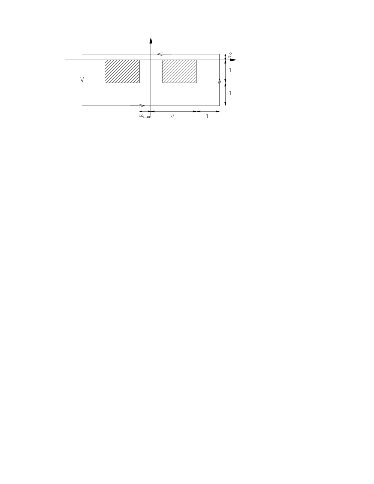
Figure 1: The integration path ${\Gamma_{\beta}}(c)$. If $c=\omega_{\text{max}}$, the shaded area contains all values of the type $\pm\omega(k)-{\rm i}\kappa$ for all $0\leq\kappa\leq 1$.

To apply the above Lemma we will choose the integration path $\Gamma$ as follows: For any $c>0$ and $0<\beta\leq 1$, let ${\Gamma_{\beta}}(c)$ denote the integration contour which follows the path shown in Fig. 1. Let ${\Gamma_{\beta}}={\Gamma_{\beta}}(\omega_{\text{max}})$, and we will choose $\Gamma={\Gamma_{\beta}}$ for some $\beta$. By construction, (4.55) then holds for all $w_{\ell}$ of the form $\pm\omega(k_{\ell})-{\rm i}\kappa_{\ell}$ with $k_{\ell}\in{\mathbb{T}}^{3}$ and $0\leq\kappa_{\ell}\leq 1$.

Lemma 4.10

Let $t>0$, $\kappa\geq 0$, and $N^{\prime},N_{1},N_{2}\in{\mathbb{N}}$ be given. Then for all $p\in{\mathbb{R}}^{3}$, and $f\in C^{\infty}({\mathbb{T}}^{3},{\mathbb{M}}_{2})$,

$${\mathbb{E}}\!\left[\left\langle G_{N^{\prime},N_{2}}(t;\varepsilon,\kappa)\psi^{\varepsilon}\!\left|B_{p,f}G_{N^{\prime},N_{1}}(t;\varepsilon,\kappa)\psi^{\varepsilon}\makebox[0.0pt]{$\displaystyle\phantom{G_{N^{\prime},N_{2}}(t;\varepsilon,\kappa)\psi^{\varepsilon}}$}\right.\!\right\rangle\right]$$

$$\quad=\sum_{S\in\pi(I)}\prod_{A\in S}C_{|A|}\,\mathcal{K}(t,S;(N^{\prime},N_{2}),(N^{\prime},N_{1}),\varepsilon,\kappa,p,f)$$ (4.57)

where $I=I_{N^{\prime}+N_{1},N^{\prime}+N_{2}}$, and for any partition $S\in\pi(I)$ we have defined

$$\mathcal{K}(t,S;(N^{\prime},N_{2}),(N^{\prime},N_{1}),\varepsilon,\kappa,p,f)$$

$$\quad=(-{\rm i})^{\bar{N}_{1}-\bar{N}_{2}}\varepsilon^{\bar{N}/2}\int_{{\mathbb{T}}^{3}}{\rm d}\eta_{0}\oint_{\Gamma_{\beta}}\frac{{\rm d}z}{2\pi}\oint_{\Gamma_{\beta}}\frac{{\rm d}z^{\prime}}{2\pi}\,{\rm e}^{-{\rm i}t(z+z^{\prime})}$$

$$\qquad\times\int_{({\mathbb{T}}^{3})^{\bar{N}+1}}\!{\rm d}\eta\,\delta(\eta_{\bar{N}_{1}+1}+p)\prod_{A\in S}\delta\Bigl{(}\sum_{\ell\in A}\eta_{\ell}\Bigr{)}\,\smash{\widehat{\psi}}^{\varepsilon}(\eta_{0}-p)\cdot$$

$$\quad\Bigl{[}\prod_{\ell=\bar{N}_{1}+3+N^{\prime}}^{\bar{N}+2}\Bigl{(}\frac{{\rm i}}{z^{\prime}+H(k_{\ell})}v(k_{\ell},k_{\ell-1})\Bigr{)}\prod_{\ell=\bar{N}_{1}+3}^{\bar{N}_{1}+2+N^{\prime}}\Bigl{(}\frac{{\rm i}}{z^{\prime}+{\rm i}\kappa+H(k_{\ell})}v(k_{\ell},k_{\ell-1})\Bigr{)}$$

$$\quad\times\frac{{\rm i}}{z^{\prime}+{\rm i}\kappa+H(k_{\bar{N}_{1}+2})}f\Bigl{(}k_{\bar{N}_{1}+1}-\frac{1}{2}p\Bigr{)}\frac{{\rm i}}{z+{\rm i}\kappa-H(k_{\bar{N}_{1}+1})}$$

$$\quad\times\prod_{\ell=N_{1}+1}^{N_{1}+N^{\prime}}\Bigl{(}v(k_{\ell+1},k_{\ell})\frac{{\rm i}}{z+{\rm i}\kappa-H(k_{\ell})}\Bigr{)}\prod_{\ell=1}^{N_{1}}\Bigl{(}v(k_{\ell+1},k_{\ell})\frac{{\rm i}}{z-H(k_{\ell})}\Bigr{)}\smash{\widehat{\psi}}^{\varepsilon}(\eta_{0})\Bigr{]}$$ (4.58)

with $\bar{N}_{i}=N_{i}+N^{\prime}$ for $i=1,2$, and $\bar{N}=\bar{N}_{1}+\bar{N}_{2}$. $H$ and $v$ are matrix-valued functions, $v$ is defined by (3.3) and $H(k)_{\sigma^{\prime}\sigma}=\delta_{\sigma^{\prime}\sigma}\sigma\omega(k)$. $0<\beta\leq 1$ is arbitrary, and ${\Gamma_{\beta}}$ denotes the corresponding integration path.

Proof.

First we use the definition of the two $G$-operators, (4.6), to express them as integrals over time-variables which we denote by $s$ and $s^{\prime}$. Since these are vector valued integrals, the scalar product can be taken inside the time-integrations. Then Fubini’s theorem allows swapping the order of the time-integrations and the expectation value. For this we need to have measurability with respect to the product measure, which can be proven by showing, as in (4.2), that the integrand is a limit of a sequence of measurable functions. We use Lemma 4.8 to express the remaining expectation value as an integral over the $\eta$-variables, and apply Fubini’s theorem to exchange the order of the $s$- and $s^{\prime}$-integrations and the $\eta$-integration. By Lemma 4.9:3 we can express the $s$ and $s^{\prime}$ -integrals as integrals over $z$ and $z^{\prime}$, and then summing over the $\sigma$-variables we arrive at the integrand in (4.10). The only remaining step is to reorder the $\eta$- and $z$-, $z^{\prime}$-integrals as given in (4.10) which is allowed by Fubini’s theorem. ∎

Corollary 4.11

$$F^{\varepsilon}_{\text{main}}(\bar{p},\bar{n},\bar{t})$$ (4.59)

$$\quad=\sum_{N_{1},N_{2}=0}^{N_{0}(\varepsilon)-1}\sum_{S\in\pi(I_{N_{1},N_{2}})}\prod_{A\in S}C_{|A|}\,\mathcal{K}(\bar{t}/\varepsilon,S;(0,N_{2}),(0,N_{1}),\varepsilon,0,\varepsilon\bar{p},e_{\bar{n}}P_{++}).$$

Proof.

By definition (4.32),

$$F^{\varepsilon}_{\text{main}}(\bar{p},\bar{n},\bar{t})=\sum_{N_{1},N_{2}=0}^{N_{0}(\varepsilon)-1} {\mathbb{E}}\!\left[\left\langle F_{N_{2}}(\bar{t}/\varepsilon;\varepsilon)\psi^{\varepsilon}\!\left|B_{\varepsilon p,e_{\bar{n}}P_{++}}F_{N_{1}}(\bar{t}/\varepsilon;\varepsilon)\psi^{\varepsilon}\makebox[0.0pt]{$\displaystyle\phantom{F_{N_{2}}(\bar{t}/\varepsilon;\varepsilon)\psi^{\varepsilon}}$}\right.\!\right\rangle\right]$$ (4.60)

which yields (4.59) by using first (4.11) and then Lemma 4.10. ∎

Lemma 4.12

Let $t,\kappa>0$, and $N^{\prime}_{0},N_{0}\in{\mathbb{N}}$, with $N_{0}\geq 1$ be given. Then

$${\mathbb{E}}\!\left[\|A_{N^{\prime}_{0},N_{0}}(t;\varepsilon,\kappa)\psi^{\varepsilon}\|^{2}\right]=\sum_{S\in\pi(I)}\prod_{A\in S}C_{|A|}\,\mathcal{K}^{(\text{amp})}(t,S;N^{\prime}_{0},N_{0},\varepsilon,\kappa)$$ (4.61)

where $I=I_{N,N}$ with $N=N^{\prime}_{0}+N_{0}$, and for any partition $S\in\pi(I)$,

$$\mathcal{K}^{(\text{amp})}(t,S;N^{\prime}_{0},N_{0},\varepsilon,\kappa)=\varepsilon^{N}\int_{{\mathbb{T}}^{3}}{\rm d}\eta_{0}\oint_{\Gamma_{\beta}}\frac{{\rm d}z}{2\pi}\oint_{\Gamma_{\beta}}\frac{{\rm d}z^{\prime}}{2\pi}{\rm e}^{-{\rm i}t(z+z^{\prime})}$$

$$\quad\times\int_{({\mathbb{T}}^{3})^{2N+1}}\!{\rm d}\eta\,\delta(\eta_{N+1})\prod_{A\in S}\delta\Bigl{(}\sum_{\ell\in A}\eta_{\ell}\Bigr{)}\,\smash{\widehat{\psi}}^{\varepsilon}(\eta_{0})\cdot$$

$$\quad\Bigl{[}\prod_{\ell=N+3+N^{\prime}_{0}}^{2N+2}\Bigl{(}\frac{{\rm i}}{z^{\prime}+H(k_{\ell})}v(k_{\ell},k_{\ell-1})\Bigr{)}\prod_{\ell=N+3}^{N+2+N^{\prime}_{0}}\Bigl{(}\frac{{\rm i}}{z^{\prime}+{\rm i}\kappa+H(k_{\ell})}v(k_{\ell},k_{\ell-1})\Bigr{)}$$

$$\quad\times\prod_{\ell=N_{0}+1}^{N_{0}+N^{\prime}_{0}}\Bigl{(}v(k_{\ell+1},k_{\ell})\frac{{\rm i}}{z+{\rm i}\kappa-H(k_{\ell})}\Bigr{)}\prod_{\ell=1}^{N_{0}}\Bigl{(}v(k_{\ell+1},k_{\ell})\frac{{\rm i}}{z-H(k_{\ell})}\Bigr{)}\smash{\widehat{\psi}}^{\varepsilon}(\eta_{0})\Bigr{]}$$ (4.62)

where the matrix-valued functions $H$ and $v$, and the path ${\Gamma_{\beta}}$ are defined as in Lemma 4.10 and $0<\beta\leq 1$ is arbitrary.

Proof.

By following the same steps as in the proof of Lemma 4.10. ∎

Figure 2: An example of a graph for $\mathcal{K}$ corresponding to $N_{1}=1$, $N_{2}=3$, $N^{\prime}=2$, and to a partition $S$ with $|S|=4$. We have also indicated how we chose to label the interaction vertices, and a few momenta belonging to the propagator lines. See the text for a description of the precise meaning of the different components of the graph.

$\mathcal{K}$ is called the amplitude of the partition, or graph, $S$. It will be helpful to think of the amplitudes in terms of planar graphs, where the structure of the graph encodes the inter-dependence of the momenta $k_{\ell}$, as imposed by the product of delta-functions $\prod_{A\in S}\delta(\sum_{\ell\in A}\eta_{\ell})$. The graph is constructed by starting from the left with a circle, denoting the rightmost $\smash{\widehat{\psi}}^{\varepsilon}$, and then representing the different factors in the matrix product (4.10), in the order they are acting, so that a solid line represents a term ${\rm i}/(z-H)$, a cross a term $v$, a dashed line a term ${\rm i}/(z+{\rm i}\kappa-H)$, until we reach the observable $f$, which will be denoted by a square. After this the same procedure is repeated, except now a solid line denotes ${\rm i}/(z^{\prime}+H)$ and a dashed line, ${\rm i}/(z^{\prime}+{\rm i}\kappa+H)$. The line terminates at a circled asterisk which corresponds to $(\smash{\widehat{\psi}}^{\varepsilon})^{*}$. Each of the fractionals is called a propagator, and a cross is called an interaction vertex. Finally, all interaction vertices belonging to the same cluster in the partition $S$ are joined by a dotted line. Fig. 2 gives an illustration of such a graph.

The graph for $\mathcal{K}^{(\text{amp})}$ is constructed similarly. As $\mathcal{K}^{(\text{amp})}$ is missing the propagators attached to the observable, it is called the amplitude of an amputated graph. We divide the graphs into the following categories:

Definition 4.13

Let $N^{\prime},N\geq 0$ be given, and let $S\in\pi(I_{N,N^{\prime}})$. We call the partition $S$ irrelevant if it contains a singlet, i.e., if there is $A\in S$ such that $|A|=1$. Otherwise, the partition $S$ is called relevant, and then it is

higher order,

if there is $A\in S$ such that $|A|>2$.

crossing,

if it is a pairing which contains two pairs crossing each other, i.e., there are $\{i_{1},i_{2}\}$, $\{j_{1},j_{2}\}\in S$ such that $i_{1}<j_{1}<i_{2}<j_{2}$.

nested,

if it is neither of the above, but there is a pairing $\{i_{1},i_{2}\}\in S$ which is completely on one side of the observable, but which is not a nearest neighbour pairing, i.e., such that $i_{1}+1<i_{2}$ and either $i_{1}\geq N+2$ or $i_{2}\leq N$.

simple,

otherwise.

It will turn out that only the simple partitions related to the main term contribute to the kinetic scaling limit. The proof that all other partitions can be neglected will rely on the following Lemmas whose proofs are the most involved part of the analysis and will be given in Sections 4.4 and 5. As before, we let here $E_{0}=\sup_{\varepsilon}\|\psi^{\varepsilon}\|^{2}$.

Lemma 4.14 (Basic A-estimate)

There are constants $c$ and $c^{\prime}$, which depend only on $\omega$, such that for any $t>0$, $\kappa,\varepsilon\in(0,\frac{1}{2}]$, $N_{0},N_{0}^{\prime}\in{\mathbb{N}}$ with $N_{0}\geq 1$, and a relevant $S\in\pi(I_{N,N})$,

$$\left|\mathcal{K}^{(\text{amp})}(t,S;N^{\prime}_{0},N_{0},\varepsilon,\kappa)\right|\leq c^{\prime}E_{0}\,\varepsilon^{N-|S|}\Bigl{(}\frac{\varepsilon}{\kappa}\Bigr{)}^{n_{S}}\left(c\langle\varepsilon t\rangle\right)^{N}\Bigl{\langle}\ln\frac{\langle\varepsilon t\rangle}{\varepsilon}\Bigr{\rangle}^{2N}$$ (4.63)

where $N=N^{\prime}_{0}+N_{0}$ and

$$n_{S}=\left|\left\{\max A\left|\,A\in S\makebox[0.0pt]{$\displaystyle\phantom{\max A}$}\right.\!\right\}\cap\{N_{0},\ldots,N_{0}+1+2N^{\prime}_{0}\}\right|.$$ (4.64)

This estimate suffices to prove the bound for the amputated expectation value.

• Proof of Proposition 4.7: Let $\kappa=\kappa(\varepsilon)$ and $N^{\prime}_{0}=8N_{0}$ as in Definition 4.4, and denote $N=N_{0}+N^{\prime}_{0}=9N_{0}$. Let also $a=2\bar{\xi}(3\bar{\xi}^{2}+1)$ as in Lemma C.4, and assume that $\varepsilon_{1}\leq\min(1/a^{2},1/2)$ is chosen so that $\kappa(\varepsilon)\leq 1/2$ for all $\varepsilon\leq\varepsilon_{1}$. We then consider an arbitrary $\varepsilon\leq\varepsilon_{1}$.

  We can then apply Lemma 4.14, together with $\langle\varepsilon t\rangle\leq\langle\bar{t}\rangle=T$, arriving at

  $$\left|\mathcal{K}^{(\text{amp})}(t,S;N^{\prime}_{0},N_{0},\varepsilon,\kappa)\right|\leq c^{\prime}E_{0}\,\varepsilon^{N-|S|}\Bigl{(}\frac{\varepsilon}{\kappa}\Bigr{)}^{n_{S}}(cT)^{N}\Bigl{\langle}\ln\frac{T}{\varepsilon}\Bigr{\rangle}^{2N}.$$ (4.65)

  We still need to estimate the sum over the partitions $S$. First we sum over all partitions containing a cluster of size at least $7$. In this case, we estimate $\varepsilon/\kappa\leq 1$ and, using $\sqrt{\varepsilon}\leq 1/a$, apply Lemma C.4 which proves

  $$\sum_{\begin{subarray}{c}S\in\pi(I_{N,N}),\\ \exists A\in S:|A|>6\end{subarray}}\prod_{A\in S}\left|C_{|A|}\right|\,\left|\mathcal{K}^{(\text{amp})}(t,S;N^{\prime}_{0},N_{0},\varepsilon,\kappa)\right|$$

  $$\qquad\leq c^{\prime}E_{0}(cT)^{N}\Bigl{\langle}\ln\frac{T}{\varepsilon}\Bigr{\rangle}^{2N}(2N)!\,a^{6}\varepsilon^{3}.$$ (4.66)

  Let then $S$ be such that for all $A\in S$, $|A|\leq 6$. Then $|S|\geq(2N)/6=3N_{0}$, and thus $n_{S}\geq|S|-2N_{0}\geq N_{0}$. Therefore, $(\varepsilon/\kappa)^{n_{S}}\leq(\varepsilon/\kappa)^{N_{0}}$. To estimate the remaining sum over the partitions, we can neglect the restriction on the size of the clusters. We use Lemma C.4 to bound the sum over higher-order partitions, and compute the estimate for pairings explicitly. Since the number of possible pairings is $(2N)!/(2^{N}N!)\leq(2N)!$ we get

  $$\sum_{S\in\pi(I_{N,N})}\prod_{A\in S}\left|C_{|A|}\right|\,\varepsilon^{N-|S|}\leq(2N)!(1+\varepsilon a^{2})\leq 2(2N)!.$$ (4.67)

  We have thus proven that

  $$\sum_{S\in\pi(I_{N,N})}\prod_{A\in S}\left|C_{|A|}\right|\,\left|\mathcal{K}^{(\text{amp})}(t,S;N^{\prime}_{0},N_{0},\varepsilon,\kappa)\right|$$

  $$\qquad\leq c^{\prime}E_{0}(cT)^{N}\Bigl{\langle}\ln\frac{T}{\varepsilon}\Bigr{\rangle}^{2N}(2N)!\left(a^{6}\varepsilon^{3}+2\Bigl{(}\frac{\varepsilon}{\kappa}\Bigr{)}^{N_{0}}\right)$$ (4.68)

  from which (4.39) follows by Lemma 4.12 after redefinition of the constant $c^{\prime}$. The bound is trivially valid for $t=0$ since $\|A_{N^{\prime}_{0},N_{0}}(t)\|=0$. $\Box$

For the other estimates, we no longer need the additional decay provided by the terms containing $\kappa$. We do however need to make sure that its presence does not spoil any of the estimates for $G$. In the following Lemmas, whose proofs will be postponed until Section 4.4, $N^{\prime},N_{1},N_{2}\geq 0$ and $N_{0}\geq 1$, and we use the notations $\bar{N}_{1}=N^{\prime}+N_{1}$, $\bar{N}_{2}=N^{\prime}+N_{2}$, $\bar{N}=\bar{N}_{1}+\bar{N}_{2}$. Let also $I=I_{\bar{N}_{1},\bar{N}_{2}}$.

Lemma 4.15 (Basic estimate)

There are constants $c$ and $c^{\prime}$, which depend only on $\omega$, such that for any $t>0$, $\kappa,\varepsilon\in(0,\frac{1}{2}]$, and every relevant $S\in\pi(I)$,

$$\left|\mathcal{K}(t,S;(N^{\prime},N_{2}),(N^{\prime},N_{1}),\varepsilon,\kappa,p,f)\right|$$

$$\quad\leq c^{\prime}\|f\|_{\infty}E_{0}\left(c\varepsilon\langle t\rangle\right)^{\!\frac{\bar{N}}{2}}\Bigl{\langle}\ln\frac{\langle\varepsilon t\rangle}{\varepsilon}\Bigr{\rangle}^{\bar{N}+2}\varepsilon^{\mathbbm{1}(\bar{N}>0)(\bar{N}-2|S|)/2}.$$ (4.69)

Lemma 4.16 (Crossing partition)

Let the assumptions of Lemma 4.15 be satisfied. There is a constant $c^{\prime\prime}$, depending only on $\omega$, such that if $S\in\pi(I)$ is crossing, then the bound on the right hand side of (4.15) is valid also if it is multiplied by

$$c^{\prime\prime}\langle t\rangle^{-\gamma}\Bigl{\langle}\ln\frac{\langle\varepsilon t\rangle}{\varepsilon}\Bigr{\rangle}^{\max(0,d_{2}-2)},$$ (4.70)

where $\gamma$ and $d_{2}$ are as in the assumption (DR4).

Lemma 4.17 (Nested partition)

Let the assumptions of Lemma 4.15 be satisfied. There are constants $c^{\prime\prime}_{1}$, $c^{\prime\prime}_{2}$, depending only on $\omega$, such that if $S\in\pi(I)$ is nested, then the bound on the right hand side of (4.15) is valid also if it is multiplied by

$$c^{\prime\prime}_{1}(c^{\prime\prime}_{2})^{\frac{\bar{N}}{2}}\bar{N}^{d_{1}}\!\langle t\rangle^{-\frac{1}{2}}.$$ (4.71)

These immediately yield the following estimate for the contribution from non-simple partitions:

Corollary 4.18

There are constants $c$ and $c^{\prime}$ and $\varepsilon^{\prime}$, which depend only on $\omega$ and $\bar{\xi}$, such that, if $0<\varepsilon\leq\varepsilon^{\prime}$, $0\leq\kappa\leq 1/2$, $t>0$, and $\bar{N}>0$, then

$$\sum_{\begin{subarray}{c}S\in\pi(I),\\ S\text{ not simple}\end{subarray}}\prod_{A\in S}|C_{|A|}|\,|\mathcal{K}(t,S;(N^{\prime},N_{2}),(N^{\prime},N_{1}),\varepsilon,\kappa,p,f)|$$

$$\quad\leq c^{\prime}\|f\|_{\infty}E_{0}\left(c\varepsilon\langle t\rangle\right)^{\!\frac{\bar{N}}{2}}\bar{N}!\Bigl{\langle}\ln\frac{\langle\varepsilon t\rangle}{\varepsilon}\Bigr{\rangle}^{\bar{N}+\max(2,d_{2})}\bar{N}^{d_{1}}\Bigl{(}\frac{\langle\varepsilon t\rangle}{\langle t\rangle}\Bigr{)}^{\gamma^{\prime}}$$ (4.72)

where $\gamma^{\prime}$ is defined in (4.24), and $d_{1},d_{2}$ are the constants in (DR3) and (DR4).

Proof.

Let $a=2\bar{\xi}(3\bar{\xi}^{2}+1)$ as in Lemma C.4, and let $\varepsilon^{\prime}=\min(1/a^{2},1/2)$. Then for any $0<\varepsilon\leq\varepsilon^{\prime}$, we get from Lemmas 4.15 and C.4,

$$\sum_{\begin{subarray}{c}S\in\pi(I),\\ \exists A\in S:|A|>2\end{subarray}}\prod_{A\in S}\left|C_{|A|}\right|\,\left|\mathcal{K}(t,S;(N^{\prime},N_{2}),(N^{\prime},N_{1}),\varepsilon,\kappa,p,f)\right|$$

$$\qquad\leq c^{\prime}\|f\|_{\infty}E_{0}\left(c\varepsilon\langle t\rangle\right)^{\!\frac{\bar{N}}{2}}\Bigl{\langle}\ln\frac{\langle t\rangle}{\varepsilon}\Bigr{\rangle}^{\bar{N}+2}\bar{N}!\langle a\rangle^{2}\sqrt{\varepsilon}.$$ (4.73)

There are at most $\bar{N}!$ pairings, which can be combined with Lemmas 4.16 and 4.17 to prove (4.18) after redefinition of constants. ∎

Figure 3: An example of a simple graph $S_{m}(n,n^{\prime})$ with $\kappa=0$, $m=2$, and $n=(1,2,0)$, $n^{\prime}=(0,0,1)$. We have also depicted the dependence of the momenta outside the gates, see Sec. 5.1 for details.

We need one more estimate before we can complete the proof of Proposition 4.6.

Lemma 4.19 (Simple partition)

For any $m\in{\mathbb{N}}$ and $n,n^{\prime}\in{\mathbb{N}}^{m+1}$, let $S_{m}(n^{\prime},n)$ denote the partition which consists a ladder of $m$ “rungs” and where the components of $n$ and $n^{\prime}$ define the number of “gates” between the rungs, see Fig. 3.

$S\in\pi(I_{\bar{N}_{1},\bar{N}_{2}})$ is simple if and only if there are $m$ and $n,n^{\prime}$, with $m+2\sum_{j=1}^{m+1}n_{j}=\bar{N}_{1}$ and $m+2\sum_{j=1}^{m+1}n^{\prime}_{j}=\bar{N}_{2}$, such that $S=S_{m}(n,n^{\prime})$. In addition, there are constants $c$, $c^{\prime}$, and $c_{i}$, $i=0,1,2,3$, depending only on $\omega$, such that for any $t>0$, $\kappa,\varepsilon\in(0,\frac{1}{2}]$,

$$\left|\mathcal{K}(t,S_{m}(n,n^{\prime});(N^{\prime},N_{2}),(N^{\prime},N_{1}),\varepsilon,\kappa,p,f)\right|$$

$$\quad\leq\frac{E_{0}\|f\|_{\infty}(c\varepsilon t)^{\bar{N}/2}}{[((\bar{N}_{1}+m)/2)!((\bar{N}_{2}+m)/2)!]^{1/2}}+c^{\prime}\|f\|_{\infty}E_{0}(c_{0}\varepsilon\langle t\rangle)^{\bar{N}/2}$$

$$\quad\times\Bigl{\langle}\ln\frac{\langle\varepsilon t\rangle}{\varepsilon}\Bigr{\rangle}^{3}(\bar{N}+1)\Bigl{(}1+c_{1}\frac{|p|}{\sqrt{\varepsilon}}+c_{2}\frac{\kappa}{\varepsilon}+c_{3}\sqrt{1+\kappa/\varepsilon}\Bigr{)}\frac{\langle\varepsilon t\rangle}{\langle t\rangle^{1/2}}.$$ (4.74)

• Proof of Proposition 4.6: Let $\kappa=\kappa(\varepsilon)$ and $N^{\prime}_{0}=8N_{0}$ as in Definition 4.4. Let also $a=2\bar{\xi}(3\bar{\xi}^{2}+1)$ as in Lemma C.4, and assume that $\varepsilon_{1}\leq\min(1/a^{2},1/2)$ is chosen so that $\kappa(\varepsilon)\leq 1/2$ for all $\varepsilon\leq\varepsilon_{1}$. We then consider an arbitrary $0<\varepsilon\leq\varepsilon_{1}$, $0\leq N^{\prime}<N^{\prime}_{0}$ and $0<t\leq\bar{t}/\varepsilon$.

  By Lemma 4.10, ${\mathbb{E}}\!\left[\|G_{N^{\prime}\!,N_{0}}(t;\varepsilon,\kappa)\psi^{\varepsilon}\|^{2}\right]$ is bounded by

  $$\sum_{S\in\pi(I)}\prod_{A\in S}\left|C_{|A|}\right|\,|\mathcal{K}(t,S;(N^{\prime},N_{0}),(N^{\prime},N_{0}),\varepsilon,\kappa(\varepsilon),0,\mathbbm{1})|$$ (4.75)

  where $I=I_{N_{1},N_{1}}$ with $N_{1}=N^{\prime}+N_{0}$. Let also $\bar{N}=2(N^{\prime}+N_{0})$ when $1<\bar{N}\leq 18N_{0}$. $\varepsilon$ is small enough for applying Corollary 4.18 and Lemma 4.19, yielding an upper bound

  $$c^{\prime}E_{0}\left(c\varepsilon\langle t\rangle\right)^{\!\frac{\bar{N}}{2}}\bar{N}!\Bigl{\langle}\ln\frac{\langle\varepsilon t\rangle}{\varepsilon}\Bigr{\rangle}^{\bar{N}+\max(2,d_{2})}\bar{N}^{d_{1}}\Bigl{(}\frac{\langle\varepsilon t\rangle}{\langle t\rangle}\Bigr{)}^{\gamma^{\prime}}$$

  $$\quad+c^{\prime\prime}E_{0}(c_{0}^{\prime}\varepsilon\langle t\rangle)^{\!\frac{\bar{N}}{2}}(\bar{N}+1)!\Bigl{\langle}\ln\frac{\langle\varepsilon t\rangle}{\varepsilon}\Bigr{\rangle}^{3}\langle\ln\varepsilon\rangle^{b_{0}}\frac{\langle\varepsilon t\rangle}{\langle t\rangle^{1/2}}$$

  $$\quad+E_{0}\sum_{S_{m}(n,n^{\prime})\in\pi(I)}\frac{(c_{0}\varepsilon t)^{\bar{N}/2}}{((N_{1}+m)/2)!}$$ (4.76)

  where we have estimated the number of simple pairings by $\bar{N}!$ and used the explicit form of $\kappa(\varepsilon)$. Now, if $0<\varepsilon_{1}\leq\varepsilon^{\prime}$ is such that $N_{0}(\varepsilon)\geq b_{0}+1$ for all $0<\varepsilon\leq\varepsilon_{1}$, then for these $\varepsilon$, the sum of the first two terms is bounded by

  $$c^{\prime\prime\prime}E_{0}\left(c^{\prime\prime}_{0}\varepsilon\langle t\rangle\right)^{\!\frac{\bar{N}}{2}}\bar{N}!\Bigl{\langle}\ln\frac{\langle\varepsilon t\rangle}{\varepsilon}\Bigr{\rangle}^{\bar{N}+\max(2,d_{2})}\bar{N}^{\max(1,d_{1})}\frac{\langle\varepsilon t\rangle}{\langle t\rangle^{\gamma^{\prime}}}$$

  $$\quad\leq c^{\prime\prime\prime}E_{0}\left(c^{\prime\prime}_{0}\varepsilon\langle\bar{t}/\varepsilon\rangle\right)^{\!\frac{\bar{N}}{2}}\bar{N}!\Bigl{\langle}\ln\frac{\langle\bar{t}\rangle}{\varepsilon}\Bigr{\rangle}^{\bar{N}+\max(2,d_{2})}\bar{N}^{\max(1,d_{1})}\frac{\langle\bar{t}\rangle}{\langle\bar{t}/\varepsilon\rangle^{\gamma^{\prime}}}$$ (4.77)

  where we have used $\bar{N}>1\geq 2\gamma^{\prime}$ to justify the estimate $\langle t\rangle^{\bar{N}/2-\gamma^{\prime}}\leq\langle\bar{t}/\varepsilon\rangle^{\bar{N}/2-\gamma^{\prime}}$. Here applying first $\varepsilon\langle\bar{t}/\varepsilon\rangle\leq\langle\bar{t}\rangle=T$ and then $\bar{N}\leq 18N_{0}$ yields the first term in (4.6).

  We estimate the last term in ( ‣ 4.2) using

  $$\sum_{S_{m}(n,n^{\prime})\in\pi(I)}\frac{2^{-\bar{N}/2}}{((N_{1}+m)/2)!}\leq\sum_{m=0}^{N_{1}}\sum_{n\in{\mathbb{N}}^{m+1}}\sum_{n^{\prime}\in{\mathbb{N}}^{m+1}}\frac{1}{((N_{1}+m)/2)!}$$

  $$\qquad\mathbbm{1}\Bigl{(}N_{1}=m+2\sum_{j=1}^{m+1}n_{j}\Bigr{)}\mathbbm{1}\Bigl{(}N_{1}=m+2\sum_{j=1}^{m+1}n^{\prime}_{j}\Bigr{)}\frac{1}{2^{m}}\prod_{j=0}^{m}\Bigl{(}\frac{1}{2^{n_{j}}}\frac{1}{2^{n^{\prime}_{j}}}\Bigr{)}$$

  $$\quad\leq\frac{1}{\lfloor N_{1}/2\rfloor!}\sum_{m=0}^{\infty}2^{m+2}\frac{1}{\lfloor m/2\rfloor!}$$ (4.78)

  where the sum over $m$ is finite. Applying $N_{1}\geq N_{0}$ and $2c_{0}\varepsilon t\leq\langle 2c_{0}\rangle T$, and readjusting the constants finishes then the proof of the Proposition. $\Box$

4.3 Consequences of dispersivity

In the derivation of the above Lemmas, we will heavily rely on the following estimates, which follow from the assumed sufficiently strong dispersivity of $\omega$.

Lemma 4.20

Let $\omega\in L^{\infty}({\mathbb{T}}^{3})$ be such that it satisfies the assumption (DR3) with a constant $c_{\omega}$, and assume that $\omega_{\text{max}}=\sup_{k}|\omega(k)|<\infty$. Then, for any $\kappa\geq 0$ and $\beta>0$ such that $\kappa+\beta\leq 1$, all of the following propositions hold for ${\Gamma_{\beta}}={\Gamma_{\beta}}(\omega_{\text{max}})$ and $n\in{\mathbb{N}}$:

1. $\displaystyle\sup_{\sigma=\pm 1,k\in{\mathbb{T}}^{3},z\in{\Gamma_{\beta}}}\frac{1}{|z+{\rm i}\kappa-\sigma\omega(k)|}\leq\frac{1}{\beta+\kappa}$,

2. $\displaystyle\sup_{\sigma=\pm 1,k\in{\mathbb{T}}^{3}}\oint_{{\Gamma_{\beta}}}\frac{|{\rm d}z|}{2\pi}\frac{1}{|z+{\rm i}\kappa-\sigma\omega(k)|}\leq|{\Gamma_{\beta}}|\langle\ln(\beta+\kappa)\rangle$.

3. $\displaystyle\sup_{\sigma=\pm 1,z\in{\Gamma_{\beta}}}\int_{{\mathbb{T}}^{3}}{\rm d}k\,\frac{1}{|z+{\rm i}\kappa-\sigma\omega(k)|}\leq 12c_{\omega}\langle\ln(\beta+\kappa)\rangle$.

4. For all $n\geq 2$, $\displaystyle\sup_{\sigma=\pm 1,z\in{\Gamma_{\beta}}}\int_{{\mathbb{T}}^{3}}{\rm d}k\,\frac{1}{|z+{\rm i}\kappa-\sigma\omega(k)|^{n}}\leq\frac{3c_{\omega}}{(\beta+\kappa)^{n-1}}$.

5. For any smooth function $f$,

   $$\sup_{\sigma=\pm 1,z\in{\Gamma_{\beta}}}\left|\int_{{\mathbb{T}}^{3}}{\rm d}k\,\frac{f(k)}{z+{\rm i}\kappa-\sigma\omega(k)}\right|\leq 3c_{\omega}\|f\|_{d_{1},\infty},$$ (4.79)

   and for all $n\geq 2$, and $n_{1},n_{2}\geq 0$ such that $n_{1}+n_{2}=n$,

   $$\sup_{\sigma=\pm 1,z\in{\Gamma_{\beta}}}\left|\int_{{\mathbb{T}}^{3}}{\rm d}k\,\frac{f(k)}{(z-\sigma\omega(k))^{n_{1}}(z+{\rm i}\kappa-\sigma\omega(k))^{n_{2}}}\right|\leq\frac{3c_{\omega}\|f\|_{d_{1},\infty}}{\beta^{n-3/2}}.$$ (4.80)

These results are similar to those used in [3, 6, 7], as are the ideas behind the proofs. However, we present here a more straightforward way of doing the analysis. The main additional ingredient we need is the following Lemma:

Lemma 4.21

For any $r\in{\mathbb{R}}$ and $0<\beta\leq 1$,

$$\frac{1}{\sqrt{r^{2}+\beta^{2}}}=\int_{-\infty}^{\infty}\!\!{\rm d}s\,{\rm e}^{{\rm i}sr}\int_{0}^{\infty}\!\frac{{\rm d}x}{\pi}\frac{1}{\sqrt{1+x^{2}}}{\rm e}^{-\beta|s|\sqrt{1+x^{2}}}$$ (4.81)

where for any $s\in{\mathbb{R}}$, $s\neq 0$,

$$\int_{0}^{\infty}\!\frac{{\rm d}x}{\pi}\frac{1}{\sqrt{1+x^{2}}}{\rm e}^{-\beta|s|\sqrt{1+x^{2}}}\leq\langle\ln\beta\rangle{\rm e}^{-\beta|s|}+\mathbbm{1}(|s|\leq 1)\ln|s|^{-1}$$ (4.82)

and the function on the right hand side belongs to $L^{1}({\rm d}s)$.

Proof.

Suppose we have proven the bound in (4.82). Since $\int_{-1}^{1}{\rm d}s\ln|s|^{-1}=2$, the bound on the right hand side belongs to $L^{1}({\rm d}s)$, and we can apply Fubini’s theorem in (4.81) to swap the $s$ and $x$ integrals. Then

$$\int_{-\infty}^{\infty}\!\!{\rm d}s\,{\rm e}^{{\rm i}sr-\beta\sqrt{1+x^{2}}|s|}=\frac{2\beta\sqrt{1+x^{2}}}{\beta^{2}(1+x^{2})+r^{2}}$$ (4.83)

from which (4.81) follows immediately.

We thus only need to prove the bound (4.82). Let first $0<|s|\leq 1$. Then $\beta|s|\leq 1$, and

$$\int_{0}^{\infty}\!\frac{{\rm d}x}{\sqrt{1+x^{2}}}{\rm e}^{-\beta|s|\sqrt{1+x^{2}}}\leq\int_{0}^{(\beta|s|)^{-1}}\!\!\!\frac{{\rm d}x}{\sqrt{1+x^{2}}}{\rm e}^{-\beta|s|}+\int_{(\beta|s|)^{-1}}^{\infty}\!\!{\rm d}x\,\beta|s|{\rm e}^{-\beta|s|x}$$

$$\quad={\rm arsinh}((\beta|s|)^{-1}){\rm e}^{-\beta|s|}+{\rm e}^{-1}\leq(2+\ln\beta^{-1}){\rm e}^{-\beta|s|}+\ln|s|^{-1}$$

$$\quad\leq 2\sqrt{2}\langle\ln\beta\rangle{\rm e}^{-\beta|s|}+\ln|s|^{-1}\leq\pi(\langle\ln\beta\rangle{\rm e}^{-\beta|s|}+\ln|s|^{-1})$$ (4.84)

where we used the fact that for all $x\geq 1$

$${\rm arsinh}\,x=\ln(x+\sqrt{x^{2}+1})\leq 1+\ln x.$$ (4.85)

If $|s|\geq 1$, similarly

$$\int_{0}^{\infty}\!\!\frac{{\rm d}x}{\sqrt{1+x^{2}}}{\rm e}^{-\beta|s|\sqrt{1+x^{2}}}\leq\int_{0}^{1/\beta}\!\!\frac{{\rm d}x}{\sqrt{1+x^{2}}}{\rm e}^{-\beta|s|}+\int_{1/\beta}^{\infty}\!\!{\rm d}x\,\beta{\rm e}^{-\beta|s|x}$$

$$\quad={\rm arsinh}(1/\beta){\rm e}^{-\beta|s|}+{\rm e}^{-|s|}\leq(2+\ln\beta^{-1}){\rm e}^{-\beta|s|}\leq\pi\langle\ln\beta\rangle{\rm e}^{-\beta|s|}$$ (4.86)

which completes the proof of inequality (4.82). ∎

• Proof of Lemma 4.20: The integration path ${\Gamma_{\beta}}$ consists of two pieces: the uppermost part parameterized by $[-1-\omega_{\text{max}},\omega_{\text{max}}+1]\ni\alpha\mapsto z=-\alpha+{\rm i}\beta$, and the remainder whose distance from the set $\left\{|{\rm Re\,}z|\leq\omega_{\text{max}}\left|\,-1\leq{\rm Im\,}z\leq 0\makebox[0.0pt]{$\displaystyle\phantom{|{\rm Re\,}z|\leq\omega_{\text{max}}}$}\right.\!\right\}$ is at least $1$, see Fig. 1. Therefore, on the first part $|z+{\rm i}\kappa-\sigma\omega(k)|$ is bounded from below by $\beta+\kappa\leq 1$, and on the second part by $1$. This proves item 1.

  For item 2, we first separate a segment of length two in the uppermost part of ${\Gamma_{\beta}}$, corresponding to $|\alpha-\sigma\omega(k)|\leq 1$. The integral over the remaining part is then bounded by $(|{\Gamma_{\beta}}|-2)/(2\pi)$. The value of the integral over the segment is equal to $1/\pi$ times

  $$\int_{0}^{1}\!{\rm d}r\,\frac{1}{\sqrt{r^{2}+(\beta+\kappa)^{2}}}=\Bigl{/}_{\!\!\!0}^{1}\,\ln(r+\sqrt{(\beta+\kappa)^{2}+r^{2}})\leq 1+|\ln(\beta+\kappa)|.$$ (4.87)

  Thus the total integral is bounded by

  $$\frac{|{\Gamma_{\beta}}|+2|\ln(\beta+\kappa)|}{2\pi}\leq|{\Gamma_{\beta}}|\frac{1+|\ln(\beta+\kappa)|}{2\pi}\leq|{\Gamma_{\beta}}|\langle\ln(\beta+\kappa)\rangle.$$ (4.88)

  In all of the estimates in items 3–5 it is sufficient to assume that $z$ belongs to the uppermost part of the integration path, i.e., $z=\alpha+{\rm i}\beta$ for some $\alpha\in{\mathbb{R}}$, since otherwise we trivially have bounds by $1$ for items 3 and 4, and by $\|f\|_{\infty}$ for item 5. Let us also denote $\beta^{\prime}=\beta+\kappa$. Then in item 3, the bound follows from applying Lemma 4.21, the assumption (DR3), and the relations

  $$\int_{0}^{1}\!{\rm d}s\,\ln|s|^{-1}=1\qquad\text{and}\qquad\int_{0}^{\infty}\!{\rm d}s\,\frac{1}{\langle s\rangle^{3/2}}\leq 1+\int_{1}^{\infty}\!{\rm d}s\,s^{-3/2}=3.$$ (4.89)

  For item 4, we first use the trivial bound in item 2 to see that the integrand is bounded by $(\beta^{\prime})^{2-n}/|\alpha-\sigma\omega(k)+{\rm i}\beta^{\prime}|^{2}$. Then the estimate follows from applying the equality

  $$\frac{1}{r^{2}+(\beta^{\prime})^{2}}=\frac{1}{2\beta^{\prime}}\int_{-\infty}^{\infty}\!\!{\rm d}s\,{\rm e}^{{\rm i}sr-\beta^{\prime}|s|}$$ (4.90)

  valid for all $r\in{\mathbb{R}}$, and then estimating the result using the assumption (DR3).

  Finally, for item 5, we use the fact that in all of the terms the imaginary part is strictly positive, proving

  $$\int_{{\mathbb{T}}^{3}}{\rm d}k\,\frac{f(k)}{(\alpha+{\rm i}\beta-\sigma\omega(k))^{n_{1}}(\alpha+{\rm i}(\beta+\kappa)-\sigma\omega(k))^{n_{2}}}$$

  $$\quad=(-{\rm i})^{n}\int_{{\mathbb{R}}_{+}^{n}}\!{\rm d}s\,{\rm e}^{-\sum_{\ell=1}^{n_{2}}s_{\ell}\kappa}{\rm e}^{-(\beta-{\rm i}\alpha)\sum_{\ell=1}^{n}s_{\ell}}\int_{{\mathbb{T}}^{3}}{\rm d}k\,f(k){\rm e}^{-{\rm i}\sigma\omega(k)\sum_{\ell=1}^{n}s_{\ell}}.$$ (4.91)

  By (DR3), this is bounded by

  $$\int_{{\mathbb{R}}_{+}^{n}}\!{\rm d}s\,{\rm e}^{-\beta\sum_{\ell}s_{\ell}}\frac{c_{\omega}}{\Bigl{\langle}\sum_{\ell}s_{\ell}\Bigr{\rangle}^{3/2}}\|f\|_{d_{1},\infty}=\frac{c_{\omega}\|f\|_{d_{1},\infty}}{(n-1)!}\int_{0}^{\infty}\!{\rm d}s\frac{s^{n-1}}{\langle s\rangle^{3/2}}{\rm e}^{-\beta s}.$$ (4.92)

  If $n=1$, the integral over $s$ is bounded by $3$. Otherwise, it is bounded by

  $$1+\int_{1}^{\infty}\!{\rm d}s\,s^{n-1-3/2}{\rm e}^{-\beta s}\leq 1+\beta^{3/2-n}\left(1+\int_{0}^{\infty}\!{\rm d}r\,r^{n-2}{\rm e}^{-r}\right)$$

  $$\leq 3\beta^{3/2-n}(n-1)!$$ (4.93)

  where we have used $\beta\leq 1$. This finishes the proof of item 5. $\Box$

Corollary 4.22

Under the same assumptions as in Lemma 4.20, for both $\sigma=\pm 1$,

1. $\displaystyle\sup_{k\in{\mathbb{T}}^{3},z\in{\Gamma_{\beta}}}\Bigl{\|}\frac{1}{z+{\rm i}\kappa-\sigma H(k)}\Bigr{\|}\leq\frac{1}{\beta+\kappa}$,

2. $\displaystyle\sup_{k\in{\mathbb{T}}^{3}}\oint_{{\Gamma_{\beta}}}\frac{|{\rm d}z|}{2\pi}\Bigl{\|}\frac{1}{z+{\rm i}\kappa-\sigma H(k)}\Bigr{\|}\leq 2|{\Gamma_{\beta}}|\langle\ln\beta\rangle$.

3. $\displaystyle\sup_{z\in{\Gamma_{\beta}}}\int_{{\mathbb{T}}^{3}}{\rm d}k\,\Bigl{\|}\frac{1}{z+{\rm i}\kappa-\sigma H(k)}\Bigr{\|}\leq 24c_{\omega}\langle\ln\beta\rangle$.

Proof.

Item 1 is clear. The other two follow by first estimating the integrands by

$$\Bigl{\|}\frac{1}{z+{\rm i}\kappa-\sigma H(k)}\Bigr{\|}\leq\sum_{\sigma^{\prime}=\pm 1}\Bigl{|}\frac{1}{z+{\rm i}\kappa-\sigma^{\prime}\omega(k)}\Bigr{|}$$ (4.94)

and then applying the Lemma. ∎

4.4 Derivation of the basic bounds

Let us now fix the way of resolving the momentum delta-functions. Given a partition $S\in\pi(I_{N,N^{\prime}})$, we define $M(S)=\left\{\max A\left|\,A\in S\makebox[0.0pt]{$\displaystyle\phantom{\max A}$}\right.\!\right\}$, and for any index $\ell\in I_{N,N^{\prime}}$, let $A(\ell)$ denote the unique cluster in $S$ which contains $\ell$. For each $A\in S$ we integrate out $\eta_{\ell}$ with $\ell=\max A$. Then every $\eta_{\ell}$ with $\ell\in I_{N,N^{\prime}}\!\setminus M(S)$ is free, i.e., it is integrated over the whole of ${\mathbb{T}}^{3}$ independently of the values of the other integration variables, and for $\ell\in M(S)$ we have

$$\eta_{\ell}=-\sum_{n\in A(\ell):n<\ell}\eta_{n}.$$ (4.95)

Given a propagator index $\ell\in\{1,\ldots,N+N^{\prime}+2\}$, we call a cluster $A\in S$ broken at $\ell$ if $\min A<\ell\leq\max A$, and we call an index $n\in I_{N,N^{\prime}}$ free at $\ell$ if $n<\ell$ and $\max A(n)\geq\ell$. The first terminology is explained by Figure 2, and the second comes from the fact that the function $k_{\ell}(\eta)$ depends only on those free integration variables $\eta_{n}$ which are free at $\ell$. Explicitly, by (4.42) we have for all $\ell$

$$k_{\ell}(\eta)=\eta_{0}+\mathbbm{1}(\ell>N+1)\eta_{N+1}+\sum_{\begin{subarray}{c}n\in I_{N,N^{\prime}}:n<\ell\\ \max A(n)\geq\ell\end{subarray}}\eta_{n}.$$ (4.96)

The following Lemma will allow estimating most of the $\eta$-integrals:

Lemma 4.23

Let $N^{\prime},N\in{\mathbb{N}}$ be given, and assume $S\in\pi(I_{N,N^{\prime}})$. Define $M^{\prime}=M(S)\cup\{N+1\}$, and for each $\ell=2,\ldots,N+N^{\prime}+1$ let $f_{\ell}\in L^{1}({\mathbb{T}}^{3})\cap L^{\infty}({\mathbb{T}}^{3})$ with $f_{\ell}\geq 0$. Then, if $n\in\{1,\ldots,N+N^{\prime}\}$ is such that $|I_{n}\!\setminus M^{\prime}|>1$, we have for $n^{\prime}=\max(I_{n}\!\setminus M^{\prime})-1$

$$\int_{({\mathbb{T}}^{3})^{I_{n}\!\setminus M^{\prime}}}\!\!\!\!\!{\rm d}\eta\,\prod_{\ell=2}^{n+1}f_{\ell}(k_{\ell}(\eta))\leq\|f_{n^{\prime}+2}\|_{1}\prod_{\ell=n^{\prime}+3}^{n+1}\|f_{\ell}\|_{\infty}\int_{({\mathbb{T}}^{3})^{I_{n^{\prime}}\!\setminus M^{\prime}}}\!\!\!\!{\rm d}\eta\,\prod_{\ell=2}^{n^{\prime}+1}f_{\ell}(k_{\ell}(\eta)).$$ (4.97)

Proof.

Since $|I_{n}\!\setminus M^{\prime}|>1$, $\max(I_{n}\!\setminus M^{\prime})\geq 2$ and thus $1\leq n^{\prime}<n$. Clearly, then also $I_{n^{\prime}}\!\setminus M^{\prime}$ is a non-empty, proper subset of $I_{n}\!\setminus M^{\prime}$. If $n^{\prime}<n-1$, we first use $f_{\ell}\leq\|f_{\ell}\|_{\infty}$ and positivity of $f_{\ell}$, to estimate the product of the terms with $\ell=n^{\prime}+3,\ldots,n+1$. Since $I_{n}\!\setminus M^{\prime}=\{n^{\prime}+1\}\cup(I_{n^{\prime}}\!\setminus M^{\prime})$, we find that the left hand side of (4.97) is less than or equal to

$$\prod_{\ell=n^{\prime}+3}^{n+1}\|f_{\ell}\|_{\infty}\int_{({\mathbb{T}}^{3})^{I_{n^{\prime}}\!\setminus M^{\prime}}}\!{\rm d}\eta\,\Bigl{[}\int_{{\mathbb{T}}^{3}}\!{\rm d}\eta_{n^{\prime}+1}\,\prod_{\ell=2}^{n^{\prime}+2}f_{\ell}(k_{\ell}(\eta))\Bigr{]}.$$ (4.98)

However, if $\ell\leq n^{\prime}+1$, then $k_{\ell}$ does not depend on $\eta_{n^{\prime}+1}$, and therefore

$$\int_{{\mathbb{T}}^{3}}\!{\rm d}\eta_{n^{\prime}+1}\,\prod_{\ell=2}^{n^{\prime}+2}f_{\ell}(k_{\ell}(\eta))=\prod_{\ell=2}^{n^{\prime}+1}f_{\ell}(k_{\ell}(\eta))\int_{{\mathbb{T}}^{3}}\!{\rm d}\eta_{n^{\prime}+1}\,f_{n^{\prime}+2}(k_{n^{\prime}+2}(\eta)).$$ (4.99)

As $k_{n^{\prime}+2}(\eta)=\eta_{n^{\prime}+1}+(\text{term independent of }\eta_{n^{\prime}+1})$, the remaining integral is equal to $\|f_{n^{\prime}+2}\|_{1}$. ∎

The point of including $N+1$ to $M^{\prime}$ is that then $I_{N,N^{\prime}}\!\setminus M(S)=I_{N+N^{\prime}}\!\setminus M^{\prime}$ for all $N,N^{\prime}\geq 0$. Estimating the missing case with $|I_{n}\!\setminus M^{\prime}|=1$ similarly and using induction proves

Corollary 4.24

If $I_{N,N^{\prime}}\!\setminus M(S)\neq\emptyset$,

$$\int_{({\mathbb{T}}^{3})^{I_{N,N^{\prime}}\!\setminus M(S)}}\!{\rm d}\eta\,\prod_{\ell=2}^{N+N^{\prime}+1}f_{\ell}(k_{\ell}(\eta))\leq\prod_{n\in I_{N+N^{\prime}}\!\setminus M^{\prime}}\|f_{n+1}\|_{1}\!\!\prod_{n\in M^{\prime}\cap I_{N+N^{\prime}}}\!\!\!\!\|f_{n+1}\|_{\infty}.$$ (4.100)

This is sufficient to prove the basic estimates.

• Proof of Lemma 4.14: Applying the above resolution of delta-functions to (4.12), and then taking absolute values inside the remaining integrals shows that

  $$|\mathcal{K}^{(\text{amp})}(t,S;N^{\prime}_{0},N_{0},\varepsilon,\kappa)|\leq(2\omega_{\text{max}})^{2N}\varepsilon^{N}\int_{{\mathbb{T}}^{3}}{\rm d}\eta_{0}\|\smash{\widehat{\psi}}^{\varepsilon}(\eta_{0})\|^{2}$$

  $$\times\oint_{\Gamma_{\beta}}\frac{|{\rm d}z|}{2\pi}\oint_{\Gamma_{\beta}}\frac{|{\rm d}z^{\prime}|}{2\pi}{\rm e}^{t{\rm Im\,}(z+z^{\prime})}\Bigl{\|}\frac{1}{z-H(\eta_{0})}\Bigr{\|}\,\Bigl{\|}\frac{1}{z^{\prime}+H(\eta_{0})}\Bigr{\|}$$

  $$\times\int_{({\mathbb{T}}^{3})^{I_{N,N}\!\setminus M(S)}}\!{\rm d}\eta\,\prod_{\ell=2}^{N}\Bigl{\|}\frac{1}{z+{\rm i}\kappa_{\ell}-H(k_{\ell})}\Bigr{\|}\prod_{\ell=N+3}^{2N+1}\Bigl{\|}\frac{1}{z^{\prime}+{\rm i}\kappa_{\ell}+H(k_{\ell})}\Bigr{\|}$$ (4.101)

  where we used the bound $\|v(k^{\prime},k)\|\leq 2\omega_{\text{max}}$, and defined $\kappa_{\ell}=\kappa$ for $N_{0}+1\leq\ell\leq N_{0}+2+2N^{\prime}_{0}$ and zero elsewhere.

  We shall now choose

  $$\beta=\frac{1}{2\langle t/2\rangle},$$ (4.102)

  when $\beta+\kappa\leq 1$. Since $N>0$ and there are no singlets in $S$, we have $1\in I_{N,N}\!\setminus M(S)$. Therefore, by Corollaries 4.22 and 4.24, the last line of ( ‣ 4.4) is bounded by

  $$(24c_{\omega}\langle\ln\beta\rangle)^{2N-|S|-1}\frac{1}{(\beta+\kappa)^{n_{S}}}\frac{1}{\beta^{|S|-n_{S}}}.$$ (4.103)

  where $n_{S}$ is defined by (4.64). To arrive at this bound, first note that $f_{N+1},f_{N+2}=1$ and, as by $N>0$ we have $N+1\in M^{\prime}\cap I_{2N}$, one of the $L^{\infty}$-estimates is $\|f_{N+2}\|_{\infty}=1$. For $f_{N+1}$ we have used the property that all bounds coming from Corollary 4.22 are greater than one. The remaining integrals over $z$ and $z^{\prime}$ are then estimated using $t{\rm Im\,}(z+z^{\prime})\leq 2t\beta\leq 2$ and Corollary 4.22.

  Since for all $c\geq 1$ and $x\in{\mathbb{R}}$, $\langle cx\rangle\leq c\langle x\rangle$, now $\varepsilon/\beta\leq 2\varepsilon\langle t\varepsilon/(2\varepsilon)\rangle\leq\langle t\varepsilon\rangle$, and thus also $0<-\ln\beta\leq\ln(\langle t\varepsilon\rangle\!/\varepsilon)$. Using these bounds and $c_{\omega}\geq 1$ proves (4.63) for $c=\langle 48\omega_{\text{max}}c_{\omega}\rangle^{2}$ and $c^{\prime}={\rm e}^{2}2^{4}(2\omega_{\text{max}}+5)^{2}$. $\Box$

For the rest of this section, we make the assumptions in Lemma 4.15. In particular, we assume that $N_{1}$, $N_{2}$ and $N^{\prime}$ are given as in the Lemma, and we let $\bar{N}_{1}=N_{1}+N^{\prime}$, $\bar{N}_{2}=N_{2}+N^{\prime}$, and $N=(\bar{N}_{1}+\bar{N}_{2})/2$. Let us also define $\kappa_{\ell}=\kappa$ for $N_{1}+1\leq\ell\leq N_{1}+2+2N^{\prime}$ and zero elsewhere.

• Proof of Lemma 4.15: The proof is almost identical to the one above, except we can ignore the sharper bounds coming from $\kappa>0$. We start from

  $$\left|\mathcal{K}(t,S;(N^{\prime},N_{2}),(N^{\prime},N_{1}),\varepsilon,\kappa,p,f)\right|$$

  $$\quad\leq\|f\|_{\infty}(2\omega_{\text{max}})^{2N}\varepsilon^{N}\int_{{\mathbb{T}}^{3}}{\rm d}\eta_{0}\|\smash{\widehat{\psi}}^{\varepsilon}(\eta_{0})\|\|\smash{\widehat{\psi}}^{\varepsilon}(\eta_{0}-p)\|$$

  $$\quad\times\oint_{\Gamma_{\beta}}\frac{|{\rm d}z|}{2\pi}\oint_{\Gamma_{\beta}}\frac{|{\rm d}z^{\prime}|}{2\pi}{\rm e}^{2}\Bigl{\|}\frac{1}{z+{\rm i}\kappa_{1}-H(\eta_{0})}\Bigr{\|}\,\Bigl{\|}\frac{1}{z^{\prime}+{\rm i}\kappa_{2N+2}+H(\eta_{0}-p)}\Bigr{\|}$$

  $$\quad\int_{({\mathbb{T}}^{3})^{I_{\bar{N}_{1},\bar{N}_{2}}\!\!\setminus M(S)}}\!{\rm d}\eta\,\prod_{\ell=2}^{\bar{N}_{1}+1}\Bigl{\|}\frac{1}{z+{\rm i}\kappa_{\ell}-H(k_{\ell})}\Bigr{\|}\prod_{\ell=\bar{N}_{1}+2}^{2N+1}\Bigl{\|}\frac{1}{z^{\prime}+{\rm i}\kappa_{\ell}+H(k_{\ell})}\Bigr{\|}.$$ (4.104)

  If $N=0$, then $N^{\prime}=0=N_{1}=N_{2}$ and the last line in the above formula is equal to one, and estimating the first two lines by Corollary 4.22 yields the estimate in (4.15) with $c^{\prime}={\rm e}^{2}2^{4}(2\omega_{\text{max}}+5)^{2}$.

  Let then $N>0$. As $S$ is relevant and thus contains no singlets, we have $I_{\bar{N}_{1},\bar{N}_{2}}\!\!\setminus M(S)\neq\emptyset$ and $|S|\leq N$. We can thus apply Corollaries 4.22 and 4.24 and show that the last line in ( ‣ 4.4) is bounded by

  $$(24c_{\omega}\langle\ln\beta\rangle)^{|I_{2N}\!\setminus M^{\prime}|}\beta^{-|M^{\prime}\cap I_{2N}|}.$$ (4.105)

  Now $|M^{\prime}\cap I_{2N}|\leq|S|$ as $|M^{\prime}|=|S|+1$ and $2N+1\in M^{\prime}\!\setminus I_{2N}$ (if $\bar{N}_{2}=0$, then $2N+1=\bar{N}_{1}+1$, and otherwise $2N+1\in I_{\bar{N}_{1},\bar{N}_{2}}$). Using also $|I_{2N}\!\setminus M^{\prime}|\leq 2N$, we thus find that (4.105) is bounded by $(24c_{\omega})^{2N}\langle\ln\beta\rangle^{2N}\beta^{-|S|}$. The remainder of the integral can be estimated as when $N=0$, and the terms containing $\beta$ majorized as in the previous proof. This proves (4.63) for the same $c^{\prime}$ as above and $c=\langle 48\omega_{\text{max}}c_{\omega}\rangle^{2}$. $\Box$

• Proof of Lemma 4.16: Let us denote here $I=I_{\bar{N}_{1},\bar{N}_{2}}$, and recall the earlier definitions of $M(S)$ and $M^{\prime}$. We begin the estimation of the amplitude of the crossing partition $S$ from ( ‣ 4.4). A sequence of two pairings $(P,P^{\prime})$, $P,P^{\prime}\in S$, is called crossing if $\min P<\min P^{\prime}<\max P<\max P^{\prime}$. For convenience we have included the ordering of the pairings in the definition. Furthermore, a crossing sequence is called loose, if for every $n\in I$ with $\min P^{\prime}<n<\max P$ we have $\min P^{\prime}<\min A(n)<\max A(n)<\max P$. In other words, a loose crossing sequence has no pairings connecting the inside of the “crossing interval” to its outside. For instance, in Fig. 2 the crossing sequence $(\{2,7\},\{3,9\})$ is loose, while $(\{1,8\},\{3,9\})$ is not.

  We begin by proving that, if the sequence $(P_{0},P^{\prime}_{0})$ is crossing, then there is a loose crossing sequence $(P,P^{\prime})$ such that $\min P^{\prime}_{0}\leq\min P^{\prime}<\max P\leq\max P_{0}$. To do this, let us define the functions $\overline{f},\underline{f}:S\to I\cup\{0\}$ so that

  $$\overline{f}(P) =\max\left\{n\in I\left|\,n=\min A(n)<\max P<\max A(n)\makebox[0.0pt]{$\displaystyle\phantom{n\in I}$}\right.\!\right\},$$ (4.106)

  $$\underline{f}(P) =\min\left\{n\in I\left|\,\min A(n)<\min P<\max A(n)=n\makebox[0.0pt]{$\displaystyle\phantom{n\in I}$}\right.\!\right\},$$ (4.107)

  and $\overline{f}(P)=0$, respectively $\underline{f}(P)=0$, if there are no indices $n$ satisfying the corresponding condition. Starting from $(P_{0},P^{\prime}_{0})$, we define $(P_{1},P^{\prime}_{1})$ by $P^{\prime}_{1}=P^{\prime}_{0}$ and $P_{1}=A(\underline{f}(P^{\prime}_{0}))$ – this is well-defined since, $(P_{0},P^{\prime}_{0})$ being crossing, $\underline{f}(P^{\prime}_{0})\neq 0$. Then $(P_{1},P^{\prime}_{1})$ is a crossing sequence for which $\min P^{\prime}_{0}=\min P^{\prime}_{1}<\max P_{1}\leq\max P_{0}$. Next we construct $(P_{2},P^{\prime}_{2})$ by the formula $P_{2}=P_{1}$ and $P^{\prime}_{2}=A(\overline{f}(P_{1}))$, when it will be a crossing sequence with $\min P_{2}=\min P_{1}<\min P^{\prime}_{1}\leq\min P^{\prime}_{2}<\max P_{2}=\max P_{1}$.

  Iterating these two steps, we obtain a sequence of crossing pairings $(P_{n},P^{\prime}_{n})$, $n=0,1,2,\ldots$, which satisfy $\min P^{\prime}_{n}\leq\min P^{\prime}_{n+1}<\max P_{n}$ and $\min P^{\prime}_{n}<\max P_{n+1}\leq\max P_{n}$ for all $n$. Therefore, $(\min P^{\prime}_{n})$ is an increasing sequence of integers which is bounded from above by $\max P_{0}$, and $(\max P_{n})$ is a decreasing sequence bounded from below by $\min P^{\prime}_{0}$. Thus there is $n_{0}$ such that for all $n\geq n_{0}$ both sequences remain constant, which implies that, if we denote $P=P_{n_{0}}$ and $P^{\prime}=P^{\prime}_{n_{0}}$, then for all $n\geq n_{0}$, $(P_{n},P^{\prime}_{n})=(P,P^{\prime})$. Then it is straightforward to check that $(P,P^{\prime})$ is a loose crossing sequence with $\min P^{\prime}_{0}\leq\min P^{\prime}<\max P\leq\max P_{0}$.

  Let thus $(P,P^{\prime})$ be a loose crossing sequence and denote $i_{1}=\min P$, $i_{2}=\max P$, $j_{1}=\min P^{\prime}$ and $j_{2}=\max P^{\prime}$. Then $i_{1}<j_{1}<i_{2}<j_{2}\leq\bar{N}+1$, and by looseness and $\eta_{\bar{N}_{1}+1}=-p$,

  $$\sum_{n=j_{1}+1}^{i_{2}-1}\eta_{n}=-\mathbbm{1}(j_{1}<\bar{N}_{1}+1<i_{2})p$$ (4.108)

  which is a constant we denote by $-p^{\prime}$. On the other hand, $\eta_{i_{1}},\eta_{j_{1}}$ are free variables, and $\eta_{i_{2}}=-\eta_{i_{1}}$. Therefore,

  $$k_{i_{2}+1}=k_{j_{1}+1}-\eta_{i_{1}}-p^{\prime}.$$ (4.109)

  Then we iterate Lemma 4.23 until $n^{\prime}=j_{1}$, with the exception that we do not take the $L^{\infty}$-norm of $f_{i_{2}+1}$ – this is possible as by (4.109) $f_{i_{2}+1}$ depends only on free variables with index $n\leq j_{1}$. We change variables from $\eta_{j_{1}}$ to $k=k_{j_{1}+1}$ which yields the integral $\int_{{\mathbb{T}}^{3}}{\rm d}k\,f_{j_{1}+1}(k)f_{i_{2}+1}(k-p^{\prime}-\eta_{i_{1}})$, depending only on the free variable $\eta_{i_{1}}$. Then we iterate Lemma 4.23 further until $n^{\prime}=i_{1}$, change integration variables from $\eta_{i_{1}}$ to $k^{\prime}=k_{i_{1}+1}=\eta_{i_{1}}+k_{i_{1}}$, and take supremum over $k_{i_{1}}$. This yields a factor which depends only on $z$ and $z^{\prime}$, namely

  $$\sup_{u\in{\mathbb{T}}^{3}}\int_{({\mathbb{T}}^{3})^{2}}\!\!{\rm d}k\,{\rm d}k^{\prime}\,f_{j_{1}+1}(k)f_{i_{2}+1}(k-k^{\prime}+u)f_{i_{1}+1}(k^{\prime}).$$ (4.110)

  The remaining integral can then be estimated as before, by iterating Lemma 4.23. The resulting upper bound will be the same as for the corresponding basic estimate, except we have replaced one $L^{\infty}$- and two $L^{1}$-norms by (4.110). This yields an upper bound for the last line of ( ‣ 4.4) which is equal to (4.105) times

  $$(24c_{\omega}\langle\ln\beta\rangle)^{-2}\beta\sup_{u\in{\mathbb{T}}^{3}}\int_{({\mathbb{T}}^{3})^{2}}\!\!{\rm d}k\,{\rm d}k^{\prime}\,f_{j_{1}+1}(k)f_{i_{2}+1}(k-k^{\prime}+u)f_{i_{1}+1}(k^{\prime}).$$ (4.111)

  Each of the $f_{\ell}$-terms is of the form $\|1/(w+{\rm i}\kappa_{\ell}\pm H(k))\|$ where $w$ is either of the integration variables $z$ or $z^{\prime}$. If $w$ does not belong to the uppermost part of the path ${\Gamma_{\beta}}$, then $f_{\ell}\leq 1$ and we can use this bound to remove the corresponding term from the integrand. However, if any of the $f_{\ell}$ terms is missing, (4.111) is bounded by $\beta$. In the only remaining case, all of the $w$ are of the form $w=\alpha+{\rm i}\beta$ for some $\alpha\in{\mathbb{R}}$. Then, by (4.94) and the assumption (DR4), (4.111) is bounded by

  $$(24c_{\omega})^{-2}2^{3}c_{2}\beta^{\gamma}\langle\ln\beta\rangle^{d_{2}-2}.$$ (4.112)

  Since $\gamma\leq 1$, we can conclude that there is a constant $c^{\prime\prime}$, depending only on $\omega$, such that for all $z,z^{\prime}\in{\Gamma_{\beta}}$, (4.111) is bounded by $c^{\prime\prime}\beta^{\gamma}\langle\ln\beta\rangle^{\max(0,d_{2}-2)}$. This again is bounded by (4.70) since $\beta\leq\langle t\rangle^{-1}$. Then we can estimate the rest of the integral in ( ‣ 4.4) as before, and we have proven that $|\mathcal{K}|$ can be bound by the right hand side of (4.15) times (4.70). $\Box$

For the remaining Lemmas we need to analyze the integrals more carefully, in particular, it will not be possible to take the norms inside all of the integrals. This is the case for a gate, or immediate recollision, which corresponds to $A=\{\ell,\ell+1\}$ for some index $\ell\in I_{N,N^{\prime}}$. Then $\eta_{\ell}$ is free only at $\ell+1$ implying that only $k_{\ell+1}$ depends on it. In addition, the momenta before and after the gate are forced to be equal, since now $\sum_{n=0}^{\ell+1}\eta_{n}=\sum_{n=0}^{\ell-1}\eta_{n}$. Therefore, after we integrate over $\eta_{\ell}$, we can replace each gate by a certain matrix factor. This factor is $g(k_{\ell};z+{\rm i}\kappa_{\ell})$ if $\ell<N$, and $-g(k_{\ell};-z^{\prime}-{\rm i}\kappa_{\ell})$ if $\ell>N+1$. Here $g$ is the following matrix-valued function:

Definition 4.25

We define for all $k\in{\mathbb{T}}^{3}$, and $w\in{\mathbb{C}\hskip 0.21529pt}\!\setminus[-\omega_{\text{max}},\omega_{\text{max}}]$,

$$g(k;w)=\int_{{\mathbb{T}}^{3}}\!\!{\rm d}k^{\prime}v(k,k^{\prime})\frac{{\rm i}}{w-H(k^{\prime})}v(k^{\prime},k).$$ (4.113)

Explicitly, the $\sigma_{1}\sigma_{2}$-component of $g$ is then given by

$$\sum_{\sigma^{\prime}=\pm 1}\int_{{\mathbb{T}}^{3}}\!{\rm d}k^{\prime}\frac{{\rm i}}{w-\sigma^{\prime}\omega(k^{\prime})}\frac{\omega(k)+\sigma_{1}\sigma^{\prime}\omega(k^{\prime})}{2}\frac{\omega(k)+\sigma_{2}\sigma^{\prime}\omega(k^{\prime})}{2}.$$ (4.114)

We need to study this function in fairly great detail, and for this we will also need certain properties of the level set measures of $\omega$, derived in Appendix A.

Lemma 4.26

As a function of $k$, $g(k;w)$ is a second order polynomial in $\omega(k)$, with coefficients uniformly bounded for all $w\in{\Gamma_{\beta}}+{\rm i}\kappa$ and $\beta,\kappa>0$, with $\kappa+\beta\leq 1$. In addition, the following limit converges for all $k\in{\mathbb{T}}^{3}$ and $\sigma=\pm 1$:

$$\Theta_{\sigma}(k)=\lim_{\beta\to 0^{+}}g_{\sigma\sigma}(k;\sigma\omega(k)+{\rm i}\beta).$$ (4.115)

The functions $\Theta_{\sigma}$ are Hölder continuous with exponent $\frac{1}{2}$, $\Theta_{-}=\Theta_{+}^{*}$,

$${\rm Re\,}\Theta_{+}(k)=\pi\omega(k)^{2}\int_{{\mathbb{T}}^{3}}\!{\rm d}k^{\prime}\,\delta(\omega(k^{\prime})-\omega(k))=\frac{1}{2}\nu_{k}({\mathbb{T}}^{3}),$$ (4.116)

for all $k\in{\mathbb{T}}^{3}$, and there are constants $c^{\prime}_{i}$, $i=1,2,3$, such that for all $\beta,\kappa$ as above, $k,k^{\prime}\in{\mathbb{T}}^{3}$, $\sigma=\pm 1$, and $w\in{\Gamma_{\beta}}+{\rm i}\kappa$,

$$\left|g_{\sigma\sigma}(k^{\prime};w)-\Theta_{\sigma}(k)\right|\leq c^{\prime}_{1}|\omega(k^{\prime})-\omega(k)|+\frac{c^{\prime}_{2}}{\sqrt{\beta}}|w-\sigma\omega(k^{\prime})|+c^{\prime}_{3}\sqrt{\beta+\kappa}.$$ (4.117)

Proof.

By (4.114) and Lemma 4.20:5, $k\mapsto g_{\sigma_{1}\sigma_{2}}(k;w)$ is a second order polynomial in $\omega(k)$ with uniformly bounded coefficients. In particular, also

$$\bar{g}=\sup_{\beta,\kappa}\sup_{z\in{\Gamma_{\beta}},k\in{\mathbb{T}}^{3}}\left\|g(k;z+{\rm i}\kappa)\right\|<\infty.$$ (4.118)

To study the limit of small $\beta$, we apply to (4.114) the following equality, which is valid for all $\alpha\in{\mathbb{R}}$, $\beta\geq\beta^{\prime}>0$,

$$\frac{{\rm i}}{\alpha+{\rm i}\beta^{\prime}}-\frac{{\rm i}}{\alpha+{\rm i}\beta}=\int_{\beta^{\prime}}^{\beta}{\rm d}\lambda\,\frac{1}{(\alpha+{\rm i}\lambda)^{2}}.$$ (4.119)

Then by Lemma 4.20, there is $c^{\prime\prime}$ such that for $0<\beta^{\prime}<\beta\leq 1$, $\sigma=\pm 1$, and $k\in{\mathbb{T}}^{3}$,

$$\left|g_{\sigma\sigma}(k;\sigma\omega(k)+{\rm i}\beta^{\prime})-g_{\sigma\sigma}(k;\sigma\omega(k)+{\rm i}\beta)\right|\leq\frac{c^{\prime\prime}}{2}\int_{\beta^{\prime}}^{\beta}{\rm d}\lambda\,\lambda^{-1/2}\leq c^{\prime\prime}\sqrt{\beta}.$$ (4.120)

This proves that the limits $\Theta_{\sigma}(k)$ exist for all $k$ and $\sigma$, and that

$$\sup_{k,\sigma}\left|\Theta_{\sigma}(k)-g_{\sigma\sigma}(k;\sigma\omega(k)+{\rm i}\beta)\right|\leq c^{\prime\prime}\sqrt{\beta}.$$ (4.121)

As $g_{--}(k;-\omega(k)+{\rm i}\beta)=g_{++}(k;\omega(k)+{\rm i}\beta)^{*}$, we have then $\Theta_{-}=\Theta_{+}^{*}$.

By the same Lemma, there is a constant $c^{\prime}_{1}$ such that

$$\sup_{w\in{\Gamma_{\beta}}+{\rm i}\kappa,\sigma=\pm 1}\left|g_{\sigma\sigma}(k^{\prime};w)-g_{\sigma\sigma}(k;w)\right|\leq\left|\omega(k)-\omega(k^{\prime})\right|c^{\prime}_{1}.$$ (4.122)

Suppose for a moment that $0<\beta\leq 1$ and $\alpha\in{\mathbb{R}}$ satisfies $|\alpha|\leq\omega_{\text{max}}+1$. Since for all $a,a^{\prime}\in{\mathbb{R}}$,

$$\frac{1}{a^{\prime}+{\rm i}\beta}-\frac{1}{a+{\rm i}\beta}=\int_{0}^{1}\!\!{\rm d}\lambda\frac{a-a^{\prime}}{(a+\lambda(a^{\prime}-a)+{\rm i}\beta)^{2}}$$ (4.123)

we can apply Lemma 4.20:5 with $n=2$ and conclude that there is a constant $c^{\prime\prime}_{2}$, depending only on the function $\omega$, such that

$$\left|g_{\sigma\sigma}(k;\alpha+{\rm i}\beta)-g_{\sigma\sigma}(k;\sigma\omega(k)+{\rm i}\beta)\right|\leq c^{\prime\prime}_{2}|\alpha-\sigma\omega(k)|\beta^{-1/2}$$

$$\quad\leq c^{\prime\prime}_{2}|\alpha+{\rm i}\beta-\sigma\omega(k)|\beta^{-1/2}+c^{\prime\prime}_{2}\beta^{1/2}.$$ (4.124)

Let then $\kappa,\beta$ be as in the assumptions of the Lemma. Then for $w\in{\Gamma_{\beta}}+{\rm i}\kappa$, either $w$ is of the already considered form, or $|w-\sigma\omega(k)|\geq 1$. But in the latter case $\left|g_{\sigma\sigma}(k;w)-g_{\sigma\sigma}(k;\sigma\omega(k)+{\rm i}\beta)\right|\leq 2\bar{g}|w-\sigma\omega(k)|\beta^{-1/2}$, and the inequalities proven so far imply the inequality (4.117).

For the continuity of $\Theta_{\sigma}$, let $h$ be such that $|h|<1$, and define $\beta=|h|$. Then

$$\left|\Theta_{\sigma}(k+h)-\Theta_{\sigma}(k)\right|\leq(c^{\prime}_{2}+c^{\prime}_{3})\sqrt{\beta}+\left|\Theta_{\sigma}(k+h)-g_{\sigma\sigma}(k;\sigma\omega(k)+{\rm i}\beta)\right|$$

$$\quad\leq 2(c^{\prime}_{2}+c^{\prime}_{3})\sqrt{\beta}+(c^{\prime}_{1}+\frac{c^{\prime}_{2}}{\sqrt{\beta}})|\omega(k+h)-\omega(k)|.$$ (4.125)

Since $\omega$ is smooth, there thus is a constant $c$ such that

$$\left|\Theta_{\sigma}(k+h)-\Theta_{\sigma}(k)\right|\leq c\beta^{1/2}=c|h|^{1/2}$$ (4.126)

which proves that the function is Hölder-continuous with an exponent $1/2$.

Finally, to prove (4.116) note that ${\rm Re\,}\Theta_{+}(k)$ is the $\beta\to 0^{+}$ limit of

$$\sum_{\sigma^{\prime}=\pm 1}\int_{{\mathbb{T}}^{3}}{\rm d}k^{\prime}\!\frac{\beta}{(\omega(k)-\sigma^{\prime}\omega(k^{\prime}))^{2}+\beta^{2}}\left(\frac{\omega(k)+\sigma^{\prime}\omega(k^{\prime})}{2}\right)^{2}.$$ (4.127)

As $|\omega(k)|\geq\omega_{\text{min}}>0$, the $\sigma^{\prime}=-1$ term is ${\cal O}\!\left(\beta\right)$, and for the $\sigma^{\prime}=+1$ we use

$$\frac{\omega(k)+\omega(k^{\prime})}{2}=\omega(k)+\frac{\omega(k^{\prime})-\omega(k)}{2}$$ (4.128)

to expand the square. The term having $(\omega(k^{\prime})-\omega(k))^{2}$ is ${\cal O}\!\left(\beta\right)$, and the term with $\omega(k^{\prime})-\omega(k)$ vanishes by dominated convergence, justifiable by the estimate (A.11). The only non-vanishing term is

$$\omega(k)^{2}\int_{{\mathbb{T}}^{3}}\!{\rm d}k^{\prime}\,\frac{\beta}{(\omega(k)-\omega(k^{\prime}))^{2}+\beta^{2}}$$ (4.129)

which converges to the middle formula in (4.116). The last equality follows then from Proposition A.2:3. ∎

• Proof of Lemma 4.17: We call a pairing $P\in S$ nesting if $\min P>\bar{N}_{1}+1$ or $\max P<\bar{N}_{1}+1$, and there is $P^{\prime}\in S$ such that $\min P<\min P^{\prime}<\max P^{\prime}<\max P$ – the first condition is to exclude nests going over $\bar{N}_{1}+1$ which will contribute to the main term. A nesting is called minimal if the nest contains only gates, i.e., $\min P<n<\max P$ implies $A(n)$ is a gate. We claim that, if $P_{0}\in S$ is nesting, then there is a minimal nesting $P\in S$ such that $\min P_{0}\leq\min P<\max P\leq\max P_{0}$.

  To prove this, we start from $P_{0}$, and iterate the following procedure for $j=0,1,\ldots$: If there is $n\in I$ such that $\min P_{j}<n<\max P_{j}$ and $A(n)$ is not a gate, then we let $n^{\prime}$ to be the smallest of such indices and define $P_{j+1}=A(n^{\prime})$. If there is no such $n$, we define $P_{j+1}=P_{j}$. As $S$ is not crossing, we must have $\min P_{j}\leq\min P_{j+1}<\max P_{j+1}\leq\max P_{j}$ and, since $P_{j+1}$ is not a gate, there is $n$ such that $\min P_{j+1}<n<\max P_{j+1}$. By the non-crossing assumption, $\min P_{j+1}<\min A(n)<\max A(n)<\max P_{j+1}$ and $P_{j+1}$ is a nesting pairing such that $\min P_{j}\leq\min P_{j+1}<\max P_{0}$. Since $(\min P_{j})$ forms an increasing sequence of integers bounded from above, it is constant from some $j_{0}$ onwards. Then $P=P_{j_{0}}$ is a minimal nesting pairing with the required properties.

  Let us thus assume that $P$ is a minimal nesting pairing, and let $i_{1}=\min P$, $i_{2}=\max P$. Then $P$ nests $m=(i_{2}-i_{1}-1)/2$ gates with $0<m<\bar{N}/2$. As $i_{1}$ is free at $\ell$ only when $i_{1}<\ell\leq i_{2}$, and the addition of the gates does not change the momentum, we can first integrate over the gate momenta and then over $\eta_{i_{1}}$ before integrating any of the other free variables. This yields a matrix factor

  $$G^{\prime}_{m} =\int_{{\mathbb{T}}^{3}}\!{\rm d}k\,v(k^{\prime},k)\prod_{j=1}^{m}\Bigl{(}\frac{\tau{\rm i}}{w+{\rm i}\kappa_{i_{1}+2j+1}-\tau H(k)}g(k;\tau w+\tau{\rm i}\kappa_{i_{1}+2j})\Bigr{)}$$

  $$\quad\times\frac{{\rm i}}{w+{\rm i}\kappa_{i_{1}+1}-\tau H(k)}v(k,k^{\prime})$$ (4.130)

  where $k=k_{i_{1}+1}$ and $k^{\prime}=k_{i_{1}}$, and $w=z$, $\tau=+1$, if $i_{2}\leq\bar{N}_{1}$ and $w=z^{\prime}$, $\tau=-1$, otherwise. In any case, $w\in{\Gamma_{\beta}}$ and we will choose $\beta$ as in (4.102).

  We then expand out the components of $G^{\prime}_{m}$ which yields for $\sigma^{\prime}_{1},\sigma^{\prime}_{2}\in\{\pm 1\}$,

  $$(G^{\prime}_{m})_{\sigma^{\prime}_{2}\sigma^{\prime}_{1}}=\tau^{m}\sum_{\sigma\in\{\pm 1\}^{m+1}}\int_{{\mathbb{T}}^{3}}\!{\rm d}k\,v_{\sigma^{\prime}_{2}\sigma_{m+1}}(k^{\prime},k)v_{\sigma_{1}\sigma^{\prime}_{1}}(k,k^{\prime})$$

  $$\quad\times\prod_{j=1}^{m}g_{\sigma_{j+1}\sigma_{j}}(k;\tau w+\tau{\rm i}\kappa_{i_{1}+2j})\prod_{j=1}^{m+1}\frac{{\rm i}}{w+{\rm i}\kappa_{i_{1}+2j-1}-\tau\sigma_{j}\omega(k)}.$$ (4.131)

  Consider first a term in the sum where $\sigma_{j}=\sigma_{1}$ for all $j$. Then there are $n_{1}$, $n_{2}$, $n^{\prime}_{1}$, $n^{\prime}_{2}\in{\mathbb{N}}$ such that $n_{1}+n_{2}=m+1$ and $n^{\prime}_{1}+n^{\prime}_{2}=m$ and the summand is equal to

  $${\rm i}^{m+1}\int_{{\mathbb{T}}^{3}}\!{\rm d}k\,\frac{v_{\sigma^{\prime}_{2}\sigma_{1}}(k^{\prime},k)v_{\sigma_{1}\sigma^{\prime}_{1}}(k,k^{\prime})g_{\sigma_{1}\sigma_{1}}(k;\tau w)^{n^{\prime}_{1}}g_{\sigma_{1}\sigma_{1}}(k;\tau w+\tau{\rm i}\kappa)^{n^{\prime}_{2}}}{(w-\tau\sigma_{1}\omega(k))^{n_{1}}(w+{\rm i}\kappa-\tau\sigma_{1}\omega(k))^{n_{2}}}.$$ (4.132)

  By Lemma 4.20:5, its absolute value has an upper bound $3c_{\omega}\|f\|_{d_{1},\infty}\beta^{1/2-m}$ where $f$ denotes the numerator in the above integrand. Employing the Leibniz rule and induction, it is possible to prove that for any $n,d_{1}\in{\mathbb{N}}_{+}$,

  $$\Bigl{\|}\prod_{j=1}^{n}f_{j}\Bigr{\|}_{d_{1},\infty}\leq n^{d_{1}}\prod_{j=1}^{n}\|f_{j}\|_{d_{1},\infty}.$$ (4.133)

  Thus we can conclude from Lemma 4.26 that there is $c_{1}$, depending only on $\omega$, such that $\|f\|_{d_{1},\infty}\leq(m+2)^{d_{1}}c_{1}^{m+2}$. Therefore, we have proven that for the two terms, in which all components of $\sigma$ are equal, the summand is bounded by

  $$3c_{\omega}(m+2)^{d_{1}}c_{1}^{m+2}\beta^{\frac{1}{2}-m}.$$ (4.134)

  Consider then the remaining case, when there is $j_{0}>1$ such that $\sigma_{j_{0}}\neq\sigma_{1}$. Then, by using $1/(ab)=(1/a-1/b)/(b-a)$ and $\omega_{\text{min}}>0$, we find that

  $$\left|\frac{1}{w+{\rm i}\kappa_{i_{1}+1}-\tau\sigma_{1}\omega(k)}\frac{1}{w+{\rm i}\kappa_{i_{1}+2j_{0}-1}-\tau\sigma_{j_{0}}\omega(k)}\right|$$

  $$\quad\leq\frac{1}{2\omega_{\text{min}}}\Bigl{(}\frac{1}{|w+{\rm i}\kappa_{i_{1}+1}-\tau\sigma_{1}\omega(k)|}+\frac{1}{|w+{\rm i}\kappa_{i_{1}+2j_{0}-1}-\tau\sigma_{j_{0}}\omega(k)|}\Bigr{)}.$$ (4.135)

  But, since $|g|,|v|\leq c_{1}$, we can use the trivial bound for the rest of the terms, and then bound the remaining integral by Lemma 4.20:3. This shows that the absolute value of the summand is bounded by

  $$\frac{c_{1}^{m+2}}{2\omega_{\text{min}}}\beta^{1-m}24c_{\omega}\langle\ln\beta\rangle.$$ (4.136)

  Since there are less than $2^{m+1}$ such terms, we have proven that

  $$\|G^{\prime}_{m}\|\leq 2\max_{\sigma^{\prime},\sigma}{|(G^{\prime}_{m})_{\sigma^{\prime}\sigma}|}\leq(2c_{1})^{m+2}12c_{\omega}\beta^{\frac{1}{2}-m}\Bigl{(}\frac{2}{\omega_{\text{min}}}\beta^{\frac{1}{2}}\langle\ln\beta\rangle+(m+2)^{d_{1}}\Bigr{)}.$$ (4.137)

  Here $\beta^{\frac{1}{2}}\langle\ln\beta\rangle\leq 1$ since $0<\beta\leq 1$, and we find that there are constants $c^{\prime}_{1}$, $c^{\prime}_{2}$, which depend only on $\omega$, such that

  $$\|G^{\prime}_{m}\|\leq c^{\prime}_{1}(c^{\prime}_{2})^{m+1}(m+2)^{d_{1}}\beta^{\frac{1}{2}-m}.$$ (4.138)

  This upper bound is a constant, and we can take it out of all of the remaining integrals. Estimating the remainder by Corollary 4.24 yields a bound which is the basic bound times

  $$(2\omega_{\text{max}})^{-2(m+1)}\beta^{m}(24c_{\omega}\langle\ln\beta\rangle)^{-m-1}$$ (4.139)

  since there are $m+1$ missing $L^{1}$-norms, $m$ missing $L^{\infty}$-norms and $2(m+1)$ missing bounds for $v$. To finish the proof of the Lemma, we multiply (4.138) with (4.139), and then use $2m+2\leq\bar{N}$ and $\beta\leq 1/\langle t\rangle$. $\Box$

5 Simple partitions

5.1 General bound (proof of Lemma 4.19)

Clearly, every $S_{m}(n,n^{\prime})$, which has $m$, $n$ and $n^{\prime}$ such that $m+2\sum_{j=1}^{m+1}n_{j}=\bar{N}_{1}$ and $m+2\sum_{j=1}^{m+1}n^{\prime}_{j}=\bar{N}_{2}$, belongs to $\pi(I_{\bar{N}_{1},\bar{N}_{2}})$ and is simple. Let us next prove that also the converse holds. Suppose $S$ is simple. If $A\in S$ is such that $\max A<\bar{N}_{1}+1$, then $A$ must be a gate since otherwise it would form either a nest or crossing for some $A(n)$ with $\min A<n<\max A$. Similarly, if $\min A>\bar{N}_{1}+1$, then $A$ must also be a gate. The remaining pairings form a subset $S^{\prime}=\left\{A\in S\left|\,\min A<\bar{N}_{1}+1<\max A\makebox[0.0pt]{$\displaystyle\phantom{A\in S}$}\right.\!\right\}$, and let $m=|S^{\prime}|$. If $S^{\prime}$ is empty, $S=S_{0}(\bar{N}_{1}/2,\bar{N}_{2}/2)$. Otherwise, let us order $A^{\prime}\in S^{\prime}$ into a sequence such that $\min A^{\prime}_{j}<\min A^{\prime}_{j+1}$ for all $j=1,\ldots,m$. Then $\max A^{\prime}_{j}>\max A^{\prime}_{j+1}$ for all $j$, since otherwise $(A^{\prime}_{j},A^{\prime}_{j+1})$ is crossing. Let also $A^{\prime}_{0}=\{0,\bar{N}+2\}$, $A^{\prime}_{m+1}=\{\bar{N}_{1}+1\}$, and define, for $i=0,\ldots,m$, $n_{i}$ as the number of gates $A$ with $\min A^{\prime}_{i}<\min A<\min A^{\prime}_{i+1}$ and $n^{\prime}_{i}$ as the number of gates $A$ with $\max A^{\prime}_{i}>\min A>\max A^{\prime}_{i+1}$. Then $S=S_{m}(n,n^{\prime})$, with $m$, $n$, $n^{\prime}$ satisfying the condition given in the Lemma. We have begun indexing the components of $n$ and $n^{\prime}$ from $0$, not from $1$ – this will become convenient later.

Consider then $\mathcal{K}(t,S;(N^{\prime},N_{2}),(N^{\prime},N_{1}),\varepsilon,\kappa,p,f)$ corresponding to such $S$. First we integrate out the gates, each yielding a factor $\pm g$, as before. The remaining free indices, if any, are $\eta_{r_{j}}$ with $r_{j}=\min A^{\prime}_{j}=\sum_{j^{\prime}=0}^{j-1}(2n_{j^{\prime}}+1)$, for $j=1,\ldots,m$. We then make a change of variables to

$$k^{\prime\prime}_{j}=\sum_{j^{\prime}=0}^{j-1}\eta_{\ell_{j^{\prime}}}-\frac{1}{2}p$$ (5.1)

where $j=1,\ldots,m+1$. This implies that for all $\ell\leq\bar{N}_{1}$, which are not inside a gate, $k_{\ell}=k^{\prime\prime}_{j}+p/2$ for some $j$, and for all $\ell>\bar{N}_{1}+1$, which are not inside a gate, $k_{\ell}=k^{\prime\prime}_{j}-p/2$ for some $j$. For an explicit example, see Fig. 3.

To write the result in a convenient form, let us define $r^{\prime}_{j}=\max A^{\prime}_{j}=\bar{N}+2-\sum_{j^{\prime}=0}^{j-1}(2n^{\prime}_{j^{\prime}}+1)$, for $j=1,\ldots,m$, and $r_{0}=0$, $r^{\prime}_{0}=\bar{N}+2$, and let then $\kappa_{j,i}=\kappa_{r_{j}+1+i}$ and $\kappa^{\prime}_{j,i}=\kappa_{r^{\prime}_{j}-i}$ for any appropriate choice of indices $j,i$. Dropping the double-primes, and using the short-hand notations

$$k^{\pm}_{j}=k_{j}\pm\frac{1}{2}p,$$ (5.2)

we obtain the following representation for $\mathcal{K}$

$$\varepsilon^{m}\int_{({\mathbb{T}}^{3})^{I^{\prime}_{m}}}\!\!{\rm d}k\,\oint_{\Gamma_{\beta}}\frac{{\rm d}z}{2\pi}\oint_{\Gamma_{\beta}}\frac{{\rm d}z^{\prime}}{2\pi}\,{\rm e}^{-{\rm i}t(z+z^{\prime})}\smash{\widehat{\psi}}^{\varepsilon}(k_{0}^{-})\cdot$$

$$\quad\Bigl{\{}\prod_{j=m}^{0}\Bigl{[}\frac{{\rm i}}{z^{\prime}+{\rm i}\kappa^{\prime}_{j,0}+H(k_{j}^{-})}\prod_{i=n^{\prime}_{j}}^{1}\Bigl{(}g(k_{j}^{-};-z^{\prime}-{\rm i}\kappa^{\prime}_{j,2i-1})\frac{{\rm i}\varepsilon}{z^{\prime}+{\rm i}\kappa^{\prime}_{j,2i}+H(k_{j}^{-})}\Bigr{)}$$

$$\quad\times v(k_{j}^{-},k_{j+1}^{-})^{\mathbbm{1}(j\neq m)}\Bigr{]}f(k_{m})\prod_{j=0}^{m}\Bigl{[}v(k_{j+1}^{+},k_{j}^{+})^{\mathbbm{1}(j\neq m)}$$

$$\quad\prod_{i=1}^{n_{j}}\Bigl{(}\frac{-{\rm i}\varepsilon}{z+{\rm i}\kappa_{j,2i}-H(k_{j}^{+})}g(k_{j}^{+};z+{\rm i}\kappa_{j,2i-1})\Bigr{)}\frac{{\rm i}}{z+{\rm i}\kappa_{j,0}-H(k_{j}^{+})}\Bigr{]}\smash{\widehat{\psi}}^{\varepsilon}(k_{0}^{+})\Bigr{\}}.$$ (5.3)

where the index set $I^{\prime}_{m}=\{0,\ldots,m\}$, we have defined $M^{0}=\mathbbm{1}$ for all matrices $M$, and we have used the equality

$$(-{\rm i})^{\bar{N}_{2}-\bar{N}_{1}}\varepsilon^{(\bar{N}_{1}+\bar{N}_{2})/2}=\varepsilon^{m}\prod_{j=0}^{m}\left((-\varepsilon)^{n_{j}}(-\varepsilon)^{n^{\prime}_{j}}\right).$$ (5.4)

The following Lemma, whose proof we postpone for the moment, is used also in the computation of the limit of the main term.

Lemma 5.1

$$\Bigl{|}\mathcal{K}(t,S_{m}(n,n^{\prime});(N^{\prime},N_{2}),(N^{\prime},N_{1}),\varepsilon,\kappa,p,f)$$

$$\qquad-\mathcal{K}^{(\text{main})}(t,S_{m}(n,n^{\prime}),N^{\prime},\varepsilon,\kappa,p,f)\Bigr{|}\leq c^{\prime}\|f\|_{\infty}E_{0}(c\varepsilon\langle t\rangle)^{\!\frac{\bar{N}}{2}}$$

$$\quad\times\Bigl{\langle}\ln\frac{\langle\varepsilon t\rangle}{\varepsilon}\Bigr{\rangle}^{3}(\bar{N}+1)\Bigl{(}1+c_{1}\frac{|p|}{\sqrt{\varepsilon}}+c_{2}\frac{\kappa}{\varepsilon}+c_{3}\sqrt{1+\kappa/\varepsilon}\Bigr{)}\frac{\langle\varepsilon t\rangle}{\langle t\rangle^{1/2}}.$$ (5.5)

where

$$\mathcal{K}^{(\text{main})}(t,S_{m}(n,n^{\prime}),N^{\prime},\varepsilon,\kappa,p,f)=\sum_{\sigma^{\prime},\sigma\in\{\pm 1\}}\varepsilon^{m}\int_{({\mathbb{T}}^{3})^{I^{\prime}_{m}}}\!\!{\rm d}k\,\smash{\widehat{\psi}}^{\varepsilon}_{\sigma^{\prime}}(k_{0}^{-})^{*}\smash{\widehat{\psi}}^{\varepsilon}_{\sigma}(k_{0}^{+})$$

$$\quad\times f_{\sigma^{\prime}\sigma}(k_{m})(\sigma^{\prime}\sigma)^{m}\prod_{j=1}^{m}\omega(k_{j})^{2}(-\varepsilon\Theta_{\sigma}(k_{0}))^{\sum_{j=0}^{m}n_{j}}(-\varepsilon\Theta_{-\sigma^{\prime}}(k_{0}))^{\sum_{j=0}^{m}n^{\prime}_{j}}$$

$$\quad\times K_{(\bar{N}_{2}+m)/2+1}(t,w^{\prime}_{\sigma^{\prime}}(k^{-}))K_{(\bar{N}_{1}+m)/2+1}(t,w_{\sigma}(k^{+}))$$ (5.6)

with

$$(w_{\sigma}(k))_{j,i}=\sigma\omega(k_{j})-{\rm i}\kappa_{j,2i}\qquad\text{and}\qquad(w^{\prime}_{\sigma}(k))_{j,i}=-\sigma\omega(k_{j})-{\rm i}\kappa^{\prime}_{j,2i}.$$ (5.7)

Then we can finish the proof by using the following upper bound for $|\mathcal{K}^{(\text{main})}|$

$$\|f\|_{\infty}\omega_{\text{max}}^{2m}\bar{\Theta}^{\bar{N}/2-m}\varepsilon^{\bar{N}/2}\Bigl{[}\int_{({\mathbb{T}}^{3})^{I^{\prime}_{m}}}\!\!{\rm d}k\,\|\smash{\widehat{\psi}}^{\varepsilon}(k_{0})\|^{2}|K_{N^{\prime}_{1}}(t,w_{+}(k))|^{2}$$

$$\qquad\times\int_{({\mathbb{T}}^{3})^{I^{\prime}_{m}}}\!\!{\rm d}k\,\|\smash{\widehat{\psi}}^{\varepsilon}(k_{0})\|^{2}|K_{N^{\prime}_{2}}(t,w^{\prime}_{+}(k))|^{2}\Bigr{]}^{\frac{1}{2}}$$ (5.8)

where $N^{\prime}_{1}=(\bar{N}_{1}+m)/2+1$, $N^{\prime}_{2}=(\bar{N}_{2}+m)/2+1$, and $\bar{\Theta}=\sup_{k}|\Theta_{+}(k)|<\infty$. To get the bound we have applied the Schwarz inequality, then shifted all integration variables by $\pm p/2$ and, finally, used $|K_{N}(t,w_{-}(k))|=|K_{N}(t,w_{+}(k))|$.

If $m=0$, we apply Lemma 4.9:2 to find that the square root in (5.1) is bounded by $E_{0}t^{\bar{N}/2}((\bar{N}_{1}/2)!(\bar{N}_{2}/2)!)^{-1/2}$. Therefore, for $m=0$,

$$|\mathcal{K}^{(\text{main})}(t,S_{m}(n,n^{\prime}),N^{\prime},\varepsilon,\kappa,p,f)|\leq\frac{E_{0}\|f\|_{\infty}(c\varepsilon t)^{\bar{N}/2}}{[((\bar{N}_{1}+m)/2)!((\bar{N}_{2}+m)/2)!]^{1/2}}$$ (5.9)

with $c=\omega_{\text{max}}^{2}\bar{\Theta}$. Let then $m>1$. Denoting $N=N^{\prime}_{1}$, we need to inspect

$$|K_{N}(t,w_{+}(k))|^{2}=\int_{{\mathbb{R}}_{+}^{N}}\!{\rm d}s\,\delta\Bigl{(}t-\sum_{\ell=1}^{N}s_{\ell}\Bigr{)}\int_{{\mathbb{R}}_{+}^{N}}\!{\rm d}s^{\prime}\,\delta\Bigl{(}t-\sum_{\ell=1}^{N}s^{\prime}_{\ell}\Bigr{)}$$

$$\qquad\times\prod_{\ell=1}^{N}{\rm e}^{-{\rm i}(s_{\ell}-s^{\prime}_{\ell})\omega(k_{j(\ell)})}\prod_{\ell=1}^{N}{\rm e}^{-\kappa_{j(\ell),i(\ell)}(s_{\ell}+s^{\prime}_{\ell})}.$$ (5.10)

where $(j(\ell),i(\ell))$ define the natural index mapping from $I_{N}$ to allowed $(j,i)$ such that $1\mapsto(0,0)$, $r_{1}+1\mapsto(1,0)$, etc. Then we use Fubini’s theorem to integrate out $k_{j}$ with $j\geq 1$, and estimate the integral by (DR3). This shows that

$$\int_{({\mathbb{T}}^{3})^{I_{m}}}\!\!{\rm d}k\,|K_{N}(t,w_{+}(k))|^{2}\leq c_{\omega}^{m}\int_{{\mathbb{R}}_{+}^{N}}\!{\rm d}s\,\delta\Bigl{(}t-\sum_{\ell=1}^{N}s_{\ell}\Bigr{)}\int_{{\mathbb{R}}_{+}^{N}}\!{\rm d}s^{\prime}\,\delta\Bigl{(}t-\sum_{\ell=1}^{N}s^{\prime}_{\ell}\Bigr{)}$$

$$\qquad\prod_{j=1}^{m}\Bigl{\langle}\sum_{i=0}^{n_{j}}(s_{\ell(j,i)}-s^{\prime}_{\ell(j,i)})\Bigr{\rangle}^{-\frac{3}{2}}.$$ (5.11)

Let us next define

$$a_{\ell}=\varepsilon\frac{s_{\ell}+s^{\prime}_{\ell}}{2}\qquad\text{and}\qquad b_{\ell}=s_{\ell}-s^{\prime}_{\ell}.$$ (5.12)

when $s_{\ell}=a_{\ell}/\varepsilon+\frac{1}{2}b_{\ell}$, $s^{\prime}_{\ell}=a_{\ell}/\varepsilon-\frac{1}{2}b_{\ell}$. If we first resolve the delta-functions by integrating out $s_{1}$ and $s^{\prime}_{1}$, and then make the above change of variables, the Jacobian is $\varepsilon^{-(N-1)}$, and we find that the right hand side of (5.1) is equal to

$$\varepsilon^{-(N-1)}c_{\omega}^{m}\int_{{\mathbb{R}}_{+}^{N}}\!\!\!{\rm d}a\,\delta\Bigl{(}\varepsilon t-\sum_{\ell=1}^{N}a_{\ell}\Bigr{)}$$

$$\qquad\times\int_{{\mathbb{R}}^{I_{N}\!\setminus\{1\}}}\!\!\!{\rm d}b\,\mathbbm{1}\Bigl{(}\Bigl{|}\sum_{\ell=2}^{N}b_{\ell}\Bigr{|}\leq 2\frac{a_{1}}{\varepsilon}\Bigr{)}\prod_{\ell=2}^{N}\mathbbm{1}\!\left(|b_{\ell}|\leq 2\frac{a_{\ell}}{\varepsilon}\right)\prod_{j=1}^{m}\Bigl{\langle}\sum_{i=0}^{n_{j}}b_{\ell(j,i)}\Bigr{\rangle}^{-\frac{3}{2}}.$$ (5.13)

Here we use the trivial bound $\mathbbm{1}(\cdot)\leq 1$ to remove the characteristic functions containing $a_{r_{j}+1}$ for $j=0,1,\ldots,m$, and estimate the integrals over $b_{r_{j}+1}$, $j=1,\ldots,m$, by the bound (4.89). Then we can integrate the remaining $N-1-m$ integrals over $b_{\ell}$, use the bounds $a_{\ell}\leq\varepsilon t$, and then finally estimate the $a$-integral by Lemma 4.9:2. This shows that

$$\int_{({\mathbb{T}}^{3})^{I_{m}}}\!\!{\rm d}k\,|K_{N}(t,w_{+}(k))|^{2}\leq\varepsilon^{-(N-1)}c_{\omega}^{m}6^{m}(4t)^{N-1-m}\frac{(\varepsilon t)^{N-1}}{(N-1)!}$$

$$\quad\leq\frac{(6c_{\omega}t)^{\bar{N}_{1}}}{((\bar{N}_{1}+m)/2)!}.$$ (5.14)

where we used $N-1=(\bar{N}_{1}+m)/2$. Since the above argument works for any partition $n$ and $\kappa_{i,j}$, we can now also conclude that

$$\int_{({\mathbb{T}}^{3})^{I_{m}}}\!\!{\rm d}k\,|K_{N^{\prime}_{2}}(t,w^{\prime}_{+}(k))|^{2}\leq\frac{(6c_{\omega}t)^{\bar{N}_{2}}}{((\bar{N}_{2}+m)/2)!}.$$ (5.15)

Therefore (5.9) is valid also in this case for $c=6c_{\omega}\omega_{\text{max}}^{2}\bar{\Theta}$ which is larger than the $c$ for the $m=0$ case. Combined with Lemma 5.1 we obtain (4.19) and this finishes the proof of Lemma 4.19.

We still need to prove Lemma 5.1. This will be based on the following result which shows that removing any of the denominators improves the estimate:

Lemma 5.2

For any $\sigma_{j,i},\sigma^{\prime}_{j,i}=\pm 1$, the following integral

$$\int_{({\mathbb{T}}^{3})^{I^{\prime}_{m}}}\!\!{\rm d}k\,|\smash{\widehat{\psi}}^{\varepsilon}_{\sigma^{\prime}_{0,0}}\!(k_{0}^{-})||\smash{\widehat{\psi}}^{\varepsilon}_{\sigma_{0,0}^{\phantom{a}}}\!(k_{0}^{+})|\oint_{\Gamma_{\beta}}\frac{|{\rm d}z|}{2\pi}\oint_{\Gamma_{\beta}}\frac{|{\rm d}z^{\prime}|}{2\pi}$$

$$\qquad\times\prod_{j=0}^{m}\Bigl{(}\prod_{i=0}^{n_{j}}\frac{1}{|z+{\rm i}\kappa_{j,2i}-\sigma_{j,i}\omega(k^{+}_{j})|}\prod_{i=0}^{n^{\prime}_{j}}\frac{1}{|z^{\prime}+{\rm i}\kappa^{\prime}_{j,2i}+\sigma^{\prime}_{j,i}\omega(k^{-}_{j})|}\Bigr{)}.$$ (5.16)

with any $0<\beta\leq 1-\kappa$ is bounded by

$$E_{0}|{\Gamma_{\beta}}|^{2}\langle\ln\beta\rangle^{2}(3c_{\omega})^{m}\beta^{-m-\sum_{j}(n_{j}+n^{\prime}_{j})}.$$ (5.17)

If $m+\sum_{j}n_{j}>0$ and the integrand is multiplied by $|z+{\rm i}\kappa_{j,2i}-\sigma_{j,i}\omega(k^{+}_{j})|$ for some pair of indices $j\in I^{\prime}_{m}$, $i\in\{0,\ldots,n_{j}\}$, then the integral has an upper bound which is given by (5.17) times

$$4\beta\langle\ln\beta\rangle.$$ (5.18)

The same is true whenever $m+\sum_{j}n^{\prime}_{j}>0$, and the integrand is multiplied by $|z^{\prime}+{\rm i}\kappa^{\prime}_{j,2i}+\sigma^{\prime}_{j,i}\omega(k^{-}_{j})|$ for some pair of indices $j\in I^{\prime}_{m}$, $i\in\{0,\ldots,n^{\prime}_{j}\}$.

Proof.

Using Lemma 4.20:1, we find an upper bound

$$\beta^{-\sum_{j}(n_{j}+n^{\prime}_{j})}\int_{({\mathbb{T}}^{3})^{I^{\prime}_{m}}}\!\!{\rm d}k\,|\smash{\widehat{\psi}}^{\varepsilon}_{\sigma_{0,0}^{\phantom{a}}}\!(k_{0}^{+})||\smash{\widehat{\psi}}^{\varepsilon}_{\sigma^{\prime}_{0,0}}\!(k_{0}^{-})|\oint_{\Gamma_{\beta}}\frac{|{\rm d}z|}{2\pi}\oint_{\Gamma_{\beta}}\frac{|{\rm d}z^{\prime}|}{2\pi}$$

$$\qquad\times\prod_{j=0}^{m}\Bigl{(}\frac{1}{|z+{\rm i}\kappa_{j,0}-\sigma_{j,0}\omega(k^{+}_{j})|}\frac{1}{|z^{\prime}+{\rm i}\kappa^{\prime}_{j,0}+\sigma^{\prime}_{j,0}\omega(k^{-}_{j})|}\Bigr{)}.$$ (5.19)

We estimate the $k_{j}$ integrals for $j=1,\ldots,m$ by

$$\int_{{\mathbb{T}}^{3}}{\rm d}k_{j}\frac{1}{|z+{\rm i}\kappa_{j,0}-\sigma_{j,0}\omega(k^{+}_{j})|}\frac{1}{|z^{\prime}+{\rm i}\kappa^{\prime}_{j,0}+\sigma^{\prime}_{j,0}\omega(k^{-}_{j})|}\leq\frac{3c_{\omega}}{\beta}$$ (5.20)

which follows from the Schwarz inequality and Lemma 4.20:4. Then we estimate $z$ and $z^{\prime}$-integrals by Lemma 4.20:2, after which the remaining $k_{0}$-integral can be bound by the Schwarz inequality. This proves (5.17).

Assume then that $m+\sum_{j}n_{j}>0$, for some index pair $j,i$. If $n_{j}>0$, the only change needed to be made to the above steps is to retain one of the remaining factors depending on $k_{j}$. This will yield a bound which is better than (5.17) by a full factor of $\beta$. If $n_{j}=0$, we necessarily have $m>0$. If $j=0$, let $j^{\prime}=1$, otherwise let $j^{\prime}=j$. We use the trivial estimate for all terms with $i>0$, and estimate also the remaining factors independent of $k_{0}$ and $k_{j^{\prime}}$ as before. Then we can apply Lemma 4.20 to estimate the remaining integrals in the following order: first the $z$-integral, then the $k_{j^{\prime}}$-integral, $z^{\prime}$-integral, and finally $k_{0}$-integral. This yields a bound which is (5.17) times $4\beta\langle\ln\beta\rangle\geq\beta$. The remaining case, where a $z^{\prime}$-factor is cancelled instead of a $z$-factor follows by identical reasoning. ∎

• Proof of Lemma 5.1: Let us begin by writing the $2\times 2$ matrix product in (5.1) in component form, and let $\sigma_{j,i}$ and $\sigma^{\prime}_{j,i}$ denote the component attached to the factor with $\kappa_{j,i}$, respectively $\kappa^{\prime}_{j,i}$. We also use $\beta=(2\langle t/2\rangle)^{-1}$, as before. For the absolute value of any term in the resulting sum over $\sigma^{\prime}$ and $\sigma$ we then have an upper bound:

  $$\|f\|_{\infty}\varepsilon^{\frac{\bar{N}}{2}}\bar{g}^{\frac{\bar{N}}{2}-m}\omega_{\text{max}}^{2m}{\rm e}^{2}\times\text{(\ref{eq:absval})}$$ (5.21)

  where $\bar{g}$ is the finite constant in (4.118), for which also $\sup_{k}|\Theta_{+}(k)|\leq\bar{g}$.

  Suppose that there is an index pair $(j,i)$ such that $\sigma_{j,i}=-\sigma_{0,0}$. Then we take the absolute value inside the integrals where, similarly to ( ‣ 4.4), we apply the inequality

  $$\frac{1}{|z+{\rm i}\kappa_{j,2i}-\sigma_{j,i}\omega(k^{+}_{j})|}\frac{1}{|z+{\rm i}\kappa_{0,0}-\sigma_{0,0}\omega(k^{+}_{0})|}$$

  $$\quad\leq\frac{1}{2\omega_{\text{min}}}\Bigl{(}\frac{1}{|z+{\rm i}\kappa_{j,2i}-\sigma_{j,i}\omega(k^{+}_{j})|}+\frac{1}{|z+{\rm i}\kappa_{0,0}-\sigma_{0,0}\omega(k^{+}_{0})|}\Bigr{)}.$$ (5.22)

  Since $(j,i)\neq(0,0)$, we must have $\bar{N}_{1}>0$, and we can apply Lemma 5.2. This yields an upper bound $\frac{2}{\omega_{\text{min}}}\beta\langle\ln\beta\rangle$ times

  $$c^{\prime\prime}\|f\|_{\infty}E_{0}(c\langle\varepsilon t\rangle)^{\bar{N}/2}\langle\ln\frac{\langle\varepsilon t\rangle}{\varepsilon}\rangle^{2}$$ (5.23)

  where $c=\langle 3c_{\omega}\omega_{\text{max}}^{2}\rangle\langle\bar{g}\rangle$ and $c^{\prime\prime}={\rm e}^{2}4(2\omega_{\text{max}}+5)^{2}$ depend only on $\omega$. The same estimate is valid also whenever there is an index pair $(j,i)$ such that $\sigma^{\prime}_{j,i}=-\sigma^{\prime}_{0,0}$.

  Therefore, the sum over all those sign combinations which do not have constant $\sigma$ and $\sigma^{\prime}$ is bounded by (5.23) times

  $$2^{\bar{N}}\frac{2^{3}}{\omega_{\text{min}}}\beta\langle\ln\beta\rangle.$$ (5.24)

  Thus we have proven that up to such an error, $\mathcal{K}$ is equal to

  $$\sum_{\sigma^{\prime},\sigma\in\{\pm 1\}}\varepsilon^{m}\int_{({\mathbb{T}}^{3})^{I^{\prime}_{m}}}\!\!{\rm d}k\,f_{\sigma^{\prime}\sigma}(k_{m})\smash{\widehat{\psi}}^{\varepsilon}_{\sigma^{\prime}}(k_{0}^{-})^{*}\smash{\widehat{\psi}}^{\varepsilon}_{\sigma}(k_{0}^{+})\oint_{\Gamma_{\beta}}\frac{{\rm d}z}{2\pi}\oint_{\Gamma_{\beta}}\frac{{\rm d}z^{\prime}}{2\pi}\,{\rm e}^{-{\rm i}t(z+z^{\prime})}$$

  $$\qquad\times\prod_{j=0}^{m}\Bigl{[}\frac{{\rm i}}{z^{\prime}+{\rm i}\kappa^{\prime}_{j,0}+\sigma^{\prime}\omega(k_{j}^{-})}\prod_{i=1}^{n^{\prime}_{j}}\Bigl{(}\frac{{\rm i}\varepsilon g_{\sigma^{\prime}\sigma^{\prime}}(k_{j}^{-};-z^{\prime}-{\rm i}\kappa^{\prime}_{j,2i-1})}{z^{\prime}+{\rm i}\kappa^{\prime}_{j,2i}+\sigma^{\prime}\omega(k_{j}^{-})}\Bigr{)}$$

  $$\qquad\times\frac{{\rm i}}{z+{\rm i}\kappa_{j,0}-\sigma\omega(k_{j}^{+})}\prod_{i=1}^{n_{j}}\Bigl{(}\frac{-{\rm i}\varepsilon g_{\sigma\sigma}(k_{j}^{+};z+{\rm i}\kappa_{j,2i-1})}{z+{\rm i}\kappa_{j,2i}-\sigma\omega(k_{j}^{+})}\Bigr{)}\Bigr{]}$$

  $$\qquad\times\prod_{j=0}^{m-1}\Bigl{[}v_{\sigma^{\prime}\sigma^{\prime}}(k_{j}^{-},k_{j+1}^{-})v_{\sigma\sigma}(k_{j+1}^{+},k_{j}^{+})\Bigr{]}.$$ (5.25)

  If $\bar{N}=0$, then this formula is equal to (5.1). Otherwise, we can express the two $K$ factors in (5.1) as integrals over $z^{\prime}$ and $z$. This yields a formula which would be equal to ( ‣ 5.1) if we could change each $v_{\sigma\sigma}$ to $\sigma\omega$, and each $g_{\sigma\sigma}$ to $\Theta_{\sigma}$ there. However, we can do these changes one by one and compute an upper bound for $|\mbox{(\ref{eq:goingtoKmain})}-\mathcal{K}^{(\text{main})}|$ using the following estimates:

  $$\left|v_{\sigma\sigma}(k_{j+1}^{+},k_{j}^{+})-\sigma\omega(k_{j+1})\right|\leq|\omega(k^{+}_{j+1})-\omega(k_{j+1})|+\frac{1}{2}|\kappa_{j,0}-\kappa_{j+1,0}|$$

  $$\qquad+\frac{1}{2}|z+{\rm i}\kappa_{j,0}-\sigma\omega(k^{+}_{j})|+\frac{1}{2}|z+{\rm i}\kappa_{j+1,0}-\sigma\omega(k^{+}_{j+1})|$$

  $$\quad\leq\frac{\|\nabla\omega\|_{\infty}}{2}|p|+\frac{1}{2}\kappa+\frac{1}{2}|z+{\rm i}\kappa_{j,0}-\sigma\omega(k^{+}_{j})|+\frac{1}{2}|z+{\rm i}\kappa_{j+1,0}-\sigma\omega(k^{+}_{j+1})|,$$ (5.26)

  and a similar estimate for $|v_{\sigma^{\prime}\sigma^{\prime}}(k_{j}^{-},k_{j+1}^{-})-\sigma^{\prime}\omega(k_{j+1})|$. By Lemma 4.26,

  $$\left|g_{\sigma\sigma}(k_{j}^{+};z+{\rm i}\kappa_{j,2i-1})-\Theta_{\sigma}(k_{0})\right|\leq c^{\prime}_{1}|\omega(k_{0}^{+})-\omega(k_{0})|$$

  $$\qquad+c^{\prime}_{1}|z+{\rm i}\kappa_{0,0}-\sigma\omega(k^{+}_{0})|+(c^{\prime}_{1}+c^{\prime}_{2}/\beta^{1/2})|z+{\rm i}\kappa_{j,2i}-\sigma\omega(k^{+}_{j})|$$

  $$\qquad+c^{\prime}_{1}|\kappa_{j,2i}-\kappa_{0,0}|+c^{\prime}_{2}|\kappa_{j,2i}-\kappa_{j,2i-1}|/\beta^{1/2}+c^{\prime}_{3}\sqrt{\beta+\kappa}$$

  $$\quad\leq c^{\prime\prime}_{1}|z+{\rm i}\kappa_{0,0}-\sigma\omega(k^{+}_{0})|+\frac{c^{\prime\prime}_{2}}{\beta^{1/2}}|z+{\rm i}\kappa_{j,2i}-\sigma\omega(k^{+}_{j})|$$

  $$\qquad+\frac{c^{\prime\prime}_{2}}{\beta^{1/2}}\kappa+c^{\prime\prime}_{3}\sqrt{\beta+\kappa}+c^{\prime\prime}_{4}|p|$$ (5.27)

  where all the constants $c^{\prime\prime}_{i}$ depend only on $\omega$. Since $-g_{\sigma\sigma}(k;-w)=g_{-\sigma,-\sigma}(k;w)$, a similar bound is valid also for $|-g_{\sigma^{\prime}\sigma^{\prime}}(k_{j}^{-};-z-{\rm i}\kappa^{\prime}_{j,2i-1})-\Theta_{-\sigma^{\prime}}(k_{0})|$.

  We have to iterate $2m$ times the change of $v$ and $\bar{N}/2-m$ times the change of $g$. Collecting the estimates, and applying Lemma 5.2 when needed, shows that $|\mbox{(\ref{eq:goingtoKmain})}-\mathcal{K}^{(\text{main})}|$ is bounded by (5.23) times

  $$\bar{N}\sqrt{\beta}\Bigl{(}c_{1}\frac{|p|}{\sqrt{\beta}}+c_{2}\langle\ln\beta\rangle+c_{3}\frac{\kappa}{\beta}+c_{4}\sqrt{1+\kappa/\beta}\Bigr{)}$$ (5.28)

  where the constants $c_{i}$ depend only on $\omega$. Then the terms containing $\beta$ can be bounded from above as before and, together with (5.24) and after a redefinition of the constants, this proves (5.1). $\Box$

5.2 Convergence of the main term

It will be enough to study the limit of a sum of functions $\mathcal{K}^{(\text{main})}$ defined in (5.1), more precisely, the limit of

$$\sum_{N_{1},N_{2}=0}^{N_{0}(\varepsilon)-1}\sum_{m=0}^{N_{0}(\varepsilon)-1}\!\!\sum_{n,n^{\prime}\in{\mathbb{N}}^{I^{\prime}_{m}}}\mathbbm{1}\Bigl{(}N_{1}=m+2\sum_{j=0}^{m}n_{j}\Bigr{)}\mathbbm{1}\Bigl{(}N_{2}=m+2\sum_{j=0}^{m}n^{\prime}_{j}\Bigr{)}$$

$$\qquad\times\mathcal{K}^{(\text{main})}(\bar{t}/\varepsilon,S_{m}(n,n^{\prime}),0,\varepsilon,0,\varepsilon\bar{p},e_{\bar{n}}P_{++}).$$ (5.29)

To see this, first note that the difference between this and

$$\sum_{N_{1},N_{2}=0}^{N_{0}-1}\sum_{\begin{subarray}{c}S\in\pi(I_{N_{1},N_{2}}),\\ S\text{ simple}\end{subarray}}\mathcal{K}(\bar{t}/\varepsilon,S;(0,N_{2}),(0,N_{1}),\varepsilon,0,\varepsilon\bar{p},e_{\bar{n}}P_{++})$$ (5.30)

is by Lemma 5.1 bounded by

$$N_{0}^{2}c^{\prime}E_{0}(c\langle\bar{t}\rangle)^{\!\frac{\bar{N}}{2}}\Bigl{\langle}\ln\frac{\langle\bar{t}\rangle}{\varepsilon}\Bigr{\rangle}^{3}(\bar{N}+1)(1+c_{3}+c_{1}\sqrt{\varepsilon}|\bar{p}|)\frac{\langle\bar{t}\rangle}{\langle\bar{t}/\varepsilon\rangle^{1/2}}$$ (5.31)

for some constants $c,c^{\prime}$ and $\bar{N}=2(N_{0}-1)$. The bound goes to zero as $\varepsilon\to 0$. Secondly, by Corollaries 4.11 and 4.18, for all $0<\varepsilon\leq\varepsilon^{\prime}$ and $N_{1}+N_{2}>0$, the difference between (5.30) and $F^{\varepsilon}_{\text{main}}(\bar{p},\bar{n},\bar{t})$ is bounded by

$$\sum_{N_{1},N_{2}=0}^{N_{0}-1}\sum_{\begin{subarray}{c}S\in\pi(I_{N_{1},N_{2}}),\\ S\text{ not simple}\end{subarray}}\prod_{A\in S}|C_{|A|}|\,|\mathcal{K}(\bar{t}/\varepsilon,S;(0,N_{2}),(0,N_{1}),\varepsilon,0,\varepsilon\bar{p},e_{\bar{n}}P_{++})|$$

$$\quad\leq N_{0}^{2}c^{\prime}E_{0}\left(c\langle\bar{t}\rangle\right)^{\!\frac{\bar{N}}{2}}\bar{N}!\Bigl{\langle}\ln\frac{\langle\bar{t}\rangle}{\varepsilon}\Bigr{\rangle}^{\bar{N}+\max(2,d_{2})}\bar{N}^{d_{1}}\Bigl{(}\frac{\langle\bar{t}\rangle}{\langle\bar{t}/\varepsilon\rangle}\Bigr{)}^{\gamma^{\prime}}.$$ (5.32)

for some constants $c,c^{\prime}$ and $\bar{N}=2(N_{0}-1)$. Also this bound vanishes as $\varepsilon\to 0$, and it is thus sufficient to study the limit of (5.2).

For any $n\in{\mathbb{N}}$,

$$1=\sum_{R\in{\mathbb{N}}}\mathbbm{1}(R=n)=\sum_{R\in{\mathbb{N}}}\int_{0}^{1}{\rm d}\varphi\,{\rm e}^{{\rm i}2\pi\varphi(R-n)}.$$ (5.33)

We insert this identity twice into (5.2), with $n=\sum_{j}n_{j}$ and with $n=\sum_{j}n^{\prime}_{j}$. Then we can perform the sums over $N_{1}$ and $N_{2}$. We express the two $K$-factors again as integrals over $z$ and $z^{\prime}$, but this time choosing $\beta=2\varepsilon\bar{g}$, with $\bar{g}$ defined in (4.118). This shows that (5.2) equals

$$\sum_{m=0}^{N_{0}-1}\sum_{n,n^{\prime}\in{\mathbb{N}}^{m+1}}\sum_{R\in{\mathbb{N}}^{2}}\mathbbm{1}(m+2R_{1}\leq N_{0}-1)\mathbbm{1}(m+2R_{2}\leq N_{0}-1)$$

$$\quad\times\int_{[0,1]^{2}}{\rm d}\varphi\,{\rm e}^{{\rm i}2\pi R\cdot\varphi}\varepsilon^{m}\int_{({\mathbb{T}}^{3})^{I^{\prime}_{m}}}\!\!{\rm d}k\,\smash{\widehat{\psi}}^{\varepsilon}_{+}(k_{0}^{-})^{*}\smash{\widehat{\psi}}^{\varepsilon}_{+}(k_{0}^{+}){\rm e}^{{\rm i}2\pi\bar{n}\cdot k_{m}}\prod_{j=1}^{m}\omega(k_{j})^{2}$$

$$\quad\times(-\varepsilon\Theta_{+}(k_{0}){\rm e}^{-{\rm i}2\pi\varphi_{1}})^{\sum_{j=0}^{m}n_{j}}(-\varepsilon\Theta_{-}(k_{0}){\rm e}^{-{\rm i}2\pi\varphi_{2}})^{\sum_{j=0}^{m}n^{\prime}_{j}}$$

$$\quad\times\oint_{\Gamma_{\beta}}\frac{{\rm d}z}{2\pi}\oint_{\Gamma_{\beta}}\frac{{\rm d}z^{\prime}}{2\pi}\,{\rm e}^{-{\rm i}\frac{\bar{t}}{\varepsilon}(z+z^{\prime})}\prod_{j=0}^{m}\Bigl{[}\Bigl{(}\frac{{\rm i}}{z-\omega(k^{+}_{j})}\Bigr{)}^{n_{j}+1}\Bigl{(}\frac{{\rm i}}{z^{\prime}+\omega(k^{-}_{j})}\Bigr{)}^{n^{\prime}_{j}+1}\Bigr{]}$$ (5.34)

where $k^{\pm}_{j}=k_{j}\pm\frac{1}{2}\varepsilon\bar{p}$. By our choice of $\beta$, we have for all $\varepsilon\leq(2\bar{g})^{-1}$ and $z\in{\Gamma_{\beta}}$, $|\varepsilon\Theta(k_{0})|/|z\pm\omega(k)|\leq 1/2$. This implies that for such $\varepsilon$ the sums over $n$ and $n^{\prime}$ are absolutely summable, and we can use Fubini’s theorem to perform them first. As for any $a,b\in{\mathbb{C}\hskip 0.21529pt}$ such that $|b|<|a|$,

$$\sum_{n\in{\mathbb{N}}}\frac{1}{a}\left(\frac{b}{a}\right)^{n}=\frac{1}{a-b},$$ (5.35)

we find that the last two lines of (5.2), summed over $n$ and $n^{\prime}$, become

$$\oint_{\Gamma_{\beta}}\!\frac{{\rm d}z}{2\pi}\oint_{\Gamma_{\beta}}\!\frac{{\rm d}z^{\prime}}{2\pi}\,{\rm e}^{-{\rm i}\frac{\bar{t}}{\varepsilon}(z+z^{\prime})}\prod_{j=0}^{m}\Bigl{(}\frac{{\rm i}}{z-\omega(k^{+}_{j})+{\rm i}\varepsilon\Theta_{+}(k_{0}){\rm e}^{-{\rm i}2\pi\varphi_{1}}}$$

$$\qquad\times\frac{{\rm i}}{z^{\prime}+\omega(k^{-}_{j})+{\rm i}\varepsilon\Theta_{-}(k_{0}){\rm e}^{-{\rm i}2\pi\varphi_{2}}}\Bigr{)}.$$ (5.36)

We use here Theorem 4.9 to evaluate the $z$ and $z^{\prime}$ integrals and insert the result in (5.2). For any $a\in{\mathbb{C}\hskip 0.21529pt}$, and $R\in{\mathbb{N}}$,

$$\int_{0}^{1}{\rm d}\varphi\,{\rm e}^{{\rm i}2\pi\varphi R}\exp\!\left(a{\rm e}^{-{\rm i}2\pi\varphi}\right)=\frac{a^{R}}{R!},$$ (5.37)

which can be proven, e.g., by a series expansion. Using this to evaluate the $\varphi_{1}$ and $\varphi_{2}$ integrals, we arrive at the following expression for (5.2)

$$\sum_{m=0}^{N_{0}-1}\sum_{R\in{\mathbb{N}}^{2}}\mathbbm{1}(m+2R_{1}\leq N_{0}-1)\mathbbm{1}(m+2R_{2}\leq N_{0}-1)$$

$$\times\int_{({\mathbb{T}}^{3})^{I^{\prime}_{m}}}\!\!{\rm d}k\,\smash{\widehat{\psi}}^{\varepsilon}_{+}(k_{0}^{-})^{*}\smash{\widehat{\psi}}^{\varepsilon}_{+}(k_{0}^{+})\prod_{j=1}^{m}\omega(k_{j})^{2}{\rm e}^{{\rm i}2\pi\bar{n}\cdot k_{m}}\frac{(-\bar{t}\Theta_{+}(k_{0}))^{R_{1}}}{R_{1}!}\frac{(-\bar{t}\Theta_{-}(k_{0}))^{R_{2}}}{R_{2}!}$$

$$\times\varepsilon^{m}\int_{{\mathbb{R}}_{+}^{I^{\prime}_{m}}}\!{\rm d}s^{\prime}\int_{{\mathbb{R}}_{+}^{I^{\prime}_{m}}}\!{\rm d}s\,\delta\Bigl{(}\frac{\bar{t}}{\varepsilon}-\sum_{j=0}^{m}s_{j}\Bigr{)}\delta\Bigl{(}\frac{\bar{t}}{\varepsilon}-\sum_{j=0}^{m}s^{\prime}_{j}\Bigr{)}{\rm e}^{-{\rm i}\sum\limits_{j=0}^{m}\left[s_{j}\omega(k^{+}_{j})-s^{\prime}_{j}\omega(k^{-}_{j})\right]}.$$ (5.38)

The $m=0$ term in the sum is equal to

$$\sum_{R\in{\mathbb{N}}^{2}}\mathbbm{1}(2R_{1}\leq N_{0}-1)\mathbbm{1}(2R_{2}\leq N_{0}-1)\int_{{\mathbb{T}}^{3}}\!\!{\rm d}k_{0}\,\smash{\widehat{\psi}}^{\varepsilon}_{+}(k_{0}^{-})^{*}\smash{\widehat{\psi}}^{\varepsilon}_{+}(k_{0}^{+})$$

$$\qquad\times\frac{(-\bar{t}\Theta_{+}(k_{0}))^{R_{1}}}{R_{1}!}\frac{(-\bar{t}\Theta_{-}(k_{0}))^{R_{2}}}{R_{2}!}{\rm e}^{{\rm i}2\pi\bar{n}\cdot k_{0}}{\rm e}^{-{\rm i}\bar{t}(\omega(k^{+}_{0})-\omega(k^{-}_{0}))/\varepsilon}.$$ (5.39)

For all $k_{0}$,

$$\Bigl{|}{\rm e}^{-{\rm i}\bar{t}\bigl{(}\frac{\omega(k^{+}_{0})-\omega(k^{-}_{0})}{\varepsilon}-\bar{p}\cdot\nabla\omega(k_{0})\bigr{)}}-1\Bigr{|}\leq\varepsilon\frac{1}{4}\bar{t}\bar{p}^{2}\|D^{2}\omega\|_{\infty}$$ (5.40)

which allows replacing the last exponential by ${\rm e}^{-{\rm i}\bar{t}p\cdot\nabla\omega(k_{0})}$ with an error which vanishes in the $\varepsilon\to 0$ limit. The remaining integrand is $\varepsilon$-independent, apart from the $\smash{\widehat{\psi}}^{\varepsilon}$ factors. Dominated convergence can be applied to take the $\varepsilon\to 0$ limit inside the $R$-sum, where $N_{0}(\varepsilon)\to\infty$ and, as $\Theta$ is continuous by Lemma 4.26, we can apply Lemma 3.1 and obtain the limit

$$\sum_{R\in{\mathbb{N}}^{2}}\int_{{\mathbb{T}}^{3}}\!\mu_{0}({\rm d}x\,{\rm d}k){\rm e}^{-{\rm i}2\pi(\bar{p}\cdot x-\bar{n}\cdot k)}{\rm e}^{-{\rm i}\bar{t}\bar{p}\cdot\nabla\omega(k)}\frac{(-\bar{t}\Theta_{+}(k))^{R_{1}}}{R_{1}!}\frac{(-\bar{t}\Theta_{-}(k))^{R_{2}}}{R_{2}!}$$

$$=\int_{{\mathbb{T}}^{3}}\!\mu_{0}({\rm d}x\,{\rm d}k){\rm e}^{-{\rm i}2\pi(\bar{p}\cdot x-\bar{n}\cdot k)}{\rm e}^{-{\rm i}\bar{t}\bar{p}\cdot\nabla\omega(k)}{\rm e}^{-2\bar{t}{\rm Re\,}\Theta_{+}\!(k)}.$$ (5.41)

The equality follows from Fubini’s theorem, which allows swapping the $R$-sum and the $k$-integral, and then using $\Theta_{-}=\Theta_{+}^{*}$.

Consider then the remaining case $m\geq 1$. We make the same change of variables as in (5.12),

$$r_{j}=\varepsilon\frac{s_{j}+s^{\prime}_{j}}{2}\qquad\text{and}\qquad b_{j}=s_{j}-s^{\prime}_{j}$$ (5.42)

when $s_{j}=r_{j}/\varepsilon+\frac{1}{2}b_{j}$, $s^{\prime}_{j}=r_{j}/\varepsilon-\frac{1}{2}b_{j}$. The Jacobian is now $\varepsilon^{-m}$, which cancels the remaining $\varepsilon$-factors, and the last line of (5.2) becomes

$$\int_{{\mathbb{R}}_{+}^{I^{\prime}_{m}}}\!\!\!{\rm d}r\,\delta\Bigl{(}\bar{t}-\sum_{j=0}^{m}r_{j}\Bigr{)}\int_{{\mathbb{R}}^{I_{m}}}\!\!\!{\rm d}b\,\mathbbm{1}\Bigl{(}\Bigl{|}\sum_{j=1}^{m}b_{j}\Bigr{|}\leq 2\frac{r_{0}}{\varepsilon}\Bigr{)}\prod_{j=1}^{m}\mathbbm{1}\!\left(|b_{j}|\leq 2\frac{r_{j}}{\varepsilon}\right)$$

$$\qquad\times{\rm e}^{{\rm i}\frac{\omega(k^{+}_{0})+\omega(k^{-}_{0})}{2}\sum_{j=1}^{m}b_{j}}\prod_{j=1}^{m}{\rm e}^{-{\rm i}b_{j}\frac{\omega(k^{+}_{j})+\omega(k^{-}_{j})}{2}}\prod_{j=0}^{m}{\rm e}^{-{\rm i}r_{j}\frac{\omega(k^{+}_{j})-\omega(k^{-}_{j})}{\varepsilon}}.$$ (5.43)

For any $\varepsilon>0$ the integration region over $(r,b)$ is bounded which allows using Fubini’s theorem and performing first the $k$ integrals. Therefore, for $m\geq 1$ the summand in (5.2) is equal to

$$\sum_{R\in{\mathbb{N}}^{2}}\mathbbm{1}(m+2R_{1}\leq N_{0}-1)\mathbbm{1}(m+2R_{2}\leq N_{0}-1)$$

$$\quad\times\int_{{\mathbb{R}}_{+}^{I^{\prime}_{m}}}\!\!\!{\rm d}r\,\delta\Bigl{(}\bar{t}-\sum_{j=0}^{m}r_{j}\Bigr{)}\int_{{\mathbb{R}}^{I_{m}}}\!\!\!{\rm d}b\,\mathbbm{1}\Bigl{(}\Bigl{|}\sum_{j=1}^{m}b_{j}\Bigr{|}\leq 2\frac{r_{0}}{\varepsilon}\Bigr{)}\prod_{j=1}^{m}\mathbbm{1}\!\left(|b_{j}|\leq 2\frac{r_{j}}{\varepsilon}\right)$$

$$\quad\times\int_{{\mathbb{T}}^{3}}\!{\rm d}k_{0}\,\smash{\widehat{\psi}}^{\varepsilon}_{+}(k_{0}^{-})^{*}\smash{\widehat{\psi}}^{\varepsilon}_{+}(k_{0}^{+})\frac{(-\bar{t}\Theta_{+}(k_{0}))^{R_{1}}}{R_{1}!}\frac{(-\bar{t}\Theta_{-}(k_{0}))^{R_{2}}}{R_{2}!}$$

$$\quad\times{\rm e}^{{\rm i}\frac{\omega(k^{+}_{0})+\omega(k^{-}_{0})}{2}\sum_{j=1}^{m}b_{j}}{\rm e}^{-{\rm i}r_{0}\frac{\omega(k^{+}_{0})-\omega(k^{-}_{0})}{\varepsilon}}\int_{({\mathbb{T}}^{3})^{I_{m}}}\!\!{\rm d}k\,{\rm e}^{{\rm i}2\pi\bar{n}\cdot k_{m}}$$

$$\quad\times\prod_{j=1}^{m}\Bigl{(}\omega(k_{j})^{2}{\rm e}^{-{\rm i}b_{j}\frac{\omega(k^{+}_{j})+\omega(k^{-}_{j})-2\omega(k_{j})}{2}}{\rm e}^{-{\rm i}r_{j}\frac{\omega(k^{+}_{j})-\omega(k^{-}_{j})}{\varepsilon}}{\rm e}^{-{\rm i}b_{j}\omega(k_{j})}\Bigr{)}.$$ (5.44)

For any multi-index $\alpha$, differentiation with respect to $k$ satisfies

$$D^{\alpha}\!\left(\omega(k^{+})-\omega(k^{-})\right)=D^{\alpha}\omega(k^{+})-D^{\alpha}\omega(k^{-})$$ (5.45)

which, by the smoothness of $\omega$, is bounded by $\varepsilon\bar{p}\|\omega\|_{\infty,|\alpha|+1}$. When multiplied with $r_{j}/\varepsilon$, the bound remains uniformly bounded in $\varepsilon$. Similarly,

$$D^{\alpha}\!\left(\omega(k^{+})-\omega(k)+\omega(k^{-})-\omega(k)\right)$$

$$\quad=D^{\alpha}\omega(k^{+})-D^{\alpha}\omega(k)+D^{\alpha}\omega(k^{-})-D^{\alpha}\omega(k)$$ (5.46)

is bounded by $\frac{1}{4}\varepsilon^{2}\bar{p}^{2}\|\omega\|_{\infty,|\alpha|+2}$, and thus, when multiplied by $b_{j}$, it is bounded by $c_{2}\bar{t}\varepsilon\bar{p}^{2}$ where $c_{2}$ is a constant independent of $\varepsilon$. Applying (DR3) we thus find that there is a constant $c^{\prime}$ such that the $k_{j}$ integral in (5.2) is for any $j=1,\ldots,m$ bounded by $c^{\prime}/\langle b_{j}\rangle^{3/2}$ which is integrable over $b_{j}$. Therefore, by a similar argument as in the $m=0$ case, we can now use

$${\rm e}^{{\rm i}\frac{\omega(k^{+}_{0})+\omega(k^{-}_{0})}{2}\sum_{j=1}^{m}b_{j}}{\rm e}^{-{\rm i}r_{0}\frac{\omega(k^{+}_{0})-\omega(k^{-}_{0})}{\varepsilon}}={\rm e}^{{\rm i}\omega(k_{0})\sum_{j}b_{j}}{\rm e}^{-{\rm i}r_{0}\bar{p}\cdot\nabla\omega(k_{0})}+{\cal O}\!\left(\varepsilon\right)$$ (5.47)

to remove the $\varepsilon$-dependence from this term.

Let us then consider the sum over all $m=1,\ldots,N_{0}-1$. We apply the above bounds to justify using dominated convergence to take the $\varepsilon\to 0$ limit up to inside the $b$-integrals (for the sum over $m$, note that due to the $r$-integral each term has an upper bound of the type $(c\bar{t})^{m}/m!$). Applying Lemma 3.1, we then find that the sum over these $m$ converges to

$$\sum_{m=1}^{\infty}\sum_{R\in{\mathbb{N}}^{2}}\int_{{\mathbb{R}}_{+}^{I^{\prime}_{m}}}\!\!\!{\rm d}r\,\delta\Bigl{(}\bar{t}-\sum_{j=0}^{m}r_{j}\Bigr{)}\int_{{\mathbb{R}}^{I_{m}}}\!\!\!{\rm d}b\,\prod_{j=1}^{m-1}\int_{{\mathbb{T}}^{3}}\!\!{\rm d}k_{j}\,\omega(k_{j})^{2}{\rm e}^{-{\rm i}b_{j}\omega(k_{j})}{\rm e}^{-{\rm i}r_{j}\bar{p}\cdot\nabla\omega(k_{j})}$$

$$\quad\times\int_{{\mathbb{T}}^{3}}\!\!{\rm d}k_{m}\,{\rm e}^{{\rm i}2\pi\bar{n}\cdot k_{m}}\omega(k_{m})^{2}{\rm e}^{-{\rm i}b_{m}\omega(k_{m})}{\rm e}^{-{\rm i}r_{m}\bar{p}\cdot\nabla\omega(k_{m})}\int\mu_{0}({\rm d}x\,{\rm d}k_{0}){\rm e}^{-{\rm i}2\pi\bar{p}\cdot x}$$

$$\quad\times{\rm e}^{{\rm i}\omega(k_{0})\sum_{j}b_{j}}{\rm e}^{-{\rm i}r_{0}\bar{p}\cdot\nabla\omega(k_{0})}\frac{(-\bar{t}\Theta_{+}(k_{0}))^{R_{1}}}{R_{1}!}\frac{(-\bar{t}\Theta_{-}(k_{0}))^{R_{2}}}{R_{2}!}.$$ (5.48)

Since $\mu_{0}$ is a bounded Borel measure, we can apply Fubini’s theorem here to reorder the integrals so that we first perform the $k_{j}$ integrals for $j=1,\ldots,m$, then the sum over $R$, then all $b$-integrals, and finally the $\mu_{0}$ integral. This shows that the above sum is equal to

$$\sum_{m=1}^{\infty}\int_{{\mathbb{R}}_{+}^{I^{\prime}_{m}}}\!\!\!{\rm d}r\,\delta\Bigl{(}\bar{t}-\sum_{j=0}^{m}r_{j}\Bigr{)}\int\mu_{0}({\rm d}x\,{\rm d}k_{0}){\rm e}^{-{\rm i}2\pi\bar{p}\cdot x}{\rm e}^{-{\rm i}r_{0}\bar{p}\cdot\nabla\omega(k_{0})}{\rm e}^{-\bar{t}2{\rm Re\,}\Theta_{+}(k_{0})}$$

$$\quad\times\prod_{j=1}^{m-1}\int_{-\infty}^{\infty}\!{\rm d}b_{j}\,\int_{{\mathbb{T}}^{3}}\!\!{\rm d}k_{j}\,\omega(k_{j})^{2}{\rm e}^{-{\rm i}b_{j}(\omega(k_{j})-\omega(k_{0}))}{\rm e}^{-{\rm i}r_{j}\bar{p}\cdot\nabla\omega(k_{j})}$$

$$\quad\times\int_{-\infty}^{\infty}\!{\rm d}b_{m}\,\int_{{\mathbb{T}}^{3}}\!\!{\rm d}k_{m}\,{\rm e}^{{\rm i}2\pi\bar{n}\cdot k_{m}}\omega(k_{m})^{2}{\rm e}^{-{\rm i}b_{m}(\omega(k_{m})-\omega(k_{0}))}{\rm e}^{-{\rm i}r_{m}\bar{p}\cdot\nabla\omega(k_{m})}.$$ (5.49)

Using the equation (A.2) in Proposition A.1, and (4.116) in Lemma 4.26, we obtain, by collecting all the results proven in this section,

$$\lim_{\varepsilon\to 0}F^{\varepsilon}_{\text{main}}(\bar{p},\bar{n},\bar{t})$$

$$\quad=\sum_{m=0}^{\infty}\int_{{\mathbb{R}}_{+}^{I^{\prime}_{m}}}\!\!\!{\rm d}r\,\delta\Bigl{(}\bar{t}-\sum_{j=0}^{m}r_{j}\Bigr{)}\int\mu_{0}({\rm d}x\,{\rm d}k_{0}){\rm e}^{-{\rm i}r_{0}\bar{p}\cdot\nabla\omega(k_{0})}{\rm e}^{-\bar{t}\sigma(k_{0})}$$

$$\qquad\times\prod_{j=1}^{m-1}\int_{{\mathbb{T}}^{3}}\!\nu_{k_{0}}({\rm d}k_{j}){\rm e}^{-{\rm i}r_{j}\bar{p}\cdot\nabla\omega(k_{j})}\int_{{\mathbb{T}}^{3}}\!\nu_{k_{0}}({\rm d}k_{m}){\rm e}^{-{\rm i}r_{m}\bar{p}\cdot\nabla\omega(k_{m})}{\rm e}^{-{\rm i}2\pi(\bar{p}\cdot x-\bar{n}\cdot k_{m})}$$

$$\quad=\sum_{m=0}^{\infty}\int_{{\mathbb{R}}_{+}^{I^{\prime}_{m}}}\!\!\!{\rm d}r\,\delta\Bigl{(}\bar{t}-\sum_{j=0}^{m}r_{j}\Bigr{)}\int\mu_{0}({\rm d}x\,{\rm d}k_{0})\int_{{\mathbb{T}}^{3}}\!\nu_{k_{0}}({\rm d}k_{1})\cdots\int_{{\mathbb{T}}^{3}}\!\nu_{k_{m}-1}({\rm d}k_{m})\,$$

$$\qquad\times\prod_{j=0}^{m}{\rm e}^{-r_{j}(\sigma(k_{j})+{\rm i}\bar{p}\cdot\nabla\omega(k_{j}))}{\rm e}^{-{\rm i}2\pi(\bar{p}\cdot x-\bar{n}\cdot k_{m})}$$ (5.50)

where $\sigma(k)=\nu_{k}({\mathbb{T}}^{3})$ is the total collision rate, and we used Proposition A.2 to derive the second equality. The final form is a Dyson series solution to the characteristic function of the Boltzmann equation (1) at time $\bar{t}$ with the required initial conditions. This proves that (4.40) holds and concludes the proof of the main theorem.

6 Dispersion relation

To make the main theorem, Theorem 2.3, a nonempty statement, we still have to discuss how the assumptions (DR1) – (DR4) could be verified for a given dispersion relation $\omega$. We will also give two explicit examples of elastic couplings which satisfy the conditions.

The bound (2.20) follows immediately by standard stationary phase methods in case $\omega$ is a Morse function, i.e., if $\omega$ has only isolated, non-degenerate critical points. For instance, one can then use a partition of unity to isolate the critical points and then apply Theorem 7.7.5. in [11] which proves the validity of the bound with $d_{1}=4$. The suppression of crossings, (DR4), is much harder to verify. It has been shown to be valid for the function $\sum_{\nu=1}^{3}2(1-\cos(2\pi k^{\nu}))$ in [3] with $\gamma=1/5$ and $d_{2}=2$ and, independently, in [7] with $\gamma=1/4$ and $d_{2}=6$. Therefore, $k\mapsto\omega_{0}^{2}+\sum_{\nu=1}^{3}2(1-\cos(2\pi k^{\nu}))$ is a Morse function satisfying (DR1) – (DR4) for any $\omega_{0}>0$. We prove in Proposition 6.1, that the taking of the square root, which is necessary to get the dispersion relation from the Fourier transform of the elastic couplings, very generally preserves the Assumptions 2.2. In particular, this is then true for

$$\omega_{\text{nn}}(k)=\Bigl{[}\omega_{0}^{2}+\sum_{\nu=1}^{3}2(1-\cos(2\pi k^{\nu}))\Bigr{]}^{\frac{1}{2}}$$ (6.1)

whenever $\omega_{0}>0$. Both $\omega_{\text{nn}}(k)$, and $\omega_{\text{nn}}(k)^{2}$ are dispersion relations of simple lattice systems. $\omega_{\text{nn}}$ corresponds to the nearest neighbour elastic couplings, $\alpha(0)=\omega_{0}^{2}+6$, $\alpha(y)=-1$ for $|y|=1$, and $\alpha(y)=0$ otherwise, while $\omega_{\text{nn}}^{2}$ corresponds to $\alpha(0)=(\omega_{0}^{2}+6)^{2}+6$, $\alpha(y)=-2(\omega_{0}^{2}+6)$ for $|y|=1$, $\alpha(y)=2$ for $|y|=\sqrt{2}$, $\alpha(y)=1$ for $|y|=2$, and $\alpha(y)=0$ otherwise.

Proposition 6.1

If $\omega$ is a Morse function which satisfies all of the Assumptions 2.2, then $\sqrt{\omega}$ is also a Morse function satisfying them with the same value for the parameter $\gamma$.

Proof.

Since $\omega\geq\omega_{\text{min}}>0$, the function $g(k)=\sqrt{\omega(k)}$ is well-defined and smooth. The assumptions also immediately imply that $g$ is symmetric and $g\geq\sqrt{\omega_{\text{min}}}>0$, and thus $g$ satisfies (DR1) and (DR2). As also

$$Dg(k)=\frac{1}{2g(k)}D\omega(k),$$ (6.2)

the critical points of $g$ and $\omega$ coincide, and if $k_{0}$ is a critical point,

$$D^{2}g(k_{0})=\frac{1}{2g(k_{0})}D^{2}\omega(k_{0})-\frac{1}{2g(k_{0})^{2}}D\omega(k_{0})\otimes D\omega(k_{0})=\frac{1}{2g(k_{0})}D^{2}\omega(k_{0})$$ (6.3)

which is non-degenerate since $\omega$ is a Morse function. This proves that $g$ is a Morse function, which implies that assumption (DR3) holds.

Then we only need to check the crossing estimate. If $|\alpha_{1}|\leq\sqrt{\omega_{\text{min}}}/2$, we can prove (4) for the function $g$ using the trivial bound

$$|\alpha_{1}-\sigma_{1}g(k_{1})+{\rm i}\beta|\geq g(k_{1})-|\alpha_{1}|\geq\sqrt{\omega_{\text{min}}}/2$$ (6.4)

and evaluation of the remaining integrals by Lemma 4.20:2. This yields a bound ${\cal O}\!\left(\langle\ln\beta\rangle^{2}\right)$. If $|\alpha_{1}|\geq 2\sqrt{\bar{\omega}}$, we get the same result using the bound $|\alpha_{1}-\sigma_{1}g(k_{1})+{\rm i}\beta|\geq\sqrt{\bar{\omega}}$. If either $|\alpha_{i}|\leq\sqrt{\omega_{\text{min}}}/2$ or $|\alpha_{i}|\geq 2\sqrt{\bar{\omega}}$, for $i=2$, or $i=3$, we get similarly a bound ${\cal O}\!\left(\langle\ln\beta\rangle^{2}\right)$.

Let us then assume that $\sqrt{\omega_{\text{min}}}/2\leq|\alpha_{i}|\leq 2\sqrt{\bar{\omega}}$ for all $i=1,2,3$. Then we can apply the following bound to all of the three fractions in the integrand,

$$\frac{1}{|\alpha-\sigma g(k)+{\rm i}\beta|}\leq\left|\frac{\alpha+{\rm i}\beta+\sigma g(k)}{(\alpha+{\rm i}\beta)^{2}-g(k)^{2}}\right|\leq\frac{3\sqrt{\bar{\omega}}+1}{\left|\alpha^{2}-\beta^{2}-\omega(k)+{\rm i}2\alpha\beta\right|}$$

$$\quad\leq\frac{3\sqrt{\bar{\omega}}+1}{\left|\alpha^{2}-\beta^{2}-\omega(k)+{\rm i}\sqrt{\omega_{\text{min}}}\beta\right|}.$$ (6.5)

This allows using the crossing bound of $\omega$ to prove that of $g$. ∎

Finally, let us give a result which could become useful if one needs to check whether a given dispersion relation satisfies the crossing condition. We will show that Assumption (DR4) can also be replaced by the following one which should be more accessible to stationary phase methods.

Assumption 6.2 (DR4’)

Assume that there are constants $c^{\prime}_{2}>0$, $0<\gamma\leq 1$ and $d^{\prime}_{2}\in{\mathbb{N}}$ such that for all $0<\beta\leq 1$, using $k_{3}=k_{1}-k_{2}+u$,

$$\sup_{u\in{\mathbb{T}}^{3}}\int_{{\mathbb{R}}^{3}}\!{\rm d}s\,{\rm e}^{-\beta|s|}\left|\int_{({\mathbb{T}}^{3})^{2}}{\rm d}k_{1}{\rm d}k_{2}\,{\rm e}^{-{\rm i}\sum_{i=1}^{3}s_{i}\omega(k_{i})}\right|\leq c_{2}^{\prime}\beta^{\gamma-1}\langle\ln\beta\rangle^{d^{\prime}_{2}}.$$ (6.6)

Proposition 6.3

Let the assumption 6.2 be satisfied. Then there is constant $c_{2}$ such the assumption (DR4) holds for this $\gamma$ and for $d_{2}=3+d_{2}^{\prime}$.

Proof.

By Lemma 4.21, one has for any $a\in{\mathbb{R}}$,

$$\frac{1}{|a+{\rm i}\beta|}=\int_{-\infty}^{\infty}\!\!{\rm d}s\,{\rm e}^{{\rm i}sa}f(\beta|s|)$$ (6.7)

with

$$0\leq f(\beta|s|)\leq\langle\ln\beta\rangle{\rm e}^{-\beta|s|}+\mathbbm{1}(|s|\leq 1)\ln|s|^{-1}.$$ (6.8)

We use this to evaluate the left hand side of (4) and then Fubini’s theorem to swap the order of the $s$- and $k$-integrals. We then split the integration region ${\mathbb{R}}^{3}$ over the $s$-variables into two parts: $\|s\|_{\infty}\leq 1$ and $\|s\|_{\infty}>1$. The first integration region yields a value bounded by a constant times $\langle\ln\beta\rangle^{3}$. For the second region we use $\sum_{i=1}^{3}|s_{j}|\geq|s|$ combined with the estimate (6.6), and obtain a bound which proves the stated result. ∎

7 Energy transport for harmonic lattice dynamics

We return to the lattice dynamics in Section 2.1 with the goal of reading off from the main theorem the implications on energy transport in the kinetic scaling limit. Let us first consider a fixed realization of the random masses and a state $(q,v)$ with a finite energy: $E(q,v;\xi)<\infty$ with $E$ defined in (2.6). An energy density is a function $E(x;q,v,\xi)$ such that $\int_{{\mathbb{R}}^{3}}\!{\rm d}x\,E(x;q,v,\xi)=E(q,v;\xi)$. In general, there are many ways to divide up the energy into local pieces. However, there is one particularly convenient choice in our case: we define the energy density at a scale $\varepsilon^{-1}>0$ as the random distribution $\mathcal{E}^{\varepsilon}[q,v]$ with

$$\langle f,\mathcal{E}^{\varepsilon}[q,v]\rangle=\sum_{y\in{\mathbb{Z}}^{3}}f(\varepsilon y)^{*}\frac{1}{2}\Bigl{(}(1+\sqrt{\varepsilon}\,\xi_{y})^{-2}v^{2}_{y}+|(\Omega q)_{y}|^{2}\Bigr{)}$$ (7.1)

for any test function $f\in\mathcal{S}({\mathbb{R}}^{3})$. Here $\Omega$ is the convolution operator defined in (2.8). Since it is assumed that $E(q,v;\xi)<\infty$, one has $\Omega q\in\ell_{2}$. This implies that the above formula makes sense for any $f\in C^{\infty}({\mathbb{R}}^{3})\cap L^{\infty}({\mathbb{R}}^{3})$ and that $\langle 1,\mathcal{E}^{\varepsilon}[q,v]\rangle=E(q,v)$. This particular choice for energy density is appealing since it is a positive distribution for any choice of $(q,v)$ – in fact, when divided by the total energy, it defines a probability measure on ${\mathbb{R}}^{3}$.

Let us then consider some initial conditions $q(0)=q^{\varepsilon}_{0}$ and $v(0)=v^{\varepsilon}_{0}$ with a bounded unperturbed energy, i.e., with

$$\sup_{\varepsilon}\left.E(q_{0}^{\varepsilon},v_{0}^{\varepsilon})\right|_{\xi=0}<\infty.$$ (7.2)

We define further $\psi^{\varepsilon}\in\mathcal{H}$ by

$$\psi^{\varepsilon}_{\sigma,y}=\frac{1}{2}\left((\Omega q_{0}^{\varepsilon})_{y}+{\rm i}\sigma(v_{0}^{\varepsilon})_{y}\right),$$ (7.3)

which differs from $\psi(0)$ defined in (2.9) by omission of the random perturbations. This omission will lead to errors which are uniformly of order $\sqrt{\varepsilon}$: The mechanical energy density and the Wigner function of $\psi^{\varepsilon}$ evolved according to (2.10) are related by

$$\mathcal{E}^{\varepsilon}[q(t),v(t)](x)=2\int_{{\mathbb{T}}^{3}}\!{\rm d}k\,W_{++}^{\varepsilon}[{\rm e}^{-{\rm i}tH_{\varepsilon}}\psi^{\varepsilon}](x,k)+{\cal O}\!\left(\smash{\varepsilon^{\frac{1}{2}}}\right).$$ (7.4)

More precisely, if $f\in\mathcal{S}({\mathbb{R}}^{3})$, we define $J(x,k)=f(x)$ as a test-function in $\mathcal{S}({\mathbb{R}}^{3}\times{\mathbb{T}}^{3})$, and then for all $t\in{\mathbb{R}}$ and all sufficiently small $\varepsilon$,

$$\bigl{|}\langle f,\mathcal{E}^{\varepsilon}[q(t),v(t)]\rangle-2\langle J,W_{++}^{\varepsilon}[{\rm e}^{-{\rm i}tH_{\varepsilon}}\psi^{\varepsilon}]\rangle\bigr{|}\leq c\|f\|_{4,\infty}\|\psi^{\varepsilon}\|^{2}\sqrt{\varepsilon}$$ (7.5)

where $c$ is a constant which depends only on $\bar{\xi}$.

To prove (7.5), first note that, if $\psi(t)$ is defined by (2.9), then by unitarity

$$\|\psi(t)-{\rm e}^{-{\rm i}tH_{\varepsilon}}\psi^{\varepsilon}\|=\|\psi(0)-\psi^{\varepsilon}\|\leq\sqrt{2\varepsilon}\frac{\bar{\xi}}{1-\sqrt{\varepsilon}\bar{\xi}}\|v^{\varepsilon}_{0}\|.$$ (7.6)

Therefore, using (B.4) and $\|v^{\varepsilon}_{0}\|^{2}\leq 2\|\psi^{\varepsilon}\|^{2}$, there is a constant $c^{\prime}$ such that

$$\bigl{|}\langle J,W_{++}^{\varepsilon}[\psi(t)]\rangle-\langle J,W_{++}^{\varepsilon}[{\rm e}^{-{\rm i}tH_{\varepsilon}}\psi^{\varepsilon}]\rangle\bigr{|}\leq c^{\prime}\|f\|_{4,\infty}\|\psi^{\varepsilon}\|^{2}(2\sqrt{\varepsilon}b+\varepsilon b^{2}),$$ (7.7)

where $b=2\bar{\xi}/(1-\sqrt{\varepsilon}\bar{\xi})$ which goes to $2\bar{\xi}$ when $\varepsilon\to 0$. On the other hand, since $J$ does not depend on $k$, we obtain directly from the definition (B.2)

$$\langle J,W_{++}^{\varepsilon}[\psi(t)]\rangle=\sum_{y\in{\mathbb{Z}}^{3}}f(\varepsilon y)^{*}|\psi(t)_{+,y}|^{2}=\frac{1}{2}\langle f,\mathcal{E}^{\varepsilon}[q(t),v(t)]\rangle.$$ (7.8)

Therefore, (7.7) implies (7.5) for all sufficiently small $\varepsilon$.

The following result establishes that the time-evolved, disorder-averaged energy density of the harmonic lattice dynamics in the kinetic scaling limit can be obtained by solving the linear Boltzmann equation and then integrating out the $k$-variable.

Corollary 7.1

Consider the lattice dynamics (2.1) with initial conditions $q_{0}^{\varepsilon}$, $v_{0}^{\varepsilon}$, and let $\psi^{\varepsilon}$ be defined as in (7.3). Assume that the initial conditions are independent of $\xi$, and the family $(\psi^{\varepsilon})$ satisfies the assumptions (IC1) – (IC3), and suppose that the elastic couplings satisfy (E1) – (E4) and have a dispersion relation which satisfies (DR3) and (DR4).

Then there is a family of bounded positive measures $\mu_{t}$, $t\geq 0$, on ${\mathbb{R}}^{3}\times{\mathbb{T}}^{3}$ which satisfy the Boltzmann equation (1), such that for any $f\in\mathcal{S}({\mathbb{R}}^{3})$ and $t\geq 0$

$$\lim_{\varepsilon\to 0}{\mathbb{E}}[\langle f,\mathcal{E}^{\varepsilon}[q(t/\varepsilon),v(t/\varepsilon)]\rangle]=2\int_{{\mathbb{R}}^{3}\times{\mathbb{T}}^{3}}\!\!\mu_{t}({\rm d}x\,{\rm d}k)\,f(x)^{*}.$$ (7.9)

Proof.

Since (E1) – (E4) imply (DR1) and (DR2) we can now apply Theorem 2.3 to compute the limit of $\langle J,W_{++}^{\varepsilon}[{\rm e}^{-{\rm i}tH_{\varepsilon}}\psi^{\varepsilon}]\rangle$ for all $J$ of the form $J(x,k)=f(x)$, $f\in\mathcal{S}$. Together with (7.5) this proves the corollary. ∎

In the previous section we have already given examples of elastic couplings which satisfy the assumptions of the Corollary. The assumptions on the initial conditions can be satisfied, for instance, by using the following two standard examples of Wigner functions in the semi-classical limit:

1. $\varepsilon$-independent $\psi\in\mathcal{H}$: Then we have the weak-$*$ limit

   $$\lim_{\varepsilon\to 0^{+}}W^{\varepsilon}[\psi](x,k)=\delta(x)\,\smash{\widehat{\psi}}(k)^{*}\otimes\smash{\widehat{\psi}}(k).$$ (7.10)

2. WKB-type $\psi^{\varepsilon}\in\mathcal{H}$: For some given $h,S\in\mathcal{S}({\mathbb{R}}^{3})$, $S$ real, define

   $$\psi^{\varepsilon}_{+,y}=\varepsilon^{3/2}h(\varepsilon y){\rm e}^{{\rm i}S(\varepsilon y)/\varepsilon},$$ (7.11)

   and $\psi^{\varepsilon}_{-,y}=(\psi^{\varepsilon}_{+,y})^{*}$. Then for both $\sigma=\pm 1$,

   $$\lim_{\varepsilon\to 0^{+}}W_{\sigma\sigma}^{\varepsilon}(x,k)=|h(x)|^{2}\delta\!\left(k-\left[\frac{\sigma}{2\pi}\nabla S(x)\right]\right).$$ (7.12)

   where $[\cdot]$ denotes the natural injection of ${\mathbb{R}}^{3}$ to ${\mathbb{T}}^{3}$ defined by removal of the integer part. The off-diagonal components $W^{\varepsilon}_{+-}$ and $W^{\varepsilon}_{-+}$ do not necessarily have a weak-$*$ limit as $\varepsilon\to 0$. Note that the normalization has been chosen so that $\sup_{\varepsilon}\|\psi^{\varepsilon}\|<\infty$.

Given such $\psi^{\varepsilon}$, initial positions and velocities of the particles are obtained from

$$q_{0}^{\varepsilon}=\Omega^{-1}(2\,{\rm Re\,}\psi^{\varepsilon}_{+}),\quad\text{and}\quad v_{0}^{\varepsilon}=2\,{\rm Im\,}\psi^{\varepsilon}_{+}.$$ (7.13)

Appendix A Definition of the collision operator

For writing down the collision term in the Boltzmann equation, we need to know that our assumptions yield “energy-level” measures which are sufficiently regular. This is the content of the following two propositions:

Proposition A.1

Let $\omega:{\mathbb{T}}^{3}\to{\mathbb{R}}$ be measurable and assume it satisfies (DR3). Then for all $\alpha\in{\mathbb{R}}$, the mapping

$$C({\mathbb{T}}^{3})\ni f\mapsto\lim_{\beta\to 0^{+}}\int_{{\mathbb{T}}^{3}}\!{\rm d}k\,\frac{\beta}{\pi}\frac{1}{(\alpha-\omega(k))^{2}+\beta^{2}}f(k)$$ (A.1)

defines a positive bounded Borel measure which we denote by ${\rm d}k\,\delta(\alpha-\omega(k))$. In addition, for all $f\in C^{\infty}({\mathbb{T}}^{3})$,

$$\int_{-\infty}^{\infty}{\rm d}s\left(\int_{{\mathbb{T}}^{3}}\!{\rm d}k\,f(k){\rm e}^{{\rm i}s(\alpha-\omega(k))}\right)=2\pi\int_{{\mathbb{T}}^{3}}\!{\rm d}k\,\delta(\alpha-\omega(k))f(k).$$ (A.2)

Proof.

Let us consider the family of linear mappings $\Lambda_{\alpha,\beta}\in C({\mathbb{T}}^{3})^{*}$ defined by the formula

$$\Lambda_{\alpha,\beta}[f]=\int_{{\mathbb{T}}^{3}}\!{\rm d}k\,\frac{\beta}{\pi}\frac{1}{(\alpha-\omega(k))^{2}+\beta^{2}}f(k)$$ (A.3)

for all $0<\beta\leq 1$. Then

$$\|\Lambda_{\alpha,\beta}\|\leq\int_{{\mathbb{T}}^{3}}\!{\rm d}k\,\frac{\beta}{\pi}\frac{1}{(\alpha-\omega(k))^{2}+\beta^{2}}$$ (A.4)

and we shall soon prove that the integral has an upper bound $c_{\omega}$. Therefore, the family is equicontinuous. The set of smooth functions is dense in $C({\mathbb{T}}^{3})$, and if we can prove that the limit $\beta\to 0^{+}$ exists for all smooth functions, it follows that the limit in fact exists in all of $C({\mathbb{T}}^{3})$, and the limit functional belongs to $C({\mathbb{T}}^{3})^{*}$ with a norm bounded by $c_{\omega}$. The limit is positive for any positive $f$, implying that the limit functional is positive, and thus is determined by a unique regular positive Borel measure on ${\mathbb{T}}^{3}$, bounded by $c_{\omega}$.

Suppose thus that $f\in C^{\infty}({\mathbb{T}}^{3})$. By (4.90),

$$\Lambda_{\alpha,\beta}[f]=\int_{-\infty}^{\infty}\frac{{\rm d}s}{2\pi}{\rm e}^{{\rm i}s\alpha-\beta|s|}\Bigl{(}\int_{{\mathbb{T}}^{3}}\!{\rm d}k\,f(k){\rm e}^{-{\rm i}s\omega(k)}\Bigr{)}.$$ (A.5)

However, the dispersion bound then also provides a bound for dominated convergence theorem, which implies that the limit in (A.1) exists and is equal to

$$\int_{-\infty}^{\infty}\frac{{\rm d}s}{2\pi}\int_{{\mathbb{T}}^{3}}\!{\rm d}k\,f(k){\rm e}^{{\rm i}s(\alpha-\omega(k))}.$$ (A.6)

In addition, we have then also

$$\int_{{\mathbb{T}}^{3}}\!{\rm d}k\,\frac{\beta}{\pi}\frac{1}{(\alpha-\omega(k))^{2}+\beta^{2}}\leq\int_{-\infty}^{\infty}\frac{{\rm d}s}{2\pi}\frac{c_{\omega}}{\langle s\rangle^{3/2}}\leq c_{\omega}.$$ (A.7)

Therefore, we can conclude that the limit defines a bounded positive Borel measure, such that for any smooth function $f$ equation (A.2) holds. ∎

For the next result, we also need to require continuity of $\omega$.

Proposition A.2

Let $\omega$ satisfy the assumptions of Proposition A.1 and let

$$\nu_{k}({\rm d}k^{\prime})={\rm d}k^{\prime}\delta(\omega(k)-\omega(k^{\prime}))2\pi\omega(k^{\prime})^{2},\quad k\in{\mathbb{T}}^{3}.$$ (A.8)

If $\omega$ is continuous, then all of the following statements are true:

1. For any $g\in C({\mathbb{T}}^{3})$, the functions ${\mathbb{R}}\ni\alpha\mapsto\int{\rm d}k^{\prime}\delta(\alpha-\omega(k^{\prime}))g(k^{\prime})$ and ${\mathbb{T}}^{3}\ni k\mapsto\int\nu_{k}({\rm d}k^{\prime})g(k^{\prime})$ are continuous.

2. For any $g\in C({\mathbb{T}}^{3}\times{\mathbb{T}}^{3})$

   $$\int_{{\mathbb{T}}^{3}}\!{\rm d}k\left(\int_{{\mathbb{T}}^{3}}\nu_{k}({\rm d}k^{\prime})g(k,k^{\prime})\right)=\int_{{\mathbb{T}}^{3}}\!{\rm d}k^{\prime}\left(\int_{{\mathbb{T}}^{3}}\nu_{k^{\prime}}({\rm d}k)g(k,k^{\prime})\right).$$ (A.9)

3. If $f\in C({\mathbb{R}})$, then for all $k\in{\mathbb{T}}^{3}$,

   $${\rm d}k^{\prime}\delta(\omega(k)-\omega(k^{\prime}))f(\omega(k))={\rm d}k^{\prime}\delta(\omega(k)-\omega(k^{\prime}))f(\omega(k^{\prime})).$$ (A.10)

Proof.

For $g\in C({\mathbb{T}}^{3})$ and $0<\beta\leq 1$, let $h_{\beta}(\alpha;g)=\Lambda_{\alpha,\beta}[g]$ with $\Lambda$ defined in (A.3). Then by Proposition A.1 the limit $h_{0}(\alpha;g)=\lim_{\beta\to 0^{+}}h_{\beta}(\alpha;g)$ exists. To prove item 1, we only need to prove that $h_{0}$ is continuous: this is equal to the first statement and also implies the second, as then $k\mapsto h_{0}(\omega(k);\omega^{2}g)\in C({\mathbb{T}}^{3})$.

Since for any $x\in{\mathbb{R}}$,

$$\frac{\beta|x|}{x^{2}+\beta^{2}}\leq\frac{1}{2}.$$ (A.11)

we get from (A.7),

$$|h_{\beta}(\alpha^{\prime})-h_{\beta}(\alpha)|\leq\frac{|\alpha^{\prime}-\alpha|}{\beta}c_{\omega}\|g\|_{\infty}.$$ (A.12)

Taking $\beta$ sufficiently small then allows us to conclude that $h_{0}$ is continuous.

The proof of 2 is a straightforward application of the dominated convergence and Fubini’s theorems, with the necessary bounds provided by (A.7). To prove item 3, let us first assume that $f$ is smooth. Then

$$|f(\omega(k^{\prime}))-f(\omega(k))|\leq|\omega(k^{\prime})-\omega(k)|\sup_{|x|\leq\omega_{\text{max}}}|f^{\prime}(x)|,$$ (A.13)

where $\omega_{\text{max}}=\sup_{k}|\omega(k)|<\infty$ since $\omega$ is continuous. Thus for all $g\in C({\mathbb{T}}^{3})$,

$$\int{\rm d}k^{\prime}\delta(\omega(k)-\omega(k^{\prime}))(f(\omega(k))-f(\omega(k^{\prime})))g(k^{\prime})$$

$$\quad=\lim_{\beta\to 0^{+}}\int_{{\mathbb{T}}^{3}}\!{\rm d}k^{\prime}\,\frac{\beta}{\pi}\frac{1}{(\omega(k)-\omega(k^{\prime}))^{2}+\beta^{2}}(f(\omega(k))-f(\omega(k^{\prime})))g(k^{\prime})=0,$$ (A.14)

as (A.11) and (A.13) allow applying dominated convergence theorem to take the limit inside the $k^{\prime}$-integral. However, since the left hand side of (A) is continuous in $f$ in the $\sup$-norm, this implies that (A) holds also for all continuous $f$. This proves (A.10). ∎

Appendix B Lattice Wigner transform

It will be convenient for us to generalize the definition of the Wigner transform slightly, and consider also Wigner transforms of probability measures. Since the following results do not depend on the specific model of our study and can be of use in later work, we state the results in greater generality than what was assumed for the main theorem. In particular, we consider here the Wigner transform in any dimension $d\in{\mathbb{N}}_{+}$ and with arbitrary number of components $N\in{\mathbb{N}}_{+}$.

Using our conventions for Fourier transform, the Wigner transform of $\psi\in L^{2}({\mathbb{R}}^{d})$ would be defined as the function

$${\mathbb{R}}^{3}\times{\mathbb{R}}^{3}\ni(x,k)\mapsto\int_{{\mathbb{R}}^{d}}\!\!{\rm d}p\,{\rm e}^{-{\rm i}2\pi x\cdot p}\smash{\widehat{\psi}}\Bigl{(}k+\frac{1}{2}\varepsilon p\Bigr{)}^{*}\smash{\widehat{\psi}}\Bigl{(}k-\frac{1}{2}\varepsilon p\Bigr{)}$$ (B.1)

where $\smash{\widehat{\psi}}$ is the Fourier transform of $\psi$ – this is often also called the Wigner function. Most of the properties listed below have then been proven in [10], but Wigner transforms of lattice systems have not been so widely discussed. We are aware only of [13, 14]. In [14] the approach is to consider $\smash{\widehat{\psi}}$ as a function in $L^{2}({\mathbb{R}}^{d})$ by setting $\smash{\widehat{\psi}}(k)=0$ for $k$ not in the fundamental Brillouin zone. One can then apply the standard results valid for wave functions on ${\mathbb{R}}^{d}$. In [13], the discrete Wigner transform is defined as a distribution, similarly to what we have done here. Similar proposals have been made in the context of studying semi-classical limits of the Schrödinger equation in a periodic potential, see for instance [1, 10, 18].

We find it convenient to define the Wigner transform as a distribution which, for $\psi\in L^{2}({\mathbb{R}}^{d})$, would correspond to using (B.1) as an integral kernel.

Definition B.1

Let $\nu$ be a Borel probability measure on $\ell_{2}({\mathbb{Z}}^{d},{\mathbb{C}\hskip 0.21529pt}^{N})$ equipped with its weak topology, and let ${\mathbb{E}}_{\nu}$ denote the expectation value with respect to $\nu({\rm d}\psi)$. Whenever ${\mathbb{E}}_{\nu}\!\left[\|\psi\|^{2}\right]<\infty$, we define for any $\varepsilon>0$ the Wigner transform $W_{\nu}^{\varepsilon}$ of $\nu$ at the scale $\varepsilon^{-1}$ via

$$\langle J,W^{\varepsilon}_{\nu}\rangle=\sum_{y^{\prime},y\in{\mathbb{Z}}^{d}}\sum_{i^{\prime},i=1}^{N}{\mathbb{E}}_{\nu}\!\!\left[\psi_{i^{\prime},y^{\prime}}^{*}\psi_{i,y}\right]\int_{{\mathbb{T}}^{d}}\!{\rm d}k\,{\rm e}^{{\rm i}2\pi k\cdot(y^{\prime}-y)}J_{i^{\prime},i}\Bigl{(}\varepsilon\frac{y^{\prime}+y}{2},k\Bigr{)}^{*}.$$ (B.2)

where $J\in\mathcal{S}({\mathbb{R}}^{d}\times{\mathbb{T}}^{d},{\mathbb{M}}_{N})$.

This definition includes the deterministic case, where $\nu$ is the Dirac measure $\nu=\delta_{\phi}$ for any $\phi\in\ell_{2}({\mathbb{Z}}^{d},{\mathbb{C}\hskip 0.21529pt}^{N})$. In this case $W^{\varepsilon}_{\nu}$ is the Wigner transform of the vector $\phi$, denoted by $W^{\varepsilon}[\phi]$.

The topology of $\mathcal{S}({\mathbb{R}}^{d}\times{\mathbb{T}}^{d},{\mathbb{M}}_{N})$ is defined as usual, via a countable family of seminorms (see e.g. [9]). The next theorem proves that, under the above assumptions, $W_{\nu}^{\varepsilon}$ is a tempered distribution, and it lists some of their general properties. In particular, item (b) establishes that this definition coincides with the one given in Eq. (2.14).

Theorem B.2

Under the assumptions of Definition B.1, $W_{\nu}^{\varepsilon}\in\mathcal{S}^{\prime}({\mathbb{R}}^{d}\times{\mathbb{T}}^{d},{\mathbb{M}}_{N})$, and for every test-function $J$,

$$\langle J,W_{\nu}^{\varepsilon}\rangle={\mathbb{E}}_{\nu}\!\left[\langle J,W^{\varepsilon}[\psi]\rangle\right].$$ (B.3)

Furthermore, denoting $\mathcal{H}=\ell_{2}({\mathbb{Z}}^{d},{\mathbb{C}\hskip 0.21529pt}^{N})$ and for arbitrary $J\in\mathcal{S}({\mathbb{R}}^{d}\times{\mathbb{T}}^{d},{\mathbb{M}}_{N})$, the following properties hold:

• There is a bounded operator $\mathcal{W}^{\varepsilon}[J]$ and a constant $c$, depending only on the dimensions $d$ and $N$, such that for all $\psi\in\mathcal{H}$

  $$\langle J,W^{\varepsilon}[\psi]\rangle=\left\langle\psi\!\left|\mathcal{W}^{\varepsilon}[J]\psi\makebox[0.0pt]{$\displaystyle\phantom{\psi}$}\right.\!\right\rangle\qquad\text{with}\qquad\|\mathcal{W}^{\varepsilon}[J]\|\leq c\|J\|_{d+1,\infty}.$$ (B.4)

  In addition, for the same constant $c$ as above,

  $$\left|\langle J,W_{\nu}^{\varepsilon}\rangle\right|\leq c\|J\|_{d+1,\infty}{\mathbb{E}}_{\nu}\!\!\left[\|\psi\|^{2}\right].$$ (B.5)

• For any $\psi\in\mathcal{H}$,

  $$\langle J,W^{\varepsilon}[\psi]\rangle=\int_{{\mathbb{R}}^{d}}\!\!{\rm d}p\int_{{\mathbb{T}}^{d}}\!\!{\rm d}k\,\smash{\widehat{\psi}}\Bigl{(}k-\frac{1}{2}\varepsilon p\Bigr{)}\cdot\smash{\widehat{J}}(p,k)^{*}\smash{\widehat{\psi}}\Bigl{(}k+\frac{1}{2}\varepsilon p\Bigr{)}$$ (B.6)

  where $\smash{\widehat{J}}$ is the Fourier transform of $J$ in the first variable, as in (2.16).

Proof.

Consider $\varepsilon>0$ and an arbitrary test-function $J$. Define component-wise the operator $\mathcal{W}^{\varepsilon}[J]$ by

$$\mathcal{W}^{\varepsilon}[J](i^{\prime},y^{\prime};i,y)=\int_{{\mathbb{T}}^{d}}\!{\rm d}k\,{\rm e}^{{\rm i}2\pi k\cdot(y^{\prime}-y)}J_{i^{\prime},i}\Bigl{(}\varepsilon\frac{y^{\prime}+y}{2},k\Bigr{)}^{*}.$$ (B.7)

By partial integration in $k$ we find that there is a constant $c^{\prime}<\infty$, depending only on $d$, such that

$$\left|\mathcal{W}^{\varepsilon}[J](i^{\prime},y^{\prime};i,y)\right|\leq\frac{c^{\prime}}{\langle y^{\prime}-y\rangle^{d+1}}\|J\|_{d+1,\infty}.$$ (B.8)

Therefore, for all $\phi,\psi\in\mathcal{H}$,

$$\sum_{y^{\prime},y\in{\mathbb{Z}}^{d}}\sum_{i^{\prime},i=1}^{N}\left|\phi_{i^{\prime},y^{\prime}}^{*}\psi_{i,y}\mathcal{W}^{\varepsilon}[J](i^{\prime},y^{\prime};i,y)\right|\ \leq\|J\|_{d+1,\infty}\|\phi\|\|\psi\|\sum_{n\in{\mathbb{Z}}^{d}}\frac{c^{\prime}N}{\langle n\rangle^{d+1}}.$$ (B.9)

Let us denote the result from the sum over $n$ by $c$. Then $c$ is finite and depends only on $d$ and $N$, and we have proven that $\|\mathcal{W}^{\varepsilon}[J]\|\leq c\|J\|_{d+1,\infty}$. By the definition (B.2), $\langle J,W^{\varepsilon}[\psi]\rangle=\left\langle\psi\!\left|\mathcal{W}^{\varepsilon}[J]\psi\makebox[0.0pt]{$\displaystyle\phantom{\psi}$}\right.\!\right\rangle$, and (B.4) is valid.

Under the assumptions made on $\nu$, $\psi_{i^{\prime},y^{\prime}}^{*}\psi_{i,y}$ is measurable, and the mean of its absolute value is bounded by ${\mathbb{E}}_{\nu}[|\psi_{i^{\prime},y^{\prime}}|^{2}]^{1/2}{\mathbb{E}}_{\nu}[|\psi_{i,y}|^{2}]^{1/2}$ by the Schwarz inequality. An application of (B.4) shows that the sum in (B.2) is absolutely summable, and it is bounded by $c\|J\|_{d+1,\infty}{\mathbb{E}}_{\nu}\!\!\left[\|\psi\|^{2}\right]<\infty$. Therefore, $\langle J,W^{\varepsilon}_{\nu}\rangle$ is well-defined, the inequality (B.5) is satisfied, and by Fubini’s theorem (B.3) holds. The mapping $W^{\varepsilon}_{\nu}$ is linear and, as $\|J\|_{d+1,\infty}$ is bounded from above by one of the semi-norms defining the topology of $\mathcal{S}$, (B.5) implies that $W^{\varepsilon}_{\nu}$ is a tempered distribution.

Now we only need to prove the item (b). By (B.4) both sides of the equality (B.6) are continuous in $\psi$, and thus it is enough to prove it for $\psi\in\mathcal{H}$ which have a compact support. However, then we can first use

$$J\Bigl{(}\varepsilon\frac{y^{\prime}+y}{2},k\Bigr{)}^{*}=\int_{{\mathbb{R}}^{d}}\!{\rm d}p\,{\rm e}^{-{\rm i}2\pi(\varepsilon p/2)\cdot(y^{\prime}+y)}\smash{\widehat{J}}(p,k)^{*}$$ (B.10)

in the definition (B.2) and perform the finite sums over $y$ and $y^{\prime}$. This yields (B.6) after changing the order of $p$ and $k$ integral, which is possible by the integrability of $p\mapsto\sup_{k}\|\smash{\widehat{J}}(p,k)\|$. ∎

Let us next investigate properties of limit points of a sequence of Wigner transforms when $\varepsilon\to 0$. For simplicity, we shall do this only in the case $N=1$, but for arbitrary $d$. In most cases, it is sufficient to study the limit of the Fourier transforms of the Wigner distributions. Explicitly, let $\ell_{2}=\ell_{2}({\mathbb{Z}}^{d})$, let $\nu$ be a probability measure on $\ell_{2}$ satisfying the assumptions of Definition B.1, let $W_{\nu}^{\varepsilon}$ denote its Wigner transform for some $\varepsilon>0$, and define the function $F^{\varepsilon}_{\nu}:{\mathbb{R}}^{d}\times{\mathbb{Z}}^{d}\to{\mathbb{C}\hskip 0.21529pt}$ by the formula

$$F^{\varepsilon}_{\nu}(p,n)=\sum_{y\in{\mathbb{Z}}^{d}}{\mathbb{E}}_{\nu}\!\!\left[\psi_{y-n}^{*}\psi_{y}\right]{\rm e}^{-{\rm i}2\pi\varepsilon p\cdot(y-n/2)}.$$ (B.11)

Proposition B.3

For $\nu$, $F^{\varepsilon}_{\nu}$ and $W^{\varepsilon}_{\nu}$ defined as above, all of the following hold:

• $|F^{\varepsilon}_{\nu}(p,n)|\leq F^{\varepsilon}_{\nu}(0,0)={\mathbb{E}}_{\nu}[\|\psi\|^{2}]$.

• $F^{\varepsilon}_{\nu}$ is the Fourier transform of $W^{\varepsilon}_{\nu}$: for all $J\in\mathcal{S}({\mathbb{R}}^{d}\times{\mathbb{T}}^{d})$,

  $$\langle J,W_{\nu}^{\varepsilon}\rangle=\sum_{n\in{\mathbb{Z}}^{d}}\int_{{\mathbb{R}}^{d}}\!\!{\rm d}p\,\mathcal{J}(p,n)^{*}F^{\varepsilon}_{\nu}(p,n)$$ (B.12)

  where $\mathcal{J}$ is the Fourier transform of $J$ in both variables.

• For all $p\in{\mathbb{R}}^{d}$ and $n\in{\mathbb{Z}}^{d}$,

  $$F^{\varepsilon}_{\nu}(p,n)={\mathbb{E}}_{\nu}\!\!\left[\int_{{\mathbb{T}}^{d}}\!\!{\rm d}k\,{\rm e}^{{\rm i}2\pi n\cdot k}\smash{\widehat{\psi}}\Bigl{(}k-\frac{1}{2}\varepsilon p\Bigr{)}^{*}\smash{\widehat{\psi}}\Bigl{(}k+\frac{1}{2}\varepsilon p\Bigr{)}\right].$$ (B.13)

Proof.

That $F^{\varepsilon}_{\nu}(p,n)$ is well-defined, and the bounds in (a) follow as in the proof of Theorem B.2. (b) follows directly from Fubini’s theorem, since performing the integral over $k$ yields $\mathbbm{1}(y^{\prime}=y-n)$. The proof of (c) is similar to that of (b) in Theorem B.2. First prove the result for $\nu=\delta_{\phi}$ with $\phi$ having a compact support, then extend it to all $\phi\in\ell_{2}$ by continuity, and finally use Fubini’s theorem to change the order of the sum and the expectation value in (B.11). ∎

In both of the following theorems, let $I=(\varepsilon_{k})$, $k=1,2,\ldots$, be a sequence in $(0,\infty)$ such that $\varepsilon_{k}\to 0$ when $k\to\infty$. For notational simplicity, we will again denote the limits of the type $\lim_{k\to\infty}f(\varepsilon_{k})$ by $\lim_{\varepsilon\to 0}f(\varepsilon)$. Let $(\nu^{\varepsilon})_{\varepsilon\in I}$ be a family of probability measures on $\ell_{2}$ satisfying the assumptions of Definition B.1, and denote also ${\mathbb{E}}^{\varepsilon}={\mathbb{E}}_{\nu^{\varepsilon}}$, $\overline{W}^{\varepsilon}=W_{\nu^{\varepsilon}}^{\varepsilon}$ and $F^{\varepsilon}=F_{\nu^{\varepsilon}}^{\varepsilon}$.

Theorem B.4

If $\overline{W}^{\varepsilon}\to\overline{W}$ in the weak-$*$ topology and

$$\sup_{\varepsilon\in I}{\mathbb{E}}^{\varepsilon}\!\left[\|\psi\|^{2}\right]<\infty,$$ (B.14)

then there is a unique bounded positive Borel measure $\mu$ on ${\mathbb{R}}^{d}\times{\mathbb{T}}^{d}$ such that for all test functions $J$

$$\langle J,\overline{W}\rangle=\int_{{\mathbb{R}}^{d}\times{\mathbb{T}}^{d}}\!\!\mu({\rm d}x\,{\rm d}k)\,J(x,k)^{*}$$ (B.15)

and $\mu$ is bounded by $\sup_{\varepsilon\in I}{\mathbb{E}}^{\varepsilon}\!\left[\|\psi\|^{2}\right]$.

If, in addition, the family $(\nu_{\varepsilon})_{\varepsilon}$ is tight on the scale $\varepsilon^{-1}$, in the sense that

$$\limsup_{\varepsilon\to 0}\sum_{|y|>R/\varepsilon}{\mathbb{E}}^{\varepsilon}\!\!\left[|\psi_{y}|^{2}\right]\to 0\text{, when }R\to\infty,$$ (B.16)

then $F^{\varepsilon}$ converges to the characteristic function of $\mu$: For all $p\in{\mathbb{R}}^{d}$ and $n\in{\mathbb{Z}}^{d}$,

$$\lim_{\varepsilon\to 0}F^{\varepsilon}(p,n)=\int_{{\mathbb{R}}^{d}\times{\mathbb{T}}^{d}}\!\!\mu({\rm d}x\,{\rm d}k)\,{\rm e}^{-{\rm i}2\pi(p\cdot x-n\cdot k)}.$$ (B.17)

Proof.

We start by proving that

$$\langle|J|^{2},\overline{W}\rangle\geq 0,\qquad\text{for all }J\in\mathcal{S}.$$ (B.18)

Since ${\mathbb{R}}^{d}\times{\mathbb{Z}}^{d}$ is a locally compact Abelian group, it then follows from the Bochner-Schwartz theorem [19] that there is a unique tempered positive Borel measure $\mu$ such that (B.15) holds. Let $J\in\mathcal{S}$. Then for all $k\in{\mathbb{T}}^{d}$, and $y,n\in{\mathbb{Z}}^{d}$,

$$J\Bigl{(}\varepsilon y+\varepsilon\frac{n}{2},k\Bigr{)}-J(\varepsilon y,k)=\frac{\varepsilon}{2}\int_{0}^{1}\!{\rm d}s\,n\cdot\nabla_{\!1}J\Bigl{(}\varepsilon y+s\varepsilon\frac{n}{2},k\Bigr{)}.$$ (B.19)

Therefore, for any $y^{\prime},y\in{\mathbb{Z}}^{d}$, there is $c$, depending only on $d$, such that

$$\Bigl{|}\int_{{\mathbb{T}}^{d}}\!{\rm d}k\,{\rm e}^{{\rm i}2\pi k\cdot(y^{\prime}-y)}\Bigl{(}\Bigl{|}J\Bigl{(}\varepsilon\frac{y^{\prime}+y}{2},k\Bigr{)}\Bigr{|}^{2}-J(\varepsilon y^{\prime},k)^{*}J(\varepsilon y,k)\Bigr{)}\Bigr{|}$$

$$\quad\leq\varepsilon\frac{c}{\langle y^{\prime}-y\rangle^{d+1}}\|J\|_{d+2,\infty}^{2},$$ (B.20)

which can be proven, e.g., by $d+2$ partial integrations over $k_{i}$ with $i$ chosen so that $|y^{\prime}_{i}-y_{i}|$ is at maximum. Proceeding as in the proof of Theorem B.2, we find

$$\langle|J|^{2},\overline{W}^{\varepsilon}\rangle={\mathbb{E}}^{\varepsilon}\Bigl{[}\int_{{\mathbb{T}}^{d}}\!{\rm d}k\Bigl{|}\sum_{y\in{\mathbb{Z}}^{d}}J(\varepsilon y,k){\rm e}^{-{\rm i}2\pi k\cdot y}\psi_{y}\Bigr{|}^{2}\Bigr{]}+{\cal O}\!\left(\varepsilon\right).$$ (B.21)

This implies that $\langle|J|^{2},\overline{W}\rangle=\lim_{\varepsilon\to 0}\langle|J|^{2},\overline{W}^{\varepsilon}\rangle\geq 0$, and proves (B.18).

We still need to prove that $\mu$ is bounded. For this, let

$$J_{\lambda,p,n}(x,k)={\rm e}^{-\lambda^{2}x^{2}+{\rm i}2\pi(p\cdot x-n\cdot k)}\text{ for }\lambda>0.$$ (B.22)

Then

$$\langle J_{\lambda,p,n},\overline{W}^{\varepsilon}\rangle=\sum_{y\in{\mathbb{Z}}^{d}}{\rm e}^{-\lambda^{2}\varepsilon^{2}(y-n/2)^{2}}{\mathbb{E}}^{\varepsilon}\!\!\left[\psi_{y-n}^{*}\psi_{y}\right]{\rm e}^{-{\rm i}2\pi\varepsilon p\cdot(y-n/2)},$$ (B.23)

and thus $|\langle J_{\lambda,p,n},\overline{W}^{\varepsilon}\rangle|\leq{\mathbb{E}}^{\varepsilon}[\|\psi\|^{2}]$. On the other hand, by monotone convergence $\mu({\mathbb{R}}^{d}\times{\mathbb{T}}^{d})=\lim_{\lambda\to 0}\int\mu({\rm d}x\,{\rm d}k)\,{\rm e}^{-\lambda^{2}x^{2}}=\lim_{\lambda\to 0}\langle J_{\lambda,0,0},\overline{W}\rangle$, and we can infer that $\mu$ is bounded by $\sup_{\varepsilon}{\mathbb{E}}^{\varepsilon}[\|\psi\|^{2}]<\infty$.

Let us then assume that also (B.16) holds, and consider any fixed $p\in{\mathbb{R}}^{d}$ and $n\in{\mathbb{Z}}^{d}$. By (B.23),

$$\left|\langle J_{\lambda,p,n},\overline{W}^{\varepsilon}\rangle-F^{\varepsilon}(p,n)\right|\leq\sum_{y\in{\mathbb{Z}}^{d}}\left|1-{\rm e}^{-\lambda^{2}\varepsilon^{2}(y-n/2)^{2}}\right|{\mathbb{E}}^{\varepsilon}\!\left[|\psi_{y-n}||\psi_{y}|\right].$$ (B.24)

Then for any $R>0$ and $\varepsilon\leq 2/|n|$ we have

$$\sum_{y\in{\mathbb{Z}}^{d}}\left(1-{\rm e}^{-\lambda^{2}\varepsilon^{2}(y\pm n/2)^{2}}\right){\mathbb{E}}^{\varepsilon}\!\!\left[|\psi_{y}|^{2}\right]\leq\lambda^{2}(R+1)^{2}{\mathbb{E}}^{\varepsilon}[\|\psi\|^{2}]+\sum_{|y|>R/\varepsilon}\!\!\!{\mathbb{E}}^{\varepsilon}\!\!\left[|\psi_{y}|^{2}\right],$$ (B.25)

which can be applied in (B.24) yielding

$$\left|\langle J_{\lambda,p,n},\overline{W}^{\varepsilon}\rangle-F^{\varepsilon}(p,n)\right|\leq\lambda^{2}(R+1)^{2}{\mathbb{E}}^{\varepsilon}[\|\psi\|^{2}]+\sum_{|y|>R/\varepsilon}{\mathbb{E}}^{\varepsilon}\!\!\left[|\psi_{y}|^{2}\right].$$ (B.26)

Let $F$ denote the characteristic function of $\mu$, defined by the right hand side of (B.17). By dominated convergence, $F(p,n)=\lim_{\lambda\to 0}(\lim_{\varepsilon\to 0}\langle J_{\lambda,p,n},\overline{W}^{\varepsilon}\rangle)$, and thus for all $R>0$,

$$\limsup_{\varepsilon\to 0}\left|F(p,n)-F^{\varepsilon}(p,n)\right|\leq\limsup_{\varepsilon\to 0}\sum_{|y|>R/\varepsilon}{\mathbb{E}}^{\varepsilon}\!\!\left[|\psi_{y}|^{2}\right].$$ (B.27)

We take here $R\to\infty$, when the tightness assumption implies that (B.17) holds. ∎

For the converse of this theorem, we do not even need to require tightness. The main part of the statement can be summarized as follows: If the Fourier transforms $F^{\varepsilon}$ converge pointwise almost everywhere, then the corresponding Wigner transforms converge to a measure whose characteristic function coincides almost everywhere with $\lim_{\varepsilon\to 0}F^{\varepsilon}$.

Theorem B.5

Let the family $(\nu^{\varepsilon})$ satisfy Eq. (B.14), and assume that for all $n\in{\mathbb{Z}}^{d}$ and almost every $p\in{\mathbb{R}}^{d}$, the limit $\lim_{\varepsilon\to 0}F^{\varepsilon}(p,n)$ exists. Then $\overline{W}^{\varepsilon}\to\overline{W}$ in the weak-$*$ topology when $\varepsilon\to 0$, and $\overline{W}$ is given by a bounded positive Borel measure $\mu$ such that almost everywhere

$$\lim_{\varepsilon\to 0}F^{\varepsilon}(p,n)=\int_{{\mathbb{R}}^{d}\times{\mathbb{T}}^{d}}\!\!\mu({\rm d}x\,{\rm d}k)\,{\rm e}^{-{\rm i}2\pi(p\cdot x-n\cdot k)}.$$ (B.28)

In addition, for almost every $p\in{\mathbb{R}}^{d}$, in particular for every $p$ for which (B.28) holds for all $n$, we have for any $f\in C({\mathbb{T}}^{d})$

$$\lim_{\varepsilon\to 0}{\mathbb{E}}^{\varepsilon}\!\!\left[\int_{{\mathbb{T}}^{d}}\!\!{\rm d}kf(k)\,\smash{\widehat{\psi}}\Bigl{(}k-\frac{1}{2}\varepsilon p\Bigr{)}^{*}\smash{\widehat{\psi}}\Bigl{(}k+\frac{1}{2}\varepsilon p\Bigr{)}\right]=\int_{{\mathbb{R}}^{d}\times{\mathbb{T}}^{d}}\!\!\!\!\mu({\rm d}x\,{\rm d}k)\,{\rm e}^{-{\rm i}2\pi p\cdot x}f(k).$$ (B.29)

Proof.

Let us define $F^{0}(p,n)=\lim_{\varepsilon\to 0}F^{\varepsilon}(p,n)$ for every $p$, $n$ for which the limit exists and $0$ elsewhere. By Proposition B.3, items (a) and (b), we can apply dominated convergence to the equation (B.12) which proves that for any test-function $J$, with Fourier transform $\mathcal{J}$,

$$\lim_{\varepsilon\to 0}\langle J,\overline{W}^{\varepsilon}\rangle=\sum_{n\in{\mathbb{Z}}^{d}}\int_{{\mathbb{R}}^{d}}\!\!{\rm d}p\,\mathcal{J}(p,n)^{*}F^{0}(p,n).$$ (B.30)

By the Banach-Steinhaus theorem, then there is $\overline{W}\in\mathcal{S}^{\prime}$ such that $\lim_{\varepsilon\to 0}\overline{W}^{\varepsilon}=\overline{W}$ in the weak-$*$ topology.

Therefore, we can apply Theorem B.4 and conclude that there is a bounded positive Borel measure such that (B.15) holds. Let $F$ be the characteristic function of $\mu$. Then by Fubini’s theorem, we have for all test-functions $J$

$$\langle J,\overline{W}\rangle=\sum_{n\in{\mathbb{Z}}^{d}}\int_{{\mathbb{R}}^{d}}\!\!{\rm d}p\,\mathcal{J}(p,n)^{*}F(p,n).$$ (B.31)

As this needs to be equal to (B.30), for all $n$ there is $A_{n}\subset{\mathbb{R}}^{d}$ with Lebesgue measure zero such that $F(p,n)=F^{0}(p,n)$ for $p\not\in A_{n}$. Then also $A=\cup_{n}A_{n}$ has Lebesgue measure zero, and we have proven (B.28).

For the final result, consider any $n\in{\mathbb{Z}}^{d}$ and $p\not\in A$. As for any $\varepsilon>0$, $|{\mathbb{E}}^{\varepsilon}[\int{\rm d}kf(k)\smash{\widehat{\psi}}(k-\varepsilon p/2)^{*}\smash{\widehat{\psi}}(k+\varepsilon p/2)]|\leq\|f\|_{\infty}{\mathbb{E}}^{\varepsilon}[\|\psi\|^{2}]$, and smooth functions are dense in $C({\mathbb{T}}^{d})$, it is enough to prove (B.29) for all smooth $f$. Let thus $f\in C^{\infty}({\mathbb{T}}^{d})$ and let $\smash{\widetilde{f}}$ denote its Fourier transform. Then by Fubini’s theorem and Proposition B.3, item (c),

$${\mathbb{E}}^{\varepsilon}\!\!\left[\int_{{\mathbb{T}}^{d}}\!\!{\rm d}kf(k)\,\smash{\widehat{\psi}}\Bigl{(}k-\frac{1}{2}\varepsilon p\Bigr{)}^{*}\smash{\widehat{\psi}}\Bigl{(}k+\frac{1}{2}\varepsilon p\Bigr{)}\right]=\sum_{n\in Z^{d}}\smash{\widetilde{f}}(n)F^{\varepsilon}(p,-n).$$ (B.32)

Using the dominated convergence theorem and the assumption $p\not\in A$, we find that, when $\varepsilon\to 0$, this converges to

$$\sum_{n\in Z^{d}}\smash{\widetilde{f}}(n)F(p,-n)=\int_{{\mathbb{R}}^{d}\times{\mathbb{T}}^{d}}\!\!\!\!\mu({\rm d}x\,{\rm d}k)\,{\rm e}^{-{\rm i}2\pi p\cdot x}f(k).$$ (B.33)

This finishes the proof of the theorem. ∎

Appendix C Cumulant bounds

Let $\nu$ denote the distribution of $\xi_{0}$, which, by assumption, has zero mean, unit variance, and whose support is bounded by $\bar{\xi}$. Let $g_{m}(z)=\int\nu({\rm d}x)\exp({\rm i}xz)$ and $g_{c}(z)=\ln g_{m}(z)$ denote its moment and cumulant generating functions, respectively. The cumulants $C_{n}$ of $\nu$ are then defined by the formula $C_{n}=(-{\rm i})^{n}g_{c}^{(n)}(0)$, for $n\in{\mathbb{N}}_{+}$.

Lemma C.1

$C_{1}=0$ and $C_{2}=1$, and for all $n>2$,

$$|C_{n}|\leq 3\bar{\xi}^{n}n!.$$ (C.1)

Proof.

Since $\nu$ has a zero mean and unit variance, $C_{1}=0$ and $C_{2}=1$. Due to the compact range, the generating function $g_{m}$ is analytic near origin, and since $g_{m}(0)=1$, so is then the cumulant generating function $g_{c}=\ln g_{m}$. On the other hand, for $|z|\leq 1/\bar{\xi}$ we have by Jensen’s inequality

$${\rm Re\,}g_{m}(z)=\int_{[-\bar{\xi},\bar{\xi}]}\nu({\rm d}x)\,{\rm e}^{-x{\rm Im\,}z}\cos\left(x{\rm Re\,}z\right)$$

$$\quad\geq\cos(1)\int\nu({\rm d}x)\,{\rm e}^{-x{\rm Im\,}z}\geq\cos(1)\exp\Bigl{[}-{\rm Im\,}z\int\nu({\rm d}x)\,x\Bigr{]}=\cos(1)>0.$$ (C.2)

Thus $g_{c}(z)$ is analytic in an open set containing the closed disc $|z|\leq 1/\bar{\xi}$, and inside the disc $|g_{c}(z)|\leq|\ln|g_{m}(z)||+|\arg g_{m}(z)|\leq 1+\pi/2<3$, since now $\cos(1)\leq|g_{m}(z)|\leq{\rm e}^{1}$. Then the Cauchy estimates for derivatives yield (C.1). ∎

Definition C.2

For any $N\in{\mathbb{N}}_{+}$, let $I_{N}=\{1,\ldots,N\}$, and define $I_{0}=\emptyset$. For any finite, non-empty set $I$, let $\pi(I)$ denote the set of all its partitions: $S\in\pi(I)$ if and only if $S\subset\mathcal{P}(I)$ such that each $A\in S$ is non-empty, $\cup_{A\in S}A=I$, and if $A,A^{\prime}\in S$ with $A^{\prime}\neq A$ then $A^{\prime}\cap A=\emptyset$. In addition, we define $\pi(\emptyset)=\{\emptyset\}$.

Lemma C.3 (Moments to cumulants formula)

Let $N\in{\mathbb{N}}_{+}$ and $I=I_{N}$. Then for any mapping $i:I\to{\mathbb{Z}}^{d}$

$${\mathbb{E}}\Bigl{[}\prod_{\ell=1}^{N}\xi_{i_{\ell}}\Bigr{]} =\sum_{S\in\pi(I)}\prod_{A\in S}\Bigl{[}C_{|A|}\sum_{y\in{\mathbb{Z}}^{3}}\prod_{\ell\in A}\delta_{i_{\ell},y}\Bigr{]}.$$ (C.3)

Proof.

Proof is by induction in $N$. The formula is clearly true for $N=1$. For the induction step, let us assume it is true for all values less than a given $N>1$.

Let us first define the finite set $X=i(I)\subset{\mathbb{Z}}^{3}$, when

$${\mathbb{E}}\Bigl{[}\prod_{\ell=1}^{N}\xi_{i_{\ell}}\Bigr{]} =\prod_{\ell=1}^{N}\Bigl{(}-{\rm i}\frac{\partial}{\partial z_{i_{\ell}}}\Bigr{)}{\mathbb{E}}\Bigl{[}{\rm e}^{{\rm i}\sum_{x\in X}\!\xi_{x}z_{x}}\Bigr{]}_{z=0}.$$ (C.4)

By the assumed independence of $(\xi_{y})$, we get for all $z\in{\mathbb{R}}^{X}$ in a sufficiently small neighbourhood of zero,

$$\prod_{\ell=1}^{N}\Bigl{(}-{\rm i}\frac{\partial}{\partial z_{i_{\ell}}}\Bigr{)}{\mathbb{E}}\Bigl{[}{\rm e}^{{\rm i}\sum_{x\in X}\!\xi_{x}z_{x}}\Bigr{]}=\prod_{\ell=1}^{N}\Bigl{(}-{\rm i}\frac{\partial}{\partial z_{i_{\ell}}}\Bigr{)}\Bigl{[}\prod_{x\in X}g_{m}(z_{x})\Bigr{]}$$

$$\quad=\prod_{\ell=1}^{N-1}\Bigl{(}-{\rm i}\frac{\partial}{\partial z_{i_{\ell}}}\Bigr{)}\Bigl{[}-{\rm i}\partial_{z_{i_{N}}}\exp\Bigl{(}\sum_{x\in X}g_{c}(z_{x})\Bigr{)}\Bigr{]}$$

$$\quad=\prod_{\ell=1}^{N-1}\Bigl{(}-{\rm i}\frac{\partial}{\partial z_{i_{\ell}}}\Bigr{)}\Bigl{\{}\bigl{(}-{\rm i}g^{\prime}_{c}(z_{i_{N}})\bigr{)}{\mathbb{E}}\Bigl{[}{\rm e}^{{\rm i}\sum_{x\in X}\!\xi_{x}z_{x}}\Bigr{]}\Bigr{\}}.$$ (C.5)

By induction, we then can prove that this is equal to

$$\sum_{B\subset\{1,\ldots,N-1\}}\Bigl{\{}\Bigl{[}\prod_{\ell\in B\cup\{N\}}\!\!\bigl{(}-{\rm i}\partial_{z_{i_{\ell}}}\bigr{)}\Bigr{]}g_{c}(z_{i_{N}})\Bigl{[}\prod_{\ell\in B^{c}}\bigl{(}-{\rm i}\partial_{z_{i_{\ell}}}\bigr{)}\Bigr{]}{\mathbb{E}}\Bigl{[}{\rm e}^{{\rm i}\sum_{x\in X}\!\xi_{x}z_{x}}\Bigr{]}\Bigr{\}}.$$ (C.6)

We evaluate this at $z=0$, showing

$${\mathbb{E}}\Bigl{[}\prod_{\ell=1}^{N}\xi_{i_{\ell}}\Bigr{]}=\sum_{B\subset\{1,\ldots,N-1\}}\Bigl{\{}C_{|B|+1}\sum_{y\in{\mathbb{Z}}^{3}}\prod_{\ell\in B\cup\{N\}}\delta_{i_{\ell},y}\Bigr{\}}{\mathbb{E}}\Bigl{[}\prod_{\ell\in B^{c}}\xi_{i_{\ell}}\Bigr{]}$$ (C.7)

where an application of the induction assumption yields (C.3). ∎

Finally, we need the following bound:

Lemma C.4

Let $I$ be an index set with $|I|=N$, let $M$ be an integer such that $2\leq M<N$, and define $a=2\bar{\xi}(3\bar{\xi}^{2}+1)$. Then for any $0\leq r\leq 1/a$,

$$\sum_{\begin{subarray}{c}S\in\pi(I),\\ |A|>M\text{ for some }A\in S\end{subarray}}r^{N-2|S|}\prod_{A\in S}\left|C_{|A|}\right|\leq N!\,(ar)^{M-\mathbbm{1}(N-M\text{ is odd})}.$$ (C.8)

Proof.

We begin by

$$\sum_{\begin{subarray}{c}S\in\pi(I),\\ |A|>M\text{ for some }A\in S\end{subarray}}r^{N-2|S|}\prod_{A\in S}\left|C_{|A|}\right|=\sum_{m=1}^{N}r^{N-2m}\sum_{\begin{subarray}{c}S\in\pi(I):|S|=m,\\ |A|>M\text{ for some }A\in S\end{subarray}}\prod_{A\in S}\left|C_{|A|}\right|$$ (C.9)

and focus on the second sum. For any finite, non-empty set $S$, let $\text{Ind}_{S}$ denote the set of indexings of $S$, i.e., it is the collection of all bijections $\{1,\ldots,|S|\}\to S$. As this set always has $|S|!$ elements and the summand is indexing invariant, we get

$$\sum_{\begin{subarray}{c}S\in\pi(I):|S|=m,\\ |A|>M\text{ for some }A\in S\end{subarray}}\prod_{A\in S}\left|C_{|A|}\right|=\frac{1}{m!}\sum_{\begin{subarray}{c}S\in\pi(I):|S|=m,\\ |A|>M\text{ for some }A\in S\end{subarray}}\sum_{P\in\text{Ind}_{S}}\prod_{j=1}^{m}\left|C_{|P(j)|}\right|$$

$$\quad=\frac{1}{m!}\sum_{\begin{subarray}{c}S\in\pi(I):|S|=m,\\ |A|>M\text{ for some }A\in S\end{subarray}}\sum_{P\in\text{Ind}_{S}}\sum_{n\in{\mathbb{N}}_{+}^{m}}\prod_{j=1}^{m}\mathbbm{1}(|P(j)|=n_{j})\prod_{j=1}^{m}\left|C_{n_{j}}\right|$$

$$\quad=\frac{1}{m!}\sum_{n\in{\mathbb{N}}_{+}^{m}}\mathbbm{1}\Bigl{(}\sum_{j}n_{j}=N\Bigr{)}\mathbbm{1}(\exists j:n_{j}>M)\prod_{j=1}^{m}\left|C_{n_{j}}\right|$$

$$\qquad\times\sum_{S\in\pi(I):|S|=m}\sum_{P\in\text{Ind}_{S}}\mathbbm{1}(\forall j:|P(j)|=n_{j})$$ (C.10)

Every pair $S$, $P$ defines, by the formula $S_{j}=P(j)$, a sequence $(S_{1},\ldots,S_{m})$ which is a collection of non-empty, disjoint sets which partition $I$. Conversely, to every such sequence corresponds a unique pair $S$ and $P\in\text{Ind}_{S}$. On the other hand, since the number of such sequences, which also satisfy $n_{j}=|S_{j}|$ for all $j$, is exactly

$$\prod_{j=1}^{m}\binom{N-\sum_{j^{\prime}=1}^{j-1}n_{j^{\prime}}}{n_{j}}=\frac{N!}{\prod_{j=1}^{m}n_{j}!},$$ (C.11)

we have now proven that (C.10) is equal to

$$\frac{N!}{m!}\sum_{n\in{\mathbb{N}}_{+}^{m}}\mathbbm{1}\Bigl{(}\sum_{j}n_{j}=N\Bigr{)}\mathbbm{1}(\exists j:n_{j}>M)\prod_{j=1}^{m}\frac{\left|C_{n_{j}}\right|}{n_{j}!}.$$ (C.12)

Since $C_{1}=0$, the summand in is zero, unless $n_{j}\geq 2$ for all $j$. Taking also into account that $C_{2}=1$, we get from Lemma C.1

$$\sum_{\begin{subarray}{c}S\in\pi(I):|S|=m,\\ |A|>M\text{ for some }A\in S\end{subarray}}\prod_{A\in S}\left|C_{|A|}\right|$$

$$\quad\leq\frac{N!}{m!}\sum_{\begin{subarray}{c}n\in{\mathbb{N}}_{+}^{m}\\ n_{j}\geq 2\end{subarray}}\mathbbm{1}\Bigl{(}\sum_{j}n_{j}=N\Bigr{)}\mathbbm{1}(\exists j:n_{j}>M)\prod_{j:n_{j}>2}\left(3\bar{\xi}^{n_{j}}\right).$$ (C.13)

Let us denote $k=|\{j:n_{j}=2\}|$, when the second condition implies $1\leq k<m$. Then, by shifting each $n_{j}$ by $2$ and by using the permutation invariance of the summand, the right hand side of (C) can also be written as

$$\frac{N!}{m!}\sum_{k=0}^{m-1}\binom{m}{k}\sum_{n\in{\mathbb{N}}_{+}^{m-k}}\mathbbm{1}\Bigl{(}\sum_{j}n_{j}=N-2m\Bigr{)}\mathbbm{1}(\exists j:n_{j}>M-2)3^{m-k}\bar{\xi}^{N-2k}$$

$$\ \leq\frac{N!}{m!}\sum_{k=0}^{m-1}\binom{m}{k}(m-k)3^{m-k}\bar{\xi}^{N-2k}\sum_{n^{\prime}\in{\mathbb{N}}_{+}^{m-k}}\!\!\mathbbm{1}\Bigl{(}\sum_{j}n^{\prime}_{j}=N-2m-M+2\Bigr{)}$$ (C.14)

where we have estimated $\mathbbm{1}(\exists j:n_{j}>M-2)\leq\sum_{j=1}^{m-k}\mathbbm{1}(n_{j}>M-2)$.

Now for any $m^{\prime}\geq k^{\prime}\geq 1$,

$$\sum_{n\in{\mathbb{N}}_{+}^{k^{\prime}}}\mathbbm{1}\Bigl{(}\sum_{j}n_{j}=m^{\prime}\Bigr{)}=\binom{m^{\prime}-1}{k^{\prime}-1},$$ (C.15)

and, if $m^{\prime}<k^{\prime}$, the sum obviously yields zero. Therefore, we have now proven

$$\sum_{\begin{subarray}{c}S\in\pi(I),\\ |A|>M\text{ for some }A\in S\end{subarray}}r^{N-2|S|}\prod_{A\in S}\left|C_{|A|}\right|\leq N!\sum_{m=1}^{\bar{n}}r^{N-2m}$$

$$\quad\times\sum_{k=\max(0,3m-N+M-2)}^{m-1}\frac{m-k}{m!}\binom{m}{k}3^{m-k}\bar{\xi}^{N-2k}\binom{N-2m-M+1}{m-k-1}.$$ (C.16)

where $\bar{n}=\lfloor\frac{N-M+1}{2}\rfloor$, so that $N=2\bar{n}+M-\sigma$ with $\sigma=\mathbbm{1}(N-M\text{ is odd})$. Using the new summation variable $k^{\prime}=m-1-k$ and estimating $\frac{m-k}{m!}\binom{m}{k}\leq 1$, we obtain a new upper bound

$$N!\sum_{m=1}^{\bar{n}}(\bar{\xi}r)^{N-2m}\sum_{k^{\prime}=0}^{\min(m-1,N-2m-M+1)}\binom{N-2m-M+1}{k^{\prime}}(3\bar{\xi}^{2})^{k^{\prime}+1}$$

$$\quad\leq N!\sum_{m=1}^{\bar{n}}(\bar{\xi}r)^{N-2m}3\bar{\xi}^{2}(3\bar{\xi}^{2}+1)^{N-2m-M+1}$$

$$\quad=N!\frac{3\bar{\xi}^{2}}{(3\bar{\xi}^{2}+1)^{M-1}}\sum_{m^{\prime}=0}^{\bar{n}-1}(ar/2)^{2m^{\prime}+M-\sigma}\leq N!(ar/2)^{M-\sigma}\frac{1}{1-(ar/2)^{2}}$$

$$\quad\leq N!(ar)^{M-\sigma}$$ (C.17)

where we have used the assumption $ar\leq 1$. ∎

References

- [1] Bal, G., Fannjiang, A., Papanicolaou, G., Ryzhik, L.: Radiative transport in a periodic structure. J. Stat. Phys. 95, 479–494 (1999)
- [2] Bal, G., Komorowski, T., Ryzhik, L.: Self-averaging of Wigner transforms in random media. Commun. Math. Phys. 242, 81–135 (2003)
- [3] Chen, T.: Localization lengths and Boltzmann limit for the Anderson model at small disorders in dimension 3. Preprint arXiv.org: math-ph/0305051 (2003)
- [4] Chen, T.: -Convergence of a random Schrödinger to a linear Boltzmann evolution. Preprint arXiv.org:math-ph/0407037 (2004)
- [5] Eng, D., Erdős L.: The linear Boltzmann equation as the low density limit of a random Schrödinger equation. Preprint arXiv.org: math-ph/0412044 (2004)
- [6] Erdős, L.: Linear Boltzmann equation as the long time dynamics of an electron weakly coupled to a phonon field. J. Stat. Phys. 107, 1043–1127 (2002)
- [7] Erdős, L., Salmhofer, M., Yau, H.-T.: Quantum diffusion of random Schrödinger evolution in the scaling limit. Preprint arXiv.org: math-ph/0502025 (2005)
- [8] Erdős, L., Yau, H.-T.: Linear Boltzmann equation as the weak coupling limit of a random Schrödinger equation. Commun. Pure Appl. Math. 53, 667–735 (2000)
- [9] Gelfand, I.M., Shilov, G.E.: Generalized Functions II. Academic Press, New York, 1968
- [10] Gérard, P., Markowich, P.A., Mauser, N.J., Paupaud, F.: Homogenization limits and Wigner transforms. Commun. Pure Appl. Math. 50, 323–379 (1997)
- [11] Hörmander, L.: The Analysis of Linear Partial Differential Operators I: Distribution Theory and Fourier Analysis. Springer, Berlin, 1983
-
[12]
Klein, A.:
Multiscale analysis and localization of random operators.
Preprint
www.ma.utexas.edu/mp_arc:04-1(2004) - [13] Macià, F.: Wigner measures in the discrete setting: High-frequency analysis of sampling and reconstruction operators. SIAM J. Math. Anal. 36, 347–383 (2004)
- [14] Mielke, A.: Macroscopic behavior of microscopic oscillations in harmonic lattices via Wigner-Husimi transforms. WIAS preprint No. 1027 (2005)
- [15] Rudin, W.: Functional Analysis. Tata McGraw-Hill, New Delhi, 1974
- [16] Ryzhik, L., Papanicolaou, G., Keller, J.B.: Transport equations for elastic and other waves in random media. Wave Motion 24, 327–370 (1996)
- [17] Spohn, H.: The phonon Boltzmann equation, properties and link to weakly anharmonic lattice dynamics. Preprint arXiv.org: math-ph/0505025 (2005)
- [18] Teufel, S., Panati, G.: Propagation of Wigner functions for the Schrödinger equation with a perturbed periodic potential. In: Multiscale Methods in Quantum Mechanics, (Ph. Blanchard, G. Dell’Antonio, eds.), Birkhäuser, Boston, 2004
- [19] Wawrzyńczyk, A.: On tempered distributions and Bochner-Schwartz theorem on arbitrary locally compact Abelian groups. Colloq. Math. 19, 305–318 (1968)