Dispersion relation of the nonlinear Klein-Gordon equation through a variational method

Abstract

We derive approximate expressions for the dispersion relation of the nonlinear Klein-Gordon equation in the case of strong nonlinearities using a method based on the Linear Delta Expansion. All the results obtained in this article are fully analytical, never involve the use of special functions, and can be used to obtain systematic approximations to the exact results to any desired degree of accuracy. We compare our findings with similar results in the literature and show that our approach leads to better and simpler results.

The nonlinear Klein-Gordon equation describes a variety of physical phenomena such as dislocations, ferroelectric and ferromagnetic domain walls, DNA dynamics and Josephson junctions. The simple sinusoidal solutions to the linear wave equation, which provide a dispersion relation independent of the amplitude, are lost when nonlinear terms are considered. As a matter of fact the exact solutions cannot be expressed in a simple form in terms of their linear counterparts, although they may still be oscillatory. Moreover the dispersion relation obtained in this case turns out to depend upon the amplitude. The solution of the nonlinear wave equation poses an interesting challenge, expecially in the case of strong nonlinearities, where perturbation theory by itself is not applicable: indeed in such cases the perturbative series does not converge and no sensible information can be extracted directly from it. Here we present a variational method based on the linear delta expansion to find fully analytical approximate dispersion relations for the nonlinear Klein-Gordon and the Sine-Gordon equations for weak and strong nonlinearities. Our method can be easily generalized to other cases and provides a systematic way to achieve the desired degree of accuracy. The solutions obtained in this paper are fully analytical and never involve the use of special functions.

I Introduction

In this article we study the problem of describing the propagation of traveling waves obeying the nonlinear Klein-Gordon and the Sine-Gordon equations. Under certain conditions the effect of the nonlinearity is to preserve the oscillatory behavior of the solutions and, at the same time, modify the dispersion relation for the traveling waves which turns out to depend on the amplitude of oscillation. As a matter of fact we are considering conservative systems, for which the dynamics can be mapped to the nonlinear oscillation of a point mass in a one–dimensional potential. The main goal of this article is to explore the effects of the nonlinearity on the solutions, providing simple and efficient approximations. Although for weak nonlinearities, this task can be accomplished by applying perturbative methods (corresponding to performing an expansion in a small parameter which governs the strength of the nonlinearity itself), the situation is more complicated in presence of strong nonlinearities. In such a regime perturbation theory cannot be applied, since the perturbative series do not converge.

Such a problem was studied in Ref. Lim , where nonperturbative formulas for the dispersion relations of the traveling wave in the Klein-Gordon and the Sine-Gordon equations were derived. The formulas obtained by Lim et al. provide an accurate approximation to the exact results even when the nonlinearity is very strong.

In this article we consider the same problems of Ref. Lim and apply to them an approach which has been developed recently. AA03 ; AL04 ; AA03b ; AS ; AASF Our approach is fully nonperturbative in the sense that it does not correspond to a polynomial in the nonlinear driving parameter and, when applied to a given order, allows us to obtain analytical expressions for the dispersion relations, which never involve special functions, to any desired level of accuracy. It is worth mentioning that in the case of weak nonlinearities, an expansion of the nonperturbative results in powers of the nonlinear parameter is sufficient to recover the perturbative results.

Let us briefly describe the problem that we are interested in. We consider the nonlinear Klein-Gordon equation

$$u_{tt}-u_{xx}+V^{\prime}(u)=0\;,$$ (1)

where $V^{\prime}(u)$ is a function of $u$, which we will assume to be odd, and the prime is the derivative with respect to $u$. To determine the periodic traveling wave, we set

$$u=u(\theta)\,,\qquad\theta=kx-\omega t\;.$$ (2)

After substituting into Eq.(1) we find

$$\Omega^{2}\ddot{u}+V^{\prime}(u)=0\;,$$ (3)

where $\Omega^{2}=(\omega^{2}-k^{2})$ and $\dot{u}\equiv du/d\theta$. $u(\theta)$ is periodic with period $2\pi$ and fulfills the boundary conditions

$$u(0)=A\;,\qquad\dot{u}(0)=0\;,$$ (4)

with $A$ being the amplitude of the traveling wave. The solution of Eq.(3) with the previous boundary conditions oscillates between $-A$ and $A$. By integrating Eq.(3) and taking into account Eq.(4) we obtain

$$\frac{1}{2}\Omega^{2}\dot{u}^{2}+V(u)=V(A)\;.$$ (5)

Considering $\Omega^{2}>0$ we observe that

$$\Omega=\frac{\pi}{\sqrt{2}\int_{0}^{A}[V(A)-V(u)]^{-1/2}du}$$ (6)

gives the exact expression for the dispersion relation of the nonlinear Klein-Gordon equation. We neglect the case $\Omega^{2}\leq 0$ since there is no traveling wave for this configuration.

This article is organized as follows: in section II we describe the variational nonperturbative approach and apply it to derive approximate analytical formulas for the nonlinear Klein–Gordon equation; in section III we apply our method to two further nonlinear equations; finally in section IV we draw our conclusions.

II Variational Method

An exact solution of Eq. (1) can be accomplished in a limited number of cases, depending on the form of the potential $V(u)$. However, when the nonlinearities due to the potential $V(u)$ are small, it is still possible to find useful approximations using perturbation theory. The focus of this section will be on the opposite situation, when the nonlinearities are not small and a perturbative expansion is not useful. In such a case one needs to resort to nonperturbative methods, capable of providing the solution even in the presence of strong nonlinearities. One of such methods, which we will use in the present article, is the linear delta expansion (LDE) K81 ; F00 ; AFC90 ; lde .

The LDE is a powerful technique that has been applied to difficult problems arising in different branches of physics like field theory, classical, quantum and statistical mechanics. The idea behind the LDE is to interpolate a given problem ${\cal P}_{g}$ with a solvable one ${\cal P}_{s}$, which depends on one or more arbitrary parameters $\lambda$. In symbolic form ${\cal P}={\cal P}_{s}(\lambda)+\delta({\cal P}_{g}-{\cal P}_{s}(\lambda))$. $\delta$ is just a bookkeeping parameter such that for $\delta=1$ we recover the original problem, and for $\delta\to 0$ we can perform a perturbative expansion of the solutions of ${\cal P}$ in $\delta$. The perturbative solution obtained in this way to a finite order shows an artificial dependence upon the arbitrary parameter, $\lambda$, and would cancel if the calculation were carried out to all orders. As such we must regard such dependence as unnatural; in order to minimize the spurious effects of $\lambda$ we then require that any observable ${\cal O}$, calculated to a finite order, be locally independent on $\lambda$, i.e. that

$$\frac{\partial{\cal O}}{\partial\lambda}=0\;.$$ (7)

This condition is known as the “Principle of Minimal Sensitivity” (PMS) S81 . We call $\lambda_{PMS}$ the solution to this equation. (In the case where the PMS equation has multiple solutions, the solution with smallest second derivative is chosen.) We emphasize that the results that we obtain by applying this method do not correspond to a polynomial in the parameters of the model as in the case of perturbative methods.

The procedure that we have illustrated is quite general and it will be possible to implement it in different ways depending on the problem that is being considered. In Refs. AA03 ; AL04 ; AA03b the LDE was used in conjunction with the Lindstedt–Poincaré technique to solve the corresponding equations of motion. Our approach here is to apply the LDE directly to the integral of eq. (6) as in Refs. AS and AASF . We will consider the potential

$$V(u)=\frac{u^{2}}{2}+\frac{\mu u^{4}}{4}\ .$$ (8)

The dispersion relation in this case can be obtained using Eq. (6) as

$$\Omega=\frac{\pi\sqrt{1-\mu A^{2}}}{2\int_{0}^{\pi}(1-m\sin^{2}{\phi})^{-1/2}d\phi}\;,$$ (9)

with $m=\frac{\mu A^{2}}{2(1+\mu A^{2})}$.

We consider the following approach to obtain the dispersion relation of a periodic traveling wave. This comes from the equation for the period of oscillations,

$$T=\int_{-A}^{+A}\frac{\sqrt{2}}{\sqrt{E-V(u)}}du\;,$$ (10)

where the total energy $E$ is conserved and $\pm A$ are the classical turning points.

In the spirit of the LDE we interpolate the nonlinear potential $V(u)$ with a solvable potential $V_{0}(u)$ and define the interpolated potential $V_{\delta}(u)=V_{0}(u)+\delta(V(u)-V_{0}(u))$. Notice that for $\delta=1$, $V_{\delta}(u)=V(u)$ is just the original potential, whereas for $\delta=0$ it reduces to $V_{0}(u)$. Hence we can write Eq. (10) as AS ; AASF

$$T_{\delta}=\int_{-A}^{+A}\frac{\sqrt{2}}{\sqrt{E_{0}-V_{0}(u)}}\frac{du}{\sqrt{1+\delta\Delta(u)}}$$ (11)

where

$$\Delta(u)=\frac{E-E_{0}-V(u)+V_{0}(u)}{E_{0}-V_{0}(u)}\;.$$ (12)

Obviously $E=V(A)$ and $E_{0}=V_{0}(A)$.

We treat the term proportional to $\delta$ as a perturbation and expand in powers of $\delta$. This allows us to write

$$T_{\delta}=\sum_{n=0}^{\infty}\frac{(2n-1)!!}{n!2^{n}}(-1)^{n}\delta^{n}\int_{-A}^{+A}\frac{\sqrt{2}(\Delta(u))^{n}}{\sqrt{E_{0}-V_{0}(u)}}du\;.$$ (13)

Observe that the integrals in each order of Eq. (13) have integrable singularities at the turning points because $\Delta(\pm A)$ is finite. Assume that $|\Delta(u)|\leq\Delta_{0}<1$ for $u\in[-A,A]$, which happens if $\lambda$, the arbitrary variational parameter, is chosen appropiately. Then, the series (13) converges uniformly for $|\delta|<1/\Delta_{0}$, which includes the case $\delta=1$.

For the potential given in Eq. (8) we can choose $V_{0}(u)=\frac{1+\lambda^{2}}{2}u^{2}$ as the interpolating potential and hence we have

$$\Delta(u)=\frac{2}{1+\lambda^{2}}\left[\frac{\mu}{4}(a^{2}+u^{2})-\frac{\lambda^{2}}{2}\right]\;.$$ (14)

The parameter $\lambda$ should be chosen to be $\lambda>\sqrt{\frac{\mu A^{2}}{2}}\sqrt{1+\frac{1}{\mu A^{2}}}$ which guarantees the uniform convergence of Eq.(13).

It is straightforward to check that at first order,

$$T_{\delta}^{(0)}+\delta T_{\delta}^{(1)}=\frac{2\pi}{\sqrt{1+\lambda^{2}}}\left\{1-\frac{\delta}{1+\lambda^{2}}\left[\frac{3}{8}\mu A^{2}-\frac{\lambda^{2}}{2}\right]\right\}\;.$$ (15)

The PMS (7) with ${\cal O}=T$ yields

$$\lambda_{PMS}=\frac{\sqrt{3\mu}A}{2}\;.$$ (16)

The period is found to be

$$T_{PMS}=\frac{4\pi}{\sqrt{4+3\mu A^{2}}}\;.$$ (17)

Correspondingly,

$$\Omega_{LDE\,(1)}=\sqrt{1+\frac{3}{4}\mu A^{2}}\;.$$ (18)

In Ref. AASF it was found that with this value of $\lambda_{PMS}$ all the remaining terms of odd order in Eq. (13) vanish. Hence, retaining only nonvanishing contributions, the expression for the period at order $N$ is

$$T_{\delta}^{(N)}=\frac{4\pi}{\sqrt{4+3\mu A^{2}}}\sum_{n=0}^{N}(-1)^{n}\left(\begin{array}[]{c}-1/2\\ n\end{array}\right)\left(\begin{array}[]{c}-1/2\\ 2n\end{array}\right)\left(\frac{\mu A^{2}}{4+3\mu A^{2}}\right)^{2n}\;,$$ (19)

and, correspondingly,

$$\Omega_{LDE\,(N)}=\frac{2\pi}{T_{\delta}^{(N)}}\;.$$ (20)

At second order we have

$$\Omega_{LDE\,(2)}=\frac{\sqrt{4+3A^{2}\mu}}{2\displaystyle{\left(1+\frac{3A^{4}\mu^{2}(1024+A^{2}\mu(1536+611A^{2}\mu))}{1024(4+3A^{2}\mu)^{4}}\right)}}\;.$$ (21)

At third order, the dispersion relation is given by

$$\Omega_{LDE\,(3)}=\frac{{\sqrt{4+3\,A^{2}\,\mu}}}{2\,\displaystyle{\left(1+\frac{3\,A^{4}\,{\mu}^{2}\,\left(385\,A^{8}\,{\mu}^{4}+560\,A^{4}\,{\mu}^{2}\,{\left(4+3\,A^{2}\,\mu\right)}^{2}+1024\,{\left(4+3\,A^{2}\,\mu\right)}^{4}\right)}{16384\,{\left(4+3\,A^{2}\,\mu\right)}^{6}}\right)}}\;.$$ (22)

We will compare the results obtained using our method, Eqs. (18), (21), and (22) with the results obtained in Ref. Lim , where the same problem has been solved using the harmonic balance technique in combination with the linearization of the nonlinear Klein-Gordon equation. The findings of Ref. Lim at first order, their expression for the dispersion relation coincides with our Eq.(18), whereas at the second order they find

$$\Omega_{Lim\,(2)}=\sqrt{\frac{40+31\mu A^{2}+\sqrt{1024+1472\mu A^{2}+421\mu^{2}A^{4}}}{72}}.$$ (23)

In the left-hand panel of Fig. 1 we make a comparison of the ratios of the dispersion relations obtained from Eqs. (18), and (21)-(23) to the exact dispersion relations for $\mu A^{2}<0$, and in the right-hand panel of Fig. 1 we display the relative error

$$\Delta=\log_{10}\left|\frac{\Omega-\Omega_{exact}}{\Omega_{exact}}\right|$$ (24)

for $\mu A^{2}\gg 0$. We can appreciate that our variational method at second order provides a smaller error than the method of Ref. Lim applied to the same order. The error is further reduced by using the LDE to the third order and can be then systematically reduced using the general formula (19).

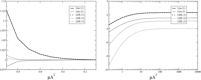
Figure 1: (Left) Ratio of the dispersion relation from Eqs.  (18) and (21)-(23) exactly for $\mu A^{2}<0$ and (right) relative error $\Delta$ [see eq. (24)] of the dispersion relations for $\mu A^{2}\gg 0$.

III Further Examples

III.1 Sine-Gordon model

We now consider the Sine-Gordon model, which is governed by the potential

$$V(u)=-\cos{u}$$ (25)

and which allows us to write the nonlinear Klein-Gordon equation, also known as the Sine-Gordon equation as

$$\Omega^{2}\ddot{u}+\sin{u}=0\;.$$ (26)

The exact dispersion relation in this case can be obtained from

$$\Omega=\frac{\pi}{2\int_{0}^{\pi/2}(1-m^{2}\sin^{2}{t})^{-1/2}dt}$$ (27)

with $m=\sin(A/2)$. Observe that in this case

$$T=4\int_{0}^{\pi/2}(1-m^{2}\sin^{2}{t})^{-1/2}dt\equiv 4K(m^{2})\;,$$ (28)

with $K(m)$ being the elliptic integral of the first kind. We take advantage of this fact and make use of the nonperturbative series for the elliptic integral which was derived using the LDE technique chavos . At order $N$, setting $\lambda=-m/2$ and $\delta=1$, it is given by the expression:

$$K_{N}(m,\lambda)=\frac{\pi}{2}\ \sum_{k=0}^{N}\sum_{j=0}^{k}\frac{\Gamma(j+1/2)}{j!^{2}\,(k-j)!\,\Gamma(1/2-k)}\ \frac{(-m)^{k}}{2^{k-j}\ (1-\frac{m}{2})^{k+1/2}}\;.$$ (29)

This expression provides a nonperturbative series for the elliptic integral of the first kind since it does not correspond to a simple polynomial in $m$.

To further improve this series we can use the Landen transformation AbrSte

$$K(m)=\frac{1}{1+\sqrt{m}}K\left(\frac{4\sqrt{m}}{(1+\sqrt{m})^{2}}\right)$$ (30)

and the inverse relation

$$K(m)=\frac{2(1-\sqrt{1-m})}{m}K\left(\frac{(-2+2\sqrt{1-m}+m)^{2}}{m^{2}}\right)\;.$$ (31)

Notice that $f(m)=\frac{4\sqrt{m}}{(1+\sqrt{m})^{2}}$ maps a value $0<m<1$ into a new value $m^{\prime}=f(m)>m$. The inverse transformation $f^{-1}(m)=\frac{(-2+2\sqrt{1-m}+m)^{2}}{m^{2}}$ maps a value $m$ into a smaller one. Using this transformation we obtain more accurate approximations for the elliptic integrals. For example, at order 1 we find

$$K_{LDE\,(1)}(m)=\frac{\pi}{\sqrt{1-\frac{m}{2}+3\sqrt{1-m}}}$$ (32)

and, correspondingly

$$\Omega_{LDE\,(1)} = \frac{1}{4}\sqrt{\cos(A)+12\left|\cos\left(\frac{A}{2}\right)\right|+3}\;.$$ (33)

At second order we find

$$\Omega_{LDE\,(2)} = \frac{16\cos^{2}{\left(\frac{A}{4}\right)}(3+12\cos{\left(\frac{A}{2}\right)+\cos(A)})^{2}\sqrt{2+2\cos{\left(\frac{A}{2}\right)}\sec^{4}{\left(\frac{A}{4}\right)}}}{2713+2520\cos{\left(\frac{A}{2}\right)+2580\cos{(A)}+360\cos{\left(\frac{3A}{2}\right)+19\cos(2A)}}}\;$$ (34)

It is noticeable that $\Omega_{LDE\,(3)}=\Omega_{LDE\,(2)}$. In fact, for the following consecutive orders, the same statement holds, i. e., $\Omega_{LDE\,(5)}=\Omega_{LDE\,(4)},\,\Omega_{LDE\,(7)}=\Omega_{LDE\,(6)}$ and so on. The same pattern of equal value of the observables for consecutive orders of approximation was found in Ref. AL04 for the Duffing potential at large $n.$

For comparison, Lim et al. Lim have found the dispersion relation to be given at first order as

$$\Omega_{Lim(1)}=\sqrt{\frac{2J_{1}(A)}{A}}\;,$$ (35)

and at second order as

$$\Omega_{Lim(2)}=\sqrt{g(A)+\sqrt{g^{2}(A)-h(A)}}\;,$$ (36)

where

$$g(A) = \frac{(b_{0}-b_{2}-b_{4}+b_{6})A+18a_{1}+2a_{3}}{36A}$$

$$h(A) = \frac{a_{1}(b_{0}-b_{2}-b_{4}+b_{6})}{18A}$$ (37)

and

$$a_{1}=2J_{1}(A),\quad a_{3}=-2J_{3}(A),\quad b_{2i}=2(-1)^{i}J_{2i}(A),\quad i=0,1,2,3$$ (38)

$J_{n}(A)$ being the Bessel function of the first kind.

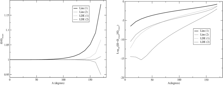
Figure 2: (Left) Ratio of the dispersion relation from eqs.  (33)-(36) exactly and (right) relative error $\Delta$ [see eq. (24)] of the dispersion relations.

In the left-hand panel of Fig. 2 we display the ratio of the dispersion relations from Eqs. (33)-(36) to the exact and on the right-hand panel the corresponding relative errors. From the graphs we see that the LDE curves calculated to second order display much smaller errors than the curves obtained with the method of Lim et al. even close to $A=\pi$. A second observation is that our formulas can be systematically improved simply by going to a higher order and that they do not involve any special function, as in the case of Eq. (35).

III.2 Pure quartic potential

Our final example is the Klein-Gordon equation in a pure quartic potential

$$V(u)=\frac{u^{4}}{4}\;,$$ (39)

which leads to the equation of motion

$$\ddot{u}+u^{3}=0\;.$$ (40)

This is a particular case of the first example where the contribution of the quadratic term in the potential (8) is neglected. As such, the corresponding dispersion relation can be derived from the expression of the period of oscillations, Eq. (19), since the quadratic term contributes with the $4$ in the square root in the front of the double sum and in the argument in the sum, and is simply given by

$$T_{LDE\,(N)}=\frac{4\pi}{\sqrt{3\mu A^{2}}}\sum_{n=0}^{N}(-1)^{n}\left(\begin{array}[]{c}-1/2\\ n\end{array}\right)\left(\begin{array}[]{c}-1/2\\ 2n\end{array}\right)\frac{1}{3^{2n}}\;$$ (41)

and correspondingly $\Omega_{LDE\,(N)}$ can be obtained as in Eq. (20).

Results for the first three orders are the following :

$$\Omega_{LDE\,(1)} = \frac{24\sqrt{3}A}{49}\;,$$ (42)

$$\Omega_{LDE\,(2)} = \frac{13824\sqrt{3}A}{28259}\;,$$ (43)

$$\Omega_{LDE\,(3)} = \frac{1990656\sqrt{3}A}{4069681}\;.$$ (44)

Lim et al. found, at first and second order of approximation, respectively,

$$\Omega_{Lim(1)} = \frac{\sqrt{3}}{2}A\;,$$

$$\Omega_{Lim(2)} = \frac{1}{12}\sqrt{62+2\sqrt{421}}A\;.$$ (45)

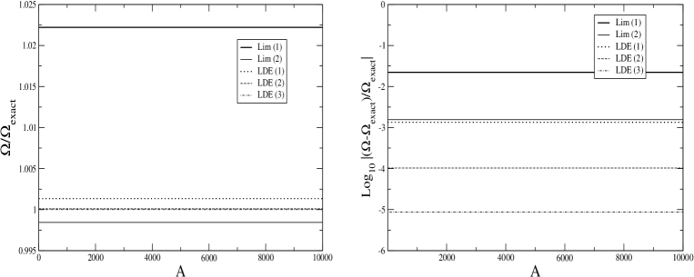
Figure 3: (Left) Ratio of the dispersion relation from Eqs.  (42)-(44), and both expressions in Eq. (45) exactly and (right) relative error $\Delta$ (see eq. (24)) of the dispersion relations.

In the left-hand panel of Fig. 3 we display the ratio of the approximate to the exact dispersion relation and in the right-hand panel the relative error from our findings at first, second and third order and those of Ref. Lim given previously. At first order, our findings perform just as the second order of Lim et al. Lim , and at second and third orders, the performance of the variational results is excellent.

IV Conclusions

We have derived analytical expressions for the dispersion relations of the nonlinear Klein-Gordon equation for different potentials by means of the Linear Delta Expansion. This technique is implemented by computing the period of oscillations in the given potential. In the particular example of the Sine-Gordon potential, where the dispersion relation is given in terms of elliptic integrals, we have implemented the LDE to compute such integral and, by means of the Landen transformation, we have obtained an improved series for the elliptic integral. We have observed that the expression obtained by using the first few terms in this series performs remarkably well even close to the $A=\pi$. We believe that our results are appealing in two respects: first in that they provide a systematic way to approximate the exact result with the desired accuracy, and second in that the expressions that we obtain never involve special functions, as in the case of Ref. Lim . An aspect that needs to be underlined is that the method described in subsection II provides a convergent series representation for the dispersion relation, provided that the arbitrary parameter fulfills a simple condition.

- (1) C. W. Lim, B. S. Wu, and L. H. He. Chaos 4 843, (2001).
- (2) P. Amore and A. Aranda, Phys. Lett. A 316, 218 (2003).
- (3) P. Amore and H. Montes Lamas, Phys. Lett. A 327, 158 (2004).
- (4) P. Amore and A. Aranda, Journal of Sound and Vibration, 283/3-5 pp. 1111-1132 (2005).
- (5) P. Amore and R. A. Sáenz, Europhysics Letters 70 425-431 (2005).
- (6) P. Amore, A. Aranda, R. Sáenz, and F. M. Fernández, Phys. Rev. E 71 , 016704 (2005).
- (7) J. Killingbeck, J. Phys. A 14, 1005 (1980).
- (8) G. A. Arteca, F. M. Fernández, and E. A. Castro, Large order perturbation theory and summation methods in quantum mechanics (Springer, Berlin, Heidelberg, New York, London, Paris, Tokyo, Hong Kong, Barcelona, 1990).
- (9) F. M. Fernández, Introduction to Perturbation Theory in Quantum Mechanics (CRC Press, Boca Raton, 2000).
- (10) A. Okopińska, Phys. Rev. D 35, 1835 (1987); A. Duncan and M. Moshe, Phys. Lett. B 215, 352 (1988).
- (11) P. M. Stevenson, Phys. Rev. D 23, 2916 (1981).
- (12) P. Amore et al., sent to the European Journal of Physics.
- (13) M. Abramowitz and I. A. Stegun, Handbook of Mathematical Functions. Ed. Dover, New York, (1972).