Abstract: For low density gases the validity of the Boltzmann transport equation is well established. The central object is the one-particle distribution function, $f$, which in the Boltzmann-Grad limit satisfies the Boltzmann equation. Grad and, much refined, Cercignani argue for the existence of this limit on the basis of the BBGKY hierarchy for hard spheres. At least for a short kinetic time span, the argument can be made mathematically precise following the seminal work of Lanford. In this article a corresponding program is undertaken for weakly nonlinear, both discrete and continuum, wave equations. Our working example is the harmonic lattice with a weakly nonquadratic on-site potential. We argue that the role of the Boltzmann $f$-function is taken over by the Wigner function, which is a very convenient device to filter the slow degrees of freedom. The Wigner function, so to speak, labels locally the covariances of dynamically almost stationary measures. One route to the phonon Boltzmann equation is a Gaussian decoupling, which is based on the fact that the purely harmonic dynamics has very good mixing properties. As a further approach the expansion in terms of Feynman diagrams is outlined. Both methods are extended to the quantized version of the weakly nonlinear wave equation.

The resulting phonon Boltzmann equation has been hardly studied on a rigorous level. As one novel contribution we establish that the spatially homogeneous stationary solutions are precisely the thermal Wigner functions. For three phonon processes such a result requires extra conditions on the dispersion law. We also outline the reasoning leading to Fourier’s law for heat conduction.

1 Goals and Introduction

Dielectric crystals, as Si and GaAs, have their electronic bands completely filled and separated by an energy gap from the conduction band. Therefore electronic energy transport is suppressed and the dominant contribution to heat transport is due to the vibrations of the atoms around their mechanical equilibrium position. Below room temperature these deviations are small, typically only a few percent of the lattice constant, hence by necessity weakly anharmonic. As envisioned by R. Peierls in 1929 [1], the obvious theoretical option is to regard the anharmonicities as a, in a certain sense, small perturbation to the perfectly harmonic crystal, which at the very end leads to a kinetic description of an interacting “gas of phonons” in terms of a nonlinear Boltzmann transport equation. The actual computation of the thermal conductivity of dielectric crystals is then based on the phonon Boltzmann equation. Through the work of many, for example see [2, 3, 4, 5], it has become apparent that such a program can be made to work resulting in a reliable prediction over a considerable temperature range. Only recently the kinetic description has been augmented by molecular dynamics, which numerically solves the classical equations of motion, see for example [6]. To determine the thermal conductivity one computes either the Green-Kubo formula in an equilibrium system at a fixed temperature or the average energy flux in the steady state with a temperature difference imposed at the boundaries.

In this note I focus on the step from the weakly anharmonic lattice dynamics to the kinetic equation. As an aside, I discuss a few basic properties of the phonon Boltzmann equation, mostly to provide some indication on the physics which persists on the kinetic level but also to advertise an evolution equation which apparently has received little attention.

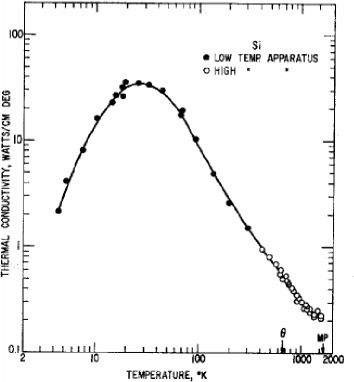
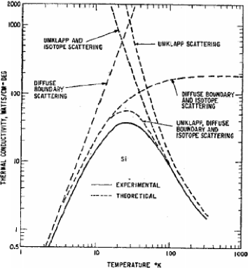
Figure 1: Thermal conductivity of Si (natural abundance)[7].

If the goal is to compute the thermal conductivity of real crystals, the derivation of the Boltzmann equation is considered as a minor issue, where the emphasis varies from author to author. Much more relevant is to have reliable information on the lattice structure, on the phonon dispersion law, and on the lowest order anharmonic elastic constants. Furthermore, on the kinetic level the conductivity is determined through the inverse of the linearized collision operator, which cannot be computed by hand. Hence suitable approximation schemes had to be developed. I will have nothing to say on these topics.

On a qualitative level kinetic theory provides a rather simple picture for the temperature dependence of the thermal conductivity, $\kappa(T)$. At “high” temperatures a semiclassical approximation suffices, which predicts $\kappa(T)=\theta_{\textrm{h}}/T$ with some temperature independent coefficient $\theta_{\textrm{h}}$. At “low” temperatures the quantization of lattice vibrations must be taken into account. The total number of phonons then equals $\int d^{3}k(e^{\omega(k)/k_{\textrm{B}}T}-1)^{-1}$ which reflects the freezing of the number of energy carriers as $T\to 0$. On the other hand also momentum nonconserving collisions become rare, resulting in a phonon mean free path which diverges as $T\to 0$. This latter effect dominates and yields the prediction $\kappa(T)=e^{\theta_{\textrm{l}}/T}$, $\theta_{\textrm{l}}>0$, as $T\to 0$. Experimentally such a behavior is masked by the finite size of the sample and only over a narrow temperature range the exponential increase in $1/T$ can be seen. A crucial point in the experiment is to manufacture a crystal which has no dislocations and is free of impurities. Even then, isotope disorder provides an additional mechanism for diffusive energy transport, which persists in the harmonic approximation. E.g., for Si the natural abundance is ²⁸Si 92.23%, ²⁹Si 4.76%, and ³⁰Si 3.01%, which means that the deviation from the perfect constant atomic mass crystal can be considered as small.

To provide an example we reproduce in Figure 1 the thermal conductivity for chemically pure and dislocation free Si as measured by Glassbrenner and Slack [7]. On the right hand side the importance of the various scattering mechanisms is displayed. Above 100^∘K one notes the classical 1/T-behavior. Below 100^∘K the quantization of phonons becomes relevant. Diffuse boundary scattering reflects the size of the probe which is 2 cm long times 0.44 cm as average diameter. The umklapp scattering refers to momentum nonconserving collisions, see Section 4. The experimental findings are well reproduced by the theory [4], which is based on the linearized Boltzmann equation, as will be explained in Section 14.

In the kinetic theory of gases the central object is the Boltzmann distribution function $Nf(r,v,t)$, $N$ the total number of particles, which counts the number of gas molecules in the volume element $d^{3}rd^{3}v$ in the one-particle phase space close to $r,v$ at time $t$. Phonons are not such local objects. In fact, upon specifying the complete displacement field, including its velocities, it is not so clear how to extract from it the positions and momenta of the particle-like objects called phonons. Most likely, for a general displacement field no such procedure can be devised. Still in the kinetic limit the mechanical picture becomes precise. As has been recognized for some time [8, 9], the link between a wave field and transport equations allowing for a mechanical interpretation is provided by the Wigner function. This approach will be followed also in these notes, noting already now that the collision between phonons, while they conserve energy and momentum, are otherwise unlike collisions between mechanical point particles.

For the purpose of a better understanding of the validity of the kinetic description, my guiding principle is to discard all details and to devise the arguably simplest of all models, which still displays the same physics. I will even go as far as to ignore the obvious fact that atoms deviate in three-space from their equilibrium position. Hence I will assume that the displacement field is scalar. The virtue, I hope, is to make the derivation of the transport equation maximally transparent.

We propose to ignore quantization in the first round. One reason is the hope that for a classical model techniques different from a hierarchy of correlation functions and Feynman diagrams might become available. As a further bonus, we establish the link to weakly anharmonic, in general multicomponent, wave equations, which are applied in the wave dynamics of the upper ocean, in acoustic turbulence, and in other areas [10]. In this context the phenomenon of interest is a turbulent state maintained through external forcing. Again, kinetic theory is the natural theoretical tool to explain and predict properties of the steady state.
Acknowledgements: I am most grateful to Jani Lukkarinen for many instructive discussions and a first reading of the notes. I thank Carlo Cercignani for help towards the H-theorem and Eric Carlen for discussions on the Brout-Prigogine equation. These notes were first presented as lectures at the workshop “Quantum Dynamics and Quantum Transport”, Warwick, September 6 - 12, 2004. I am grateful to Gero Friesecke for this opportunity.

2 A real crystal simplified

We consider the simple cubic lattice $\mathbb{Z}^{3}$ as the lattice of mechanical equilibrium positions of the crystal atoms. The deviations from their equilibrium position are denoted by

$$q_{x}\in\mathbb{R}\,,\quad x\in\mathbb{Z}^{3}\,,$$ (2.1)

with the canonically conjugate momenta

$$p_{x}\in\mathbb{R}\,,\quad x\in\mathbb{Z}^{3}\,.$$ (2.2)

We will use units in which the mass $m$ of an atom equals one. For small deviations from the equilibrium position we may use the harmonic approximation in lowest order. The corresponding potential energy then reads

$$U_{\textrm{harm}}(q)=\frac{1}{2}\sum_{x,y\in\mathbb{Z}^{3}}\alpha(x-y)q_{x}q_{y}\,.$$ (2.3)

The elastic constants $\alpha(x)$ satisfy

$$\alpha(x)=\alpha(-x)\,,\quad|\alpha(x)|\leq\alpha_{0}e^{-\alpha_{1}|x|}$$ (2.4)

for suitable $\alpha_{0},\alpha_{1}>0$, and

$$\sum_{x\in\mathbb{Z}^{3}}\alpha(x)=0$$ (2.5)

because of the invariance of the interaction between the crystal atoms under the translation $q_{x}\rightsquigarrow q_{x}+a$. Mechanical stability requires

$$\widehat{\alpha}(k)>0\quad\textrm{for}\quad k\neq 0$$ (2.6)

for the Fourier transform $\widehat{\alpha}$ of $\alpha$.

The anharmonicity is assumed to reside only in the on-site potential which we divide into a harmonic piece and the rest

$$U_{\textrm{site}}=\sum_{x\in\mathbb{Z}^{3}}\big{(}\frac{1}{2}\omega^{2}_{0}q^{2}_{x}+V_{\textrm{an}}(q_{x})\big{)}\,.$$ (2.7)

Physically, the on-site potential is artificial and it would be more natural to assume that the atoms are coupled through a weakly anharmonic pair potential. As we will argue below, in the kinetic limit only the collision rate turns out to be modified. Thus, for the purpose of deriving the kinetic equation, we might as well stick to the somewhat simpler on-site potential.

The Hamiltonian of the anharmonic lattice system is written as the sum

$$H=H_{0}+V\,.$$ (2.8)

$H_{0}$ is the harmonic piece given through

$$H_{0}=\frac{1}{2}\sum_{x\in\mathbb{Z}^{3}}\Big{(}p_{x}^{2}+\omega_{0}^{2}q_{x}^{2}\Big{)}+\frac{1}{2}\sum_{x,y\in\mathbb{Z}^{3}}\alpha(x-y)q_{x}q_{y}\,,$$ (2.9)

$\omega_{0}>0$. The lowest order type of anharmonicity reads

$$V=\sum_{x\in\mathbb{Z}^{3}}V_{\textrm{an}}(q_{x})\,\quad V_{\textrm{an}}(q_{x})=\lambda\frac{1}{3}q^{3}_{x}$$ (2.10)

with $\lambda$ small. The potential energy $U_{\textrm{harm}}+U_{\textrm{site}}$ is then not bounded from below, which however will not be visible on the kinetic time scale. If preferred, one could add to $V_{\textrm{an}}$ the quartic term $\lambda^{\prime}q_{x}^{4}$ with $\lambda^{\prime}=\lambda^{2}/18\omega_{0}^{2}$. Then $H\geq 0$ and the quartic term disappears in the kinetic scaling. For reasons of readability we will set $\lambda^{\prime}=0$.

We work in the physical space dimension. Whether the kinetic approximation is valid in one and two dimensions remains debated. On the other hand only for such low dimensional systems extensive numerical results are available, to which we will turn in Section 17.

The equations of motion are

$$\frac{d}{dt}q_{x}(t)=p_{x}(t)\,,$$

$$\frac{d}{dt}p_{x}(t)=-\sum_{y\in\mathbb{Z}^{3}}\alpha(y-x)q_{y}(t)-\omega_{0}^{2}q_{x}(t)-\lambda q_{x}(t)^{2}\,,\quad x\in\mathbb{Z}^{3}\,.$$ (2.11)

We will consider only finite energy solutions. In particular, it is assumed that $|p_{x}|\to 0$, $|q_{x}|\to 0$ sufficiently fast as $|x|\to\infty$. In fact, later on there will be the need to impose random initial data, which again are assumed to be supported on finite energy configurations. As to be explained in great detail, in the kinetic limit the average energy diverges suitable linked to the nonlinearity $\lambda\to 0$.

We will mostly work in Fourier space and set up the notation. Let $\mathbb{T}^{3}=[-\frac{1}{2},\frac{1}{2}]^{3}$ be the first Brillouin zone of the dual lattice. For $f:\mathbb{Z}^{3}\to\mathbb{R}$ we use the following convention for the Fourier transform,

$$\widehat{f}(k)=\sum_{x\in\mathbb{Z}^{3}}e^{-i2\pi k\cdot x}f_{x}\,,\quad k\in\mathbb{T}^{3}\,.$$ (2.12)

$\widehat{f}(k)$ extends to a $2\pi$-periodic function on $\mathbb{R}^{3}$. The inverse Fourier transform is given by

$$f_{x}=\int_{\mathbb{T}^{3}}dke^{i2\pi k\cdot x}\widehat{f}(k)\,,$$ (2.13)

where $dk$ is the 3-dimensional Lebesgue measure. This convention has the advantage of maximally avoiding prefactors of $2\pi$. The dispersion relation for the harmonic part $H_{0}$ is easily computed as

$$\omega(k)=\big{(}\omega^{2}_{0}+\widehat{\alpha}(k)\big{)}^{1/2}\,.$$ (2.14)

By mechanical stability $\omega(k)\geq\omega_{0}$. If $\omega_{0}>0$, then $\omega$ is a real analytic function on $\mathbb{T}^{3}$. If $\omega_{0}=0$, $\omega$ may still be real analytic, one example being $\widehat{\alpha}(k)\simeq|k|^{4}$ for small $k$. In Fourier space the equations of motion become

$$\frac{\partial}{\partial t}\widehat{q}(k,t)=\widehat{p}(k,t)\,,$$

$$\frac{\partial}{\partial t}\widehat{p}(k,t)=-\omega(k)^{2}\widehat{q}(k,t)$$

$$\hskip 36.0pt-\lambda\int_{\mathbb{T}^{6}}dk_{1}dk_{2}\delta(k-k_{1}-k_{2})\widehat{q}(k_{1},t)\widehat{q}(k_{2},t)$$ (2.15)

with $k\in\mathbb{T}^{3}$. Here $\delta$ is the $\delta$-function on the unit torus, to say, $\delta(k^{\prime})$ carries a point mass whenever $k^{\prime}\in\mathbb{Z}^{3}$.

It will be convenient to concatenate $q_{x}$ and $p_{x}$ into a single complex-valued field. We set

$$a(k)=\frac{1}{\sqrt{2}}\big{(}\sqrt{\omega(k)}\,\widehat{q}(k)+i\frac{1}{\sqrt{\omega(k)}}\,\widehat{p}(k)\big{)}$$ (2.16)

with the inverse

$$\widehat{q}(k)=\frac{1}{\sqrt{2}}\frac{1}{\sqrt{\omega(k)}}\big{(}a(k)+a(-k)^{\ast}\big{)}\,,\;\widehat{p}(k)=\frac{1}{\sqrt{2}}i{\sqrt{\omega(k)}}\big{(}-a(k)+a(-k)^{\ast}\big{)}\,.$$ (2.17)

The $a$-field evolves as

$$\frac{\partial}{\partial t}a(k,t)=-i\omega(k)a(k,t)-i\lambda\int_{\mathbb{T}^{6}}dk_{1}dk_{2}\delta(k-k_{1}-k_{2})$$

$$(8\omega(k)\omega(k_{1})\omega(k_{2}))^{-1/2}(a(k_{1},t)+a(-k_{1},t)^{\ast})(a(k_{2},t)+a(-k_{2},t)^{\ast})\,.$$ (2.18)

In particular for $\lambda=0$,

$$a(k,t)=e^{-i\omega(k)t}a(k)\,.$$ (2.19)

For real crystals the $a$-field would be vector-valued for two reasons: the displacements are in $\mathbb{R}^{3}$ and the unit cell contains usually more than one atom. Correspondingly $\omega$ then becomes a $k$-dependent matrix. Furthermore by translation invariance the potential energy of the crystal depends only on the differences $q_{y}-q_{x}$. As long as the interest is merely in the derivation of the Boltzmann equation such extra features can be ignored.

If one simplifies anyhow, the reader may wonder why we do not switch to the continuum wave equation. In our context a natural option would be the Klein-Gordon equation with a weak quadratic nonlinearity,

$$\frac{\partial^{2}}{\partial t^{2}}\phi(x,t)=\Delta\phi(x,t)-\omega^{2}_{0}\phi(x,t)-\lambda\phi(x,t)^{2}\,,\quad x\in\mathbb{R}^{3}\,.$$ (2.20)

Another possibility would be the standard wave equation with a cubic nonlinearity

$$\frac{\partial^{2}}{\partial t^{2}}\phi(x,t)=\Delta\phi(x,t)-\lambda\phi(x,t)^{3}\,,\quad x\in\mathbb{R}^{3}\,.$$ (2.21)

We will discuss continuum equations in Section 8, from which it will become clear that the underlying lattice structure plays a crucial role.

Having agreed upon the basic model (2) of our enterprise, we have reached a point of bifurcation. Physically we should quantize (2.8), together with (2.9), (2.10), according to the standard rules and then investigate the effects small anharmonicities. On the other hand it seems to be worthwhile not to hurry so much and to explore the classical model, which has an interesting structure of its own. In addition there could be help from the theory of nonlinear wave equations, which would put our claims on firmer ground. Thus in Sections 3 to 6 we treat the derivation of the Boltzmann equation for the classical model. The same program is repeated for the quantized crystal in Sections 9 and 10 with the approach through Feynman diagrams explained in Section 11. In Section 8 we address wave turbulence which is concerned with continuum wave equations such as (2.20) and (2.21). Sections 7 and 12 study properties of Boltzmann equation, in particular the H-theorem. The nonlinear part concludes with a discussion of the thermal conductivity. In the final part of our notes we investigate the harmonic crystal with random isotope substitution.

3 Local stationarity, Wigner function

The kinetic theory of dilute gases relies on the scale separation between typical interatomic distances and the mean free path. As a consequence locally, in regions of linear size much larger than atomic distances and much smaller than the mean free path, the statistics of particles is Poisson in a good approximation. If $f(r,v,t)$ denotes the Boltzmann distribution function at time $t$, then close to $r$ the particles are uniformly distributed with density $\rho(r)=\int d^{3}vf(r,v,t)$ and their velocities are independent with common distribution $f(r,v,t)/\rho(r)$. The Poisson distribution is singled out from all other conceivable distributions, because it is stationary in time with respect to the free gas dynamics, translation invariant in space, and has a strictly positive entropy per unit volume. In fact, there are no other such probability measures [12].

To transcribe this kinetic picture to weakly interacting phonons, as building blocks we need, on the phase space of microscopic configurations $\{q_{x},p_{x},\;x\in\mathbb{Z}^{3}\}$, probability measures which are invariant under the free dynamics generated by $H_{0}$, stationary under lattice shifts, and have a strictly positive entropy per unit volume. The obvious candidates are Gaussian measures with zero mean. By translation invariance, their covariance reads

$$\langle q_{x}q_{y}\rangle=Q(x-y)\,,\quad\langle p_{x}p_{y}\rangle=P(x-y)\,,\quad\langle q_{x}p_{y}\rangle=C(x-y)\,.$$ (3.1)

Let $\widehat{Q}$, $\widehat{P}$, $\widehat{C}$ denote the corresponding Fourier transforms. Then $\widehat{Q}(k)\geq 0$, $\widehat{Q}(k)=\widehat{Q}(-k)$, $\widehat{P}(k)\geq 0$, $\widehat{P}(k)=\widehat{P}(-k)$, $\widehat{C}(k)=\widehat{C}(-k)^{\ast}$, and $|\widehat{C}|^{2}\leq\widehat{Q}\widehat{P}$. Stationarity in time yields in addition the relations

$$\widehat{P}=\omega^{2}\widehat{Q}\,,\quad C(x)=-C(-x)\,,\quad\textrm{i.e.}\;\widehat{C}(k)=-\widehat{C}(-k)\,.$$ (3.2)

Such properties are more concisely expressed through the $a$-field. Stationarity in space-time is equivalent to

$$\langle a(k)\rangle=0\,,\quad\langle a(k)a(k^{\prime})\rangle=0\,,\quad\langle a(k)^{\ast}a(k^{\prime})\rangle=W(k)\delta(k-k^{\prime})\,.$$ (3.3)

$W(k)\geq 0$ and, by convention, $W(k)$ is a $2\pi$-periodic function on $\mathbb{R}^{3}$. Inserting the definition (2.16) and comparing with (3.2) results in

$$\frac{1}{2}\big{(}W(k)+W(-k)\big{)}=\frac{1}{2}\big{(}\omega\widehat{Q}(k)+\frac{1}{\omega}\widehat{P}(k)\big{)}=\omega\widehat{Q}(k)=\frac{1}{\omega}\widehat{P}(k)\,,$$

$$\frac{1}{2}\big{(}W(k)-W(-k)\big{)}=i\widehat{C}(k)\,.$$ (3.4)

The meaning of the covariance $W$ is grasped better by considering expectations of some physical quantities. Let us first study the local energy $H_{x}$, for which we equally divide the potential energy between the two elastically coupled sites. Then

$$H_{x}=\frac{1}{2}p_{x}^{2}+\frac{1}{2}\omega^{2}_{0}q^{2}_{x}+\frac{1}{2}\sum_{y\in\mathbb{Z}^{3}}\alpha(x-y)q_{x}q_{y}$$ (3.5)

and

$$H_{0}=\sum_{x\in\mathbb{Z}^{3}}H_{x}\,.$$ (3.6)

Clearly

$$\langle H_{x}\rangle=\int_{\mathbb{T}^{3}}dk\omega(k)W(k)\,.$$ (3.7)

To probe further, we study the flow of energy out of a big box $\Lambda\subset\mathbb{Z}^{3}$. Setting $H_{\Lambda}=\sum_{x\in\Lambda}H_{x}$ one finds

$$\frac{d}{dt}H_{\Lambda}=\frac{1}{2}\sum_{x\in\Lambda}\sum_{y\in\mathbb{Z}^{3}\setminus\Lambda}\alpha(x-y)(-q_{x}p_{y}+q_{y}p_{x})\,.$$ (3.8)

Since the coupling is not only nearest neighbor, the division into local currents is somewhat arbitrary. To be specific, let us choose as one face of $\Lambda$ the coordinate plane $\{x,x^{1}=0\}$. Then, in the limit $\Lambda\to\infty$, the one-component of the energy current becomes

$$j^{1}_{\mathrm{e}}=\frac{1}{2}\sum_{x^{1}\leq 0}\sum_{y^{1}\geq 1}\alpha(x-y)(-q_{(x^{1},0,0)}p_{y}+q_{y}p_{(x^{1},0,0)})\,.$$ (3.9)

Upon averaging, using (3) and (3.9),

$$\langle j_{\mathrm{e}}\rangle=\frac{1}{4\pi}\int_{\mathbb{T}^{3}}dk\nabla\widehat{\alpha}(k)W(k)=\frac{1}{2\pi}\int_{\mathbb{T}^{3}}dk(\omega\nabla\omega)(k)W(k)\,.$$ (3.10)

Thus it is natural to regard $W$ as number density in wave number space. $\omega W$ is the energy density and $(2\pi)^{-1}\nabla\omega(\omega W)$ is the energy current density. Note that if $W$ is even, the total energy current vanishes.

A further important quantity is the entropy per unit volume, which on general grounds is defined as the logarithm of the phase space volume at prescribed values of the “macrovariables”, see Appendix 18.2 for further discussion. Here we use an equivalent short-cut and compute the Gibbs entropy of the Gaussian measure with covariance given through $W$. To do so let us choose the periodic box $[1,\ell]^{3}$, $\ell$ integer, and consider the finite volume analogue of the Gaussian measure from (3.3). Then $k$ takes the discrete values $k\in(\ell^{-1}[1,...,\ell])^{3}$. Let $\rho_{\textrm{G}}$ be the corresponding probability density. As usual, the entropy of $\rho_{\textrm{G}}$ is given through

$$S_{\ell}=-\int_{\mathbb{R}^{\ell^{3}}}d^{\ell^{3}}qd^{\ell^{3}}p\rho_{\textrm{G}}\log\rho_{\textrm{G}}=\sum_{k\in(\ell^{-1}[1,...,\ell])^{3}}\big{(}\log W(k)+\log\pi+1\big{)}$$ (3.11)

and thus the entropy per unit volume by

$$\lim_{\ell\to\infty}\ell^{-3}S_{\ell}=\int_{\mathbb{T}^{3}}dk\big{(}\log W(k)+\log\pi+1\big{)}\,.$$ (3.12)

The next step is to construct, out of the Gaussian measures introduced in (3.3), Gaussian measures which have a slow variation in physical space $\mathbb{Z}^{3}$ and which are locally stationary. For this purpose we give ourselves the local power spectrum $W(r,k)\geq 0$, $r\in\mathbb{R}^{3}$, which vanishes rapidly as $|r|\to\infty$, and introduce

$$Q(r,x)=\int_{\mathbb{T}^{3}}dkW(r,k)\omega(k)^{-1}\cos(2\pi k\cdot x)\,,$$ (3.13)

$$P(r,x)=\int_{\mathbb{T}^{3}}dkW(r,k)\omega(k)\cos(2\pi k\cdot x)\,,$$

$$C(r,x)=\int_{\mathbb{T}^{3}}dkW(r,k)\sin(2\pi k\cdot x)\,,$$

$x\in\mathbb{Z}^{3}$, by which we define the family $\langle\cdot\rangle^{\textrm{G},\varepsilon}$ of Gaussian measures through

$$\langle q_{x}\rangle^{\textrm{G},\varepsilon}=0\,,\quad\langle p_{x}\rangle^{\textrm{G},\varepsilon}=0\,,$$

$$\langle q_{x}q_{x^{\prime}}\rangle^{\textrm{G},\varepsilon}=Q(\varepsilon(x+x^{\prime})/2,x-x^{\prime})+\mathcal{O}(\varepsilon)\,,$$

$$\langle p_{x}p_{x^{\prime}}\rangle^{\textrm{G},\varepsilon}=P(\varepsilon(x+x^{\prime})/2,x-x^{\prime})+\mathcal{O}(\varepsilon)\,,$$

$$\langle q_{x}p_{x^{\prime}}\rangle^{\textrm{G},\varepsilon}=C(\varepsilon(x+x^{\prime})/2,x-x^{\prime})+\mathcal{O}(\varepsilon)\,.$$ (3.14)

The error of order $\varepsilon$ has to be allowed so to ensure a positive definite covariance matrix.

This family has two important properties.
(i) Relative to the reference point $r/\varepsilon$, $r\in\mathbb{R}^{3}$, the measure becomes stationary in the limit $\varepsilon\to 0$. This is the property of local stationarity.
(ii) For two distinct reference points $r$ and $r^{\prime}$, $r\neq r^{\prime}$, the local distributions become independent in the limit $\varepsilon\to 0$ as can be inferred from

$$\lim_{\varepsilon\to 0}\big{\{}\langle q_{\lfloor r/\varepsilon\rfloor+x}q_{\lfloor r/\varepsilon\rfloor+x^{\prime}}q_{\lfloor r^{\prime}/\varepsilon\rfloor+y}q_{\lfloor r^{\prime}/\varepsilon\rfloor+y^{\prime}}\rangle^{\textrm{G},{\varepsilon}}$$

$$\hskip 10.0pt-\langle q_{\lfloor r/\varepsilon\rfloor+x}q_{\lfloor r/\varepsilon\rfloor+x^{\prime}}\rangle^{\textrm{G},{\varepsilon}}\langle q_{\lfloor r^{\prime}/\varepsilon\rfloor+y}q_{\lfloor r^{\prime}/\varepsilon\rfloor+y^{\prime}}\rangle^{\textrm{G},{\varepsilon}}\big{\}}=0\,,$$ (3.15)

with $\lfloor\cdot\rfloor$ denoting integer part, since $Q(r,x)\to 0$ as $|x|\to\infty$ . The analogous property holds for the remaining covariances. Thus under the Gaussian measure $\langle\cdot\rangle^{\textrm{G},\varepsilon}$ two macroscopically far apart regions are statistically independent.

The construction (3) is computationally not so flexible and it is more convenient to invert the order. Thus the primary object is a family $\langle\cdot\rangle^{\textrm{G},\varepsilon}$ of Gaussian measures (non-Gaussian measures to be discussed further on). They have mean zero and a local covariance, which is almost time stationary and slowly varying in space. These conditions are most easily imposed through the lattice analogue of the local power spectrum $W$ expressed in terms of $a$-field, compare with (3.3). Firstly we require

$$\langle a(k)\rangle^{\textrm{G},\varepsilon}=0\,,\quad\langle a(k)a(k^{\prime})\rangle^{\textrm{G},\varepsilon}=0\,.$$ (3.16)

The local $a^{\ast}a$ spectrum is defined through

$$W^{1}(x,k)=2^{-3}\int_{(2\mathbb{T})^{3}}d\eta e^{i2\pi x\cdot\eta}\langle a(k-\eta/2)^{\ast}a(k+\eta/2)\rangle^{\textrm{G},\varepsilon}\,.$$ (3.17)

$\langle a(k-\eta/2)^{\ast}a(k+\eta/2)\rangle^{\textrm{G},\varepsilon}$ is $\mathbb{T}^{3}$-periodic in $k$ and $(2\mathbb{T})^{3}$-periodic in $\eta$. Therefore $W(x,k)$ as inverse Fourier transform with respect to $\eta$ is $\mathbb{T}^{3}$-periodic in $k$ and lives on the half-integer lattice $(\mathbb{Z}/2)^{3}$ with respect to $x$.

We rescale the lattice to have lattice spacing $\varepsilon$ through the substitution $x=\varepsilon^{-1}y$, $y\in(\varepsilon\mathbb{Z}/2)^{3}$, and obtain the rescaled local power spectrum

$$W^{\varepsilon}(y,k)=(\varepsilon/2)^{3}\int_{(2\mathbb{T}/\varepsilon)^{3}}d\eta e^{i2\pi y\cdot\eta}\langle a(k-\varepsilon\eta/2)^{\ast}a(k+\varepsilon\eta/2)\rangle^{\textrm{G},\varepsilon}\,.$$ (3.18)

Then, denoting $\lfloor\cdot\rfloor_{\varepsilon}$ as modulo $\varepsilon$, one requires

$$\lim_{\varepsilon\to 0}W^{\varepsilon}(\lfloor r\rfloor_{\varepsilon},k)=W(r,k)$$ (3.19)

pointwise. If $\langle\cdot\rangle^{\textrm{G},\varepsilon}$ is defined through (3), then $W$ of (3.19) agrees with the one in (3.13). $W^{\varepsilon}(y,k)$ is normalized as

$$\sum_{y\in(\varepsilon\mathbb{Z}/2)^{3}}\int_{\mathbb{T}^{3}}dkW^{\varepsilon}(y,k)=\int_{\mathbb{T}^{3}}dk\langle a(k)^{\ast}a(k)\rangle^{\textrm{G},\varepsilon}\,.$$ (3.20)

The condition that the limit in (3.19) exists thus implies that the average phonon number increases as $\varepsilon^{-3}$, equivalently the average total energy increases as

$$\int_{\mathbb{T}^{3}}dk\omega(k)\langle a(k)^{\ast}a(k)\rangle^{\textrm{G},\varepsilon}=\langle H_{0}\rangle^{\textrm{G},\epsilon}=\mathcal{O}(\varepsilon^{-3})\,.$$ (3.21)

(3.18) has a familiar touch. Recall that for a quantum wave function $\psi$ on physical space $\mathbb{R}^{3}$ the Wigner function is defined by

$$W^{\varepsilon}(x,k)=\int_{\mathbb{R}^{3}}d\eta e^{ix\cdot\eta}\widehat{\psi}(k-\varepsilon\eta/2)^{\ast}\widehat{\psi}(k+\varepsilon\eta/2)$$ (3.22)

with $x,k\in\mathbb{R}^{3}$ and $\widehat{\psi}$ the Fourier transform of $\psi$. $\varepsilon$ is the semiclassical parameter, $\varepsilon\to 0$ in the semiclassical limit. The main difference to (3.18) is that for the semiclassical limit usually one considers a sequence $\psi^{\varepsilon}$ of wave functions, while in (3.18) one has a sequence of probability measures over the wave field and its time derivative. Because of this obvious analogy we call (3.18) the Wigner function, more properly the one-point Wigner function. The $n$-point Wigner function is understood as the $n$-th moment of $a^{\ast}a$.

For a family $\langle\cdot\rangle^{\varepsilon}$ of general measures on phase space one defines the one-point Wigner function

$$W^{\varepsilon}(y,k)=(\varepsilon/2)^{3}\int_{(2\mathbb{T}/\varepsilon)^{3}}d\eta e^{i2\pi y\cdot\eta}\langle a(k-\varepsilon\eta/2)^{\ast}a(k+\varepsilon\eta/2)\rangle^{\varepsilon}\,,$$ (3.23)

i.e. through (3.18) with $\langle\cdot\rangle^{\textrm{G},\varepsilon}$ replaced by $\langle\cdot\rangle^{\varepsilon}$. The rescaled two-point Wigner function becomes

$$W^{\varepsilon}(y_{1},k_{1},y_{2},k_{2})=(\varepsilon/2)^{6}\int_{(2\mathbb{T}/\varepsilon)^{6}}d\eta_{1}d\eta_{2}\exp[i2\pi y_{1}\cdot\eta_{1}+i2\pi y_{2}\cdot\eta_{2}]$$

$$\langle a(k_{1}-\varepsilon\eta_{1}/2)^{\ast}a(k_{1}+\varepsilon\eta_{1}/2)a(k_{2}-\varepsilon\eta_{2}/2)^{\ast}a(k_{2}+\varepsilon\eta_{2}/2)\rangle^{\varepsilon}\,,$$ (3.24)

and similarly for higher-point Wigner functions. We require (3.19) and

$$\lim_{\varepsilon\to 0}\langle\prod^{m}_{j=1}a(k_{j})^{\ast}\prod^{n}_{i=1}a(k_{i}^{\prime})\rangle^{\varepsilon}=0$$ (3.25)

whenever $m\neq n$. The condition of statistical independence of far apart regions then reads

$$\lim_{\varepsilon\to 0}\{W^{\varepsilon}(\lfloor r_{1}\rfloor_{\varepsilon},k_{1},\lfloor r_{2}\rfloor_{\varepsilon},k_{2})-W^{\varepsilon}(\lfloor r_{1}\rfloor_{\varepsilon},k_{1})W^{\varepsilon}(\lfloor r_{2}\rfloor_{\varepsilon},k_{2})\}=0$$ (3.26)

for $r_{1}\neq r_{2}$, which in the context of low density gases is known as assumption of molecular chaos. Since (3.26) is a law of large numbers, it implies that

$$\lim_{\varepsilon\to 0}W^{\varepsilon}(\lfloor r_{1}\rfloor_{\varepsilon},k_{1},\ldots,\lfloor r_{n}\rfloor_{\varepsilon},k_{n})=\prod^{n}_{j=1}W(\lfloor r_{j}\rfloor_{\varepsilon},k_{j})$$ (3.27)

whenever the family $\{r_{1},\ldots,r_{n}\}$ is free of double points.

There is no reason that $\langle\cdot\rangle^{\varepsilon}$ becomes locally stationary as $\varepsilon\to 0$. Still the condition of local stationarity can be expressed through the limiting behavior of multi-point Wigner functions. For example, in the case of the two-point function the condition would read

$$\lim_{\varepsilon\to 0}W^{\varepsilon}(\lfloor r\rfloor_{\varepsilon},k_{1},\lfloor r\rfloor_{\varepsilon},k_{2})=W(r,k_{1})W(r,k_{2})$$ (3.28)

$$+\delta(k_{1}+k_{2})\int_{\mathbb{T}^{3}}d\eta W(r,k_{1}+\eta/2)W(r,k_{2}+\eta/2)\,.$$

For a sequence $\langle\cdot\rangle^{\textrm{G},\varepsilon}$ of Gaussian measures satisfying (3.19) the identity (3.28) holds by construction.

4 Kinetic limit

As initial measures for (2) we adopt the scale of Gaussian measures $\langle\cdot\rangle^{\textrm{G},\varepsilon}$ satisfying (3.16) - (3.19). The time-evolved measure at time $t$ is denoted by $\langle\cdot\rangle_{t}$. Let us first consider the harmonic lattice dynamics, $\lambda=0$. Then by linearity, $\langle\cdot\rangle_{t}$ is again Gaussian. Since the deviations from stationarity are on the spatial scale $\varepsilon^{-1}$ and since there is a finite speed of propagation, one has to wait for times of order $\varepsilon^{-1}t$ to observe appreciable changes of the Wigner function, which defines the kinetic time scale $\varepsilon^{-1}t$. On that scale one has

$$\frac{\partial}{\partial t}\langle a(k-\varepsilon\eta/2)^{\ast}a(k+\varepsilon\eta/2)\rangle_{t/\varepsilon,}$$

$$=-i\varepsilon^{-1}\big{(}\omega(k+\varepsilon\eta/2)-\omega(k-\varepsilon\eta/2)\big{)}\;\langle a(k-\varepsilon\eta/2)^{\ast}a(k+\varepsilon\eta/2)\rangle_{t/\varepsilon}\,.$$ (4.1)

Taking the limit $\varepsilon\to 0$ one obtains

$$\frac{\partial}{\partial t}\widehat{W}(\eta,k,t)=-i\nabla\omega(k)\cdot\eta\widehat{W}(\eta,k,t)$$ (4.2)

and, upon inverting the Fourier transform, the limit Wigner function is the solution of the transport equation

$$\frac{\partial}{\partial t}W(r,k,t)=-\frac{1}{2\pi}\nabla\omega(k)\cdot\nabla_{r}W(r,k,t)\,.$$ (4.3)

Thus in the kinetic limit, $\varepsilon\to 0$, we can think of the phonon counting function $W$ as arising from a gas of independent particles, the phonons, with kinetic energy $\omega(k)$. Detailed proofs for the validity of the free transport equation (4.3) are given by Mielke [13]. He allows for rather general deterministic initial data and for harmonic lattice dynamics with vector displacements and a general unit cell.

If one adjusts the strength of collisions in such a way as to have an effect of the same order as the transport term, then kinetic theory claims that the locally stationary state imposed at $t=0$ retains its structure in the course of time. Of course, the time-evolved measure $\langle\cdot\rangle_{t/\varepsilon}$ is no longer exactly Gaussian. But for small $\varepsilon$ and on a local scale it does remain so in a good approximation. As crucial difference to (4.3) the evolution equation will contain a collision term taking account of the anharmonicities. As to be shown in the following section, the cubic term is of the right strength if one substitutes

$$\lambda\rightsquigarrow\sqrt{\varepsilon}\lambda$$ (4.4)

with $\lambda$ fixed and independent of $\varepsilon$. Then the stabilizing quartic term has the strength $\lambda^{\prime}=(\lambda^{2}/18\omega_{0}^{2})\varepsilon$, which is indeed small compared to the cubic term. The Wigner function at the kinetic time $t$ is given through

$$W^{\varepsilon}(y,k,t)=\varepsilon^{3}\int_{(\mathbb{T}/\varepsilon)^{3}}d\eta e^{i2\pi y\cdot\eta}\langle a(k-\varepsilon\eta/2)^{\ast}a(k+\varepsilon\eta/2)\rangle_{t/\varepsilon}\,.$$ (4.5)

It is expected that the limit $\varepsilon\to 0$ exists,

$$\lim_{\varepsilon\to 0}W^{\varepsilon}(\lfloor r\rfloor_{\varepsilon},k,t)=W(r,k,t)\,,$$ (4.6)

and the limit phonon counting function $W$ is the solution of a Boltzmann-like equation. Its derivation will be explained in the section to follow, but let us state the result already now,

$$\frac{\partial}{\partial t}W(r,k,t)+\frac{1}{2\pi}\nabla\omega(k)\cdot\nabla_{r}W(r,k,t)$$ (4.7)

$$=\gamma\int_{\mathbb{T}^{6}}dk_{1}dk_{2}(\omega(k)\omega(k_{1})\omega(k_{2}))^{-1}\big{\{}2\delta(\omega(k)+\omega(k_{1})-\omega(k_{2}))\delta(k+k_{1}-k_{2})$$

$$\hskip 16.0pt\big{(}W(r,k_{1},t)W(r,k_{2},t)+W(r,k,t)W(r,k_{2},t)-W(r,k,t)W(r,k_{1},t)\big{)}\hskip 20.0pt\textrm{(I)}$$

$$\hskip 16.0pt+\;\delta(\omega(k)-\omega(k_{1})-\omega(k_{2}))\delta(k-k_{1}-k_{2})$$

$$\hskip 16.0pt\big{(}W(r,k_{1},t)W(r,k_{2},t)-W(r,k,t)W(r,k_{1},t)-W(r,k,t)W(r,k_{2},t)\big{)}\big{\}}\quad\textrm{(II)}$$

with $\gamma$ the strength of the collision term,

$$\gamma=\frac{\pi}{2}\lambda^{2}\,.$$ (4.8)

$\delta$ is the torus $\delta$-function, see the explanation below Equation (2). As shorthand the collision operator is denoted by $\mathcal{C}(W)$.

Figure 2: Three phonon collisions.

Dynamically the terms (I) and (II) can be viewed as given in Figure 2. In (I) the phonon with wave vector $k$ collides with a phonon with wave vector $k_{1}$ in order to merge into a phonon with wave vector $k_{2}$. The loss term is the term proportional to $W(k)$, hence $2W(k)(W(k_{2})-W(k_{1}))$, and the gain term is the remainder, i.e. $2W(k_{1})W(k_{2})$. Note that the gain term has a definite sign while the loss term takes both signs. Correspondingly in (II) the phonon with wave vector $k$ splits into two phonons with wave vector $k_{1}$ and $k_{2}$. The gain term is again $W(k_{1})W(k_{2})$ and the loss term is $-W(k)(W(k_{1})+W(k_{2}))$. The precise way of how the phonon distribution functions appear in (4.7) does not seem to have a mechanical interpretation in terms of colliding point particles. As can be seen from the $\delta$-functions in the collision operator, in both collision processes energy is conserved, while momentum is conserved only modulo integers. E.g. for term (I) the $\delta$-function yields the constraint

$$k+k_{1}=k_{2}+n\,,\quad n\in\mathbb{Z}^{3}\,,\quad k,k_{1},k_{2}\in\mathbb{T}^{3}\,.$$ (4.9)

In case $n=0$ one speaks of a normal process while in case $n\neq 0$ of an umklapp process.

The rates appearing in (I) and (II) come out of the computation to be presented in Section 6. However, their relative strength $1/2$ is required in order for energy to be locally conserved.

Note that the Boltzmann equation preserves the positivity of $W$. Obviously the free streaming term has this property. If $W$ first hits 0 at some point $k$, $W(r,k,t)=0$, then $dW(r,k,t)/dt>0$, $d/dt$ denoting the total time derivative, due to the positive gain term and vanishing loss term of the collision operator. Hence at that point $W$ cannot turn negative.

This seems to be a good moment to return to the issue of a potential energy which depends only on the differences in the displacements, as would be the case for a real crystal. Then $\omega_{0}=0$ and $V$ of (2.10) is replaced by

$$V_{3}=\lambda\frac{1}{3}\sum_{x\in\mathbb{Z}^{3}}\sum_{\alpha=1}^{3}(q_{x+e_{\alpha}}-q_{x})^{3}\,,$$ (4.10)

$e_{1},e_{2},e_{3}$ the standard basis of $\mathbb{Z}^{3}$, which expressed in terms of the $a$-fields becomes

$$V_{3}=\lambda\frac{1}{3}\sum_{\alpha=1}^{3}\int_{\mathbb{T}^{9}}dk_{1}dk_{2}dk_{3}\delta(k_{1}+k_{2}+k_{3})$$

$$\hskip 30.0pt\prod^{3}_{j=1}\big{\{}(2\omega(k_{j}))^{-1/2}(\exp[i2\pi k^{\alpha}_{j}]-1)(a(k_{j})+a(-k_{j})^{\ast})\big{\}}\,.$$ (4.11)

Compared to $V$ of (2.10), only the weight in Fourier space has changed. Thus the Boltzmann equation remains as in (4.7) provided the collision rate $(\omega(k)\omega(k_{1})\omega(k_{2}))^{-1}$ is replaced by

$$\prod^{3}_{j=1}\big{|}\sum_{\alpha=1}^{3}\omega(k_{j})^{-1/2}(\exp[i2\pi k^{\alpha}_{j}]-1)\big{|}^{2}\,,\quad k_{3}=k\,.$$ (4.12)

Close to the origin this collision rate is more singular than the one in (4.7). But the general properties of the Boltzmann equation, as to be discussed in Section 7, remain in force.

We hurried a little bit to write down the Boltzmann equation. So the reader might wonder why we claim that on the kinetic time scale local stationarity is maintained. The point is that the free dynamics, generated by $H_{0}$, does not tolerate deviations from local stationarity as long as the free dynamics is given some time act. Such a property has been studied in considerable detail by Dobrushin et al. [14], for recent improvements see [15]. Roughly speaking, they consider initial measures $\langle\cdot\rangle^{\varepsilon}$ on phase space for which $\langle q_{x}\rangle^{\varepsilon}=0=\langle p_{x}\rangle^{\varepsilon}$ and for which the Wigner function $W^{\varepsilon}$ of (3.23) has a limit as in (3.19). In addition they require that under $\langle\cdot\rangle^{\varepsilon}$ spatial regions separated by a distance $\ell$ with $1\ll\ell\ll\varepsilon^{-1}$ are in essence statistically independent. $\langle\cdot\rangle^{\varepsilon}$ is non-Gaussian, in general. This initial state is evolved under the dynamics generated by $H_{0}$. Then, for times $t$ where $1\ll t\ll\varepsilon^{-1}$, the Wigner function does not change. However locally the oscillators adjust such that the measure becomes to a very good approximation Gaussian and satisfies the conditions (3.16) and (3.19). Thus for times which are short on the kinetic scale the harmonic lattice dynamics forces local stationarity.

5 Conditions on the dispersion relation

Our discussion seems to indicate that the kinetic description holds independently of the particular form of the (short ranged) harmonic interaction potential, in other words independently of the (analytic) dispersion relation. As far as the convergence to locally stationary Gaussian measures is concerned, this impression is well supported [14]. However, for three-phonon collision processes it cannot be taken for granted to have a non-vanishing collision operator. If one sets

$$E_{q}(k)=\omega(k)+\omega(q)-\omega(k+q)\,,$$ (5.1)

clearly conservation of energy can be satisfied only if

$$E_{q}(k)=0$$ (5.2)

admits solutions when considered as a function on $\mathbb{T}^{6}$. For nearest neighbor coupling only, to say $\alpha(e)=-1$ for $|e|=1$, $\alpha(0)=6$, and $\alpha(x)=0$ otherwise, the dispersion relation reads

$$\omega(k)=\Big{(}\omega^{2}_{0}+2\sum^{3}_{j=1}\big{(}1-\cos(2\pi k^{j})\big{)}\Big{)}^{1/2}\,,\quad k=(k^{1},k^{2},k^{3})\,.$$ (5.3)

As shown in Appendix 18.1, for this choice $E_{q}(k)\geq\omega_{0}/2>0$. The physically most obvious model does not admit three-phonon collisions.

From this perspective one might wonder whether (5.2) can be satisfied at all. An example which can be checked still by hand is given by

$$\omega(k)=\omega_{0}+2\sum^{3}_{j=1}\big{(}1-\cos(2\pi k^{j})\big{)}\,.$$ (5.4)

It corresponds to the harmonic couplings

$$(6+\omega_{0})(q_{(1,0,0)}-q_{0})^{2}\,,\;-\frac{1}{2}(q_{(2,0,0)}-q_{0})^{2}\,,\;-(q_{(1,1,0)}-q_{0})^{2}\,,$$ (5.5)

all others determined by isotropy and translation invariance. Note that the next nearest neighbor couplings are destabilizing. Clearly $E_{0}(0)=\omega_{0}$ while for $q=(1/4)(1,1,1)$, $k=(1/8)(1,1,1)$ one has $E_{q}(k)=\omega_{0}-6(\sqrt{2}-1)<0$ provided $\omega_{0}$ is not too large.

To have a nonvanishing collision operator we require

$$\int_{\mathbb{T}^{6}}dkdq\delta(\omega(k)+\omega(q)-\omega(k+q))>0\,.$$ (5.6)

There seems to be no simple sufficient criterion on $\omega$, which would ensure (5.6). Numerically one plots $E_{q}(k)$ for random choices for $q$ to find out whether $E_{q}(k)$ takes negative values which then implies (5.6).

Observe that $E_{q}(0)=\omega_{0}$ for all $q\in\mathbb{T}^{3}$. If $\omega_{0}>0$, by continuity there is then a neighborhood $\Lambda_{0}$ of 0 defined through $\Lambda_{0}=\{k\in\mathbb{T}^{3}$, $E_{q}(k)>0$ for all $q\in\mathbb{T}^{3}\}$ and $0\in\Lambda_{0}$. If $W(r,k)$ is supported in $\Lambda_{0}$ for every $r$, then $\mathcal{C}(W)=0$. The free flow leaves this set of $W$’s invariant and therefore such $W$’s evolve merely by free streaming. In general, there will other components of $\mathbb{T}^{3}$ where no collision partner is available. In addition, there can be components $\Lambda_{1},\Lambda_{2},\ldots,\Lambda_{m}$ such that if $k\in\Lambda_{j}$ it will remain so under any sequence of collisions. Then in each $\Lambda_{j}$ the system equilibrates in the long time limit, but in general the equilibration temperature will differ from component to component. For this reason we introduce the notion that $k\in\mathbb{T}^{3}\setminus\{0\}$ is linked by a collision to $q\in\mathbb{T}^{3}\setminus\{0\}$ if $E_{q}(k)=0$. Clearly, linkage is symmetric.
Ergodicity Condition (E): For every $k,k^{\prime}\in\mathbb{T}^{3}\setminus\{0\}$ there is a finite sequence of collisions such that $k$ is linked to $k^{\prime}$.
In particular for every $k\neq 0$ there is at least one collision partner $q\neq 0$ such that $E_{q}(k)=0$. A necessary condition for ergodicity to hold is $\omega_{0}=0$. If in (5.4) we set $\omega_{0}=0$, then ergodicity is satisfied with one intermediate collision, as can be seen from an explicit computation.

There is a further condition related to the issue of existence of solutions of the Boltzmann equation (4.7). If $\|W\|_{\infty}$ denotes the sup-norm, the collision operator can be trivially estimated as

$$\|\mathcal{C}(W)\|_{\infty}\leq c\Big{(}\sup_{q\in\mathbb{T}^{3}}\int_{\mathbb{T}^{3}}dk\delta(E_{q}(k))\Big{)}\|W\|_{\infty}^{2}$$ (5.7)

provided $\omega_{0}>0$. By standard methods of kinetic theory, if

$$\int_{\mathbb{T}^{3}}dk\delta(E_{q}(k))\leq e_{\max}<\infty\,,$$ (5.8)

then the Boltzmann equation (4.7) has a unique bounded solution for $0\leq t\leq t_{0}$ with suitable $t_{0}$. If (5.8) does not hold, resp. if $\omega_{0}=0$, to establish the existence of solutions local in time would require more efforts.

For the dispersion relation (5.4) the condition (5.8) is satisfied. In general, for (5.8) to hold $E_{q}(k)$ has to be a Morse function uniformly in $q$. To see why, assume that $E_{q}$ is not a Morse function, and try to locate points $q$ where the integral in (5.8) diverges. On the level set $\{k,E_{q}(k)=0\}$ one must have

$$\nabla_{k}E_{q}(k)=0\,,$$ (5.9)

which can be solved locally to yield $q=q(k)$. Thus

$$E_{q(k)}(k)=0$$ (5.10)

must have solutions. Secondly the Hessian of $E_{q}(k)$ must have at least one vanishing eigenvalue which leads to the condition

$$\det(\textrm{Hess}\,E_{q}(k))=0\quad\textrm{at}\;q=q(k)\,.$$ (5.11)

The surfaces in $\mathbb{T}^{3}$ defined through the level zero sets in (5.10) and (5.11) will generically intersect along a curve. Thus we must be prepared that the integral in (5.8) diverges along a curve in $\mathbb{T}^{3}$. Again, no simple sufficient criterion is available to ensure (5.8).

6 Derivation of the phonon Boltzmann equation (classical model)

The textbook derivation of the Boltzmann equation starts from the quantized theory as to be discussed in Section 9, and uses the Fermi golden rule to compute the transition rate, see [3] for a particularly lucid discussion. While such a procedure yields the correct rates, it provides little theoretical insight why the Fermi golden rule would be applicable in such a field theoretical context. Of course, the best of all possibilities would be to have a mathematically rigorous derivation. We are far from such a goal at present. Instead we offer in this section a derivation based on the concept of local stationarity through which higher order correlations can be suitably decoupled, see [16] for a similar argument in the case of a weakly interacting Fermi gas on the lattice. Physically, this seems to me the most transparent procedure, admittedly with the disadvantage that the approximate local stationarity cannot be checked directly. A more systematic approach uses Feynman diagrams, as will be explained in Section 11.

To properly argue for the validity of the Boltzmann equation (4.7), it is convenient to work in atomic units for a while. We give ourselves the Wigner function $W(r,k)\geq 0$ and assume that the initial measure, $\langle\cdot\rangle_{0}$, is Gaussian satisfying (3.16) and (3.19). The average with respect to the measure at time $t$ is denoted by $\langle\cdot\rangle_{t}$. We introduce the shorthands

$$a(k,1)=a(k)^{\ast}\,,\quad a(k,-1)=a(k)\,,$$ (6.1)

and

$$\phi(k,k_{1},k_{2})=\lambda(8\omega(k)\omega(k_{1})\omega(k_{2}))^{-1/2}\,.$$ (6.2)

Then the equations of motion (2) can be written in the more compact form

$$\frac{d}{dt}a(k,\sigma)=i\sigma\omega(k)a(k,\sigma)+i\sqrt{\varepsilon}\sigma\sum_{\sigma_{1},\sigma_{2}=\pm 1}\int_{\mathbb{T}^{6}}dk_{1}dk_{2}\phi(k,k_{1},k_{2})$$

$$\hskip 35.0pt\times\delta(-\sigma k+\sigma_{1}k_{1}+\sigma_{2}k_{2})a(k_{1},\sigma_{1})a(k_{2},\sigma_{2})\,,\quad\sigma=\pm 1\,.$$ (6.3)

The two-point function satisfies

$$\frac{d}{dt}\langle a(p)^{\ast}a(q)\rangle_{t}=i(\omega(p)-\omega(q))\langle a(p)^{\ast}a(q)\rangle_{t}+\sqrt{\varepsilon}F(q,p,t)$$ (6.4)

with

$$F(q,p,t)=i\sum_{\sigma_{1},\sigma_{2}=\pm 1}\int_{\mathbb{T}^{6}}dk_{1}dk_{2}\Big{(}\phi(p,k_{1},k_{2})\delta(-p+\sigma_{1}k_{1}+\sigma_{2}k_{2})\langle a(k_{1},\sigma_{1})$$

$$\times a(k_{2},\sigma_{2})a(q)\rangle_{t}-\phi(q,k_{1},k_{2})\delta(q+\sigma_{1}k_{1}+\sigma_{2})\langle a(p)^{\ast}a(k_{1},\sigma_{1})a(k_{2},\sigma_{2})\rangle_{t}\Big{)}\,.$$ (6.5)

We need a second iteration, which we write in integrated form as

$$F(q,p,t)=F_{\mathrm{hom}}(q,p,t)+\sqrt{\varepsilon}\int^{t}_{0}dsG(q,p,t-s,s)\,.$$ (6.6)

The homogeneous term in (6.6) reads

$$F_{\mathrm{hom}}(q,p,t)=i\sum_{\sigma_{1},\sigma_{2}=\pm 1}\int_{\mathbb{T}^{6}}dk_{1}dk_{2}e^{it(\sigma_{1}\omega(k_{1})+\sigma_{2}\omega(k_{2}))}$$

$$\times\Big{(}\phi(p,k_{1},k_{2})\delta(-p+\sigma_{1}k_{1}+\sigma_{2}k_{2})e^{-it\omega(q)}\langle a(k_{1},\sigma_{1})a(k_{2},\sigma_{2})a(q)\rangle_{0}$$

$$-\phi(q,k_{1},k_{2})\delta(q+\sigma_{1}k_{1}+\sigma_{2})e^{it\omega(p)}\langle a(p)^{\ast}a(k_{1},\sigma_{1})a(k_{2},\sigma_{2})\rangle_{0}\Big{)}$$

$$=0\,,$$ (6.7)

since in the initial measure odd moments vanish. We conclude that

$$\frac{d}{dt}\langle a(p)^{\ast}a(q)\rangle_{t}=i(\omega(p)-\omega(q))\langle a(p)^{\ast}a(q)\rangle_{t}+\varepsilon\int^{t}_{0}dsG(q,p,t-s,s)\,.$$ (6.8)

Following (3.23) one switches to Wigner function variables and sets

$$\widehat{W}^{\varepsilon}(\eta,k,t)=\varepsilon^{3}\langle a(k-\varepsilon\eta/2)^{\ast}a(k+\varepsilon\eta/2)\rangle_{t/\varepsilon}\,.$$ (6.9)

Then

$$\frac{\partial}{\partial t}\widehat{W}^{\varepsilon}(\eta,k,t)=i\varepsilon^{-1}(\omega(k-\varepsilon\eta/2)-\omega(k+\varepsilon\eta/2))\widehat{W}^{\varepsilon}(\eta,k,t)$$

$$\hskip 82.0pt+\varepsilon^{3}\int^{t/\varepsilon}_{0}dsG(k+\varepsilon\eta/2,k-\varepsilon\eta/2,\varepsilon^{-1}t-s,s)\,.$$ (6.10)

Assuming that $\widehat{W}^{\varepsilon}(\eta,k,t)$ converges to $\widehat{W}(\eta,k,t)$ as $\varepsilon\to 0$, the remaining task is to establish that the inhomogeneous term on the right converges to the collision operator (4.7) acting on $\widehat{W}(\eta,k,t)$.
(1) Local stationarity, Gaussian approximation. The integrand of the inhomogeneous term in (6.6) is given by

$$G(q,p,t,s)=\sum_{\sigma_{1},\sigma_{2}=\pm 1}\int_{\mathbb{T}^{6}}dk_{1}dk_{2}\sum_{\tau_{1},\tau_{2}=\pm 1}\int_{\mathbb{T}^{6}}dl_{1}dl_{2}\phi(p,k_{1},k_{2})\phi(q,l_{1},l_{2})$$ (6.11)

$$\hskip 6.0pt\times\Big{(}\delta(-p+\sigma_{1}k_{1}+\sigma_{2}k_{2})\delta(q+\tau_{1}l_{1}+\tau_{2}l_{2})e^{-it\omega(q)}$$

$$\hskip 36.0pt+\delta(q+\sigma_{1}k_{1}+\sigma_{2}k_{2})\delta(-p+\tau_{1}l_{1}+\tau_{2}l_{2})e^{it\omega(p)}\Big{)}$$

$$\hskip 6.0pt\times e^{it(\sigma_{1}\omega(k_{1})+\sigma_{2}\omega(k_{2}))}\langle a(k_{1},\sigma_{1})a(k_{2},\sigma_{2})a(l_{1},\tau_{1})a(l_{2},\tau_{2})\rangle_{s}$$

$$\hskip 6.0pt-2\sum_{\sigma_{1},\sigma_{2}=\pm 1}\int_{\mathbb{T}^{6}}dk_{1}dk_{2}\sum_{\tau_{1},\tau_{2}=\pm 1}\int_{\mathbb{T}^{6}}dl_{1}dl_{2}$$

$$\hskip 6.0pt\phi(k_{1},l_{1},l_{2})\delta(-\sigma_{1}k_{1}+\tau_{1}l_{1}+\tau_{2}l_{2})e^{it(\sigma_{1}\omega(k_{1})+\sigma_{2}\omega(k_{2}))}\sigma_{1}$$

$$\hskip 6.0pt\times\Big{(}\phi(p,k_{1},k_{2})\delta(-p+\sigma_{1}k_{1}+\sigma_{2}k_{2})e^{-it\omega(q)}\langle a(q)a(k_{2},\sigma_{2})a(l_{1},\tau_{1})a(l_{2},\tau_{2})\rangle_{s}$$

$$\hskip 6.0pt-\phi(q,k_{1},k_{2})\delta(q+\sigma_{1}k_{1}+\sigma_{2}k_{2})e^{it\omega(p)}\langle a(p)^{\ast}a(k_{2},\sigma_{2})a(l_{1},\tau_{1})a(l_{2},\tau_{2})\rangle_{s}\Big{)}\,.$$

As our basic assumption, in the kinetic scaling regime, the average $\langle\cdot\rangle_{s}$ at the arguments in question is in a good approximation a locally stationary measure. If so, the averages appearing in (6.11) can be substituted by Gaussian pairings. Using the shorthand $k$ for $a(k,\sigma)$, the approximation amounts to

$$\langle k_{1}k_{2}l_{1}l_{2}\rangle_{s}=\langle k_{1}l_{1}\rangle_{s}\langle k_{2}l_{2}\rangle_{s}+\langle k_{1}l_{2}\rangle_{s}\langle k_{2}l_{1}\rangle_{s}+\langle k_{1}k_{2}\rangle_{s}\langle l_{1}l_{2}\rangle_{s}\,,$$

$$\langle qk_{2}l_{1}l_{2}\rangle_{s}=\langle ql_{1}\rangle_{s}\langle k_{2}l_{2}\rangle_{s}+\langle ql_{2}\rangle_{s}\langle k_{2}l_{1}\rangle_{s}+\langle qk_{2}\rangle_{s}\langle l_{1}l_{2}\rangle_{s}\,,$$ (6.12)

and correspondingly for $p$. By symmetry, upon inserting in (6.11), the first two terms on the right are identical and will yield the gain and loss term, respectively. The third pairing is subleading and vanishes as $\varepsilon\to 0$. Accordingly we set

$$G=G_{\mathrm{gain}}+G_{\mathrm{loss}}+G_{\mathrm{sub}}\,.\vskip 6.0pt plus 2.0pt minus 2.0pt$$ (6.13)

(2) Gain and loss term. In $G_{\mathrm{gain}}$ we change to Wigner fucntion variables as

$$k_{1}=k^{\prime}-\varepsilon\sigma_{1}\eta^{\prime}/2\,,\quad l_{1}=k^{\prime}+\varepsilon\sigma_{1}\eta^{\prime}/2\,,\quad\tau_{1}=-\sigma_{1}\,,$$ (6.14)

$$k_{2}=k^{\prime\prime}-\varepsilon\sigma_{2}\eta^{\prime\prime}/2\,,\quad l_{2}=k^{\prime\prime}+\varepsilon\sigma_{2}\eta^{\prime\prime}/2\,,\quad\tau_{2}=-\sigma_{2}\,.$$

The $\varepsilon$-dependence of $\phi$ can be ignored and the $\eta$-integration is extended to $\mathbb{R}^{3}$, since by asumption $\widehat{W}^{\varepsilon}(\eta,k,t)$ has a good decay in $\eta$. The phases have to be expanded to first order in $\varepsilon$. Then

$$G_{\mathrm{gain}}(k+\varepsilon\eta/2,k-\varepsilon\eta/2,t,s)$$

$$=2\varepsilon^{6}\sum_{\sigma_{1},\sigma_{2}=\pm 1}\int_{\mathbb{T}^{6}}dk^{\prime}dk^{\prime\prime}\int_{\mathbb{R}^{6}}d\eta^{\prime}d\eta^{\prime\prime}\phi(k,k^{\prime},k^{\prime\prime})^{2}e^{it(\sigma_{1}\omega(k^{\prime}-\varepsilon\sigma_{1}\eta^{\prime}/2)+\sigma_{2}\omega(k^{\prime\prime}-\varepsilon\sigma_{2}\eta^{\prime\prime}/2))}$$

$$\hskip 2.0pt\times\Big{(}\delta(-k+\varepsilon(\eta/2)+\sigma_{1}(k^{\prime}-\varepsilon\sigma_{1}\eta^{\prime}/2)+\sigma_{2}(k^{\prime\prime}-\varepsilon\sigma_{2}\eta^{\prime\prime}/2))$$

$$\hskip 2.0pt\delta(k+\varepsilon(\eta/2)-\sigma_{1}(k^{\prime}+\varepsilon\sigma_{1}\eta^{\prime}/2)-\sigma_{2}(k^{\prime\prime}+\varepsilon\sigma_{2}\eta^{\prime\prime}/2))e^{-it\omega(k+\varepsilon\eta/2)}$$

$$\hskip 2.0pt+\delta(k+\varepsilon(\eta/2)+\sigma_{1}(k^{\prime}-\varepsilon\sigma_{1}\eta^{\prime}/2)+\sigma_{2}(k^{\prime\prime}-\varepsilon\sigma_{2}\eta^{\prime\prime}/2))$$

$$\hskip 2.0pt\delta(-k+\varepsilon(\eta/2)-\sigma_{1}(k^{\prime}+\varepsilon\sigma_{1}\eta^{\prime}/2)-\sigma_{2}(k^{\prime\prime}+\varepsilon\sigma_{2}\eta^{\prime\prime}/2))e^{it\omega(k-\varepsilon\eta/2)}\Big{)}$$

$$\hskip 2.0pt\langle a(k^{\prime}-\varepsilon\sigma_{1}\eta^{\prime}/2,\sigma_{1})a(k^{\prime}+\varepsilon\sigma_{1}\eta^{\prime}/2,-\sigma_{1})\rangle_{s}$$

$$\hskip 2.0pt\times\langle a(k^{\prime\prime}-\varepsilon\sigma_{2}\eta^{\prime\prime}/2,\sigma_{2})a(k^{\prime\prime}+\varepsilon\sigma_{2}\eta^{\prime\prime}/2,-\sigma_{2})\rangle_{s}$$

$$=2\varepsilon^{-3}\sum_{\sigma_{1},\sigma_{2}=\pm 1}\int_{\mathbb{T}^{6}}dk^{\prime}dk^{\prime\prime}\int_{\mathbb{R}^{6}}d\eta^{\prime}d\eta^{\prime\prime}\phi(k,k^{\prime},k^{\prime\prime})^{2}e^{it(\sigma_{1}\omega(k^{\prime})+\sigma_{2}\omega(k^{\prime\prime}))}$$

$$\hskip 2.0pte^{-it\varepsilon(\nabla\omega(k)(\eta/2)+\nabla\omega(k^{\prime})(\eta^{\prime}/2)+\nabla\omega(k^{\prime\prime})(\eta^{\prime\prime}/2))}$$

$$\hskip 2.0pt\big{(}e^{-it\omega(k)}\delta(k-\sigma_{1}k^{\prime}-\sigma_{2}k^{\prime\prime})+e^{it\omega(k)}\delta(k+\sigma_{1}k^{\prime}+\sigma_{2}k^{\prime\prime})\big{)}$$

$$\hskip 2.0pt\delta(\eta-\eta^{\prime}-\eta^{\prime\prime})\widehat{W}^{\varepsilon}(\eta^{\prime},k^{\prime},s)\widehat{W}^{\varepsilon}(\eta^{\prime\prime},k^{\prime\prime},s)$$

$$=2\varepsilon^{-3}\sum_{\sigma_{1},\sigma_{2}=\pm 1}\int_{\mathbb{T}^{6}}dk^{\prime}dk^{\prime\prime}\int_{\mathbb{R}^{6}}d\eta^{\prime}d\eta^{\prime\prime}\phi(k,k^{\prime},k^{\prime\prime})^{2}\big{(}e^{it(-\omega(k)+\sigma_{1}\omega(k^{\prime})+\sigma_{2}\omega(k^{\prime\prime}))}+c.c.\big{)}$$

$$\hskip 2.0pt\delta(k-\sigma_{1}k^{\prime}-\sigma_{2}k^{\prime\prime})e^{-it\varepsilon(\nabla\omega(k)(\eta/2)+\nabla\omega(k^{\prime})(\eta^{\prime}/2)+\nabla\omega(k^{\prime\prime})(\eta^{\prime\prime}/2))}$$

$$\hskip 2.0pt\delta(\eta-\eta^{\prime}-\eta^{\prime\prime})\widehat{W}^{\varepsilon}(\eta^{\prime},k^{\prime},s)\widehat{W}^{\varepsilon}(\eta^{\prime\prime},k^{\prime\prime},s)\,,$$ (6.15)

where in the last step the $c.c.$ term arises through replacing the sum over $\sigma_{1},\sigma_{2}$ by the sum over $-\sigma_{1},-\sigma_{2}$.

In $G_{\mathrm{loss}}$ we change to Wigner function variables as

$$\int_{\mathbb{T}^{3}}dk_{3}\delta(q-k_{3})\langle k_{3}l_{1}\rangle_{s}\langle k_{2}l_{2}\rangle_{s}\,,$$

$$l_{1}=k^{\prime}-\varepsilon\eta^{\prime}/2\,,\quad k_{3}=k^{\prime}+\varepsilon\eta^{\prime}/2\,,\quad\tau_{1}=1\,,$$

$$k_{2}=k^{\prime\prime}-\varepsilon\sigma_{2}\eta^{\prime\prime}/2\,,\quad l_{2}=k^{\prime\prime}+\varepsilon\sigma_{2}\eta^{\prime\prime}/2\,,\quad\tau_{2}=-\sigma_{2}\,,$$ (6.16)

and

$$\int_{\mathbb{T}^{3}}dk_{3}\delta(p-k_{3})\langle k_{3}l_{1}\rangle_{s}\langle k_{2}l_{2}\rangle_{s}\,,$$

$$k_{3}=k^{\prime}-\varepsilon\eta^{\prime}/2\,,\quad l_{1}=k^{\prime}+\varepsilon\eta^{\prime}/2\,,\quad\tau_{1}=-1\,,$$

$$k_{2}=k^{\prime\prime}-\varepsilon\sigma_{2}\eta^{\prime\prime}/2\,,\quad l_{1}=k^{\prime\prime}+\varepsilon\sigma_{2}\eta^{\prime\prime}/2\,,\quad\tau_{2}=-\sigma_{2}\,.$$ (6.17)

Then

$$G_{\mathrm{loss}}(k+\varepsilon\eta/2,k-\varepsilon\eta/2,t,s)$$

$$=-4\varepsilon^{6}\sum_{\sigma_{1},\sigma_{2}=\pm 1}\int_{\mathbb{T}^{9}}dk_{1}dk^{\prime}dk^{\prime\prime}\int_{\mathbb{R}^{6}}d\eta^{\prime}d\eta^{\prime\prime}\phi(k_{1},k^{\prime},k^{\prime\prime})\phi(k,k_{1},k^{\prime\prime})\sigma_{1}$$

$$e^{it(\sigma_{1}\omega(k_{1})+\sigma_{2}\omega(k^{\prime\prime}))}e^{it\varepsilon(-\nabla\omega(k^{\prime})(\eta^{\prime}/2)-\nabla\omega(k^{\prime\prime})(\eta^{\prime\prime}/2))}$$

$$\Big{(}e^{-it\omega(k^{\prime})}\delta(-\sigma_{1}k_{1}+k^{\prime}-\varepsilon(\eta^{\prime}/2)-\sigma_{2}k^{\prime\prime}-\varepsilon(\eta^{\prime\prime}/2))$$

$$\times\delta(-k+\varepsilon(\eta/2)+\sigma_{1}k_{1}+\sigma_{2}k^{\prime\prime}-\varepsilon(\eta^{\prime\prime}/2))\delta(k+\varepsilon(\eta/2)-k^{\prime}-\varepsilon(\eta^{\prime}/2))$$

$$-e^{it\omega(k^{\prime})}\delta(-\sigma_{1}k_{1}-k^{\prime}-\varepsilon(\eta^{\prime}/2)-\sigma_{2}k^{\prime\prime}-\varepsilon(\eta^{\prime\prime}/2))$$

$$\times\delta(k+\varepsilon(\eta/2)+\sigma_{1}k_{1}+\sigma_{2}k^{\prime\prime}-\varepsilon(\eta^{\prime\prime}/2))\delta(k-\varepsilon(\eta/2)-k^{\prime}+\varepsilon(\eta^{\prime}/2))\Big{)}$$

$$\widehat{W}^{\varepsilon}(\eta^{\prime},k^{\prime},s)\widehat{W}^{\varepsilon}(\eta^{\prime\prime},k^{\prime\prime},s)\,.$$ (6.18)

We integrate over $k^{\prime}$ and neglect the shift of order $\varepsilon$ in the $\eta$-argument of $\widehat{W}^{\varepsilon}$. In the second summand $\sigma_{1},\sigma_{2}$ is substituted by $-\sigma_{1},-\sigma_{2}$ with the result

$$G_{\mathrm{loss}}(k+\varepsilon\eta/2,k-\varepsilon\eta/2,t,s)$$

$$=-4\varepsilon^{-3}\sum_{\sigma_{1},\sigma_{2}=\pm 1}\int_{\mathbb{T}^{6}}dk_{1}dk^{\prime\prime}\int_{\mathbb{R}^{6}}d\eta^{\prime}d\eta^{\prime\prime}\phi(k,k_{1},k^{\prime\prime})^{2}\big{(}e^{it(\omega(k)-\sigma_{1}\omega(k_{1})-\sigma_{2}\omega(k^{\prime\prime}))}+c.c.\big{)}$$

$$\times\sigma_{1}\delta(k-\sigma_{1}k_{1}-\sigma_{2}k^{\prime\prime})e^{-it\varepsilon(\nabla\omega(k)(\eta/2)+\nabla\omega(k^{\prime\prime})(\eta^{\prime\prime}/2))}$$

$$\times\delta(\eta-\eta^{\prime}-\eta^{\prime\prime})\widehat{W}^{\varepsilon}(\eta^{\prime},k,s)\widehat{W}^{\varepsilon}(\eta^{\prime\prime},k^{\prime\prime},s)\,.$$ (6.19)

By assumption the Wigner function is varying on the kinetic scale. Thus the remaining time integration for $G_{\mathrm{gain}}$ and $G_{\mathrm{loss}}$ is of the generic form

$$\lim_{\varepsilon\to 0}\int d\omega g(\omega)\int_{0}^{t/\varepsilon}ds(e^{i\omega(t-s)}+e^{-i\omega(t-s)})f(\varepsilon s,\varepsilon(\varepsilon^{-1}t-s))$$

$$\lim_{\varepsilon\to 0}\int d\omega g(\omega)\varepsilon^{-1}2\int_{0}^{t}ds\cos(\omega s/\varepsilon)f(t-s,s)$$

$$\hskip 10.0pt=2\pi\int d\omega g(\omega)\delta(\omega)f(t,0)\,,$$ (6.20)

where $g(\omega)$ is some smooth test function of rapid decay.

Combining (6), (6), (6) and upon noting that the convolution becomes multiplication in position space, one concludes that

$$\lim_{\varepsilon\to 0}\int_{0}^{t/\varepsilon}ds(\varepsilon/2)^{3}\int_{(2\mathbb{T}/\varepsilon)^{3}}d\eta e^{i2\pi\lfloor r\rfloor_{\varepsilon}\cdot\eta}\Big{(}G^{\varepsilon}_{\mathrm{gain}}(k+\varepsilon\eta/2,k-\varepsilon\eta/2,(\varepsilon^{-1}t-s),s)$$

$$\hskip 100.0pt+G^{\varepsilon}_{\mathrm{loss}}(k+\varepsilon\eta/2,k-\varepsilon\eta/2,(\varepsilon^{-1}t-s),s)\Big{)}$$

$$=\lambda^{2}\frac{\pi}{2}\sum_{\sigma_{1},\sigma_{2}=\pm 1}\int_{\mathbb{T}^{6}}dk_{1}dk_{2}(\omega(k)\omega(k_{1})\omega(k_{2}))^{-1}\delta(\omega-\sigma_{1}\omega_{1}-\sigma_{2}\omega_{2})$$

$$\delta(k-\sigma_{1}k_{1}-\sigma_{2}k_{2})\big{(}W(r,k_{1},t)W(r,k_{2},t)-2\sigma_{1}W(r,k,t)W(r,k_{2},t)\big{)}\,,$$ (6.21)

which agrees with the collision term (4.7).
(3) Subleading terms. There are two subleading terms from (6), denoted here by $G_{\mathrm{sub}}=G_{\mathrm{sub1}}+G_{\mathrm{sub2}}$. For $G_{\mathrm{sub1}}$ we change to Wigner function variables as

$$k_{1}=k^{\prime}-\varepsilon\sigma_{1}\eta^{\prime}/2\,,\quad k_{2}=k^{\prime}+\varepsilon\sigma_{1}\eta^{\prime}/2\,,\quad\sigma_{2}=-\sigma_{1}\,,$$

$$l_{1}=k^{\prime\prime}-\varepsilon\tau_{1}\eta^{\prime\prime}/2\,,\quad l_{2}=k^{\prime\prime}+\varepsilon\tau_{1}\eta^{\prime\prime}/2\,,\quad\tau_{2}=-\tau_{1}\,.$$ (6.22)

Then

$$G_{\mathrm{sub1}}(k+\varepsilon\eta/2,k-\varepsilon\eta/2,t,s)$$

$$=\sum_{\sigma_{1},\tau_{1}=\pm 1}\int_{\mathbb{T}^{6}}dk^{\prime}dk^{\prime\prime}\int_{\mathbb{R}^{6}}d\eta^{\prime}d\eta^{\prime\prime}\phi(k,k^{\prime},k^{\prime})\phi(k,k^{\prime\prime},k^{\prime\prime})e^{-it\varepsilon(\nabla\omega(k^{\prime})\eta^{\prime}+\nabla\omega(k)(\eta/2))}$$

$$\hskip 2.0pt\Big{(}e^{-it\omega(k)}\delta(-k+\varepsilon(\eta/2)-\varepsilon\eta^{\prime})\delta(k+\varepsilon(\eta/2)-\varepsilon\eta^{\prime\prime})$$

$$\hskip 2.0pt+e^{it\omega(k)}\delta(k+\varepsilon(\eta/2)-\varepsilon\eta^{\prime})\delta(k-\varepsilon(\eta/2)+\varepsilon\eta^{\prime\prime})\Big{)}\widehat{W}^{\varepsilon}(\eta^{\prime},k^{\prime},s)\widehat{W}^{\varepsilon}(\eta^{\prime\prime},k^{\prime\prime},s)$$

$$=4\varepsilon^{-3}\int_{\mathbb{T}^{6}}dk^{\prime}dk^{\prime\prime}\int_{\mathbb{R}^{6}}d\eta^{\prime}d\eta^{\prime\prime}\phi(k,k^{\prime},k^{\prime})\phi(k,k^{\prime\prime},k^{\prime\prime})\big{(}e^{-it\omega(k)}+e^{it\omega(k)}\big{)}$$

$$\hskip 2.0pt\delta(k)e^{-it\varepsilon(\nabla\omega(k^{\prime})\eta^{\prime}+\nabla\omega(k)(\eta/2))}\delta(\eta-\eta^{\prime}-\eta^{\prime\prime})\widehat{W}^{\varepsilon}(\eta^{\prime},k^{\prime},s)\widehat{W}^{\varepsilon}(\eta^{\prime\prime},k^{\prime\prime},s)\,.$$ (6.23)

The remaining time integration is of the generic form

$$\int_{0}^{t/\varepsilon}ds\cos(\omega(0)(\varepsilon^{-1}t-s))f(\varepsilon s)=\varepsilon^{-1}\int_{0}^{t}ds\cos(\omega(0)s/\varepsilon)f(t-s)$$

$$=\omega(0)^{-1}\Big{(}\sin(\omega(0)t/\varepsilon)f(0)+\int_{0}^{t}ds\sin(\omega(0)s/\varepsilon)f^{\prime}(t-s)\Big{)}\,.$$ (6.24)

The second summand is of order $\varepsilon$. The first summand oscillates fastly around zero average and thus vanishes by one further integration in time.

Our argument indicates that $\omega(0)>0$ is required. If $\omega(0)=0$, then the product $\delta(k)\omega(k)^{-1}$ is not defined. Whether this is an artifact of the derivation or signals a limit in the validity of the kinetic description remains to be understood.

For $G_{\mathrm{sub2}}$ we change to Wigner function variables as

$$\int_{\mathbb{T}^{3}}dk_{3}\delta(q-k_{3})\langle k_{3}k_{2}\rangle_{s}\langle l_{1}l_{2}\rangle_{s}\,,$$

$$k_{2}=k^{\prime}-\varepsilon\eta^{\prime}/2\,,\quad k_{3}=k^{\prime}+\varepsilon\eta^{\prime}/2\,,\quad\sigma_{2}=1\,,$$

$$l_{1}=k^{\prime\prime}-\varepsilon\tau_{1}\eta^{\prime\prime}/2\,,\quad l_{2}=k^{\prime\prime}+\varepsilon\tau_{1}\eta^{\prime\prime}/2\,,\quad\tau_{2}=-\tau_{1}\,,$$ (6.25)

and

$$\int_{\mathbb{T}^{3}}dk_{3}\delta(p-k_{3})\langle k_{3}k_{2}\rangle_{s}\langle l_{1}l_{2}\rangle_{s}\,,$$

$$k_{3}=k^{\prime}-\varepsilon\eta^{\prime}/2\,,\quad k_{2}=k^{\prime}+\varepsilon\eta^{\prime}/2\,,\quad\sigma_{2}=-1\,,$$

$$l_{1}=k^{\prime\prime}-\varepsilon\tau_{1}\eta^{\prime\prime}/2\,,\quad l_{2}=k^{\prime\prime}+\varepsilon\tau_{1}\eta^{\prime\prime}/2\,,\quad\tau_{2}=-\tau_{1}\,.$$ (6.26)

Then

$$G_{\mathrm{sub2}}(k+\varepsilon\eta/2,k-\varepsilon\eta/2,t,s)$$

$$=-2\sum_{\sigma_{1},\tau_{1}=\pm 1}\int_{\mathbb{T}^{9}}dk_{1}dk^{\prime}dk^{\prime\prime}\int_{\mathbb{R}^{6}}d\eta^{\prime}d\eta^{\prime\prime}\phi(k,k_{1},k^{\prime})\phi(k_{1},k^{\prime\prime},k^{\prime\prime})$$

$$e^{-it\varepsilon(\nabla\omega(k^{\prime})(\eta^{\prime}/2)+\nabla\omega(k)(\eta/2))}\delta(-\sigma_{1}k_{1}-\varepsilon\eta^{\prime\prime})\Big{(}e^{it(\sigma_{1}\omega(k_{1})+\omega(k^{\prime})-\omega(k))}$$

$$\times\delta(k+\varepsilon(\eta/2)-k^{\prime}-\varepsilon(\eta^{\prime}/2))\delta(-k+\varepsilon(\eta/2)+\sigma_{1}k_{1}+k^{\prime}-\varepsilon(\eta^{\prime}/2))$$

$$-e^{it(\sigma_{1}\omega(k_{1})-\omega(k^{\prime})+\omega(k))}\delta(k-\varepsilon(\eta/2)-k^{\prime}+\varepsilon(\eta^{\prime}/2))$$

$$\times\delta(k+\varepsilon(\eta/2)+\sigma_{1}k_{1}-k^{\prime}-\varepsilon(\eta^{\prime}/2))\Big{)}\sigma_{1}\widehat{W}^{\varepsilon}(\eta^{\prime},k^{\prime},s)\widehat{W}^{\varepsilon}(\eta^{\prime\prime},k^{\prime\prime},s)$$

$$=-4\sum_{\sigma_{1}=\pm 1}\int_{\mathbb{T}^{9}}dk_{1}dk^{\prime}dk^{\prime\prime}\int_{\mathbb{R}^{6}}d\eta^{\prime}d\eta^{\prime\prime}\phi(k_{1},k,k)\phi(k_{1},k^{\prime\prime},k^{\prime\prime})$$

$$e^{it\sigma_{1}\omega(k_{1})}\Big{(}\delta(k-k^{\prime}+\varepsilon(\eta/2)-\varepsilon(\eta^{\prime}/2))-\delta(k-k^{\prime}-\varepsilon(\eta/2)+\varepsilon(\eta^{\prime}/2))\Big{)}$$

$$\delta(\sigma_{1}k_{1}+\varepsilon\eta^{\prime\prime})e^{-it\varepsilon\nabla\omega(k^{\prime})\eta^{\prime}}\delta(\eta-\eta^{\prime}-\eta^{\prime\prime})\sigma_{1}\widehat{W}^{\varepsilon}(\eta^{\prime},k^{\prime},s)\widehat{W}^{\varepsilon}(\eta^{\prime\prime},k^{\prime\prime},s)\,.$$ (6.27)

Integrating over $k_{1}$ yields the phase $\omega(\varepsilon\eta^{\prime\prime})$. If $\omega(0)>0$, the remaining time integration is of order 1. The difference of $\delta$-functions in the large round bracket is of order $\varepsilon$, when integrated against $\widehat{W}^{\varepsilon}$. Therefore the second subleading term vanishes as $\varepsilon\to 0$.

7 Some properties of the classical phonon Boltzmann equation

(i) Energy. The energy at position $r$ and time $t$ on the kinetic scale is defined through

$$e(r,t)=\int_{\mathbb{T}^{3}}dk\omega(k)W(r,k,t)\,.$$ (7.1)

It satisfies the local conservation law

$$\frac{\partial}{\partial t}e(r,t)+\nabla\cdot j_{\textrm{e}}(r,t)=0\,.$$ (7.2)

From the transport term one concludes that the energy current is given by

$$j_{\textrm{e}}(r,t)=(2\pi)^{-1}\int_{\mathbb{T}^{3}}dk(\nabla\omega(k))\omega(k)W(r,k,t)\,.$$ (7.3)

The vanishing of the contribution from the collision term can be seen from

$$\int_{\mathbb{T}^{9}}dk_{1}dk_{2}dk_{3}(\omega(k_{1})\omega(k_{2})\omega(k_{3}))^{-1}\big{\{}2\delta(\omega(k_{1})+\omega(k_{2})-\omega(k_{3}))\delta(k_{1}+k_{2}-k_{3})$$

$$\omega(k_{1})\big{(}W(k_{2})W(k_{3})+W(k_{1})W(k_{3})-W(k_{1})W(k_{2})\big{)}+\delta(\omega(k_{1})-\omega(k_{2})-\omega(k_{3}))$$

$$\delta(k_{1}-k_{2}-k_{3})\omega(k_{1})\big{(}W(k_{2})W(k_{3})-W(k_{1})W(k_{2})-W(k_{1})W(k_{3})\big{)}\big{\}}$$

$$=\int_{\mathbb{T}^{9}}dk_{1}dk_{2}dk_{3}(\omega(k_{1})\omega(k_{2})\omega(k_{3}))^{-1}\delta(\omega(k_{1})+\omega(k_{2})-\omega(k_{3}))\delta(k_{1}+k_{2}-k_{3})$$

$$\hskip 26.0pt\omega(k_{3})\big{(}W(k_{2})W(k_{3})+W(k_{1})W(k_{3})-W(k_{1})W(k_{2})$$

$$\hskip 26.0pt+W(k_{1})W(k_{2})-W(k_{3})W(k_{1})-W(k_{3})W(k_{2})\big{)}=0\,.$$ (7.4)

We used here the symmetrization of $2\omega(k_{1})$ to $\omega(k_{1})+\omega(k_{2})$, the energy conservation $\omega(k_{1})+\omega(k_{2})=\omega(k_{3})$ in term (I), and the cyclic substitution $k_{1}\to k_{3}$, $k_{3}\to k_{2}$, $k_{2}\to k_{1}$ in term (II).

If the ergodicity condition (E) holds, energy is the only conservation law, see the discussion at the end of Section 12.
(ii) Entropy. Following (3.12), up to a constant, the local entropy at position $r$ and time $t$ on the kinetic scale is defined through

$$s(r,t)=\int_{\mathbb{T}^{3}}dk\log W(r,k,t)\,.$$ (7.5)

It satisfies the semi-conservation law

$$\frac{\partial}{\partial t}s(r,t)+\nabla\cdot j_{\textrm{s}}(r,t)=\sigma(r,t)$$ (7.6)

with the entropy flow

$$j_{\textrm{s}}(r,t)=(2\pi)^{-1}\int_{\mathbb{T}^{3}}dk\nabla\omega(k)\log W(r,k,t)$$ (7.7)

and the entropy production

$$\sigma(r,t)=\gamma\int_{\mathbb{T}^{9}}dk_{1}dk_{2}dk_{3}(\omega(k_{1})\omega(k_{2})\omega(k_{3}))^{-1}\delta(\omega(k_{1})+\omega(k_{2})-\omega(k_{3}))$$

$$\hskip 96.0pt\delta(k_{1}+k_{2}-k_{3})W(r,k_{1},t)W(r,k_{2},t)W(r,k_{3},t)$$

$$\hskip 96.0pt\big{(}W(r,k_{1},t)^{-1}+W(r,k_{2},t)^{-1}-W(r,k_{3},t)^{-1}\big{)}^{2}\,.$$ (7.8)

Clearly $\sigma\geq 0$. To derive the expression (7) one uses the same identities as for the energy,

$$\gamma\int_{\mathbb{T}^{9}}dk_{1}dk_{2}dk_{3}(\omega(k_{1})\omega(k_{2})\omega(k_{3}))^{-1}W(k_{1})^{-1}\big{\{}2\delta(\omega(k_{1})+\omega(k_{2})-\omega(k_{3}))$$

$$\hskip 26.0pt\delta(k_{1}+k_{2}-k_{3})\big{(}W(k_{2})W(k_{3})+W(k_{1})W(k_{3})-W(k_{1})W(k_{2})\big{)}$$

$$\hskip 26.0pt+\delta(\omega(k_{1})-\omega(k_{2})-\omega(k_{3}))\delta(k_{1}-k_{2}-k_{3})$$

$$\hskip 26.0pt\big{(}W(k_{2})W(k_{3})-W(k_{1})W(k_{2})-W(k_{1})W(k_{3})\big{)}\big{\}}$$

$$=\gamma\int_{\mathbb{T}^{9}}dk_{1}dk_{2}dk_{3}(\omega(k_{1})\omega(k_{2})\omega(k_{3}))^{-1}\delta(\omega(k_{1})+\omega(k_{2})-\omega(k_{3}))\delta(k_{1}+k_{2}-k_{3})$$

$$\hskip 26.0ptW(k_{1})W(k_{2})W(k_{3})\big{(}W(k_{1})^{-2}+W(k_{2})^{-2}+2W(k_{1})^{-1}W(k_{2})^{-1}$$

$$\hskip 26.0pt-2W(k_{1})^{-1}W(k_{3})^{-1}+W(k_{3})^{-2}-W(k_{3})^{-1}W(k_{2})^{-1}-W(k_{3})^{-1}W(k_{2})^{-1}\big{)}$$

$$=\sigma\,.$$ (7.9)

The entropy production vanishes if and only if

$$W(k_{1})^{-1}+W(k_{2})^{-1}-W(k_{1}+k_{2})^{-1}=0$$ (7.10)

on the set $\{(k_{1},k_{2})\in\mathbb{R}^{6}\,|\,\omega(k_{1})+\omega(k_{2})=\omega(k_{1}+k_{2})\}$. As will be discussed in Section 12, if the ergodicity condition (E) holds, the only solution to (7.10) is

$$W_{\beta}(k)=\frac{1}{\beta\omega(k)}\,.$$ (7.11)

$\beta>0$ is a free parameter. Physically, $\beta$ is the inverse temperature, $\beta=(k_{\textrm{B}}T)^{-1}$. We will use temperature units such that $k_{\textrm{B}}=1$.
(iii) Stationary solutions. For the spatially homogeneous Boltzmann equation under the ergodicity condition (E) the only stationary solutions are of the form (7.11). If there would be another stationary solution, its entropy production has to vanish, which means (7.10) has to be satisfied, in contradiction to (7.11) being the only solution of (7.10).

(7.11) is in accordance with equilibrium statistical mechanics. In thermal equilibrium, the nonlinearity can be ignored in the kinetic limit and the Gibbs distribution is $Z^{-1}\exp[-\beta H_{0}]$. This is a Gaussian measure with Wigner function $W_{\beta}(k)=(\beta\omega(k))^{-1}$.

To have the one-parameter family (7.11) as the only stationary solutions is a remarkable prediction of the phonon Boltzmann equation. It means that the weak nonlinearity thermalizes the gas of phonons. For example, one could set up an initial state with nonvanishing phonon current, $j_{\textrm{n}}(0)=(2\pi)^{-1}$ $\int_{\mathbb{T}^{3}}dk\nabla\omega(k)W(k,t=0)\neq 0$. Through umklapp processes this current degrades in the course of time and $\lim_{t\to\infty}j_{\textrm{n}}(t)=0$. If there are no umklapp processes, as for the continuum wave equation below, on the kinetic level there are stationary states which maintain a constant phonon current.

8 Wave turbulence

Wave turbulence has become a generic term for, possibly multicomponent, wave equations with weak nonlinearity. Examples are listed in [10] and include waves on liquid surfaces, acoustic turbulence, and the nonlinear Schrödinger equation for dispersive media. The link to our discussion comes from the fact that apparently kinetic theory is the most powerful method available to handle the nonlinearities, a concrete field of application being the dynamics of ocean waves [11]. The underlying physical space is $\mathbb{R}^{3}$, possibly $\mathbb{R}^{2}$, which means that we briefly return to the continuum setting from the end of Section 2. For wave turbulence, typically one is interested in a stationary nonequilibrium state which is sustained by pumping in energy at large scales and dissipating it at small scales. Thus the focus is on stationary solutions of the spatially homogeneous equation with the appropriate source terms added. Here we only discuss the derivation of the kinetic equation from the Klein-Gordon equation (2.20).

(2.20) has the dispersion relation $\omega(k)=(\omega_{0}^{2}+k^{2})^{1/2}$, $\omega_{0}\geq 0$. For three-wave interactions the resonance condition reads

$$\omega(k_{1})+\omega(k_{2})=\omega(k_{1}+k_{2})\,,$$ (8.1)

where momentum conservation, $k_{1}+k_{2}=k_{3}$, has been used already. If $\omega_{0}>0$, then

$$\omega(k_{1}+k_{2})<\omega(k_{1})+\omega(k_{2})$$ (8.2)

and (8.1) cannot be satisfied. If $\omega_{0}=0$, the vectors must be collinear which again yields a vanishing collision term. Thus on the kinetic time scale we have to turn to four-wave interactions in order to have the nonlinearity still in effect.

The “simplest” example is

$$\frac{\partial^{2}}{\partial t^{2}}\phi=\Delta\phi-\omega_{0}^{2}\phi-\sqrt{\varepsilon}\lambda\phi^{3}\,.$$ (8.3)

As in (8.2) one concludes that the merging of three phonons into one and the splitting of one phonon into three are forbidden processes on the kinetic scale. The only remaining possibility are pair collisions, see Figure 3. For the formal derivation of the kinetic equation one proceeds as in Section 6 with the result

$$\frac{\partial}{\partial t}W(k)+\nabla\omega(k)\cdot\nabla_{r}W(k)=$$ (8.4)

$$\hskip 15.0pt\frac{9\pi}{4}\lambda^{2}(2\pi)^{-3}\int d^{3}k_{1}d^{3}k_{2}d^{3}k_{3}\big{(}\omega(k)\omega(k_{1})\omega(k_{2})\omega(k_{3})\big{)}^{-1}$$

$$\hskip 15.0pt\delta(\omega(k)+\omega(k_{1})-\omega(k_{2})-\omega(k_{3}))\delta(k+k_{1}-k_{2}-k_{3})$$

$$\hskip 15.0pt\big{[}W(k_{1})W(k_{2})W(k_{3})+W(k)(W(k_{2})W(k_{3})-W(k_{1})W(k_{3})-W(k_{1})W(k_{2}))\big{]}\,.$$

Here we use the standard convention for Fourier transformation in $\mathbb{R}^{3}$ and $\int d^{3}k$ is understood as the integration over all of $\mathbb{R}^{3}$.

In a recent series of studies Nazarenko and coworkers reconsider the derivation of (8.4) from a different perspective. We explain the method in Appendix 18.3.

Figure 3: A four phonon collision with number conservation.

The kinetic equation (8.4) preserves number, momentum, and energy of phonons. This is also reflected by the formally stationary solutions

$$W_{\alpha\beta\gamma}(k)=(\beta\omega+\alpha\cdot k+\gamma)^{-1}$$ (8.5)

with $\beta>|\alpha|$ and

$$\gamma+(\beta^{2}-\alpha^{2})^{-1/2}(\beta^{2}+\alpha^{2})>0\,,$$ (8.6)

so to have $W_{\alpha\beta\gamma}(k)\geq 0$. The solutions (8.5) have infinite energy because of the divergence at large $k$. Such states have not been included in our set-up. In particular, starting from finite energy initial data, the system cannot properly reach thermal equilibrium.

The additional conservation laws are also reflected in the size dependence of the thermal conductance. At the high temperature side of the sample on the average more phonons are created than at the low temperature side. The collisions conserve momentum. Thus there is a laminar flow of phonons which transports energy independently of the size of the sample. In distinction, a real fluid has diffusive energy transport, since no particles are created, resp. destroyed, at the boundary.

To turn to the issue of wave turbulence, one considers a spatially homogeneous situation and augments the kinetic equation (8.4) phenomenologically with a driving term as

$$\frac{\partial}{\partial t}W(k,t)=\mathcal{C}(W(t))(k)+\Gamma(k)W(k,t)\,,$$ (8.7)

where as a shorthand the collision operator is denoted by $\mathcal{C}(W)$. One is interested in the steady state $W_{\textrm{s}}$, for which $\partial W_{\textrm{s}}/\partial t=0$. From the $H$-theorem we know that $\int d^{3}kW_{\textrm{s}}(k)^{-1}\mathcal{C}(W_{\textrm{s}})(k)>0$. Therefore

$$\int d^{3}k\Gamma(k)<0\,.$$ (8.8)

In addition, to have energy and phonon number conservation in the steady state it must hold that

$$\int d^{3}k\omega(k)W_{\textrm{s}}(k)\Gamma(k)=0\,,\quad\int d^{3}kW_{\textrm{s}}(k)\Gamma(k)=0\,.$$ (8.9)

We imagine to have a narrow band source of energy at small $k$ and a sink at large $k$, compare with (8.7). In the intermediate regime one has to solve then

$$\mathcal{C}(W_{\textrm{s}})=0\,.$$ (8.10)

To be specific let us consider the wave equation with $\omega(k)=|k|$, i.e. $\omega_{0}=0$. Since $\omega$ is homogeneous, and so are the collision rates, it is natural to look for a self-similar solution of (8.10) of the form $W_{\textrm{s}}(k)=|k|^{-\sigma}$. Indeed, besides the equilibrium values $\sigma=0,1$, one obtains the solutions

$$W_{\textrm{s}}^{(\textrm{e})}(k)=|k|^{-5/3}\,,\quad W_{\textrm{s}}^{(\textrm{n})}(k)=|k|^{-4/3}\,,\quad\textrm{dimension}\;d=3\,.$$ (8.11)

As their equilibrium counterpart, the solutions (8.11) have infinite energy because of ultraviolet divergence. The true steady state for (8.7) has the power law of (8.11) only in some intermediate regime and the at large $|k|$ negative $\Gamma$ supposedly ensures that $\int d^{3}kW_{\textrm{s}}(k)<\infty$.

The physical meaning of the steady states in (8.11) can be understood through studying the flux in energy space [10]. It turns out that $W_{\textrm{s}}^{(\textrm{e})}$ supports a constant energy flux directed from small $\omega$ to large $\omega$, while $W_{\textrm{s}}^{(\textrm{n})}$ supports a constant phonon number flux directed from large $\omega$ to small $\omega$.

9 Quantizing phonons, locally quasifree states

The basic Hamiltonian (2.8) is readily quantized by regarding $q_{x}$ as multiplication operator and substituting $-i\partial/\partial q_{x}$ for $p_{x}$ as acting on the Hilbert space $L^{2}(\mathbb{R},dq_{x})$ attached to the site $x\in\mathbb{Z}^{3}$. To derive the phonon Boltzmann equation it is convenient to switch immediately to the notation of second quantization and to work in Fourier space rather than with the spatial lattice. The one-particle Hilbert space is then

$$\mathfrak{h}=L^{2}(\mathbb{T}^{3},dk)$$ (9.1)

out of which we construct the bosonic Fock space through

$$\mathcal{F}=\bigoplus_{n=0}^{\infty}(\mathfrak{h}^{\otimes n})_{\textrm{symm}}\,.$$ (9.2)

Here $(\mathfrak{h}^{\otimes n})_{\textrm{symm}}$ is the $n$-fold tensor product restricted to wave functions symmetric under permutation of labels. On $\mathcal{F}$ we define a scalar Bose field with creation/annihilation operators $a(k),a(k)^{\ast}$, which satisfy the canonical commutation relations

$$[a(k),a(k^{\prime})]=0=[a(k)^{\ast},a(k^{\prime})^{\ast}]\,,\quad[a(k),a(k^{\prime})^{\ast}]=\delta(k-k^{\prime})\,.$$ (9.3)

Properly speaking, one has to smear $a(k)$ to $a(f)=\int_{\mathbb{T}^{3}}dkf(k)a(k)$ with $f\in\mathfrak{h}$ to have a well-defined operator on Fock space.

In terms of the Bose field $a(k)$ the quantization of $H$ from (2.8) results in

$$H=H_{0}+V+V_{4}$$ (9.4)

with

$$H_{0}=\int_{\mathbb{T}^{3}}dk\omega(k)a(k)^{\ast}a(k)\,,$$

$$V=\frac{1}{3}\lambda\int_{\mathbb{T}^{9}}dk_{1}dk_{2}dk_{3}\delta(k_{1}+k_{2}+k_{3})\prod_{j=1}^{3}(2\omega(k_{j}))^{-1/2}\big{(}a(k_{j})+a(-k_{j})^{\ast}\big{)}\,,$$

$$V_{4}=\lambda^{\prime}\int_{\mathbb{T}^{12}}dk_{1}dk_{2}dk_{3}dk_{4}\delta(k_{1}+k_{2}+k_{3}+k_{4})$$

$$\hskip 20.0pt\prod_{j=1}^{4}(2\omega(k_{j}))^{-1/2}\big{(}a(k_{j})+a(-k_{j})^{\ast}\big{)}\,,\;\lambda^{\prime}=\lambda^{2}/18\omega^{2}_{0}\,.$$ (9.5)

We added explicitly the stabilizing quartic term. Then $H\geq 0$ and we may take the Friedrich extension to make out of $H$ a self-adjoint operator acting on Fock space. Physically, the Fock vacuum $\Omega$ corresponds to the ground state of $H_{0}$ for the infinitely extended lattice. States $\psi\in\mathcal{F}$ thus describe local excitations away from the ground state. In particular, far away from the origin the particles are in their state of lowest energy. $H_{0}$ is normalized to have ground state energy zero. Thus states of finite mean $H_{0}$-energy, $\langle\psi,H_{0}\psi\rangle_{\mathcal{F}}<\infty$, are the finite energy excitations of the harmonic lattice. As discussed already, for the purpose of the kinetic limit this set-up is of sufficient generality.

The role of the Gaussian measures in the classical model is taken over by the quasifree states. They can be defined through their moments

$$\hskip 40.0pt\langle a(k)^{\ast}a(k^{\prime})\rangle^{\textrm{Q}}=R(k,k^{\prime})\,,$$

$$\langle\prod_{j=1}^{m}a(k_{j})^{\ast}\prod_{j=1}^{n}a(k^{\prime}_{j})\rangle^{\textrm{Q}}=\delta_{mn}\textrm{perm}\{R(k_{i},k^{\prime}_{j})\}_{1\leq i,j\leq n}$$ (9.6)

with perm denoting the permanent of a matrix. Clearly, the positivity of the state $\langle\cdot\rangle^{\textrm{Q}}$ is ensured only if $R\geq 0$ as a quadratic form.

If $R$ is a projection, then the state $\langle\cdot\rangle^{\textrm{Q}}$ is pure (i.e. given by a vector in $\mathcal{F}$) and is a coherent state in the usual terminology. Let $N$ denote the number of phonons,

$$N=\int_{\mathbb{T}^{3}}dka(k)^{\ast}a(k)\,.$$ (9.7)

Then

$$\textrm{tr}R=\int_{\mathbb{T}^{3}}dkR(k,k)=\langle N\rangle^{\textrm{Q}}\,.$$ (9.8)

Thus $R$ to be of trace class is a sufficient condition for the state $\langle\cdot\rangle^{\textrm{Q}}$ to live on Fock space.

In kinetic theory the building blocks are states which are locally translation invariant, stationary under the dynamics generated by $H_{0}$, and have a strictly positive entropy per unit volume. The obvious candidates are quasifree states characterized by the covariance

$$\langle a(k)^{\ast}a(k^{\prime})\rangle^{\textrm{Q}}=W(k)\delta(k-k^{\prime})\,,\quad W(k)\geq 0\,.$$ (9.9)

Such a state has infinite energy and is thus outside of Fock space. The required mathematical framework is well studied [17], but will not be needed here. Instead we will consider a scale of states in Fock space labelled by $\varepsilon$ such that locally a state of the form (9.9) is approximated in the limit $\varepsilon\to 0$.

We still need to compute the entropy per unit volume of a quasifree state, compare with (3.11), (3.12). We choose the periodic box $[1,\ell]^{3}$ and a quasifree state of the form (9), (9.9) with discrete $k$, $k\in(\ell^{-1}[1,\ldots,\ell])^{3}$. The corresponding density matrix is denoted by $\rho_{\ell}$ and has the entropy

$$S_{\ell}=-\textrm{tr}\rho_{\ell}\log\rho_{\ell}\,,$$ (9.10)

trace over Fock space. $\rho_{\ell}$ is of the form $Z^{-1}\exp[-\sum_{k}\lambda(k)a^{\ast}(k)a(k)]$ with $\lambda=\log\big{(}(1+W)/W\big{)}$. Therefore

$$S_{\ell}=\sum_{k\in(\ell^{-1}[1,\ldots,\ell])^{3}}\big{(}(1+W(k))\log(1+W(k))-W(k)\log W(k)\big{)}$$ (9.11)

which becomes

$$\lim_{\ell\to\infty}\ell^{-3}S_{\ell}=\int_{\mathbb{T}^{3}}dk\big{(}(1+W(k))\log(1+W(k))-W(k)\log W(k)\big{)}\,.$$ (9.12)

We now follow the classical intuition and give ourselves a phonon distribution function $W(r,k)$. Then $\{\langle\cdot\rangle^{\textrm{Q},\varepsilon}\,,\;\varepsilon>0\}$ is a family of quasifree states with the property that, defining

$$W^{\varepsilon}(y,k)=(\varepsilon/2)^{3}\int_{(2\mathbb{T}/\varepsilon)^{3}}d\eta e^{i2\pi y\cdot\eta}\langle a(k-\varepsilon\eta/2)^{\ast}a(k+\varepsilon\eta/2\rangle^{\textrm{Q},\varepsilon}$$ (9.13)

for $y\in(\varepsilon\mathbb{Z})^{3}$, one has

$$\lim_{\varepsilon\to 0}W^{\varepsilon}(\lfloor r\rfloor_{\varepsilon},k)=W(r,k)\,.$$ (9.14)

Note that

$$\sum_{y\in(\varepsilon\mathbb{Z}/2)^{3}}\int_{\mathbb{T}^{3}}dkW^{\varepsilon}(y,k)=\langle N\rangle^{\textrm{Q},\varepsilon}\,,$$ (9.15)

which means that

$$\langle N\rangle^{\textrm{Q},\varepsilon}\cong\varepsilon^{-3}$$ (9.16)

under the condition (9.14). We impose $\langle\cdot\rangle^{\textrm{Q},\varepsilon}$ as the scale of initial states. Adopting the central assumption of kinetic theory, the state $\langle\cdot\rangle_{t/\varepsilon}$ at the long time $\varepsilon^{-1}t$ is well approximated by a locally quasifree state, which, as to be argued in more detail in the following section, results in the phonon Boltzmann equation for the quantized lattice vibrations.

10 Derivation of the phonon Boltzmann equation (quantized model)

We follow the scheme of Section 6 and use atomic units. The evolution equations are still given by (6), now interpreted as Heisenberg equations for the quantized field. As major difference to Section 6, the order of the field operators must be respected. Let $\langle\cdot\rangle_{t}$ be the state at time $t$ under the dynamics $e^{-iHt}$ with initial quasifree state as in (9), (9.13). The two-point function still satisfies (6.4). However, in the expression (6.11) for $G(q,p,t,s)$ we used the commutativity of the fields to lump terms together, which has to be undone in the quantum context. Also, the Gaussian factorization (6) is to be replaced by the expectation over the locally quasifree state $\langle\cdot\rangle_{s}$, which amounts to, for example,

$$\langle a(k_{1})a(k_{2})^{\ast}a(k_{3})^{\ast}a(k_{4})\rangle_{s}=\langle a(k_{1})a(k_{2})^{\ast}\rangle_{s}\langle a(k_{3})^{\ast}a(k_{4})\rangle_{s}$$

$$\hskip 20.0pt+\langle a(k_{1})a(k_{3})^{\ast}\rangle_{s}\langle a(k_{2})^{\ast}a(k_{4})\rangle_{s}+\langle a(k_{1})a(k_{4})\rangle_{s}\langle a(k_{2})^{\ast}a(k_{3})^{\ast}\rangle_{s}\,.$$ (10.1)

Note that the last term on the right vanishes by assumption. Transferred to the Wigner function the ordering results in

$$\varepsilon^{3}\langle a(k-\varepsilon\eta/2)^{\ast}a(k+\varepsilon\eta/2)\rangle_{s/\varepsilon}=\widehat{W}^{\varepsilon}(\eta,k,s)\,,$$

$$\varepsilon^{3}\langle a(k+\varepsilon\eta/2)a(k-\varepsilon\eta/2)^{\ast}\rangle_{s/\varepsilon}=\delta(\eta)+\widehat{W}^{\varepsilon}(\eta,k,s)\,.$$ (10.2)

Otherwise the computation of Section 6 can be repeated verbatim. Perhaps somewhat unexpected at first glance, the collision term is modified only through a linear term and becomes

$$\gamma\int_{\mathbb{T}^{6}}dk_{1}dk_{2}(\omega(k)\omega(k_{1})\omega(k_{2}))^{-1}\Big{(}2\delta(\omega(k)+\omega(k_{1})-\omega(k_{2}))$$

$$\delta(k+k_{1}-k_{2})\big{(}\tilde{W}(r,k_{1})W(r,k_{2})+W(r,k)W(r,k_{2})-W(r,k)W(r,k_{1})\big{)}$$

$$+\delta(\omega(k)-\omega(k_{1})-\omega(k_{2}))\delta(k-k_{1}-k_{2})\big{(}W(r,k_{1})W(r,k_{2})-W(r,k)\tilde{W}(r,k_{1})$$

$$-W(r,k)W(r,k_{2})\big{)}\Big{)}\,,$$ (10.3)

where

$$\tilde{W}(r,k)=1+W(r,k)\,.$$ (10.4)

Properties of the Boltzmann equation are more readily seen by writing the collision operator with an apparent cubic nonlinearity. This results in the conventional form of the phonon Boltzmann equation,

$$\frac{\partial}{\partial t}W(r,k,t)+\frac{1}{2\pi}\nabla\omega(k)\cdot\nabla_{r}W(r,k,t)$$ (10.5)

$$=\gamma\int_{\mathbb{T}^{6}}dk_{1}dk_{2}(\omega(k)\omega(k_{1})\omega(k_{2}))^{-1}\Big{\{}2\delta(\omega(k)+\omega(k_{1})-\omega(k_{2}))\delta(k+k_{1}-k_{2})$$

$$\hskip 28.0pt\big{(}\tilde{W}(r,k,t)\tilde{W}(r,k_{1},t)W(r,k_{2},t)-W(r,k,t)W(r,k_{1},t)\tilde{W}(r,k_{2},t)\big{)}\hskip 32.0pt\textrm{(I)}$$

$$\hskip 28.0pt+\delta(\omega(k)-\omega(k_{1})-\omega(k_{2}))\delta(k-k_{1}-k_{2})$$

$$\hskip 28.0pt\big{(}\tilde{W}(r,k,t)W(r,k_{1},t)W(r,k_{2},t)-W(r,k,t)\tilde{W}(r,k_{1},t)\tilde{W}(r,k_{2},t)\big{)}\Big{\}}\,.\hskip 15.0pt\textrm{(II)}$$

The Boltzmann equation (10.5) is one of our central results. It reduces to the classical phonon equation (4.7) through omitting the tilde in (10).

11 Feynman diagrams

The iteration leading to Equation (6.6) suggests to develop more systematically the time-dependent perturbation theory. In this section we will do the first step in a program which needs to be completed. For simplicity let us assume an initial state which is translation invariant and quasifree with covariance

$$\langle a(k)\rangle^{\textrm{Q}}=0\,,\;\langle a(k)a(k^{\prime})\rangle^{\textrm{Q}}=0\,,$$

$$\langle a(k)^{\ast}a(k^{\prime})\rangle^{\textrm{Q}}=\delta(k-k^{\prime})W(k)\,,$$ (11.1)

compare with (9). By the magic of Wigner functions, a slowly varying initial measure would require small modifications only. Since there is no spatial variation, kinetic scaling amounts to merely consider the long times $\varepsilon^{-1}t$. By translation invariance

$$\langle a(k)^{\ast}a(k^{\prime})\rangle_{t/\varepsilon}=\delta(k-k^{\prime})W^{\varepsilon}(k,t)\,.$$ (11.2)

As discussed already, one expects that

$$\lim_{\varepsilon\to 0}W^{\varepsilon}(k,t)=W(k,t)$$ (11.3)

and $W(k,t)$ to satisfy the spatially homogeneous version of the phonon Boltzmann equation (10.5). Let us set

$$W(k,1)=1+W(k)\,,\quad W(k,-1)=W(k)$$ (11.4)

and, as before,

$$\phi(k,k_{1},k_{2})=\lambda(8\omega(k)\omega(k_{1})\omega(k_{2}))^{-1/2}\,.$$ (11.5)

Then the phonon Boltzmann equation (10.5) is written more concisely as

$$\frac{\partial}{\partial t}W(k,\sigma,t)=4\pi\sum_{\sigma_{1},\sigma_{2}=\pm 1}\int_{\mathbb{T}^{6}}dk_{1}dk_{2}\phi(k,k_{1},k_{2})^{2}$$

$$\hskip 20.0pt\delta(\sigma\omega+\sigma_{1}\omega_{1}+\sigma_{2}\omega_{2})\delta(\sigma k+\sigma_{1}k_{1}+\sigma_{2}k_{2})$$

$$\hskip 20.0pt\big{(}W(k_{1},\sigma_{1},t)W(k_{2},\sigma_{2},t)+\sigma\sigma_{1}W(k,\sigma,t)\sum_{{\widetilde{\sigma}}=\pm 1}W(k_{2},{\widetilde{\sigma}},t)\big{)}$$ (11.6)

with initial conditions from (11). Here we use as shorthand $\omega=\omega(k)$, $\omega(k_{1})=\omega_{1}$, $\omega(k_{2})=\omega_{2}$. Note that the term with $\sigma,\sigma_{1},\sigma_{2}=1$ vanishes, since $\omega(k)+\omega(k_{1})+\omega(k_{2})\geq 0$.

To derive (11) from the microscopic dynamics, we take the time-dependent perturbation theory as starting point. The Heisenberg equations for the quantum field are given by (6) with the shorthand (6.1). Inserting them in time-integrated form yields the identity

$$\langle\prod^{m}_{j=1}a(k_{j},\sigma_{j})\rangle_{t}=\exp\big{[}it\big{(}\sum^{m}_{j=1}\sigma_{j}\omega(k_{j})\big{)}\big{]}\langle\prod^{m}_{j=1}a(k_{j},\sigma_{j})\rangle^{\textrm{Q}}$$

$$\hskip 26.0pt+i\sqrt{\varepsilon}\int^{t}_{0}ds\exp\big{[}i(t-s)\big{(}\sum^{m}_{j=1}\sigma_{j}\omega(k_{j})\big{)}\big{]}$$

$$\hskip 26.0pt\Big{(}\sum^{m}_{\ell=1}\sum_{\sigma^{\prime},\sigma^{\prime\prime}=\pm 1}\sigma_{\ell}\int_{\mathbb{T}^{6}}dk^{\prime}dk^{\prime\prime}\phi(k_{\ell},k^{\prime},k^{\prime\prime})\delta(-\sigma k_{\ell}+\sigma^{\prime}k^{\prime}+\sigma^{\prime\prime}k^{\prime\prime})$$

$$\hskip 26.0pt\langle(\prod^{\ell-1}_{j=1}a(k_{j},\sigma_{j}))a(k^{\prime},\sigma^{\prime})a(k^{\prime\prime},\sigma^{\prime\prime})\prod^{m}_{j^{\prime}=\ell+1}a(k_{j^{\prime}},\sigma_{j^{\prime}}\rangle_{s}\Big{)}\,.$$ (11.7)

Note that the operator ordering is properly maintained. To generate the perturbation series for $W^{\varepsilon}(k,t)$ one starts with $m=2$. Then on the right there is a product of 3 $a$’s for which one substitutes (11) with $m=3$, etc. Finally one averages explicitly over the initial quasifree state $\langle\cdot\rangle^{\textrm{Q}}$. This yields

$$\langle a(q,\sigma_{q})^{\ast}a(p,\sigma_{p})\rangle_{t/\varepsilon}=\delta(\sigma_{q},-\sigma_{p})\delta(q-p)\big{(}W(q,\sigma_{q})+\sum^{\infty}_{n=1}W^{\varepsilon}_{n}(q,\sigma_{q},t)\big{)}\,.$$ (11.8)

Let us postpone the issue of the convergence of the sum over $n$ to the end of this section and first discuss $W^{\varepsilon}_{n}$ for each $n$ separately.

$\delta(\sigma_{q^{\prime}},-\sigma_{p})\delta(q-p)W^{\varepsilon}_{n}(q,\sigma_{1},t)$ is a sum of oscillating integrals. The summation comes from three sources
– the sum over $\sigma^{\prime},\sigma^{\prime\prime}$ in (11)
– the sum over $\ell$ in (11)
– the sum over all oriented pairings due to the average in the initial quasifree state,

$$\langle\prod^{2n}_{j=1}a(k_{j},\sigma_{j})\rangle^{\textrm{Q}}=\sum_{\mathrm{pairings}\;\pi,\pi^{\prime}}\prod^{n}_{i=1}\langle a(k_{\pi(i)},\sigma_{\pi(i)})a(k_{\pi^{\prime}(i)},\sigma_{\pi^{\prime}(i)})\rangle^{\textrm{Q}}\,.$$ (11.9)

Oriented means that in $\langle a(k_{\pi(i)},\sigma_{\pi(i)})a(k_{\pi^{\prime}(i)},\sigma_{\pi^{\prime}(i)})\rangle^{\textrm{Q}}$ on the right hand side the operators appear in the same order as on the left hand side. Since the integrals have a rather complicated structure, it is convenient to visualize them as Feynman diagrams.

A Feynman diagram is an oriented graph with labels. We first construct the graph and then the labelling. The graph uses as “backbone” $2n+2$ equidistant horizontal level lines labelled from 0 to $2n+1$. The graph itself consists of two binary downward trees. The roots are two vertical bonds from line $2n+1$ to $2n$. These bonds are continued downwards. At level $m$ there is exactly one branch point with two branches. Branches do not cross, see Figure 4. Thus at level 0 there are $2n+2$ vertical bonds (branches). They are connected according to the pairing rule resulting in $n+1$ pairs. Thereby the graph consists of internal lines and two roots (external legs). The Feynman graph is oriented, with lines pointing either up $(\sigma=+1)$ or down $(\sigma=-1)$. If there is no branching the orientation is inherited from the continuing vertical bond in the level above. At a pairing the orientation must be maintained. Thus at level 0 a branch with an up arrow can be paired only with a branch with a down arrow. If the pairing is pointing to the left, it corresponds to the order $\langle a^{\ast}a\rangle^{\textrm{Q}}$ in (11.9), while a pairing pointing to the right corresponds to $\langle aa^{\ast}\rangle^{\textrm{Q}}$. By construction, each internal line has two orientations and starts and ends at a branch point.

Figure 4: Example of a Feynman diagram at order $n=2$.

Next we insert the labels. The level lines 0 to $2n+1$ are labelled by times $0<t_{1}\ldots<t_{2n}<t$. The left root carries the label $q$ while the right root carries the label $p$. Each internal line is labelled with a wave number $k$.

To each Feynman diagram one associates an integral through the following steps.
(i) The time integration is over the simplex $0\leq t_{1}\ldots\leq t_{2n}\leq t$ as $dt_{1}\ldots dt_{2n}$.
(ii) The wave number integration is over all internal lines as $\int dk_{1}\ldots\int dk_{\kappa}$, where $\kappa=3n-1$ is the number of internal lines.
(iii) One sums over all orientations of the internal lines.
The integrand is a product of 3 factors.
(iv) There is a product over all branch points.

At each branchpoint there are a root, say wave vector $k_{1}$ and orientation $\sigma_{1}$, and two branches, say wave vectors $k_{2}$, $k_{3}$ and orientations $\sigma_{2}$, $\sigma_{3}$. Then each branch point carries the weight

$$\delta(-\sigma_{1}k_{1}+\sigma_{2}k_{2}+\sigma_{3}k_{3})\sigma_{1}\phi(k_{1},k_{2},k_{3})\,.$$ (11.10)

If one regards the wave vector $k$ as a current with orientation $\sigma$, then (4.6) expresses Kirchhoff’s rule for conservation of the current.
(v) By construction each bond carries a time difference $t_{m+1}-t_{m}$, a wave vector $k$, and an orientation $\sigma$. Then to this bond one associates the phase factor

$$\exp[i(t_{m+1}-t_{m})\sigma\omega(k)/\varepsilon]\,.$$ (11.11)

The second factor is the product of such phase factors over all bonds.
(vi) The third factor of the integrand is

$$\prod^{n+1}_{j=1}W(k_{j},\sigma_{j})\,,$$ (11.12)

where $k_{1},\ldots,k_{n+1}$ are the labels of the branches between level 0 and level 1. $\sigma_{j}=1$ if the pairing line is oriented to the right and $\sigma_{j}=-1$ if oriented to the left.
(vii) Finally there is the prefactor $(-1)^{n}\varepsilon^{-n}$.

$\delta(\sigma_{q},-\sigma_{p})\delta(q-p)W^{\varepsilon}_{n}(q,t)$ is the sum over all integrals corresponding to Feynman graphs with $2n+2$ horizontal time slices, given the external legs $q,p$ with orientations $\sigma_{q},\sigma_{p}$.

To illustrate the method let us consider the case $n=1$. There are then $(2\cdot 3)\cdot 3\cdot 4=72$ diagrams. There is a group of 24 diagrams for which each of the two trees branches once. Among them there are 8 diagrams with the two trees disconnected. They yield the term $\delta(q)\delta(p)\mathcal{O}(\varepsilon)$ provided $\omega(0)>0$. According to the rules listed, the remaining 16 diagrams sum up to the oscillating integral

$$I^{+}_{\varepsilon}=\varepsilon^{-1}2\delta(\sigma_{q},-\sigma_{p})\int^{t}_{0}dt_{2}\int^{t_{2}}_{0}dt_{1}\sum_{\sigma_{1},\sigma_{2}=\pm 1}\int dk_{1}dk_{2}\phi(q,k_{1},k_{2})\phi(p,k_{1},k_{2})$$

$$\big{(}\exp\big{[}i(t_{2}-t_{1})(\sigma_{q}\omega(q)-\sigma_{1}\omega(k_{1})-\sigma_{2}\omega(k_{2}))/\varepsilon\big{]}+c.c.\big{)}$$

$$\times\delta(-\sigma_{q}q+\sigma_{1}k_{1}+\sigma_{2}k_{2})\delta(-\sigma_{p}p-\sigma_{1}k_{1}-\sigma_{2}k_{2})W(k_{1},-\sigma_{1})W(k_{2},-\sigma_{2})\,.$$ (11.13)

The limit $\varepsilon\to 0$ is covered by the argument from (6) and

$$\lim_{\varepsilon\to 0}I^{+}_{\varepsilon}=\delta(\sigma_{q},-\sigma_{p})\delta(q-p)4\pi\int^{t}_{0}dt_{2}\sum_{\sigma_{1},\sigma_{2}=\pm 1}\int dk_{1}dk_{2}\phi(q,k_{1},k_{2})^{2}$$

$$\hskip 28.0pt\delta(\sigma_{q}\omega(q)+\sigma_{1}\omega(k_{1})+\sigma_{2}\omega(k_{2}))\delta(\sigma_{q}q+\sigma_{1}k_{1}+\sigma_{2}k_{2})$$

$$\hskip 28.0ptW(k_{1},\sigma_{1})W(k_{2},\sigma_{2})\,.$$ (11.14)

Secondly there is a group of 48 diagrams for which one of the two trees does not branch. Among them there are 16 diagrams which have an internal line with $k=0$. They cancel amongst each other by symmetry. The remaining 32 diagrams sum up to $I^{-}_{\varepsilon}$. Its oscillating integrals are handled as for $I^{+}_{\varepsilon}$. Thereby one obtains

$$\lim_{\varepsilon\to 0}I^{-}_{\varepsilon}=\delta(\sigma_{q},-\sigma_{p})\delta(q-p)4\pi\int^{t}_{0}dt_{2}\sum_{\sigma_{1},\sigma_{2}=\pm 1}\int dk_{1}dk_{2}\phi(q,k_{1},k_{2})^{2}$$

$$\hskip 23.0pt\delta(\sigma_{q}\omega(q)+\sigma_{1}\omega(k_{1})+\sigma_{2}\omega(k_{2}))\delta(\sigma_{q}q+\sigma_{1}k_{1}+\sigma_{2}k_{2})$$

$$\hskip 23.0pt\sigma_{q}\sigma_{1}W(q,\sigma_{q})\big{(}W(k_{2},1)+W(k_{2},-1)\big{)}\,.$$ (11.15)

We note the analogy with the discussion in Section 6. The computation there is more lengthy, since spatial variation is included. $G_{\mathrm{gain}}$ corresponds to $I^{+}_{\varepsilon}$, $G_{\mathrm{loss}}$ to $I^{-}_{\varepsilon}$, $G_{\mathrm{sub1}}$ to the 8 diagrams with both trees branched, and $G_{\mathrm{sub2}}$ to the 16 diagrams with only one tree branched.

Kinetic theory claims that at any order diagrams divide into leading and subleading. The subleading diagrams vanish in the limit $\varepsilon\to 0$ while the leading ones have a finite limit. In fact the leading diagrams can be characterized very concisely.

Kinetic Conjecture: In a leading Feynman diagram the Kirchhoff rule never forces an internal wave number 0 i.e. a factor of the form $\delta(k_{j})$ with some wave vector $k_{j}$. In addition, the sum of the $2(n-m+1)$ phases from the bonds between level lines $2m$ and $2m+1$ vanishes for every choice of internal wave numbers. This cancellation must hold for $m=0,\ldots,n$.

By a tricky combinatorial argument [18] it can be shown that the sum of all leading, according to the Kinetic Conjecture, diagrams satisfy a set of differential equations, which in analogy to the kinetic theory of gases is called Boltzmann hierarchy. Let $(f_{1},f_{2},\ldots)$ be a vector of functions where $f_{n}(k_{1},\sigma_{1},\ldots,k_{n},\sigma_{n})$ is symmetric in its arguments. We define the collision operator $\mathcal{C}_{n,n+1}$ through

$$(\mathcal{C}_{n,n+1}f_{n+1})(k_{1},\sigma_{1},\ldots,k_{n},\sigma_{n})=4\pi\sum^{n}_{\ell=1}\sum_{\sigma^{\prime},\sigma^{\prime\prime}=\pm 1}\int_{\mathbb{T}^{6}}dk^{\prime}dk^{\prime\prime}\phi(k_{\ell},k^{\prime},k^{\prime\prime})^{2}$$

$$\hskip 75.0pt\delta(\sigma_{\ell}\omega_{\ell}+\sigma^{\prime}\omega^{\prime}+\sigma^{\prime\prime}\omega^{\prime\prime})\delta(\sigma_{\ell}k_{\ell}+\sigma^{\prime}k^{\prime}+\sigma^{\prime\prime}k^{\prime\prime})$$

$$\hskip 75.0pt[f_{n+1}(k_{1},\sigma_{1},\ldots,k_{\ell-1},\sigma_{\ell-1},k^{\prime},\sigma^{\prime},\ldots,k^{\prime\prime},\sigma^{\prime\prime})$$

$$\hskip 75.0pt+\sigma_{\ell}\sigma^{\prime}\sum_{\widetilde{\sigma}=\pm 1}f_{n+1}(k_{1},\sigma_{1},\ldots,k_{n},\sigma_{n},k^{\prime\prime},\widetilde{\sigma})]\,.$$ (11.16)

Then the Boltzmann hierarchy reads

$$\frac{d}{dt}f_{n}(t)=\mathcal{C}_{n,n+1}f_{n+1}(t)\,.$$ (11.17)

Note that the result from (11), (11) can be stated as

$$\lim_{\varepsilon\to 0}(I^{+}_{\varepsilon}+I^{-}_{\varepsilon})=t(\mathcal{C}_{1,2}f_{2})(k_{1},\sigma_{1})$$ (11.18)

provided one sets

$$f_{2}(k_{1},\sigma_{1},k_{2},\sigma_{2})=W(k_{1},\sigma_{1})W(k_{2},\sigma_{2})\,.$$ (11.19)

The Boltzmann hierarchy has the property that initial factorization of $f_{n}$ is maintained in time,

$$f_{n}(k_{1},\sigma_{1},\ldots,k_{n},\sigma_{n},t)=\prod^{n}_{j=1}f(k_{j},\sigma_{j},t)$$ (11.20)

and each factor satisfies the Boltzmann equation

$$\frac{\partial}{\partial t}f(k,\sigma,t)=4\pi\lambda^{2}\sum_{\sigma^{\prime},\sigma^{\prime\prime}=\pm 1}\int_{\mathbb{T}^{6}}dk^{\prime}dk^{\prime\prime}(8\omega\omega^{\prime}\omega^{\prime\prime})^{-1}$$ (11.21)

$$\hskip 16.0pt\delta(\sigma\omega+\sigma^{\prime}\omega^{\prime}+\sigma^{\prime\prime}\omega^{\prime\prime})\delta(\sigma k+\sigma^{\prime}k^{\prime}+\sigma^{\prime\prime}k^{\prime\prime})$$

$$\hskip 16.0pt[f(k^{\prime},\sigma^{\prime},t)f(k^{\prime\prime},\sigma^{\prime\prime},t)+\sigma\sigma^{\prime}f(k,\sigma,t)(f(k^{\prime\prime},1,t)+f(k^{\prime\prime},-1,t))]\,.$$

For the particular choice

$$f(k,1)=1+W(k)\,,\quad f(k,-1)=W(k)$$ (11.22)

Equation (11.21) agrees with the phonon Boltzmann equation (11). Thereby the Kinetic Conjecture amounts to the assertion

$$\lim_{\varepsilon\to 0}W^{\varepsilon}_{n}(k,\sigma,t)=\frac{1}{n!}t^{n}(\mathcal{C}_{1,2}\ldots\mathcal{C}_{n,n+1}f_{n+1})(k,\sigma)$$ (11.23)

with the initial $f_{n}$ factorized as in (11.19) and single factor (11.22).

The difference between the quantized theory, discussed so far, and the classical theory is surprisingly minor when viewed on the level of Feynman diagrams. The classical $a$-field commutes, which however does not simplify the structure of the diagram. Only in the average of the initial state quasifree is replaced by Gaussian which according to (11.9) induces the modification $\langle aa^{\ast}\rangle^{\textrm{G}}=\langle a^{\ast}a\rangle^{\textrm{G}}$. Thus the classical phonon Boltzmann equation is obtained by setting the initial conditions for the hierarchy as

$$f_{n}(k_{1},\sigma_{1},\ldots,k_{n},\sigma_{n})=\prod^{n}_{j=1}W(k_{j})\,.$$ (11.24)

One checks that (11.21) indeed coincides with (4.7).

So far we avoided the issue of the convergence of the series in (11.8). At order $n$ there are $(2n-1)!(2n)!2^{n}/n!$ Feynman diagrams. If $W$ is bounded, then a single Feynman diagram is of order $c^{n}t^{2n}/(2n)!$ with some suitable constant $c$. Thus, unless cancellations are used, even at finite $\varepsilon$ the sum over $n$ does not converge. The situation improves in the kinetic level. At order $n$ there are only $(48)^{n}n!$ leading diagrams. If $e_{\textrm{max}}$ of (5.8) is bounded, then each diagram is of order $c^{n}(e_{\textrm{max}})^{n}t^{n}/n!$. Therefore in the limit the sum over $n$ in (11.23) converges provided $t$ is sufficiently small.

We conclude that the most immediate project is to establish (11.23), which means that all subleading diagrams vanish in the limit $\varepsilon\to 0$. This would be a step further when compared to the investigation [19], see also [20, 21]. Of course a complete proof must deal with the uniform convergence of the series in (11.8).

12 Properties of the quantum phonon Boltzmann equation

The Boltzmann equation (10.5) for the quantized phonons differs somewhat from its classical cousin (4.7). But the basic properties remain unaltered. As before, energy is locally conserved. The entropy functional has to be modified, but results again in a positive entropy production. Most significantly the stationary distribution functions are now the one-parameter family of Bose-Einstein distributions at zero chemical potential,

$$W_{\beta}(k)=(e^{\beta\omega(k)}-1)^{-1}\,.$$ (12.1)

In the high temperature limit, $\beta\to 0$, they reduce to $(\beta\omega(k))^{-1}$, which are the stationary solutions of the phonon Boltzmann equation for classical lattice dynamics.

In the sequel we discuss each item separately.
(i) Energy. The properties (7.1) to (7.3) remain intact. One only has to show that $\int_{\mathbb{T}^{6}}dk\omega(k)\mathcal{C}(W)(k)=0$. Inserting the collision operator from (10.5) one obtains

$$\int_{\mathbb{T}^{9}}dk_{1}dk_{2}dk_{3}(\omega(k_{1})\omega(k_{2})\omega(k_{3}))^{-1}\{2\delta(\omega(k_{1})+\omega(k_{2})-\omega(k_{3}))\delta(k_{1}+k_{2}-k_{3})$$

$$\omega(k_{1})\big{(}\tilde{W}(k_{1})\tilde{W}(k_{2})W(k_{3})-W(k_{1})W(k_{2})\tilde{W}(k_{3})\big{)}+\delta(\omega(k_{1})-\omega(k_{2})-\omega(k_{3}))$$

$$\delta(k_{1}-k_{2}-k_{3})\omega(k_{1})\big{(}\tilde{W}(k_{1})W(k_{2})W(k_{3})-W(k_{1})\tilde{W}(k_{2})\tilde{W}(k_{3})\big{)}\}$$

$$=\int_{\mathbb{T}^{9}}dk_{1}dk_{2}dk_{3}(\omega(k_{1})\omega(k_{2})\omega(k_{3}))^{-1}\delta(\omega(k_{1})+\omega(k_{2})-\omega(k_{3}))\delta(k_{1}+k_{2}-k_{3})$$

$$\omega(k_{3})\big{(}\tilde{W}(k_{1})\tilde{W}(k_{2})W(k_{3})-W(k_{1})W(k_{2})\tilde{W}(k_{3})+\tilde{W}(k_{3})W(k_{1})W(k_{2})$$

$$-W(k_{3})\tilde{W}(k_{1})\tilde{W}(k_{2})\big{)}=0\,,$$ (12.2)

where as in (7) in the first summand we symmetrized $2\omega(k_{1})$ to $\omega(k_{1})+\omega(k_{2})$ and used energy conservation, while in the second summand we employed the cyclic substitution $k_{1}\to k_{3}$, $k_{3}\to k_{2}$, $k_{2}\to k_{1}$.
(ii) Entropy. As can be seen from (9.12), the local entropy is defined through

$$s(r,t)=\int_{\mathbb{T}^{3}}dk\big{(}\tilde{W}(r,k,t)\log\tilde{W}(r,k,t)-W(r,k,t)\log W(r,k,t)\big{)}\,.$$ (12.3)

It satisfies the semi-conservation law

$$\frac{\partial}{\partial t}s(r,t)+\nabla\cdot j_{\textrm{s}}(r,t)=\sigma(r,t)$$ (12.4)

with a positive entropy production $\sigma$. The entropy flow is easily deduced to

$$j_{\textrm{s}}(r,t)=(2\pi)^{-1}\int_{\mathbb{T}^{3}}dk\nabla\omega(k)\big{(}\tilde{W}(r,k,t)\log\tilde{W}(r,k,t)-W(r,k,t)\log W(r,k,t)\big{)}\,.$$ (12.5)

To compute the entropy production we symmetrize as in the case of the energy, the role of $\omega(k_{1})$ being taken over by $\log\big{(}\tilde{W}(r,k_{1},t)/W(r,k_{1},t)\big{)}$. Then

$$\sigma(r,t)=\gamma\int_{\mathbb{T}^{9}}dk_{1}dk_{2}dk_{3}(\omega(k_{1})\omega(k_{2})\omega(k_{3}))^{-1}\delta(\omega(k_{1})+\omega(k_{2})-\omega(k_{3}))$$

$$\delta(k_{1}+k_{2}-k_{3})f\big{(}\tilde{W}(r,k_{1},t)\tilde{W}(r,k_{2},t)W(r,k_{3},t),W(r,k_{1},t)W(r,k_{2},t)\tilde{W}(r,k_{3},t)\big{)}$$

with

$$f(x,y)=(x-y)\log(x/y)\,.$$ (12.7)

Clearly, $\sigma(r,t)>0$ unless $x=y$ in (12.7), i.e. unless

$$\tilde{W}(k_{1})\tilde{W}(k_{2})W(k_{3})=W(k_{1})W(k_{2})\tilde{W}(k_{3})$$ (12.8)

on the set of $(k_{1},k_{2},k_{3})$’s satisfying the constraints

$$\omega(k_{1})+\omega(k_{2})=\omega(k_{3})\,,\quad k_{1}+k_{2}=k_{3}\,,$$ (12.9)

where we regard $W$ and $\omega$ as continued periodically to all of $\mathbb{R}^{3}$. Thus $\sigma=0$ if and only if (12.8) holds for all $(k_{1},k_{2},k_{3})\in\mathbb{R}^{9}$ on the set defined by (12.9).

The total entropy is

$$S(t)=\int d^{3}rs(r,t)\,.$$ (12.10)

From (12.4) it follows that

$$\frac{d}{dt}S(t)\geq 0\,,$$ (12.11)

which is the analogue of Boltzmann’s H-theorem.
(iii) Stationary solutions. We consider a spatially homogeneous system for which the Boltzmann equation (10.5) reduces to

$$\frac{\partial}{\partial t}W=\mathcal{C}(W)\,.$$ (12.12)

By definition a stationary solution has to satisfy $\mathcal{C}(W)=0$. This equality looks rather unapproachable and a better strategy is to use that for a solution to be stationary its entropy production has to vanish. To make the resulting functional equations (12.8) and (12.9) more tractable we introduce as auxiliary quantity

$$\psi=\log(W/\tilde{W})\,.$$ (12.13)

Then (12.8) becomes additive as

$$\psi(k_{1})+\psi(k_{2})=\psi(k_{3})\,.$$ (12.14)

Proposition 12.1

Let the ergodicity condition (E) be satisfied and let $\det(\mathrm{Hess}\,\omega)=0$ at most on a set of codimension 1. Let $\psi:\mathbb{T}^{3}\to\mathbb{R}$ be twice continuously differentiable and satisfy the functional equation

$$\psi(k_{1})+\psi(k_{2})=\psi(k_{1}+k_{2})$$ (12.15)

on the set $\Lambda_{\omega}=\{(k_{1},k_{2})\in\mathbb{T}^{6}\,|\;\omega(k_{1})+\omega(k_{2})=\omega(k_{1}+k_{2})\}$. Then necessarily

$$\psi(k)=a\omega(k)\,,\quad a\in\mathbb{R}\,.$$ (12.16)

Proof: In spirit we follow Cercignani and Kremer [22]. We set $k_{1}=k\,,\;k_{2}=k^{\prime}$. The collisional invariant $\psi(k)+\psi(k^{\prime})$ is constant on the set $\{(k,k^{\prime})\in\mathbb{T}^{6}\,|\;\omega(k)+\omega(k^{\prime})=\textrm{const}\,,\;k+k^{\prime}=\textrm{const}\}$. Therefore there exists a function $\phi:\,\mathbb{R}\times\mathbb{T}^{3}\to\mathbb{R}$ such that

$$\psi(k)+\psi(k^{\prime})=\phi(\omega(k)+\omega(k^{\prime})\,,\,k+k^{\prime})\,.$$ (12.17)

We set $k=(k^{1},k^{2},k^{3})$, $\omega=\omega(k)$, $\omega^{\prime}=\omega(k^{\prime})$,

$$\partial_{\omega}\phi(\omega,k)=\partial\phi(\omega,k)/\partial\omega\,,\quad\partial_{\alpha}\phi(\omega,k)=\partial\phi(\omega,k)/\partial k^{\alpha}\,,$$ (12.18)

$\alpha=1,2,3$, and differentiate (12.17) with respect to $k,k^{\prime}$. Then

$$\partial_{\alpha}\psi(k)=\partial_{\omega}\phi(\omega+\omega^{\prime},k+k^{\prime})\partial_{\alpha}\omega+\partial_{\alpha}\phi(\omega+\omega^{\prime},k+k^{\prime})\,,$$

$$\partial_{\alpha}\psi(k^{\prime})=\partial_{\omega}\phi(\omega+\omega^{\prime},k+k^{\prime})\partial_{\alpha}\omega^{\prime}+\partial_{\alpha}\phi(\omega+\omega^{\prime},k+k^{\prime})\,.$$ (12.19)

Subtracting and symmetrizing yields

$$\big{(}\partial_{\alpha}\psi(k)-\partial_{\alpha}\psi(k^{\prime})\big{)}\big{(}\partial_{\beta}\omega(k)-\partial_{\beta}\omega(k^{\prime})\big{)}$$

$$=\big{(}\partial_{\beta}\psi(k)-\partial_{\beta}\psi(k^{\prime})\big{)}\big{(}\partial_{\alpha}\omega(k)-\partial_{\alpha}\omega(k^{\prime})\big{)}\,.$$ (12.20)

Differentiating with respect to $k$,

$$\partial_{\alpha}\partial_{\gamma}\psi(k)\big{(}\partial_{\beta}\omega(k)-\partial_{\beta}\omega(k^{\prime})\big{)}+\big{(}\partial_{\alpha}\psi(k)-\partial_{\alpha}\psi(k^{\prime})\big{)}\partial_{\beta}\partial_{\gamma}\omega(k)$$

$$=\partial_{\beta}\partial_{\gamma}\psi(k)\big{(}\partial_{\alpha}\omega(k)-\partial_{\alpha}\omega(k^{\prime})\big{)}+\big{(}\partial_{\beta}\psi(k)-\partial_{\beta}\psi(k^{\prime})\big{)}\partial_{\alpha}\partial_{\gamma}\omega(k)\,,$$ (12.21)

and once more differentiating with respect to $k^{\prime}$,

$$\partial_{\alpha}\partial_{\gamma}\psi(k)\partial_{\beta}\partial_{\delta}\omega(k^{\prime})+\partial_{\alpha}\partial_{\delta}\psi(k^{\prime})\partial_{\beta}\partial_{\gamma}\omega(k)$$

$$=\partial_{\beta}\partial_{\gamma}\psi(k)\partial_{\alpha}\partial_{\delta}\omega(k^{\prime})+\partial_{\beta}\partial_{\delta}\psi(k^{\prime})\partial_{\alpha}\partial_{\gamma}\omega(k)\,,$$ (12.22)

which holds on $\Lambda_{\omega}$.

Let $\Lambda=\{k\in\mathbb{T}^{3},\det(\textrm{Hess}\,\omega(k))\neq 0\}$. As proven in Appendix 18.4, if $k,k^{\prime}\in\Lambda$, then the only solution to (12) reads

$$\partial_{\alpha}\partial_{\beta}\psi(k)=a(k)\partial_{\alpha}\partial_{\beta}\omega(k)\,,\;\partial_{\alpha}\partial_{\beta}\psi(k^{\prime})=a(k)\partial_{\alpha}\partial_{\beta}\omega(k^{\prime})$$ (12.23)

with some constant $a(k)$ independent of $k^{\prime}$. We choose now $k^{\prime\prime}\in\Lambda$ linked through a collision to $k^{\prime}$ and conclude that also

$$\partial_{\alpha}\partial_{\beta}\psi(k^{\prime\prime})=a(k)\partial_{\alpha}\partial_{\beta}\omega(k^{\prime\prime})\,.$$ (12.24)

By the ergodicity condition (E) the relation (12.24) extends to

$$\partial_{\alpha}\partial_{\beta}\psi(k)=a\partial_{\alpha}\partial_{\beta}\omega(k)$$ (12.25)

on $\Lambda$ with some constant $a$. By continuity (12.25) extends to all of $\mathbb{T}^{3}$. Integrating (12.25) yields $\psi(k)=a\omega(k)+b\cdot k+c$. $b=0$ by continuity of $\psi$ and $c=0$ by (12.15). $\Box$
Remarks: (i) Presumably our result holds under weaker smoothness assumptions on $\psi$. The difficulty is that in (12) $k$ and $k^{\prime}$ are constrained variables.
(ii) The ergodicity condition may fail because at given $k$ no collision is admitted by energy conservation. But there are more subtle cases. For example $\mathbb{Z}^{3}$ could be partitioned into two sublattices which are dynamically disconnected, i.e. the elastic constants $\alpha(x)$ couple only within each sublattice. Then, at best, each sublattice thermalizes by itself and ergodicity is violated.
(iii) Assume that there is some function, $\psi(k)$, such that $\int_{\mathbb{T}^{3}}dk\psi(k)W(r,k,t)$ satisfies a local conservation law in the form (7.2). Then the corresponding current is necessarily

$$j_{\psi}(r,t)=(2\pi)^{-1}\int_{\mathbb{T}^{3}}dk(\nabla\omega(k))\psi(k)W(r,k,t)$$ (12.26)

and it must hold that

$$\int_{\mathbb{T}^{6}}dk\psi(k)\mathcal{C}(W)(k)=0$$ (12.27)

for all $W$. Repeating the computation in (12) leads to

$$\int_{\mathbb{T}^{9}}dk_{1}dk_{2}dk_{3}(\omega_{1}\omega_{2}\omega_{3})^{-1}\big{(}\psi(k_{1})+\psi(k_{2})-\psi(k_{3})\big{)}\delta(\omega_{1}+\omega_{2}-\omega_{3})$$

$$\delta(k_{1}+k_{2}-k_{3})\big{(}\tilde{W}(k_{1})\tilde{W}(k_{2})W(k_{3})-W(k_{1})W(k_{2})\tilde{W}(k_{3})\big{)}=0\,.$$ (12.28)

Hence $\psi$ is a collisional invariant in the sense of Proposition 12.1. Under the assumptions stated there, it follows that $\psi(k)=a\omega(k)$ and energy is the only local conservation law.

For the case at hand, $\omega(k)\geq 0$ and $W(k)\geq 0$, which implies $a<0$. Thus we have shown that under the ergodicity condition (E) the only stationary solutions of the spatially homogeneous Boltzmann equation are

$$W_{\beta}(k)=\big{(}e^{\beta\omega(k)}-1\big{)}^{-1}\,,\quad\beta>0\,.$$ (12.29)

$\beta$ is fixed through the initial condition as $\int_{\mathbb{T}^{3}}dk\omega(k)W(k,t=0)=\int_{\mathbb{T}^{3}}dk\omega(k)W_{\beta}(k)$ by conservation of energy. Thermodynamically $\beta$ is the inverse temperature and the entropy of $W_{\beta}$ according to (12.3) is the equilibrium entropy of an ideal Bose gas at zero chemical potential.

13 The linearized collision operator

The thermal conductivity, in the kinetic limit, is determined through the inverse of the linearized collision operator. We will explain the standard argument in the following section. Here we merely study the linearized collision operator as a linear operator in $L^{2}(\mathbb{T}^{3},dk)$.

We consider the spatially homogeneous Boltzmann equation (10.5), which we write as

$$\frac{\partial}{\partial t}W=\mathcal{C}(W)\,.$$ (13.1)

Under the ergodicity condition (E) the only stationary solutions of (13.1) are the thermal $W_{\beta}$. We fix $\beta$ and linearize at $W_{\beta}$, where the convenient way of writing the perturbation is

$$W=W_{\beta}+W_{\beta}\tilde{W}_{\beta}f\,.$$ (13.2)

To linear order in $f$, (13.1) then becomes

$$W_{\beta}\tilde{W}_{\beta}\frac{\partial}{\partial t}f=-Lf$$ (13.3)

with the linearized collision operator

$$Lf(k)=-\gamma\int_{\mathbb{T}^{6}}dk_{1}dk_{2}(\omega(k)\omega(k_{1})\omega(k_{2}))^{-1}$$ (13.4)

$$\Big{(}2\delta(\omega(k)+\omega(k_{1})-\omega(k_{2}))\delta(k+k_{1}-k_{2})\big{(}(W_{\beta}(k_{2})-W_{\beta}(k_{1}))W_{\beta}(k)\tilde{W}_{\beta}(k)f(k)$$

$$+(W_{\beta}(k_{2})-W_{\beta}(k))W_{\beta}(k_{1})\tilde{W}_{\beta}(k_{1})f(k_{1})+(W_{\beta}(k)+\tilde{W}_{\beta}(k_{1}))W_{\beta}(k_{2})\tilde{W}_{\beta}(k_{2})f(k_{2})\big{)}$$

$$+\delta(\omega(k)-\omega(k_{1})-\omega(k_{2}))\delta(k-k_{1}-k_{2})\big{(}-(W_{\beta}(k_{1})+\tilde{W}_{\beta}(k_{2}))W_{\beta}(k)\tilde{W}_{\beta}(k)f(k)$$

$$+(W_{\beta}(k_{2})-W_{\beta}(k))W_{\beta}(k_{1})\tilde{W}_{\beta}(k_{1})f(k_{1})+(W_{\beta}(k_{1})-W_{\beta}(k))W_{\beta}(k_{2})\tilde{W}_{\beta}(k_{2})f(k_{2})\big{)}\Big{)}.$$

In each term we use the $\delta$-constraint which leads to identities of the type

$$W_{\beta}(k_{1})W_{\beta}(k_{2})\tilde{W}_{\beta}(k_{3})=\tilde{W}_{\beta}(k_{1})\tilde{W}_{\beta}(k_{2})W_{\beta}(k_{3})\;\textrm{on}\;\omega(k_{1})+\omega(k_{2})=\omega(k_{3})\,.$$ (13.5)

Then (13.4) simplifies to

$$Lf(k)=\gamma\int_{\mathbb{T}^{6}}dk_{1}dk_{2}(\omega(k)\omega(k_{1})\omega(k_{2}))^{-1}\Big{(}2\delta(\omega(k)+\omega(k_{1})-\omega(k_{2}))\delta(k+k_{1}-k_{2})$$

$$\hskip 36.0pt\tilde{W}_{\beta}(k)\tilde{W}_{\beta}(k_{1})W_{\beta}(k_{2})\big{(}f(k)+f(k_{1})-f(k_{2})\big{)}+\delta(\omega(k)-\omega(k_{1})-\omega(k_{2}))$$

$$\hskip 36.0pt\delta(k-k_{1}-k_{2})\tilde{W}_{\beta}(k)W_{\beta}(k_{1})W_{\beta}(k_{2})\big{(}f(k)-f(k_{1})-f(k_{2})\big{)}\Big{)}\,.$$ (13.6)

Let $\langle\cdot,\cdot\rangle$ denote the inner product in $L^{2}(\mathbb{T}^{3},dk)$. Using once more (13.5), the quadratic form for $L$ is given by

$$\langle g,Lf\rangle=\gamma\int_{\mathbb{T}^{9}}dk_{1}dk_{2}dk_{3}(\omega(k_{1})\omega(k_{2})\omega(k_{3}))^{-1}$$

$$\hskip 16.0pt\delta(\omega(k_{1})+\omega(k_{2})-\omega(k_{3}))\delta(k_{1}+k_{2}-k_{3})W_{\beta}(k_{1})W_{\beta}(k_{2})\tilde{W}_{\beta}(k_{3})$$

$$\hskip 16.0pt\big{(}g(k_{1})+g(k_{2})-g(k_{3})\big{)}\big{(}f(k_{1})+f(k_{2})-f(k_{3})\big{)}\,.$$ (13.7)

Thus it is evident that

$$L^{\ast}=L\,,\quad L\geq 0\,,\quad L\omega=0\,.$$ (13.8)

Note that any zero eigenvector of $L$, $\langle f,Lf\rangle=0$, must be a collisional invariant in the sense of (12.15). Hence, under the stated assumptions, the eigenvalue zero is nondegenerate. In the classical limit, $\beta\to 0$, $W_{\beta}$ and $\tilde{W}_{\beta}$ are to be replaced by $(\beta\omega)^{-1}$. Then $L$ equals the linearization of (4.7).

The spectral properties of $L$ have not been studied, to our knowledge. But they seem to fall into the standard folklore picture of kinetic theory. $L$ can be written as

$$Lf(k)=-\int_{\mathbb{T}^{3}}dk^{\prime}A(k,k^{\prime})f(k^{\prime})+V(k)f(k)\,.$$ (13.9)

The “potential” follows from (13) as

$$V(k)=\gamma\tilde{W}_{\beta}(k)\omega(k)^{-1}\int_{\mathbb{T}^{3}}dk_{1}(\omega(k_{1})\omega(k+k_{1}))^{-1}\Big{(}2\delta(\omega(k)+\omega(k_{1})-\omega(k+k_{1}))$$

$$\tilde{W}_{\beta}(k_{1})W_{\beta}(k+k_{1})+\delta(\omega(k)-\omega(k_{1})-\omega(k+k_{1}))W_{\beta}(k_{1})W_{\beta}(k+k_{1})\Big{)}\,,$$ (13.10)

while the integral kernel $A$ has the form

$$A(k,k^{\prime})=$$ (13.11)

$$2\gamma\big{\{}-(\omega(k)\omega(k^{\prime})\omega(k+k^{\prime}))^{-1}\tilde{W}_{\beta}(k)\tilde{W}_{\beta}(k^{\prime})W_{\beta}(k+k^{\prime})\delta(\omega(k)+\omega(k^{\prime})-\omega(k+k^{\prime}))$$

$$+(\omega(k)\omega(k^{\prime})\omega(k-k^{\prime}))^{-1}\tilde{W}_{\beta}(k)W_{\beta}(k^{\prime})\tilde{W}_{\beta}(k-k^{\prime})\delta(\omega(k)-\omega(k^{\prime})+\omega(k-k^{\prime}))$$

$$+(\omega(k)\omega(k^{\prime})\omega(k-k^{\prime}))^{-1}\tilde{W}_{\beta}(k)W_{\beta}(k^{\prime})W_{\beta}(k-k^{\prime})\delta(\omega(k)-\omega(k^{\prime})-\omega(k-k^{\prime}))\big{\}}\,.$$

Under our assumptions on $\omega$ the potential is bounded away from zero, $0<c_{-}\leq V(k)$ but not bounded sine $\omega_{0}=0$. For $k$ fixed, $A(k,k^{\prime})$ is concentrated on a set of codimension 1. The kernel of $A^{2}$ is a function, but $A^{2}(k,k^{\prime})$ has singular points, in particular $A^{2}(k,k)=\infty$. We conjecture that $\textrm{tr}A^{4}<\infty$. If so, the bottom of the continuous spectrum of $L$ is $c_{-}$. $L$ has a spectral gap and the continuous spectrum extends to $\infty$. On the linearized level the homogeneous system relaxes exponentially fast to equilibrium.

14 Thermal conductivity

We look for a stationary solution of the Boltzmann equation (10.5), to say

$$(2\pi)^{-1}\nabla\omega\cdot\nabla_{r}W=\mathcal{C}(W)\,,$$ (14.1)

which has approximately a linear temperature profile $T(r)=\beta^{-1}+\nabla T\cdot r$ with $|\nabla T|\ll 1$. Of course, the ergodicity condition (E) has to be imposed. On the left hand side in (14.1) we assume local equilibrium in the form $(e^{\omega(k)/T(r)}-1)^{-1}$ while on the right hand side we expand $W=W_{\beta}+W_{\beta}\tilde{W}_{\beta}f$. Then (14.1) becomes

$$(\nabla\omega\cdot\nabla T)\omega W_{\beta}\tilde{W}_{\beta}\beta^{2}=-Lf\,.$$ (14.2)

Since, as argued before, the zero eigenvalue of $L$ is nondegenerate and the corresponding eigenvector $\omega$ is orthogonal to $(\nabla\omega)\omega W_{\beta}\tilde{W}_{\beta}$ $\omega$, $L$ can be inverted and

$$f=-(2\pi)^{-1}\beta^{2}L^{-1}W_{\beta}\tilde{W}_{\beta}\omega(\nabla T\cdot\nabla\omega)\,.$$ (14.3)

The steady state heat (=energy) flux is then

$$j_{\textrm{e}}=(2\pi)^{-1}\int_{\mathbb{T}^{3}}dk(W_{\beta}+W_{\beta}\tilde{W}_{\beta}f)\omega\nabla\omega$$

$$=(2\pi)^{-2}\beta^{2}\langle\omega\nabla\omega W_{\beta}\tilde{W}_{\beta},L^{-1}W_{\beta}\tilde{W}_{\beta}\omega\nabla\omega\cdot\nabla T\rangle\,.$$ (14.4)

The thermal conductivity $\kappa$ is defined through Fourier’s law $j_{\textrm{e}}=-\kappa\nabla T$, hence

$$\kappa_{\alpha\alpha^{\prime}}(T)=\beta^{2}(2\pi)^{-2}\langle W_{\beta}\tilde{W}_{\beta}\omega\nabla_{\alpha}\omega,L^{-1}W_{\beta}\tilde{W}_{\beta}\omega\nabla_{\alpha^{\prime}}\omega\rangle\,,\quad\beta=1/T\,.$$ (14.5)

For the case at hand, $\kappa$ is diagonal, $\kappa_{\alpha\alpha^{\prime}}=\delta_{\alpha\alpha^{\prime}}\kappa$, and

$$\kappa(T)=\frac{1}{3}T^{-2}(2\pi)^{-2}\langle W_{\beta}\tilde{W}_{\beta}\omega\nabla\omega\,,\;L^{-1}W_{\beta}\tilde{W}_{\beta}\omega\cdot\nabla\omega\rangle\,.$$ (14.6)

Inserting Fourier’s law into the local conservation of energy (7.2) yields a nonlinear diffusion equation for the energy transport,

$$\frac{\partial}{\partial t}e(r,t)=\nabla\cdot\Big{(}\kappa(T(e))\frac{dT(e)}{de}\nabla e(r,t)\Big{)}$$ (14.7)

with the thermodynamic relation

$$e(T)=\int_{\mathbb{T}^{3}}dk\omega W_{\beta}\,,\quad\beta=1/T\,.$$ (14.8)

It would be of interest to establish (14.7) as the hydrodynamic limit of the Boltzmann equation (10.5).

We discuss the qualitative temperature dependence of the thermal conductivity. At high temperatures, $W_{\beta}$ and $\tilde{W}_{\beta}$ are replaced by $(\beta\omega)^{-1}$. Then

$$\kappa(T)=\frac{1}{3}T^{-1}(2\pi)^{-2}\langle\frac{1}{\omega}\nabla\omega,(L_{\textrm{cl}})^{-1}\frac{1}{\omega}\cdot\nabla\omega\rangle$$ (14.9)

with the classical linearized collision operator

$$L_{\textrm{cl}}f(k)=\gamma\int_{\mathbb{T}^{6}}dk_{1}dk_{2}dk_{3}(\omega(k)\omega(k_{1})\omega(k_{2}))^{-2}$$

$$\Big{(}2\delta(\omega(k)+\omega(k_{1})-\omega(k_{2}))\delta(k+k_{1}-k_{2})\big{(}f(k)+f(k_{1})-f(k_{2})\big{)}$$

$$+\delta(\omega(k)-\omega(k_{1})-\omega(k_{2}))\delta(k-k_{1}-k_{2})\big{(}f(k)-f(k_{1})-f(k_{2})\big{)}\Big{)}\,.$$ (14.10)

Therefore the temperature dependence is multiplicative and

$$\kappa(T)=\frac{\theta_{\textrm{h}}}{T}\,,\quad T\;\textrm{large}\,,$$ (14.11)

with $\theta_{\textrm{h}}$ determined by (14.9).

At low temperatures the temperature dependence of $\kappa$ is not so easily accessible. For $\beta\to\infty$

$$W_{\beta}(k)\cong e^{-\beta\omega(k)}\,,$$ (14.12)

which means that the number of energy carrying phonons is greatly reduced. On the other hand, normal processes conserve momentum and thus do not degrade the phonon current. Only in umklapp processes, momentum is transferred to the lattice. But umklapp becomes rare at low temperatures. It is argued in [3], Chapter 2.2, that the latter effect dominates resulting in the exponential increase

$$\kappa(T)\simeq e^{\theta_{\textrm{l}}/T}\,,\quad\theta_{\textrm{l}}>0\,,\quad T\;\textrm{small}\,.$$ (14.13)

It would be of interest to have bounds based directly on (14.5) which confirm such a low temperature behavior.

For real materials the dependence (14.13) is not so easily resolved, since the conductivity is dominated by scattering from isotope mass disorder, as will be discussed in the next section. For mass purified samples the conductance is limited by the size of the probe.

15 Isotope disorder

At low temperatures the thermal conductivity is limited by impurities. Even for a chemically pure crystal, in their natural abundance the crystal atoms come as a random mixture of isotopes. Artifically enriched, resp. purified, samples have also been manufactured so to provide a test of the predictions by the theory. In the kinetic limit, the effects of impurities and small anharmonicities are additive. Therefore we study here random isotope substitution in the harmonic approximation. If $m_{x}$ denotes the mass of the atom at site $x$, in the frame of our toy model the equations of motion read

$$\frac{d}{dt}q_{x}(t)=\frac{1}{m_{x}}p_{x}(t)$$

$$\frac{d}{dt}p_{x}(t)=-\sum_{y\in\mathbb{Z}^{3}}\alpha(y-x)q_{y}(t)-\omega_{0}^{2}q_{x}(t)\,,\quad x\in\mathbb{Z}^{3}\,,$$ (15.1)

compare with (2). For isotope disorder the mass ratio is of order $10^{-2}$. Therefore, in a good approximation we may set

$$\frac{1}{m_{x}}=(1+\sqrt{\varepsilon}\xi_{x})^{2}\,,\quad\varepsilon\ll 1\,,$$ (15.2)

with $\{\xi_{x}\,,\;x\in\mathbb{Z}^{3}\}$ a collection of independent, identically distributed random variables. Let us denote by $\mathbb{E}$ the expectation with respect to the $\xi_{x}$’s, i.e. the disorder average. We assume $\mathbb{E}(\xi_{x})=0$ and $|\xi_{x}|\leq c_{0}$ so that $m_{x}>0$ for sufficiently small $\varepsilon$ as required for mechanical stability.

To derive the kinetic equation we first follow the scheme devised for the weak nonlinearity, also to emphasize that the structure is in parallel. To mathematically justify the decoupling step a distinct strategy is required, however, see Section 16.

We rewrite the equations of motion (15) in terms of the $a$-field as defined in (2.16), which means in terms of the homogeneous system. Since the evolution is linear, there is no difference between the classical and quantum model, possibly except for the choice of the initial state and thus the initial Wigner function. One obtains

$$\frac{d}{dt}a(k,\sigma,t)=i\sigma\omega(k)a(k,t)-i\sqrt{\varepsilon}\sigma\sum_{\sigma_{1}=\pm 1}\int_{\mathbb{T}^{6}}dk_{1}dk_{2}(\omega(k)\omega(k_{1}))^{1/2}$$

$$\hskip 24.0pt\times\delta(-\sigma k+\sigma_{1}k_{1}-k_{2})\sigma_{1}a(k_{1},\sigma_{1},t)\widehat{\xi}(k_{2})+\mathcal{O}(\varepsilon)\,,$$ (15.3)

where we take the quantum framework, to be definite. Compared to (6) in essence one of the $a$-factors has been replaced be $\widehat{\xi}$. Since $a(k,\sigma,t)$ depends on the disorder, the equations of motion are, so to speak, nonlinear in the couple $(a,\widehat{\xi}\,)$.

The object of interest is the Wigner function

$$\widehat{W}{{}^{\varepsilon}}(\eta,k,t)=\varepsilon^{3}\mathbb{E}(\langle a(k-\varepsilon\eta/2)^{\ast}a(k+\varepsilon\eta/2)\rangle_{t/\varepsilon})$$ (15.4)

on the kinetic time scale $\varepsilon^{-1}t$. In (15.4) there are two averages, one over the disorder, $\mathbb{E}$, and one over the initial state. To be physically consistent we think of a scale of initial states as explained in Sections 3 and 9. Since the equations of motion are linear, there is however a much wider choice. In the classical model the initial configuration could be deterministic. Quantum mechanically the initial wave function could be in the one-particle space $\mathfrak{h}$. All what is required is that the Wigner function (15.4) (possibly substituting $\varepsilon^{3}$ by some other prefactor) has a limit at the initial time $t=0$. The disorder average is taken only to avoid extra difficulties in the derivation. Physically one expects $\langle a(k-\varepsilon\eta/2)^{\ast}a(k+\varepsilon\eta/2)\rangle_{t/\varepsilon}$ to be self-averaging in the limit $\varepsilon\to 0$. More precisely, the random variable $\int d\eta dkf(\eta,k)\langle a(k-\varepsilon\eta/2)^{\ast}a(k+\varepsilon\eta/2)\rangle_{t/\varepsilon}$, $f$ a smooth $\varepsilon$-independent test function, will tend with probability one to a deterministic limit as $\varepsilon\to 0$. No disorder average should be needed, in fact.

Let us see how the arguments from Sections 6 and 10 transcribe to the present situation. As before the atomic scale is used. Then

$$\frac{d}{dt}\mathbb{E}(\langle a(p)^{\ast}a(q)\rangle_{t})=i(\omega(p)-\omega(q))\mathbb{E}(\langle a(p)^{\ast}a(q)\rangle_{t})$$

$$+\varepsilon\int^{t}_{0}dsG(q,p,t-s,s)$$ (15.5)

with

$$G(q,p,t,s)=-\mathbb{E}\Big{[}\sum_{\sigma_{1}=\pm 1}\int_{\mathbb{T}^{6}}dk_{1}dk_{2}\sum_{\tau_{1}=\pm 1}\int_{\mathbb{T}^{6}}dl_{1}dl_{2}(\omega(k_{1})\omega(\sigma_{1}k_{1}-k_{2}))^{1/2}$$

$$(\omega(l_{1})\omega(\tau_{1}l_{1}-l_{2}))^{1/2}\widehat{\xi}(k_{2})\widehat{\xi}(l_{2})\Big{(}e^{it(-\omega(q)+\sigma_{1}\omega(k_{1}))}\delta(-p+\sigma_{1}k_{1}-k_{2})$$

$$\times\big{(}\delta(q+\tau_{1}l_{1}-l_{2})\sigma_{1}\tau_{1}\langle a(k_{1},\sigma_{1})a(l_{1},\tau_{1})\rangle_{s}+\delta(-\sigma_{1}k_{1}+\tau_{1}l_{1}-l_{2})$$

$$\times\tau_{1}\langle a(l_{1},\tau_{1})a(q)\rangle_{s}\big{)}+e^{it(\omega(p)+\sigma_{1}\omega(k_{1}))}\delta(q+\sigma_{1}k_{1}-k_{2})\big{(}\delta(-p+\tau_{1}l_{1}-l_{2})$$

$$\times\sigma_{1}\tau_{1}\langle a(l_{1},\tau_{1})a(k_{1},\sigma_{1})\rangle_{s}+\delta(-\sigma_{1}k_{1}+\tau_{1}l_{1}-l_{2})\tau_{1}\langle a(p)^{\ast}a(l_{1},\tau_{1})\rangle_{s}\big{)}\Big{)}\,$$ (15.6)

The homogeneous term vanishes, since $\mathbb{E}(\xi_{x})=0$.

There is no need to carry the argument any further, since we have seen it already. The analogue of the assumption of local stationarity is to factorize, on the kinetic scale, the disorder average as

$$\mathbb{E}\big{(}\widehat{\xi}(k_{1})\widehat{\xi}(k_{2})\langle a(l_{1})^{\ast}a(q)\rangle_{s}\big{)}\cong\mathbb{E}\big{(}\widehat{\xi}(k_{1})\widehat{\xi}(k_{2})\big{)}\mathbb{E}\big{(}\langle a(l_{1})^{\ast}a(q)\rangle_{s}\big{)}\,,$$ (15.7)

for example. The rapidly oscillating time integral generates the $\delta$-function for the energy conservation and makes terms as $\langle aa\rangle$ and $\langle a^{\ast}a^{\ast}\rangle$ to vanish. After these steps only four terms are left which combine into the linear Boltzmann equation for the limit Wigner function $W$,

$$\frac{\partial}{\partial t}W(r,k,t)+\frac{1}{2\pi}\nabla\omega(k)\cdot\nabla_{r}W(r,k,t)$$

$$\hskip 2.0pt=2\pi\mathbb{E}(\xi^{2}_{0})\omega(k)^{2}\int_{\mathbb{T}^{3}}dk_{1}\delta(\omega(k)-\omega(k_{1}))\big{(}W(r,k_{1},t)-W(r,k,t)\big{)}\,.$$ (15.8)

If one wants to compute the thermal conductivity including the isotope disorder, one merely has to add to $L$ in (14.2) the impurity scattering in the form

$$L_{\textrm{i}}f(k)=2\pi\mathbb{E}(\xi_{0})^{2}\omega^{2}W_{\beta}\tilde{W}_{\beta}\int_{\mathbb{T}^{3}}dk_{1}\delta(\omega(k)-\omega(k_{1}))\big{(}f(k)-f(k_{1})\big{)}\,.$$ (15.9)

By energy conservation $L_{\textrm{i}}$ randomizes on each energy shell. Thus the zero eigenvectors of $L_{\textrm{i}}$ are of the form $h(\omega(k))$ with arbitrary $h$. The Planck distribution is singled out by the anharmonicities and can be thought of as a specific initial condition in the current context. Following the arguments in Section 14, the thermal conductivity is given through

$$\kappa(T)=\frac{1}{3}\beta^{2}(2\pi)^{-2}\langle W_{\beta}\tilde{W}_{\beta}\omega\nabla\omega,(L+L_{\textrm{i}})^{-1}W_{\beta}\tilde{W}_{\beta}\omega\cdot\nabla\omega\rangle\,.$$ (15.10)

In the limit of vanishing anharmonicity, $\gamma\to 0$, $\kappa$ can be computed more explicitly, since, by symmetry $k\rightsquigarrow-k$, $\nabla\omega$ is an eigenfunction of $L_{\textrm{i}}$. Then

$$\kappa_{\textrm{i}}(T)=\frac{1}{3}\beta^{2}(2\pi)^{-2}(\frac{\pi}{2}\mathbb{E}(\xi_{0}^{2}))^{-1}\int_{\mathbb{T}^{3}}dkW_{\beta}\tilde{W}_{\beta}(\nabla\omega)^{2}\frac{1}{\tau(\omega)}$$ (15.11)

with

$$\tau(\omega)=\int_{\mathbb{T}^{3}}dk_{1}\delta(\omega-\omega(k_{1}))\,.$$ (15.12)

If $\omega_{0}>0$, $\kappa_{\textrm{i}}$ vanishes exponentially as $e^{-\beta\omega_{0}}$. If $\omega_{0}=0$, the competition between the divergence of $\tau(\omega)$ for small $\omega$ and the suppression of phonons results in a dependence as $\kappa_{\textrm{i}}(T)\simeq T^{-1}$ for $T\to 0$.

16 Mapping to a Schrödinger-like equation with a weak random potential

The linear evolution equation (15) suggests to use time-dependent perturbation theory. Let us set

$$A=\begin{pmatrix}0&1\\ \Delta-\omega_{0}^{2}&0\end{pmatrix}\,,\quad V=\begin{pmatrix}0&\xi_{x}\\ 0&0\end{pmatrix}\,.$$ (16.1)

Then

$$\frac{d}{dt}\begin{pmatrix}q\\ p\end{pmatrix}=(A+\sqrt{\varepsilon}V)\begin{pmatrix}q\\ p\end{pmatrix}$$ (16.2)

and

$$e^{(A+\sqrt{\varepsilon}V)t}=e^{At}+\sum^{\infty}_{n=1}\varepsilon^{n/2}\int_{0\leq t_{1}\leq\ldots\leq t_{n}\leq t}dt_{n}\ldots dt_{1}e^{A(t-t_{n})}Ve^{A(t_{n}-t_{n-1})}\ldots Ve^{At_{1}}\,.$$ (16.3)

We insert the propagator (16.3) into the definition of the Wigner function and average over disorder. The leading term is $\exp[-t(1/2\pi)\nabla\omega\cdot\nabla_{r}]$ on the kinetic scale. The term of order $\sqrt{\varepsilon}$ vanishes because $\mathbb{E}(\xi_{x})=0$ and the term of order $\varepsilon$ yields, when kinetically scaled and taking the limit $\varepsilon\to 0$,

$$\int^{t}_{0}dse^{-(t-s)(1/2\pi)\nabla\omega\cdot\nabla_{r}}L_{i}e^{-s(1/2\pi)\nabla\omega\cdot\nabla_{r}}W$$ (16.4)

with $W$ the initial Wigner function and $L_{i}$ the linear collision operator of (15). Thus we only have to study systematically the higher orders of the perturbation series and to convince ourselves that they yield the corresponding time-dependent perturbation series for (15). Unfortunately, while the principle is correct, it will never lead to a proof, since there are too many terms in the perturbation series. Even if we postulate that the $\{\xi_{x}\}$ are independent Gaussians, the number of pairings is $n!/2^{n/2}(n/2)!$ which are balanced by a factor $a^{n}t^{n/2}/(n/2)!$ from the time integrations. Thus the series converges only for $|t|\leq t_{0}$ with a suitable $t_{0}$ on the kinetic time scale.

Erdös and Yau [24] study the one-particle Schrödinger equation with a random potential which has a mathematical structure comparable to (16.2). Thus the problem of an exploding number of terms in the perturbation series also arises. To circumvent this blockage, they expand only up to $N=N(\varepsilon)$ and estimate the remainder by using the unitarity of the unexpanded Schrödinger evolution. To copy their method we have to exploit that the energy

$$H=\frac{1}{2}\sum_{x\in\mathbb{Z}^{3}}\Big{(}(1+\sqrt{\varepsilon}\xi_{x})^{2}p_{x}^{2}+\sum_{y\in\mathbb{Z}^{3}}\alpha(y-x)q_{y}q_{x}\Big{)}$$ (16.5)

is conserved for each realization of the disorder. The energy depends on $\xi$. This is rather inconvenient and we transform to new fields such that the flat $\ell_{2}$-norm is conserved. Let us regard

$$\Omega_{xy}=\int_{\mathbb{T}^{3}}dke^{i2\pi k\cdot(x-y)}\omega(k)$$ (16.6)

as a linear operator in $\ell_{2}=\ell_{2}(\mathbb{Z}^{3})$. Under our assumption $\Omega$ has an exponential decay in $|x-y|$, which possibly worsens as $\omega_{0}\to 0$. We define

$$\psi=(\psi^{+},\psi^{-})$$ (16.7)

with components

$$\psi^{\pm}=\frac{1}{\sqrt{2}}\big{(}\Omega q_{x}\pm i(1+\sqrt{\varepsilon}\xi_{x})p_{x}\big{)}\,.$$ (16.8)

Note that $\|\psi^{+}\|^{2}=\|\psi^{-}\|^{2}=H$. Thus the $\ell_{2}$-norm of $\psi$ is conserved in time. The $\psi$-field evolves according

$$i\frac{\partial}{\partial t}\begin{pmatrix}\psi^{+}\\ \psi^{-}\end{pmatrix}=\begin{pmatrix}\Omega&0\\ 0&-\Omega\end{pmatrix}\begin{pmatrix}\psi^{+}\\ \psi^{-}\end{pmatrix}+\sqrt{\varepsilon}\begin{pmatrix}\xi\Omega+\Omega\xi&\xi\Omega-\Omega\xi\\ -\xi\Omega+\Omega\xi&-\xi\Omega-\Omega\xi\end{pmatrix}\begin{pmatrix}\psi^{+}\\ \psi^{-}\end{pmatrix}\,,$$ (16.9)

where $\xi_{x}$ is regarded as a multiplication operator, $(\xi f)_{x}=\xi_{x}f_{x}$. We use the short hand

$$i\frac{\partial}{\partial t}\psi=(H_{0}+\sqrt{\varepsilon}V)\psi\,,\quad H_{\varepsilon}=H_{0}+\sqrt{\varepsilon}V$$ (16.10)

and regard (16.9) as an evolution equation in $\ell_{2}\oplus\ell_{2}$. Clearly, $H_{\varepsilon}$ is bounded and $H_{\varepsilon}=H^{\ast}_{\varepsilon}$. Thus $e^{-iH_{\varepsilon}t}$ is unitary. Physical initial data are constrained to satisfy $(\psi^{+})^{\ast}=\psi^{-}$, but this will be imposed only at the very end.

Since $\psi$ is a 2-spinor, the Wigner function becomes a $2\times 2$ matrix. Inserting the kinetic scaling, one has

$$W^{\varepsilon}_{\sigma\sigma^{\prime}}(y,k,t)=2^{-3}\int_{(2\mathbb{T}/\varepsilon)^{3}}d\eta e^{i2\pi y\cdot\eta}\widehat{\psi}^{\sigma}(k-\varepsilon\eta/2,t/\varepsilon)^{\ast}\widehat{\psi}^{\sigma^{\prime}}(k+\varepsilon\eta/2,t/\varepsilon)\,,$$ (16.11)

$\sigma=\pm,\sigma^{\prime}=\pm$, with $k\in\mathbb{T}^{3}$ and $y\in(\varepsilon\mathbb{Z})^{3}$. Note that, because of the definition (16.8), we deviated slightly from previous conventions. In particular $\int_{\mathbb{T}^{3}}dkW_{++}^{\varepsilon}\\ (y,k,t)$ now acquires the meaning of an energy density at kinetic time $t$. The off-diagonal element, $W^{\varepsilon}_{+-}(t)$, picks up the fastly oscillating phase factor $\exp[\pm 2i\omega(k)t/\varepsilon]$. Hence it vanishes upon time averaging. For example, $W^{\varepsilon}_{+-}(t)$ determines the difference between kinetic and potential energy, which is indeed a fast variable. By symmetry $W^{\varepsilon}_{--}(t)$ is obtained from $W_{++}(t)$ by substituting $\omega$ by $-\omega$. Thus we only have to deal with $W^{\varepsilon}_{++}(t)$.

The Wigner function at fixed $t$ typically oscillates on small scales and only upon integrating against a smooth test function one expects to have a limit. Thus let $J:\mathbb{R}^{3}\times\mathbb{T}^{3}\to\mathbb{R}$ be a smooth, rapidly decreasing function with its Fourier transform with respect to the spatial argument denoted by $\widehat{J}$. The Wigner function integrated against $J$ becomes then

$$\langle J,W^{\varepsilon}_{++}[\psi]\rangle=\int_{\mathbb{R}^{3}}d\eta\int_{\mathbb{T}^{3}}dk\widehat{\psi}^{+}(k-\varepsilon\eta/2)^{\ast}\widehat{J}(\eta,k)\widehat{\psi}^{+}(k+\varepsilon\eta/2)\,.$$ (16.12)

We now choose a sequence of initial conditions $\psi^{\varepsilon}$ such that $\|\psi^{\varepsilon}\|\leq\textit{const}$ and such that the initial Wigner function has a limit,

$$\lim_{\varepsilon\to 0}\langle J,W^{\varepsilon}_{++}[\psi^{\varepsilon}]\rangle=\int_{\mathbb{R}^{3}\times\mathbb{T}^{3}}J(r,k)\mu_{0}(drdk)\,.$$ (16.13)

In addition one has to impose tightness in the sense that

$$\lim_{\mathbb{R}\to\infty}\lim_{\varepsilon\to 0}\sup\sum_{|x|>\mathbb{R}/\varepsilon}|\psi^{\varepsilon}_{x}|^{2}=0\,.$$ (16.14)

At this level of generality $\mu_{0}(drdk)$ is a positive, bounded measure. With $\psi^{\varepsilon}$ as initial datum the time-evolved field is given by

$$\psi(t)=e^{-iH_{\varepsilon}t}\psi^{\varepsilon}\,.$$ (16.15)

Clearly, the issue is to determine $\langle J,W^{\varepsilon}[\psi(t/\varepsilon)]\rangle$ in the limit $\varepsilon\to 0$.

To achieve the existence of the limit one needs two conditions on the dispersion relation $\omega$.
(i) The first condition we have met already in Section 5 and requires $\omega$ to be a Morse function, meaning that all critical points of $\omega$ are isolated and nondegenerate (no zero eigenvalue in the quadratic approximation).
(ii) The second condition is the crossing estimate, which refers to the decay estimate of a particular oscillatory integral over $\mathbb{T}^{3}\times\mathbb{T}^{3}$. It is too technical to be stated explicitly here. The crossing estimate is verified for a few particular dispersion relations [26, 35, 23]. It is not excluded that with improved technology the crossing estimate can be reduced to the Morse property.

Before stating our result we have to explain what we mean by solution of the Boltzmann equation (15) with a measure as initial condition. The standard method is to switch to the dual equation and to prove that it is a contraction semigroup on $C(\mathbb{R}^{3}\times\mathbb{T}^{3},\mathbb{R})$, the space of bounded and continuous functions, which follows from the key observation that, since $\omega$ is Morse, the operator

$$Bf(k)=2\pi\mathbb{E}(\xi^{2}_{0})\omega(k)^{2}\int_{\mathbb{T}^{3}}\delta(\omega(k)-\omega(k^{\prime}))f(k^{\prime})dk^{\prime}$$ (16.16)

satisfies $\|Bf\|\leq c\|f\|$ in $C(\mathbb{T}^{3})$ for some $c>0$. In particular the total collision rate

$$\nu(k)=2\pi\omega(k)^{2}\int_{\mathbb{T}^{3}}\delta(\omega(k)-\omega(k^{\prime}))dk^{\prime}$$ (16.17)

is continuous, thus bounded. To the Boltzmann equation there is associated the stochastic process $(r(t),k(t))$ with state space $\mathbb{R}^{3}\times\mathbb{T}^{3}$. It is governed by

$$\frac{d}{dt}r(t)=\frac{1}{2\pi}\nabla\omega(k(t))\,,$$ (16.18)

where $k(t)$ is a Markov jump process on $\mathbb{T}^{3}$ with jump rate $2\pi\mathbb{E}(\xi^{2}_{0})\omega(k)^{2}\delta(\omega(k)-\omega(k^{\prime}))dk^{\prime}$. We define the measure $\mu_{t}(drdk)$ as the joint distribution of $(r(t),k(t))$ when started with $\mu_{0}$ as initial measure.

The following theorem is the main result of a joint paper with J. Lukkarinen [23].

Theorem 16.1

Let $\omega$ be a Morse function and satisfy the crossing estimate and let $\psi^{\varepsilon}\in\ell_{2}\oplus\ell_{2}$ be uniformly bounded and such that (16.13), (16.14) hold. Then

$$\lim_{\varepsilon\to 0}\mathbb{E}\big{(}\langle J,W^{\varepsilon}(\psi(t/\varepsilon))\rangle\big{)}=\int_{\mathbb{R}^{3}\times\mathbb{T}^{3}}\mu_{t}(drdk)J(r,k)\,,$$ (16.19)

where $\mu_{t}$ is the solution of the Boltzmann equation (15) with initial datum $\mu_{0}$.

Remark: The dispersion relations (5.3) and (5.4) with $\omega_{0}>0$ are Morse and satisfy the crossing estimate.

Any description of the methods used in the proof would lead us too far astray. Let me only emphasize that they are based on techniques developed by Erdös and Yau [24], see also [25], for estimating Feynman diagrams and for cutting delicately the perturbation series in an $\varepsilon$-dependent way. In a recent paper Chen [26] considers the Schrödinger equation on a lattice with nearest neighbor hopping and a random potential $V$ with $V(x)$, $x\in\mathbb{Z}^{3}$, a collection of independent random variables. His estimates greatly helped in our proof. Chen [27] also shows that for his model the convergence of the Wigner function holds in probability, which is a strong indication that the same property should hold for isotope disrder.

17 Guide to the literature

17.1 Phonon Boltzmann equation

I am not an expert in phonon physics and the guide reflects merely my own reading. The focus is deliberately somewhat narrow and I deal only with the rigorous derivation and a few basic properties of the phonon Boltzmann equation.

The seminal paper on the subject is R. Peierls [1] from 1929. He is the first one to write down the phonon Boltzmann equation (10.5). Nordheim [28] follows a similar path for weakly interacting quantum gases. Peierls’ derivation consists in a careful application of Fermi’s golden rule. His argument, with variations and modernized notation, has been repeated many times. A standard reference is the Handbuch article by Leibfried [2]. An excellent textbook discussion is Callaway [5]. I very much enjoyed the monograph by V.L. Gurevich [3]. He also applies the Fermi golden rule but in addition discusses extensively the physical conditions required for its applicability in the derivation of the Boltzmann equation. As a standard, the Fermi golden rule is introduced in the context of the spatially homogeneous system. Spatial variation is simply added in the most obvious way. A great advantage of the Wigner function formulation is to incorporate spatial variation from the outset.

Since the most interesting aspects of phonon physics are related to quantization, the classical anharmonic crystal tends to be ignored. But in his basic article Peierls also treats the classical system. Brout and Prigogine [29] provide a more detailed account, which is summarized in the book by I. Prigogine on nonequilibrium statistical mechanics [30]. He and Peierls argue that, through a random phase approximation, the joint distribution of the $a(k)^{\ast}a(k)$ satisfies a diffusion equation in the high-dimensional phase space. Reducing to the one-particle distribution yields a nonlinear evolution equation for $W(k,t)$, in spirit similar to the structure one has in the Kac model of kinetic theory [31, 32]. At the time such reasoning was very fashionable. But its underlying assumptions are rather dubious, see Appendix 18.3.

As regards to derivation from the microscopic Hamiltonian model the next level is to improve on the Fermi golden rule, which started with the work of van Hove [33] and lead into the development of diagrammatic expansions in parallel with similar techniques in quantum field theory. This is a vast area, still active today. A very readable account with focus on weak coupling and Boltzmann type transport equations is the slim monograph by S. Fujita [8]. He discusses the impurity problem and electron-electron collisions. But he could have treated phonons, as well. Fujita immediatly employs Wigner functions as a matter of fact, which makes one wonder who originally pushed this concept as a tool for transport equations. In his famous paper Wigner [34] introduces the notion but then applies it to the semiclassical limit of the quantum statistical partition function.

The importance of local stationarity has been stressed mostly in the quarters of mathematical physics, since it is one central property which needs to be established when proving the validity of a macroscopic equation. Erdös, Salmhofer, and Yau [16] discuss the strongly related problem of electron collisions in the same spirit as done here. Benedetto et al. [19] are more ambitious and, ignoring the issue of absolute convergence, study the dominant terms of the time-dependent perturbation series in the kinetic limit. Most likely, their techniques extend to the present case.

The harmonic lattice with isotope disorder is in its structure rather similar to a one-particle Schrödinger equation with a weak random potential. We refer to [24, 25, 26, 27, 35] for recent advances and the derivation of the corresponding kinetic equation. Our Theorem 14.1 relies on their work.

Bal, Komorowski, and Ryzhik [36] study the continuum wave equation with a weakly disordered index of refraction. They consider a high frequency approximation and prove that in this limit the Wigner function is governed by (15) with the jump collision operator replaced by a spherical Laplacian, which turns out to by the small angle approximation to the collision operator in (15).

Compared to its famous sister the phonon Boltzmann equation has received little mathematical attention, for no good reason. While we expect that much of the technology developed in the context of the Boltzmann equation carries over, we point out that the phonon case has two simplifying features: The wave vector space is compact and more importantly the velocity, $\nabla\omega(k)$, is uniformly bounded. How far this will carry, only a detailed study can show. The derivation of hydrodynamics should be more accessible, since the Boltzmann equation has only a single conservation law and its corresponding nonlinear diffusion equation (14.7) has a global solution, say in a finite macroscopic box with initial data bounded away from 0.

17.2 Energy transport in anharmonic chains

Classical anharmonic chains are a challenging test ground for the numerical integration of Newton’s equation of motion ever since the seminal work of Fermi, Pasta and Ulam [37]. With increasing computer power steady state current transport for chain lengths up to $10^{4}$, in exceptional cases even $10^{5}$, are reported. These studies mostly investigate strong anharmonicities and are thus only loosely related to the kinetic theory discussed here. For this reason we merely refer to a few review articles. Jackson [38] summarizes to work up to 1978, an authorative 2003 update being Lepri, Livi, and Politi [39]. Bonetto, Lebowitz and Rey-Bellet [40] emphasize more theoretical aspects, in particular large deviations and the fluctuation theorem.

The numerical simulations available provide no clear evidence, whether kinetic theory is applicable in dimension one (and two). In the kinetic theory of gases collisions in one dimension are degenerate, since particles just pass through each other. On the other hand for lattice dynamics three phonon processes are non-degenerate, as can be checked explicitly for the dispersion relation (5.4). Therefore, in general, the collision operator does not vanish. Ergodicity is more questionable. For our standard example (5.4) at $\omega_{0}=0$ the components $[-\frac{1}{2},0]$ and $[0,\frac{1}{2}]$ are not linked through collisions. As $\omega_{0}$ increases these components shrink. In their steady state the phonon current would not vanish. Other couplings, four phonon processes, or thermal boundary drive could restore ergodicity. Whether the microscopic model for small but fixed anharmonicity has regular energy transport remains to be studied. Only some loosely related results are available. Aoki and Kusnezov [41] numerically simulate the case $\omega_{0}=0$, $\lambda=1$ and report good evidence for normal heat conduction, i.e. a steady state energy current proportional to $1/N$ with $N$ the chain length. For the same model the current-current momentum and energy correlation functions are studied in [42]. A variety of other harmonic nearest neighbor chains with anharmonic on-site potential is investigated in [43]. Lefevre and Schenkel [44] attempt to expand directly the steady state probability distribution under thermal boundary conditions. They report the term of order $\lambda$. From the perspective of kinetic theory the term of order $\lambda^{2}$ would be related to the chain length of order $\lambda^{-2}$.

18 Appendix

The proofs given below are due to J. Lukkarinen.

18.1 Three phonon processes in case of nearest neighbor coupling only

For nearest neighbor coupling the dispersion relation reads

$$\omega(k)=\big{(}\omega^{2}_{0}+2\sum^{3}_{j=1}(1-\cos(2\pi k^{j}))\big{)}^{1/2}\,.$$ (18.1)

We prove that

$$\omega(k)+\omega(q)-\omega(k+q)\geq\omega_{0}/2$$ (18.2)

for all $q,k\in\mathbb{T}^{3}$. Therefore in this case three phonon collisions are prohibited by energy conservation.

We set $z=(z^{1},z^{2},z^{3})$ and

$$z^{j}(k)=i(\sqrt{a}-\frac{1}{\sqrt{a}}e^{-i2\pi k^{j}})\,,\;a>1\,.$$ (18.3)

Then by direct computation $|z(k)|=\omega(k)$ with $\omega_{0}$ determined uniquely by $a$. We find

$$|\omega(k+q)-\omega(k)|\leq\|z(k+q)|-|z(k)\|\leq|z(k+q)-z(k)|$$ (18.4)

and

$$|z(k+q)-z(k)|^{2}=\frac{1}{a}|z_{0}(q)|^{2}\leq|z_{0}(q)|^{2}$$ (18.5)

with $z_{0}=z$ at $a=1$. Therefore

$$\omega(k)+\omega(q)-\omega(k+q)\geq\omega(q)-|\omega(k+q)-\omega(q)|$$

$$\hskip 40.0pt\geq\omega(q)-|z_{0}(q)|=(\omega^{2}_{0}+|z_{0}(q)|^{2})^{1/2}-|z_{0}(q)|\geq\omega_{0}/2$$ (18.6)

for all $|z_{0}(q)|^{2}\geq 0$.

18.2 Entropy as the logarithm of phase space volume

In [45] Garrido, Goldstein, and Lebowitz argue that whenever a suitable set of “macrovariables” evolves in time according to an autonomous deterministic law, then the entropy functional, defined as the logarithm of the phase volume associated to specified values of the macrovariables, is increasing in time. A system of weakly interacting phonons should be no exception and we will explain why.

Notationally it is convenient to choose the wave number torus as $\mathbb{T}^{3}=[0,1]^{3}$. If the lattice volume is $[1,\ldots,\ell]^{3}$, then the wave numbers are discretized as $k\in(\mathbb{T}_{\ell})^{3}=(\ell^{-1}[1,\ldots,\ell])^{3}$. We partition the unit torus into cubes $\Delta_{j}$ of side length $\delta$, $\delta M=1$, $j=1,\ldots,M^{3}$. Accordingly we set

$$H_{j}=\sum_{k\in\Delta_{j}\cap(\mathbb{T}_{\ell})^{3}}a(k)^{\ast}a(k)$$ (18.7)

as a function on phase space $(\mathbb{R}^{6})^{\ell^{3}}$. The $H_{j}$’s are the macrovariables. They are assumed to take a value close to $\ell^{3}e_{j}$ with

$$e_{j}=\delta^{3}\int_{\Delta_{j}}d^{3}kW(k)\,.$$ (18.8)

Let ${\bf{e}}=(e_{1},\ldots,e_{M^{3}})$. The corresponding region in phase space is

$$\Gamma({\bf{e}},\delta,\nu)=\{(q,p)\in(\mathbb{R}^{6})^{\ell^{3}}|\ell^{3}(e_{j}-\nu)\leq H_{j}\leq\ell^{3}(e_{j}+\nu)\,,\;j=1,\ldots,M^{3}\}\,.$$ (18.9)

Then, using the equivalence between mirocanonical and canonical ensemble,

$$\lim_{\nu\to 0}\lim_{\ell\to\infty}\ell^{-3}\log|\Gamma({\bf{e}},\delta,\nu)|=(\delta^{3}\sum^{M^{3}}_{j=1}\log e_{j})+\log\pi+1\,.$$ (18.10)

If one now refines the partitioning into cubes by letting $\delta\to 0$, one arrives at the entropy functional

$$\int_{\mathbb{T}^{3}}d^{3}k\big{(}\log W(k)+\log\pi+1\big{)}$$ (18.11)

in accordance with (3.12).

The quantum case is rather similar, once it is realized that the operators from (18.7) are a family of commuting operators. The conditions in (18.9) define a projection operator $P({\bf{e}},\delta,\nu)$ on bosonic Fock space and

$$\lim_{\nu\to 0}\lim_{\ell\to\infty}\ell^{-3}\log\mathrm{tr}P({\bf{e}},\delta,\nu)=(\delta^{3}\sum^{M^{3}}_{j=1}\big{(}(1+e_{j})\log(1+e_{j})-e_{j}\log e_{j}\big{)}\,.$$ (18.12)

As before, upon refining the partition by letting $\delta\to 0$ one arrives at the entropy functional

$$\int_{\mathbb{T}^{3}}d^{3}k\big{(}(1+W(k))\log(1+W(k))-W(k)\log W(k)\big{)}$$ (18.13)

in accordance with (9.11).

As to be expected on general grounds [45]and as confirmed by Propositon 12.1, the thus defined entropy is increasing in time when $W(k,t)$ evolves according to the phonon Boltzmann equation.

18.3 The Brout-Prigogine equation

In the context of wave turbulence, over recent years the validity of the Boltzmann transport equation has been scrutinized with the aim to understand the necessity for corrections [47, 48, 49]. One part of the enterprise are numerical simulations testing the validity of Gaussian local statistics [50, 51]. In these works the authors follow the Brout-Prigogine scheme [29, 30]. Since it differs from our approach, to comment on their method might be instructive.

We consider the finite volume $\Lambda=[1,\ldots,\ell]^{3}\subset\mathbb{Z}^{3}$. With periodic boundary conditions our Hamiltonian reads

$$H=\frac{1}{2}\sum_{x\in\Lambda}p^{2}_{x}+\frac{1}{2}\sum_{x,y\in\Lambda}\alpha^{\mathrm{p}}(x,y)q_{x}q_{y}+\frac{1}{3}\sqrt{\varepsilon}\sum_{x\in\Lambda}q^{3}_{x}\,,$$ (18.14)

where $\alpha^{\mathrm{p}}$ are the periodized elastic constants and includes $\omega^{2}_{0}$. We now rotate $q$, and $p$, such that $\alpha^{\mathrm{p}}(x,y)$ becomes diagonal. It has the eigenvalues $\omega^{2}_{k}$ with $k\in\Lambda^{\ast}=(\ell^{-1}[1,\ldots,\ell])^{3}$, the dual lattice. If $\widetilde{q}_{k}$, $\widetilde{p}_{k}$ denotes the new coordinates and momenta, we further switch canonically to action-angle variables through

$$q_{k}=(J_{k}/\omega_{k})^{1/2}\cos\alpha_{k}\,,\;\widetilde{p}_{k}=(\omega_{k}J_{k})^{1/2}\sin\alpha_{k}\,,$$ (18.15)

$0<J_{k}$, $\alpha_{k}\in 2\pi\mathbb{T}$. In action-angle variables the Hamiltonian becomes

$$H=\sum_{k\in\Lambda^{\ast}}\omega_{k}J_{k}+\sqrt{\varepsilon}H_{1}(J,\alpha)\,.$$ (18.16)

The precise form of $H_{1}$ is easily worked out, but not needed for our summary. The equations of motion are then

$$\dot{\alpha}_{k}=\omega_{k}+\sqrt{\varepsilon}\frac{\partial}{\partial J_{k}}H_{1}(J,\alpha)\,,$$

$$\dot{J}_{k}=-\sqrt{\varepsilon}\frac{\partial}{\partial\alpha_{k}}H_{1}(J,\alpha)\,.$$ (18.17)

Clearly, the $\omega$’s are the fast variables while the actions change slowly.

We impose the initial distribution, $\rho(0)$, on phase space which evolves under the flow (18.3) to $\rho(t)$. $\rho(0)$ is taken to depend only on $J$, the random phase approximation, and one is interested in the distribution of slow variables at the kinetic time $\varepsilon^{-1}t$,

$$\rho^{\varepsilon}_{t}(J)=\prod_{k\in\Lambda^{\ast}}\{(2\pi)^{-1}\int^{2\pi}_{0}dx_{k}\}\rho(J,\alpha,\varepsilon^{-1}t)\,.$$ (18.18)

Brout and Prigogine use second order perturbation theory for the Liouvillean, which suggests that $\rho^{\varepsilon}_{t}(J)$ evolves approximately by a diffusion process. The computation is very readably explained in [28, pp. 36-60] and there is no need to repeat. As net result they obtain a diffusion process on $(\mathbb{R}_{+})^{\ell^{3}}$ with generator

$$Lf(J)=\gamma\sum_{k,k^{\prime},k^{\prime\prime}\in\Lambda^{\ast}}(\omega_{k}\omega_{k^{\prime}}\omega_{k^{\prime\prime}})^{-1}\delta(\omega_{k}+\omega_{k^{\prime}}-\omega_{k^{\prime\prime}})\delta(k+k^{\prime}-k^{\prime\prime})$$

$$\big{(}\frac{\partial}{\partial J_{k}}+\frac{\partial}{\partial J_{k^{\prime}}}-\frac{\partial}{\partial J_{k^{\prime\prime}}}\big{)}J_{k}J_{k^{\prime}}J_{k^{\prime\prime}}\big{(}\frac{\partial}{\partial J_{k}}+\frac{\partial}{\partial J_{k^{\prime}}}-\frac{\partial}{\partial J_{k^{\prime\prime}}}\big{)}f(J)\,.$$ (18.19)

(18.3) is a system of coupled diffusion processes. If we consider one representative triple, $(J_{1},J_{2},J_{3})\in(\mathbb{R}_{+})^{3}$, then the diffusion process $(J_{1}(t),J_{2}(t),J_{3}(t))$ moves along the line $\{\big{(}J_{1}(0),J_{2}(0),J_{3}(0)\big{)}+\lambda(1,1,-1)$, $\lambda\in\mathbb{R}\}$. The diffusion process never exits the domain $(\mathbb{R}_{+})^{3}$, since the diffusion coefficient, $J_{1}J_{2}J_{3}$ vanishes sufficiently fast towards the boundary.

According to (18.3) the first moment evolves as

$$\frac{d}{dt}\langle J_{k}\rangle_{t}=\langle LJ_{k}\rangle_{t}\,.$$ (18.20)

Taking $\ell\to\infty$ and assuming the factorization $\langle J_{k^{\prime}}J_{k^{\prime\prime}}\rangle_{t}=\langle J_{k^{\prime}}\rangle_{t}\langle J_{k^{\prime\prime}}\rangle_{t}$ one arrives at a closed equation for $\langle J_{k}\rangle_{t}$. As a check on consistency, it indeed agrees with the Boltzmann transport equation (4.7).

The tricky part of the argument is the diffusion approximation (18.3). For fixed $\ell$, the limit $\varepsilon\to 0$ in (18.3) is covered by the perturbation theory for integrable systems, see e.g. [52] Chapter 5. Even if the initial phases are assumed to be random, there is simply no diffusion approximation in sight. The motion of the angles is quasi-periodic, thus much too regular for the purpose of diffusion. One is forced to take with $\varepsilon\to 0$ simultaneously $\ell\to\infty$. Kinetic scaling requires $\ell=\mathcal{O}(\varepsilon^{-1})$, which means to enter murky waters. It remains to be seen whether there is some intermediate scale on which (18.3) is a valid approximation.

To my understanding, the transformation to action-angle variables easily misses the central physical mechanism for the validity of the kinetic description. It is the wave propagation in physical space, and its good spatial mixing properties, which ensures that even in presence of a small nonlinearity the wave field retains approximately the Gaussian statistics.

18.4 Solutions to (12)

We set

$$\partial_{\alpha}\partial_{\beta}\psi(k)=A_{\alpha\beta}\,,\;\partial_{\alpha}\partial_{\beta}\psi(k^{\prime})=\widetilde{A}_{\alpha\beta}\,,\;\partial_{\alpha}\partial_{\beta}\omega(k)=B_{\alpha\beta}\,,\;\partial_{\alpha}\partial_{\beta}\omega(k^{\prime})=\widetilde{B}_{\alpha\beta}\,.$$ (18.21)

Then (12) transcribes to

$$A_{\alpha\gamma}\widetilde{B}_{\beta\delta}+\widetilde{A}_{\alpha\delta}B_{\beta\gamma}=A_{\beta\gamma}\widetilde{B}_{\alpha\delta}+\widetilde{A}_{\beta\delta}B_{\alpha\gamma}$$ (18.22)

and we have to find out all possible solutions under the condition that $B$ and $\widetilde{B}$ are invertible. We multiply in (18.22) with $(B^{-1})_{\gamma\gamma^{\prime}}$ and $(\widetilde{B}^{-1})_{\delta\delta^{\prime}}$ and sum over $\gamma$, $\delta$. Let us define

$$C=AB^{-1}\,,\quad\widetilde{C}=\widetilde{A}\widetilde{B}^{-1}\,.$$ (18.23)

Changing $\gamma^{\prime}$, $\delta^{\prime}$ back to $\gamma$, $\delta$ yields

$$C_{\alpha\gamma}\delta_{\beta\delta}+\widetilde{C}_{\alpha\delta}\delta_{\beta\gamma}=C_{\beta\gamma}\delta_{\alpha\delta}+\widetilde{C}_{\beta\delta}\delta_{\alpha\gamma}\,.$$ (18.24)

In (18.24) we choose indices $\alpha\neq\beta\neq\gamma$, where it is used that $d\geq 3$, and we set $\delta=\alpha$, resp. $\delta=\beta$. Then $C_{\alpha\beta}=c_{\alpha}\delta_{\alpha\beta}$. Correspondingly from $\alpha\neq\beta\neq\delta$ and $\gamma=\alpha$, resp. $\gamma=\beta$, it follows that $\widetilde{C}_{\alpha\beta}=\widetilde{c}_{\alpha}\delta_{\alpha\beta}$. Thus

$$c_{\alpha}\delta_{\alpha\gamma}\delta_{\beta\delta}+\widetilde{c}_{\alpha}\delta_{\alpha\delta}\delta_{\beta\gamma}=c_{\beta}\delta_{\beta\gamma}\delta_{\alpha\delta}+\widetilde{c}_{\beta}\delta_{\beta\delta}\delta_{\alpha\gamma}\,.$$ (18.25)

Setting $\alpha=\beta=\gamma=\delta$ one concludes $c_{\alpha}=\widetilde{c}_{\alpha}$ and setting $\alpha=\beta$, $\alpha=\gamma$, $\beta=\delta$ one concludes $c_{\alpha}=c_{\beta}$, $\alpha\neq\beta$. Combining both identities, there exist some constant $a$ such that

$$C_{\alpha\beta}=a\delta_{\alpha\beta}\,,\quad\widetilde{C}_{\alpha\beta}=a\delta_{\alpha\beta}$$ (18.26)

and consequently, using (18.23),

$$A=aB\,,\quad\widetilde{A}=a\widetilde{B}\,.$$ (18.27)