Minimum search space and efficient methods for structural cluster optimization

Abstract

A novel unification for the problem of search of optimal clusters under a well pair potential function is presented. My formulation introduces appropriate sets and lattices from where efficient methods can address this problem. First, as results of my propositions a discrete set is depicted such that the solution of a continuous and discrete search of an optimal cluster is the same. Then, this discrete set is approximated by a special lattice IF. IF stands for a lattice that combines lattices IC and FC together. In fact, two lattices IF with 9483 and 1739 particles are obtained with the property that they include all putative optimal clusters from 2 trough 1000 particles, even the difficult optimal Lennard-Jones clusters, $C^{\ast}_{38}$, $C^{\ast}_{98}$, and the Ino’s decahedrons. $C^{\ast}_{98}$ is the only cluster where its initial configuration has a different geometry than the putative optimal cluster in term of the adjacency matrix stated by Hoare. My paper is not a benchmark, I develop a theory and a numerical experiment for the state of the art of the optimal Lennard-Jones clusters and even I found new optimal Lennard-Jones clusters with a greedy search method called Modified Peeling Method. The paper includes all the necessary data to allow the researchers reproduce the state of the art of the optimal Lennard-Jones clusters at April 8, 2005. This novel formulation unifies the geometrical motifs of the optimal Lennard-Jones clusters and gives new insight towards the understanding of the complexity of the NP problems.

Keywords: 02.60.Pn Numerical optimization, 21.60.Gx Cluster models, 31.15.Qg Molecular dynamics and other numerical methods, 36.40.Qv Stability and fragmentation of clusters

1 Introduction

Many methods have been proposed for the problem of search of optimal clusters (SOC) [2, 4, 3, 5, 6, 7, 8, 10, 9, 13, 15, 16, 17, 18, 19, 20, 21, 24, 25, 28, 30, 31]. It takes a while until a novel method is able to validity its performance and found new putative optimal Lennard-Jones (LJ) clusters. Nowadays, Shao et al. are pushing the frontier of the size of the putative optimal LJ clusters over 309 particles [4, 3, 12, 30, 21, 22, 23]. The author has kept contact with this group for collaboration. Huang et al. [11] give equivalent formulations for LJ Potential. Xue [32] presents several properties of the LJ Potential formulation $\frac{1}{x^{12}}-\frac{2}{r^{6}}$. Pardalos et al. [18] describe the conditions of a well pair potential function and present several optimization methods for SOC.

Maranas and Floudas [16] present a method of global optimization for molecules:

”Given the connectivity of the atoms in a molecule and the force field according to which they interact, find the molecular conformation(s) in the three-dimensional Euclidian space involving the global minimum potential energy”.

This method uses the connectivity of atoms in a molecule to partitioning in several sets based on the distance of pairs of atoms. Several properties are presented and a global optimization algorithm is presented. The complexity of this algorithm is exponential over the number of variables.

Some Authors resist adding to much knowledge and heuristics for the design of an algorithm or method for SOC. However, successful methods based on molecular dynamics, molecular chemistry or physics [9, 27, 14, 31, 17, 15, 25, 7, 8, 30] reduce the Hoare complexity $\exp(-2.5176+0.3572n+0.028n^{2})$ [9] to a polynomial time $(0.05\pm 0.02)n^{2.8\pm 0.1}$ [8], $0.02n^{2.9}$ [4], and other polynomial times bigger than the previous ones (some can be found in [27]). However even with the help of previous knowledge, the complexity of a discrete SOC is the same of the NP class of problems, and this is the challenging impulse for the creation of novel methods. Here, I do not included an extent review of methods for SOC but some reviews are [27, 13, 18]. In addition, for the limitation of time and space is not possible to review or mention all previous methods or classify them, instead the article focus in the closed related methods under my perspective. My apologies, if I omit a relevant method but if this happens, it is without prejudice.

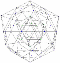
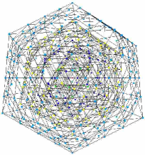
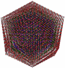
a)b)c)

Figure 2: a) IF75, b) IF509, and c) IF9483, where IF = IC$\bigcup$FC.

It is probable that methods with a good background on the knowledge of the problem and using adaptive search, simulated annealing, lattices, basin hopping, funnels, phenotypes, fusion, evolutionary, and genetic operations have advantages over other methods because they are exploring the discrete search spaces of my lattice IF (hereafter only IF, see Figs. 2, and 3). It was stated by Northby [17]:

”The complexity of the problem lies in the fact that while it is always possible with a computer to allow a particular initial configuration to relax to the adjacent minimum of the potential energy surface, unless the starting configuration has been chosen to lie in the proper valley, or ”catchment basin, the resulting configuration will not correspond to the absolute minimum.”

Considering this remark, the mentioned methods can relax efficiently but the global minimum could escape from the initial selection in a particular lattice, making necessary the exhaustive creation of good initial clusters from different lattices or the transformation in good ones before the relaxation. Some successful methods use random selection of clusters and particles in a random way from the well know lattices type IC, FC, ID, TO and so on. Here, my propositions close the gap stated by Northby between the initial configuration and the global minimum cluster, in the sense that exist a lattice or a set as an appropriate search space from where it is possible to repeat all the putative optimal LJ clusters reported in The Cambridge Cluster Database (CCD) [26]. As an example, a lattice and a set are presented, IF9483 and MIF1739 respectively, such that they contain particular clusters that match with the putative optimal LJ clusters from $n=2,\ldots,100$ in one relaxation (minimization procedure). The complexity of this type of telephone directory method on IF is at most $O(n^{3})$ (the complexity of the relaxation multiplying by the complexity of the evaluation of a pair potential function for $n$ particles). However, this is not a lower bound for the complexity of discrete methods of SOC using IF. There are cases where it is possible to reduce the numbers of operations in the evaluation of the potential of a cluster by the symmetry inherited from IF. $C_{13}^{\ast}$ is an example where the cost of computing the potential is 4 instead of 91 operations (section 4.1 depicts this). IF allows to have automatic classification of clusters, a measurement in term of the number of adjustment for solving SOC in discrete fashion, and let to study NP complexity.

IF (as a discrete search space) coincides with the well know result from Quantum Mechanic that the particles interact in discrete fashion. Moreover, the existence of particles forming an IF can be seeing as particles in a hot temperature where the positions IC and FC could be occupied with equal likelihood. What it makes difficult to predict the geometric shape of small clusters is the mobility of the potential energy surface (PES). PES changes from small cluster to larger ones in the sense that the displacement of a particle in the outer shell from its lattice’s position has more free in the small clusters than in large ones in order to reduce the total cluster energy. On the other hand, for large clusters the transition to stable structures corresponds to a change of geometrical structure from IC to a decahedral lattice [13, 23] where the PES has less freedom. Section 6 has Figures where the normalized gradient is depicted. From these figures the PES’s mobility for the particles in the outer shells of a small cluster can be explained.

The notation and some conventions used in this report are given in Section 2. Section 3 describes the properties of the potential where this methodology can be applied. Sections 4 and 5 describe the special IF9483, MIF1739 and methods for them. Section 6 presents MIF1739. It contains all the putative optimal LJ clusters, tables LABEL:tb:On_off_0-LABEL:tb:On_off_32 give in an efficient and short notation all the indices to build the initial clusters, tables LABEL:tb:Changes_0-LABEL:tb:Changes_9 present the geometrical type, the initial and minimum LJ potential, and a measure of the adjustment necessary to transform from $C_{n+1}$ to $C_{n}$, and tables LABEL:tb:idMinLattice_0-LABEL:tb:idMinLattice_15 give the coordinates of MIF1739 in order to reproduce the numerical results presented here. In addition, this section includes novel figures of the difficult clusters inside of IF9483, and novel descriptions of some clusters. Finally, Section 7 presents my conclusions and future work.

2 Notation

$\mathbb{N}$ is the set of the natural numbers, $\mathbb{Q}$ is the set of the rational numbers, and $\mathbb{R}$ is the set of the real numbers.

A lattice, $\Omega=\left\{p_{i}\right\}_{i\in\text{I}}$, $p_{i}\in\mathbb{R}^{3}\forall i\in$I where I is a set of indexes (I=$\mathbb{R}$ or I=$\mathbb{N})$ is a set of points in a regular pattern in $\mathbb{R}^{3}$.

A cluster of size $n$ is $C_{n}=\left\{p_{i_{{}_{1}}},p_{i_{2}},...,p_{{}_{i_{n}}}\right\}$, $p_{i_{j}}\in\Omega$, $\forall j=1,\ldots,n$.

$\overrightarrow{\cdot}:L\rightarrow\mathbb{R}^{3\cdot}$ means $\overrightarrow{\cdot}\left(C_{n}\right)=\overrightarrow{C}_{n}$ $=$ $\left(p_{i_{{}_{1}}},p_{i_{2}},...,p_{{}_{i_{N}}}\right)\in\mathbb{R}^{3N}$, it is a vector representation of a cluster where $p_{i_{l}}=(x_{i_{l}},y_{i_{l}},z_{i_{l}})$ is mapped into cylindrical coordinates $(\rho_{i_{l}},\alpha_{i_{l}},\beta_{i_{l}})$, $\rho_{i_{l}}\in\mathbb{R}^{+}$, $\alpha_{i_{l}}\in[0,\pi]$ is zero on the semi-axes $Y^{+}$ and the $\theta_{i_{l}}\in[0,2\pi]$. Then coordinates $p_{i_{{}_{l}}}\leq p_{i_{m}}$, $l\leq m$ if $\rho_{i_{l}}\leq\rho_{i_{n}}$; or if $\rho_{i_{l}}=\rho_{i_{n}}$ and $\alpha_{i_{l}}\leq\alpha_{i_{m}}$; or if $\rho_{i_{l}}=\rho_{i_{n}}$, $\alpha_{i_{l}}=\alpha_{i_{m}}$, and $\beta_{i_{l}}\leq\beta_{i_{m}}$.

$\overrightarrow{C}_{n}$ is used as an element of the metric space $\mathbb{R}^{3n}$.

Let $p_{j}$, $p_{k}\in\mathbb{R}^{3}$ and $r_{j,k}$ = $\sqrt{\left(x_{j}-x_{k}\right)^{2}+\left(y_{j}-y_{k}\right)^{2}+\left(z_{j}-z_{k}\right)^{2}}$. Some potential functions [16] are

Buckingham Potential (BU):

$$\hbox{VBU}_{i,j}=\alpha_{i,,j}e^{\beta_{i,,j}r_{i,,j}}+\frac{\gamma_{i,,j}}{r_{i,,j}^{6}}$$

where $\alpha_{i,j}$, $\beta_{i,j}$, and $\gamma_{i,j}$ are parameters for the type of particles.

Kihara Potential (KI):

$$\hbox{VKI}_{i,j}=4\epsilon_{0}\left[\left(\frac{1-\gamma}{r_{i,,j}/\sigma-\gamma}\right)^{12}+\left(\frac{1-\gamma}{r_{i,,j}/\sigma-\gamma}\right)^{6}\right]$$

where $\epsilon_{0}$, $\sigma$, and $\gamma$ are parameters for the type of particles.

Lennard-Jones potential (LJ):

$$\hbox{VLJ}_{i,j}=V_{i,j}=4\epsilon_{0}\left[\left(\frac{\sigma_{i,j}}{r_{i,j}}\right)^{12}-\left(\frac{\sigma_{i,j}}{r_{i,j}}\right)^{6}\right]$$

where $\epsilon_{0}$ and $\sigma_{i,j}$ are parameters for the type of particles. For the examples in this paper, $\epsilon_{0}=\sigma_{i,j}=1$.

Morse Potential (MO) [9] is

$$\hbox{VMO}_{i,j}=\left(1-e^{-\alpha\left(1-r_{i,j}\right)}\right)^{2}-1$$

where $\alpha$ is a parameter.

A pair potential can represented by

$$\hbox{VXX}_{j,k}=EXX\left(\left\{p_{j},p_{k}\right\}\right)=EXX(p_{j},p_{k})=EXX(r_{j,k})$$

where XX can be BU for Buckingham, KI for Kihara, LJ for Lennard-Jones, and MO for Morse Potentials.

The complete potential of a cluster is

$$\hbox{EXX}\left(C_{n}\right)=\sum_{i=1}^{n-1}\sum_{j=i+1}^{n}\hbox{VXX}_{j,k}$$

The Lennard-Jones Potential (LJ) is written also as

$$\hbox{E}\left(C_{n}\right)=E\left(\overrightarrow{C}_{n}\right)=4\sum_{i=1}^{n-1}\sum_{j=i+1}^{n}(\frac{1}{r_{jk}^{12}}-\frac{1}{r_{jk}^{6}})$$

when there is not confusion with the other potentials.

The conventions follows in the paper for the problems are:

• SOC denotes the problem of search of optimal clusters.

• SOCC denotes SOC solved in a continuous search space.

• SOCD denotes SOC solved in a discrete search space. Here it is assumed that an appropriate discrete set or lattice of points in $\mathbb{R}^{3}$ exists.

• SOC($n$) denotes SOC for clusters of size $n$.

• SOCC($n$) denotes SOCC for clusters of size $n$.

• SOCD($n$) denotes SOCD for clusters of size $n$.

• SOCYXX denotes one of the previous problems, where Y=C or Y=D, and XX is BU, KI, LJ, and MO Potentials.

• SOCYXX($n$) denotes one of the previous problems for clusters of size $n$.

For $n\in\mathbb{N}$, $n\geq 2$ SOCCXX($n$) can be stated:

Given $A\subset\mathbb{R}^{3}$, look for $\overrightarrow{C}_{n}^{\ast}=(x_{1},\ldots,x_{n})\in\mathcal{A}^{n}$ such that EXX$\left(\overrightarrow{C}_{n}^{\ast}\right)$ $\leq$ EXX$\left(x\right),\forall x\in A^{n}$ where $A^{n}=A\times\cdots\times A$ (n times).

In similar way SOCDXX($n$) can be stated:

Given a lattice $\Omega=${$p_{i}$ $|$ $p_{i}\in\mathbb{R}^{3}$, $i=1,\ldots,N$ $N\gg n$, $N\in\mathbb{N}$}, find $\overrightarrow{C}_{n}^{\ast}=(p_{l_{1}},\ldots,p_{l_{n}}),$ such that EXX$\left(\overrightarrow{C}_{n}^{\ast}\right)$ $\leq$ EXX$\left(\overrightarrow{C}_{I^{k}}\right)$, $\forall I^{k}\subset\mathbb{N}$, $|I^{k}|=n$ where $\left|\cdot\right|$ is the number of elements of a set. This means EXX$\left(\overrightarrow{C}_{n}^{\ast}\right)$ is less or equal than the potential of any other cluster of $n$ points from $\Omega$.

The function adjust is defined as Adj:$2^{\Omega}\times 2^{\Omega}\rightarrow\mathbb{N}$, Adj$\left(C_{n}\text{, }C_{m}\right)$ = $\left|\left(C_{n}\setminus C_{m}\right)\cup\left(C_{m}\setminus C_{n}\right)\right|$.

The function On is defined as On:$2^{\Omega}\times 2^{\Omega}\rightarrow\mathbb{N}$, On$\left(C_{n}\text{, }C_{m}\right)$=$\left|C_{m}\setminus C_{n}\right|$.

The function Off is defined as Off:$2^{\Omega}\times 2^{\Omega}\rightarrow\mathbb{N}$, Off$\left(C_{n}\text{, }C_{m}\right)$=$\left|C_{n}\setminus C_{m}\right|$.

It is easy to see that Adj$\left(C_{n}\text{, }C_{m}\right)$ = On$\left(C_{n}\text{, }C_{m}\right)$ + Off$\left(C_{n}\text{, }C_{m}\right)$.

There are several references that explains how to build IC and FC [15, 30, 24], in particular Northby [17] called to the combination of both IF. Hereafter, IC$n$ represent a subset of $n$ points of type IC, and similarly for FC and IF.

$C_{j}$ $\rightarrow C_{j}^{\ast}$ means $C_{j}^{\ast}=\min$($C_{j}$) under some potential function and where $\min$ is a minimization procedure. The results reported here were computed with a version the Conjugated Gradient Method (CGM). Also, in the text when there is not confusion $C_{j}^{\ast}$ means the putative optimal LJ cluster.

In some figures the normalized gradient of LJ is depicted. This vector correspond to $\nabla$ VXX $(x^{\ast})$ / $\|$ $\nabla$ VXX ($x^{\ast}$) $\|$. The corresponding component of the gradient is drawn as a vector in $\mathbb{R}^{3}$ on each particle of a given cluster.

3 Properties of the LJ Potential

Note that LJ, BU, and KI but MO Potentials share the well potential’s properties [18]:

1. $\lim_{r\rightarrow r_{0}}\hbox{VXX}\left(r\right)=\infty$

2. Each cluster under a pair potential has a basin.

Moreover in one dimension, given two particles, the first is fixed on $(0,0,0)$, and the second with coordinates $(r,0,0)$ is free to move on axes X. The following properties are satisfied for E (similar results are given by Xue [32]):

1. E$\left(r\right)=4(\frac{1}{r^{12}}-\frac{1}{r^{6}}).$

2. E${}^{\prime}\left(r\right)=\allowbreak 24\frac{-2+r^{6}}{r^{13}}$

3. E${}^{\prime\prime}\left(r\right)=\allowbreak-24\frac{-26+7r^{6}}{r^{14}}$

4. E$\left(r\right)<0$, $r>1$, $\lim_{r\rightarrow\infty}\hbox{E}\left(r\right)=\allowbreak 0.$

5. $r^{\ast}=\sqrt[6]{2}$, is the global minimum of E. E$\left(r^{\ast}\right)=\allowbreak-1.0,$ E${}^{\prime}\left(r^{\ast}\right)=\allowbreak 0$ E${}^{\prime\prime}\left(r^{\ast}\right)>0$

6. E$\left(r^{\ast}+\xi\right)\approx-1+O\left(\xi^{2}\right),0\leq\left|\xi\right|<<1.$ By a series expansion E$\left(r^{\ast}+\xi\right)=4\left(\frac{1}{\left(\sqrt[6]{2}+\xi\right)^{12}}-\frac{1}{\left(\sqrt[6]{2}+\xi\right)^{6}}\right)=-1+\left(18\left(\sqrt[3]{2}\right)^{2}\right)\xi^{2}+O\left(\xi^{3}\right)$, with $0\leq\left|\xi\right|<<1,$ E$\left(\sqrt[6]{2}+\xi\right)\approx-1+K\xi^{2},K=18\left(\sqrt[3]{2}\right)^{2}.$

7. The basin region of E is the interval $\left(1.053666\,8,1.\,2444551\right)$. E${}^{\prime\prime}\left(r\right)>0$, $\forall r\in\left(1.053666\,8,1.\,2444551\right)$. Therefore E$\left(r\right)$ is convex and E$\left(r\right)<-0.786\,982\,15$, $\forall r\in\left(1.053666\,8,1.\,2444551\right)$.

Figure 1 depicts E$\left(r\right)$, E${}^{\prime}(r),$ and E${}^{\prime\prime}\left(r\right)$ in $\left(1.053666\,8,1.\,2444551\right)$.

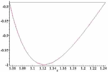
a)

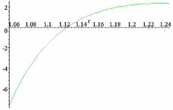
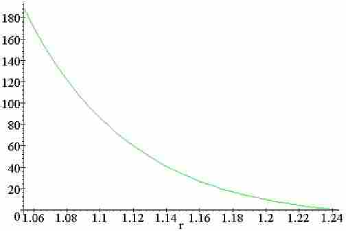
b) c)

Figure 1: a) E$(r)$, b) E${\prime}(r)$, and c) E${\prime\prime}(r)$.

4 Unified Lattice

This section explains what is the relationship between the discrete and continuous SOC. The main proposition is: Exist a discrete set for all optimal clusters where their potential has the same value as in the solution of the continuous search of optimal clusters. This type of potential function must fulfill the conditions of a well potential [18]:

1. Potential function creates a infinite repulsion force when distance between two particles goes to 0.

2. Each cluster under this potential has a basin.

Note that BU and LJ functions comply 1. KI function and MO function do not comply with 1.

Proposition 1.

Exist a discrete set, $\Omega$, where $\forall j\in N$, $j\geq 2$, the potential of SOCDXX($j$) has the same optimal value of SOCCXX($j$) for a potential function such that

1. $\lim_{r_{i,j}\rightarrow 0}\hbox{VXX}\left(r_{i,j}\right)=\infty$.

2. $\nabla^{2}\hbox{VXX}\left(x^{\ast}\right)$ semi-positive$,\left\|\nabla\hbox{VXX}\left(x^{\ast}\right)\right\|\ll 1$ and $\frac{\left\|\nabla\hbox{VXX}\left(x^{\ast}\right)\right\|}{\left|\hbox{VXX}\left(x^{\ast}\right)\right|}<\delta_{0}$, where $0<\delta_{0}\ll 1$

where XX is BU or LJ.

Proof.

Without lost of generality, I assume a continuous search for a cluster of size $j$ in A=$\{p=\left(x,y,z\right)$ $\in\mathbb{R}^{3}\ |\ \left\|p\right\|\leq r$}, a ball of ratio, r$\gg 0$ from where $\overrightarrow{\cdot}:$A$\rightarrow\mathbb{R}^{3j}$. The continuous search can be stated as generate $k$ random vectors $\left\{\overrightarrow{C}_{j}^{l}\right\}_{l=1,\ldots,k}$ with coordinates in A and using a minimization routine to compute $\overrightarrow{C}_{j}^{{}^{\ooalign{\hfil\raise 0.1507pt\hbox{$\scriptstyle\mathrm{\text{missing}}{R}$}\hfil\crcr\text{$\mathchar 525\relax$}}}l}=(x_{l_{1}},x_{l_{2}},\ldots,x_{l_{N}})$ such that the property 2 is fulfill. Then select $x^{\ast}$ $=$ $\overrightarrow{C}_{j}^{\ast}=\min_{l=1,\ldots,k}\left\{\overrightarrow{C}_{j}^{{}^{\ooalign{\hfil\raise 0.1507pt\hbox{$\scriptstyle\mathrm{\text{missing}}{R}$}\hfil\crcr\text{$\mathchar 525\relax$}}}l}\right\}=\left(x_{1}^{\ast},\ldots,x_{j}^{\ast}\right)$. Repeating this procedure, A is exhaustively explored, therefore this must provide a solution of SOCCXX($j$). This means, EXX$\left(x^{\ast}\right)$ $\leq$ EXX$\left(x\right),\forall x=(p_{1},\ldots,p_{j})\in\mathbb{R}^{3N}$, $p_{l}\in A$, $l=1,\ldots,j$ .

The first property does not allow to have $p_{m}=p_{n}$ with $m\neq n$. Therefore, $p_{i}$, $i=1,\ldots,j$ are separate points in A$\subset\mathbb{R}^{3}$. Moreover, we can translate and set $x_{1}$ $=$ $(0,0,0)$ without changing the value of EXX. Therefore $\exists\varepsilon_{0}>0$ for solving SOCCXX($j$) and there is not need of the points, $p\in\mathbb{R}^{3}$ such that $\left\|p\right\|<\varepsilon_{0}$ because they are never going to participate by the condition 1.

For other coordinates of $x^{\ast}$, the second property provides a basin or convexity region around it. A Taylor series for a potential function around of $x^{\ast}\in\mathbb{R}^{3j}$ for a direction $d\in\mathbb{R}^{3j}$ with $0<\varepsilon\ll 1$ is

$$\hbox{VXX}\left(x^{\ast}+\varepsilon d\right)=\hbox{VXX}\left(x^{\ast}\right)+\varepsilon d\cdot\nabla\hbox{VXX}\left(x^{\ast}\right)+\frac{1}{2}\varepsilon^{2}d\cdot\nabla^{2}\hbox{VXX}\left(x^{\ast}\right)\cdot d+O\left(\varepsilon^{3}\right).$$

By the convexity, $\frac{1}{2}\varepsilon^{2}d\cdot\nabla^{2}V\left(x^{\ast}\right)\cdot d\geq 0$. Therefore

$$\left|\hbox{VXX}\left(x^{\ast}+\varepsilon d\right)-\hbox{VXX}\left(x^{\ast}\right)\right|\leq\left|\varepsilon\right|\left\|d\right\|\left\|\nabla\hbox{VXX}\left(x^{\ast}\right)\right\|,$$

$$\frac{\left|\hbox{VXX}\left(x^{\ast}+\varepsilon d\right)-\hbox{VXX}\left(x^{\ast}\right)\right|}{\left|\hbox{VXX}\left(x^{\ast}\right)\right|}\leq\left|\varepsilon\delta_{0}\right|.$$

This property allows to select a truncated representation of $x^{\ast}$ for some $\varepsilon_{1}=\varepsilon\delta_{0}>0$. Therefore, $x=\left(p_{1},\ldots,p_{j}\right)\in\mathbb{R}^{3j}$ such that $\left\|x-x^{\ast}\right\|<\varepsilon_{1}$ and $\left\|p_{l}-p_{l}^{\ast}\right\|<\varepsilon_{0}$ $l=1,\ldots,j$ are not necessary to consider because they are never going to improve the potential of $x^{\ast}$. Let $\varepsilon_{j}=\min\left\{\varepsilon_{0},\varepsilon_{1}\right\}$.

Finally, $\Omega^{o}=\cup_{j=2}^{\infty}C_{j}^{\ast}$ for $\varepsilon^{\ast}=\min\left\{\varepsilon_{j}\right\}_{j=2}^{\infty}$ and by the construction of $\Omega^{o}$ it follows immediately that SOCDXX($j$) and SOCCXX($j$) have the same solution $\forall j\in\mathbb{N}$, $j\geq 2$.    

Remark 1.

In the previous proposition, A is a subset of $\mathbb{R}$. A has the cardinality of $\mathbb{R}$ but the proposition states that a discrete set of points of A is sufficient in order to have the same solution between SOCDXX($j$) and SOCCXX($j$) where XX is BU or LJ.

Proposition 2.

The set $\Omega^{l}$=$\{p_{i{{}_{j}}}$ $\in$ $C_{j}^{k}$ $|$ $C_{j}^{k}$ is a local optimal cluster, such that $C_{j}^{k}$ = $\{p_{i{{}_{j}}}\}$, ${i{{}_{j}}}\in I^{k}$, $|I^{k}|=j$} under a well potential function (a potential that fulfill the properties of the Proposition 1) is numerable.

Proof.

Let assume that the $\cup_{j=1,\ldots,N,|I^{k}|=j}C_{j}^{k},$ is not numerable. This means $\exists K_{j}=\cup_{|I^{k}|=j}I^{k}$ is not numerable. From the previous proposition, clusters can be created from the continuous search depicted in the previous proposition, therefore each one fulfill properties 1) and 2) and we add the coordinates of each $C_{j}$ founded to some $\Omega$. Then for $j,\ \exists\varepsilon_{j}$ such that $\overrightarrow{C}_{j}^{m},\overrightarrow{C}_{j}^{n}\in\mathbb{R}^{3j}$ and $\overrightarrow{C}_{j}^{m}\neq\overrightarrow{C}_{j}^{n}$ for $\forall m\neq n$, $m,n\in K_{j}$. But each $\overrightarrow{C}_{j}^{m}$ can be approximated $\underline{\overrightarrow{C}}_{j}^{m}\in\mathbb{Q}^{3j}$ if $\left\|\underline{\overrightarrow{C}}_{j}^{m}-\overrightarrow{C}_{j}^{m}\right\|<\varepsilon_{j}$ $\forall m\in K_{j}$, which imply that $\cup_{m\in K_{j}}\underline{C}_{j}^{m}\subset\mathbb{Q}^{3}$ is not numerable!    

Proposition 3.

The set $\Omega^{o}$=$\{p$ $\in$ $C_{j}^{\ast}$ $|$ $C_{j}^{\ast}$is the global optimal cluster $\forall$ $j\in\mathbb{N}$} is numerable.

Proof.

$\Omega^{o}$ is the union of finite set of points, therefore is numerable.    

Proposition 4.

The set $\Omega^{b}$=$\{p$ $\in$ $C_{j}^{k^{\prime}}$ $|$ $C_{j}^{k^{\prime}}$ is a cluster in a basin for the optimal local clusters $C_{j}^{k}$ of size $j$, $\forall$ $j$ $\in$ $\mathbb{N}$} is not numerable.

Proof.

Given an optimal local cluster $C_{j}^{k}$ by the condition 2 of Proposition 1, $\exists\delta_{0}>0$ and $d\in\mathbb{R}^{3j}$ such that $\forall$ 0 $\leq$ $\delta\leq\delta_{0}$ $\overrightarrow{C}_{j}^{k\delta}$ = $\overrightarrow{C}_{j}^{k}+\delta d$, then $\overrightarrow{C}_{j}^{k\delta}$ $\rightarrow$ $C_{j}^{k}$, $\forall$ 0 $\leq$ $\delta\leq\delta_{0}$. Therefore, $\Omega^{b}$ is union of non-numerable sets for each optimal local cluster.    

Proposition 5.

Exist a set, $\Omega^{\ast}$ such that $\exists$ $C_{k}^{{}^{\prime}}$ $\in$ $\Omega^{\ast}$, $C_{k}^{{}^{\prime}}$ $\rightarrow$ $C^{\ast}_{k}$ $\in$ $\Omega^{o}$ $\forall k\geq 2$.

Proof.

The results follows from $\Omega^{b}\bigcap\mathbb{Q}^{3}$ $\neq$ $\emptyset$.    

Remark 2.

The last proposition states that $\Omega^{\ast}$=$\Omega^{b}\bigcap\mathbb{Q}^{3}$ is one trivial set where $\exists$ $C_{j}$, such that $C_{j}\rightarrow C^{\ast}_{j}$, $\forall j\geq 2$. In order to find IF, I add each putative optimal LJ cluster, $C^{\ast}_{j}$, $j$=2,$\ldots$,1000. It was a surprise that taking $C_{13}^{\ast}$ and adjusting the other putative optimal LJ clusters to it, the IF structure show up naturally.

The next proposition states that is not possible to find a function from $\mathbb{N}$ to $\Omega$ capable to give all optimal clusters. Hereafter, $\Omega$ is a numerable set and could be $\Omega^{l}$ or $\Omega^{\ast}$.

Proposition 6.

$\nexists s:\mathbb{N}\rightarrow\Omega$, $s(j)=C_{j}=\left\{x_{i_{1}},\ldots,x_{i_{j}}\right\}$, $x_{i_{k}}\in\Omega$ $\forall k=1,\ldots,j$ such that $s\left(j\right)=C_{j}^{\ast},\forall j\in\mathbb{N}$.

Proof.

The proof is based in building a Cantor’s Diagonal schema. Suppose that such selection function, $s$, exists for some order in $\Omega$, which is numerable. Then changing the first particle in $\Omega$ that belong to the $C_{2}^{\ast}$ for any other different and far way from this one, the new order $\Omega_{2}$ is an order where $s$ can not give $C_{2}^{\ast}$. This procedure is repeated for $C_{k}^{\ast}$, $k=3,\ldots,\infty$ giving $\Omega_{k},$ $k=3,\ldots,\infty$ where $s$ can not give $C_{k}^{\ast}$. The set of points that belong to the diagonal differs from all the enumerations $\Omega_{k},$ $k=2,\ldots\infty$ which are all the possible enumerations of $\Omega$!    

Proposition 7.

It is not possible to find an algorithm with polynomial complexity to solve SOCD($j$), $\forall j$ $\in$ $\mathbb{N}$.

Proof.

If such algorithm exist, it means that it is possible to find $M\in\mathbb{N}$, $M>0$, $T(j)\leq O\left(j^{M}\right)\forall j\in\mathbb{N}$ where $T$ is the time to take this algorithm to find $C_{j}^{\ast}$. But this means that such algorithm is the function $s$ of the previous proposition!    

Remark 3.

The last proposition states that it is not possible to build a selection function in computational time for finding all the optimal clusters from $j\geq 2$, $j\in\mathbb{N}$. In particular, it states that the complexity of finding all the optimal clusters from $j=2,\ldots,\infty$ cannot be derived from some arbitrary inhered order of $\Omega$ (numerable).

One of the reason of the success of the methods for SOCCXX($j$) and SOCDXX($j$) is the combination of different lattices, which are subsets of $\Omega^{\ast}$. Moreover, from the cardinality point of view, $\Omega^{\ast}$ is a smaller set than $\mathbb{R}^{3}$, and it seems to be the right search space to explore the complexity of the NP problem SOCDXX($j$), $\forall j\geq 2.$

The Proposition 1 permits to build a discrete set of points after the solution of the SOCDXX($j$), $\forall j\geq 2$ and also proofs that exist a set where SOCC and SOCD have the same solution, therefore SOCC is not efficient way for SOC.

It was not easy to build a set of points as a discrete lattice from basin regions for solving SOCDLJ($j$), $\forall j\geq 2$ for the putative optimal clusters, i.e., a set of points in $\mathbb{R}^{3}$ with a regular structure. However, combining IC and FC with an appropriate separation was the surprising answer. Section 6 presents numerical experiment of the propositions of this section. Particularly, for SOCDLJ($j$) a lattice and a set, IF9483 and MIF1739, are presented with the property, $\exists C_{j}\rightarrow C_{j}^{\ast}$, $j=2,\ldots,1000$ in the sense that ELJ($C^{\ast}_{j}$) are the putative optimal potential LJ values from [26] or better ones.

4.1 Symmetry reduces the Complexity of Potential’s Evaluation

For SOC, the symmetry inhered from a lattice $\Omega^{\ast}$ can reduce the number of operations to evaluate a potential function. A simple example, taking $\Omega^{\ast}$= IF and $C_{13}$ as a centered icosahedron inside of a ball of ratio, $r^{\ast}=\sqrt[6]{2}$. Here, without lost of generality the points of $C_{13}=\left\{p_{1},\ldots,p_{13}\right\}$ are:
$p_{1}$ = (0.000000000000, 0.000000000000, 0.000000000000),
$p_{2}$ = (0.000000000000, 1.081838288553, 0.000000000000),
$p_{3}$ = (0.967625581547, 0.483812790773, 0.000000000000),
$p_{4}$ = (0.299012748890, 0.483812790773, -0.920266614664),
$p_{5}$ = (-0.782825539663, 0.483812790773, -0.568756046574),
$p_{6}$ = (5,-0.782825539663, 0.483812790773, 0.568756046574),
$p_{7}$ = (0.299012748890, 0.483812790773, 0.920266614664),
$p_{8}$ = (0.782825539663, -0.483812790773, -0.568756046574),
$p_{9}$ = (-0.299012748890, -0.483812790773, -0.920266614664),
$p_{10}$ = (-0.967625581547, -0.483812790773, 0.000000000000),
$p_{11}$ = (-0.299012748890, -0.483812790773, 0.920266614664),
$p_{12}$ = (0.782825539663, -0.483812790773, 0.568756046574), and
$p_{13}$ = (0.000000000000, -1.081838288553, 0.000000000000).

Then by the symmetry on these points, EXX$\left(C_{13}\right)$ =12VXX_1,2+30VXX_2,3+ 30VXX_2,8+ 6VXX_2,13

which requires five points {$p_{1}$, $p_{2}$, $p_{3}$, $p_{8}$, $p_{13}$} and the four factors $\hbox{VXX}_{1,2}$, $\hbox{VXX}_{2,3}$, $\hbox{VXX}_{2,8}$, and $\hbox{VXX}_{2,13}$ for any potential function. But without symmetry, EXX$\left(C_{13}\right)=$ $\sum_{i=0}^{n-1}\sum_{j=i+1}^{13}\hbox{VXX}{i,j}$ needs thirteen points and $13(13+1)/2=91$ factors $\hbox{VXX}_{i,j}$. In particular for this cluster ELJ($C_{13}$) = -44.326801 = ELJ($C^{\ast}_{13}$).

5 Methods for IF

There are several references that explains how to build IC and FC [13, 15, 24, 30]. I build an IF for the Lennard-Jones Potential using the propositions of the previous section. The first approach was to use Proposition 1 to build a set from the $C_{j}^{\ast}$, $j=2,\ldots,1000$ by adding in growing order the points of each $C_{j}^{\ast}$ but after few numerical experiments, a fixed combination of an IC and an FC together with an step ratio, $r^{\ast}=1.08183839$, between shells makes possible to build an IF such that $\exists C_{j}$ $\rightarrow C_{j}^{\ast}$ using a minimization procedure based on the CGM. The possibility to find a lattice was predicted by Proposition 5. The value $r^{\ast}$ correspond to the icosahedron described in section 4.1. In addition, this is the only cluster where SOCDLJ(13) does not need a relaxation, moreover, ELJ($C_{13})=ELJ(C_{13}^{\ast}$). Note that the particular order of the sequence of points is very important to reproduce the putative optimal LJ clusters, therefore tables LABEL:tb:idMinLattice_0-LABEL:tb:idMinLattice_15 give all the coordinates of MIF1739.

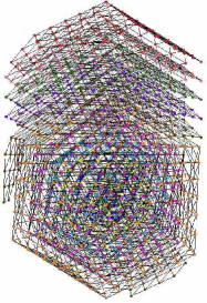
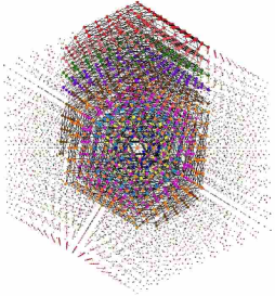
a) b)

Figure 3: a) MIF1739 and b) MIF1739 inside of IF9483. MIF1739 and IF9483 contain $C_{n}$, such that $C^{*}_{n}$ = $\min$($C_{n}$) $n=2,\ldots,1000$.

Give the result in IF9483 is lengthy but with MIF1739 is a short way to present it. Meanwhile MIF1739 contains only 1739 points, the complete IF with the same property needs 9443 points. The number of points of the IF9483 comes from sum of the magic numbers of the particles of the complete shells IC and FC for the shells 0 to 11. Figure 2 depicts IF75, IF509, and IF9483. Figure 3 depicts MIF1739 alone and inside of an IF9483.

The construction of the MIF1739 is done by the following algorithm:

• $C_{1000}^{{}^{\prime}}$ is a rotation of $C_{1000}$ to set as many particles as possible of the last shell over the semi-axes $Y^{+}$.

• for j=999, 2

• $C_{j}^{\prime}=\min$Adj$\left(C_{j+1}^{{}^{\prime}}\text{, }C_{j}\right)$ over all rotations of $C_{j}$ based on the symmetry of the centered icosahedron in

• IF.

• end for

• MIF=$\cup_{j=2,\ldots,1000}C_{j}^{\prime}$

Remark 4.

In the step 3, for the clusters that are not centered IC or FC as the $C_{38}^{\ast}$, $C_{98}^{\ast}$ and the Ino’s decahedrons the rotation are five and they are around of the axes $Y$. In addition, these clusters exist on infinity positions of an infinite IF, therefore they were manually translated to closed position toward the center of IF and over the semi-axes $Y^{+}$.

The tables LABEL:tb:On_off_0-LABEL:tb:On_off_32 allow to build all the $C_{j}^{\ast}$ from MIF1739. The algorithm is

• $C_{1000}$={$p_{i}\in$ MIF1739 $|$ $i$ is in the column On in tables LABEL:tb:On_off_0-LABEL:tb:On_off_32 for $C_{1000}$}.

• $C_{1000}^{\ast}=$ $\min$($C_{1000}$).

• for j=999 to 2

• $C_{j}$=$C_{j+1}\setminus${$p_{i}\in$MIF1739 $|$ $i$ is in the column Off in tables LABEL:tb:On_off_0-LABEL:tb:On_off_32 for $C_{j}\}\cup$ {$p_{i}\in$MIF $|$ $i$ is in the column

• On in tables LABEL:tb:On_off_0-LABEL:tb:On_off_32 for $C_{j}\}\cup$ {$p_{i}\in$MIF $|$ $i$ is in the column On in tables LABEL:tb:On_off_0-LABEL:tb:On_off_32 for $C_{j}$}

• $C_{j}^{\ast}=$ $\min$($C_{j}$).

• end for.

The tables LABEL:tb:Changes_0-LABEL:tb:Changes_9 give the type of the putative optimal LJ clusters in IF as: 1=IC, 2=Ino’s decahedron (ID), 3= truncated octahedron (TO), and 5=FC; the initial, optimal and difference of LJ, and the value of Adj$\left(C_{j+1}^{{}^{\prime}}\text{, }C_{j}\right)$.

The classification of cluster is done automatically by identified the particles of a cluster with the type of particles of MIF1739, type is IC when all the particles of a cluster are only IC around the center of IF, type is ID if there is a particle in the cluster close to the center of mass of the cluster, such that it is on the semi-axes $Y^{+}$, type is TO when all particles are IC and they are inside of a tetrahedron formed by three internal axis of the IF, type is FC when at least one particle of the cluster is FC.

5.1 Methods for search in IF

The classification of the algorithms for SOC has many different approaches [27]. Here tree classes are depicted on a scale from comparisons versus properties (necessary and sufficient conditions of a problem):

Exhaustive Algorithm

It explores a search space of a problem verifying that the global optimum is founded. Here, for the comparisons an objective function is used to provide the way to determine the optimum. For small discrete and continuous problems, the algorithm’s complexity is not an issue. There are many global optimization methods that work fine for low dimension problems. By example, the classical Grid Method divides the search space in small boxes. Therefore, it can locate the global minimum by an exhaustive search. Generally, the complexity grows rapidly, exponentially and for the NP problems, there is not hope that exist a polynomial complexity algorithm.

Scout Algorithm

It is a fact widely accepted that using previous knowledge and natural (Physical, Chemical, Thermodynamical, Biological, Medical, and so on) understanding of the process and phenomena involved in a problem will help to design an efficient method. Here, some authors argue about how much and what type of knowledge could be used. Other authors apply the rule: ”Achievements kill doubt”. From a practical point of view, this category contains algorithms that can use all or a part of whatever is available. Most of the methods for clusters optimization belong to this category. A method in this category could find a novel solution without a guarantee of optimality. Most of the justifications for algorithm’s efficiency are done by numerical experiments on a set of problems (benchmark). This type of analysis depends on the researcher and his/her particular computers and working conditions. Therefore, a claim that SOC can be done in polynomial time O($n^{3}$) is a very strong statement. If this could be extended and proved then the NP problems will be class P! Exploring IF is like a travel in one axes of the IF towards axes Y⁺. MIF1739 is also the minimum region to explore without to many repetitions caused by the icosahedral symmetry.

Wizard Algorithm

There are problems where necessary and sufficient optimal conditions can be established for the solution. Generally these methods are efficient and they do not need to do exhaustive comparisons. By example, an optimization problem with a convex function can be efficiently solved by the Conjugate Gradient method or by the large family of Newton and Quasi-Newton methods.

In [1] the Peeling Method was presented. This method is similar to the algorithm 4.1 of Maier et al. [15]. It executes a greedy strategy to set Off the particles on the outer shell of a cluster and to set On particles inside of a lattice that are neighbor of the previous ones. In this way, an small change is done and a minimization routine computes the potential of this cluster. The Modified Peeling Method has three basic operations: forward, backward, itself. Moreover, the basic idea is to adjust a cluster by turning on a neighbor particle and turning Off a particle in the outer shell of a cluster or the centered particle. The complexity of each operation is $O($n${}^{3})$ for a forward ($C_{n}$ to $C_{n+1}$) and backward ($C_{n}$ to$C_{n-1}$), and $O($n${}^{4})$ for itself. These operations are quite similar to the proposed pivot algorithm [31], reverse greedy operator by Leary [13], the ”final repair” step of Hartke [8], Fusion Process by adding one particle to C_n of Solov’yov et al. [24], and the greedy search method [29] but the novelty is that in right search space this Modified Peeling Method is capable to find new solutions or reproduce the existent ones.

Given $C_{n}=\left\{p_{i_{1}},p_{i_{2}},...,p_{i_{n}}\right\}$, $p_{i_{j}}\in$ IF, $\forall j=1,\ldots,n$, computes the sets:

• $K_{C}$ = { $i_{k}$ $|$ $i_{k}$ such that $\exists p_{i_{k}}\in C_{n}$, $\exists p_{i_{l}}\in\hbox{\ IF\ }\setminus C_{n}$, where $p_{i_{k}}$ and $p_{i_{l}}$ are neighbors or $i_{l}=0$ (centered particle of $C_{n}$)}.

• $K_{\hbox{IF}}$ = {$i_{l}$ $|$ $i_{l}$ such that $\exists p_{i_{k}}\in C_{n}$, $p_{i_{l}}\in\hbox{\ IF\ }\setminus C_{n}$, where $p_{i_{k}}$ and $p_{i_{l}}$ are neighbors}.

The Modified Peeling Method executes this three operations:

• $C^{\ast}_{n+1}$ = $\min_{\hbox{set On\ }j\in K_{\hbox{IF}}}$ { $p_{j}$ } $\bigcup$ $C_{n}$ }.

• $C^{\ast}_{n-1}$ = $\min_{\hbox{set Off \ }k\in K_{C}}$ $C_{n}\setminus\{p_{k}$ }.

• $C^{\ast}_{n}$ = $\min_{\hbox{set Off\ }k\in K_{C}\hbox{, set On\ }j\in K_{\hbox{IF}}}$ $C_{n}\setminus\{p_{k}$ } $\bigcup$ { $p_{j}$ }.

Remark 5.

These operations do not guarantee global optimality.

For SOCD, it seems that a wise algorithm only could exist after founded the optimal clusters. One of the reason is that the global optimality is an open question for clusters with more than five particles [27]. The efficient method after founded the optimal cluster is a telephone directory method. This type of method uses a table with the data needed. The only operation is retrieving an entry of the table by an index, i.e., given the indexed table $(t[1],\ldots,t[K])$, $K\in\mathbb{N}$, $K>0$ and $j\in[1,K]$ then retrieve $t[j]$.

Proposition 8.

The telephone directory method in $\Omega^{o}$ (see Proposition 2) has complexity $O(1)$.

Proof.

Here, the only operation is to select the points of $\Omega^{o}$ from a table with the collection of the indexes of each optimal cluster. Therefore the complexity is only one operation.    

Remark 6.

$\Omega^{o}$ is not symmetric because the PES of small clusters. If the function $s$ of the Proposition 6 exists, its complexity would be one!

Proposition 9.

The telephone directory method on $\Omega^{\ast}$, and particularly on IF has complexity $O(n^{3})$.

Proof.

This limit comes from the complexity of the relaxation multiplying by the complexity of the evaluation of a pair potential function for $n$ particles. It is well know that the a minimization method as the CGM converges in at most the number of variables of the problem, which in this case is $3n$ and the worst case for evaluation of the potential is $O(n^{2})$.    

For space consideration, a table of the optimal clusters for a telephone directory method is not given. However, this table can be obtained from the tables LABEL:tb:On_off_0-LABEL:tb:On_off_32. The algorithm for the telephone directory method on this table is:

• $C_{n}$={ $p_{i}\in$ MIF1739 $|$ $i$ is in the column On in the telephone table of optimal clusters }.

• $C_{n}^{\ast}=$ $\min$($C_{n}$).

Remark 7.

The telephone directory method with MIF1739 or IF9483 has polynomial complexity $O(n^{3})$ for SOCD($n$). An estimation of complexity less than $O(n^{3})$ by other authors is probably biased by the particular data and environment of their numerical experiments. It is possible that this small difference was influenced by the data over the number of iterative steps of the relaxation or minimization procedure on a very good initial population of clusters, which is highly possible if an algorithm gets initial random clusters from IC, ID, and FC lattices.

The results presented in the next Section show that optimal clusters are not always around on the same localization in IF. Therefore exploring IF by Exhaustive Algorithms is hard and it has exponential complexity caused by the combinations of possible particles.

Proposition 10.

The function Adj is not bounded.

Proof.

Let assume that $\exists M>0$ such that Adj$(C_{n}$, $C_{m})$ $<M$ $\forall n,m\geq 2$. This means that for $m\gg M$ because the number of adjust is bounded, the complexity of founding SOCD($m$) from SOCD($m-1$) or from SOCD($m+1$) is $O(m^{2})$ which imply the existence of the function $s$ of Proposition 6.    

Remark 8.

Also, if Adj is bounded, the complexity of a telephone directory method in an sufficient large appropriate lattice IF or set $\Omega^{l}$ (see Proposition 2) is greater than $O(m^{2})$, the complexity of SOCD($m$) for large clusters, which is also impossible, moreover then SOCD is not NP!

Adding previous knowledge to build an scout algorithm is seemed to be the way to address SOCD, and the complexity can be decreased by symmetry. However, it easy to see that exists a cluster where symmetry cannot reduce the worst case of the complete pair potential’s evaluation for some clusters, which is $O(n^{2})$. Finally, by the Proposition 9, $O(n^{3})$ is a lower limit of the complexity of SOCD($n$) in IF.

6 Results

MIF1739 is a discrete lattice for LJ where $\exists$ $C_{n}$, such that $C_{n}^{\ast}$ = $\min(C_{n})$ under LJ and $C_{n}^{\ast}$ is the putative optimal cluster for $n=2,\ldots,1000$. I took the data from CCD [26] to verify that my results. Data for $C_{n}^{\ast}$ $n=148,\ldots,309$ came from Romero, Barrón, and Gómez [20] and data for $C_{n}^{\ast}$, $n=310,\ldots,1000$ came from the recently results of Shao et al. [30, 29]. I was able to repeat and even improve some of the putative optimal LJ clusters. From this comparison new putative optimal LJ clusters are $C_{537}^{\ast}$, $C_{542}^{\ast}$, $C_{543}^{\ast}$, $C_{546}^{\ast}$, $C_{547}^{\ast}$, $C_{548}^{\ast}$, $C_{664}^{\ast}$, and $C_{813}^{\ast}$. The particular interest are the $C_{542}^{\ast}$, $C_{543}^{\ast}$, $C_{546}^{\ast}$, $C_{547}^{\ast}$, and $C_{548}^{\ast}$ because to my knowledge they are first optimal LJ clusters type IC with central vacancy (CV) reported in the shell 310-561. The prediction of CV was stated in [22] for the next shell, 562-923. Table 1 summarizes these new results.

n $E^{\text{new}\ast}$ $E^{\text{old}\ast}$ $E^{\text{new}\ast}-E^{\text{old}\ast}$ T 537 -3659.52825 -3659.70629 -0.17804 1 542 -3698.95403 -3699.22727 -0.27324 1/CV 543 -3706.94784 -3708.21090 -1.26306 1/CV 546 -3730.50408 -3730.69222 -0.18814 1/CV 547 -3738.38788 -3738.68065 -0.29277 1/CV 548 -3746.37071 -3747.67942 -1.30871 1/CV 664 -4596.1978 -4596.1971 -0.0007 2 813 -5712.2517 -5712.2506 -0.0011 1

Table 1: Novel $C^{*}_{n}$.

What is easy to accept from our classification is that a cluster type ID is contained on any of the twelve axis of symmetry of IF (here the clusters type ID are on the semi-axes Y⁺), a cluster type TO is in a centered tetrahedron formed by the center and three axis of symmetry forming four triangular faces. One controversial result of this automatic classification is the cluster’s type for $C_{98}^{\ast}$, moreover, this is the only cluster in MIF1739 where the adjacency matrix [9] is not the same between $C_{98}$ and $C_{98}^{\ast}$, however, $C_{98}^{\ast}=\min$($C_{98})$. The right type of $C_{98}^{\ast}$ is tetrahedral (depicted by Leary [14]). The different type reported here comes from the distance between $C_{98}$ and $C_{98}^{\ast}$ but it is a fact that the basin around $C_{98}^{\ast}$ attracts this $C_{98}$ of type FC. Figures 8 and 9 depict novel views of $C_{98}$ and $C_{98}^{\ast}$.

Figure 7 a) depicts $C_{664}$ inside of IF9483 and b) depicts $C_{664}^{\ast}$ as ID.

Wales and Doye [25] have been used basin for search of optimal LJ clusters and get through the barrier of the PES caused be the deformation of the particles on the surface. Figure 6 b) gives another perspective of this. Because, $C_{37}^{\ast}$ and C${}_{39}^{\ast}$ are close to the center of IF, $C_{38}^{\ast}$  is a jump from the center of IF to the first truncated octahedron in one of the tetrahedron formed by three axes of symmetry of IF. From table LABEL:tb:On_off_32, the indices of the particles for these three clusters show that they do not share any particle. This is the unique case in the results where there is not intersection between three consecutive clusters. Figure 6 a) depicts $C_{38}^{\ast}$ with gradient, where $\left\|\nabla\hbox{VXX}\left(x^{\ast}\right)\right\|\thicksim$3.7$\cdot$10^-6. The gradient looks big by the normalization. The gradient of $C_{38}^{\ast}$ shows that this cluster is stable and elastic in the sense that it can be deformed by $\alpha\nabla\hbox{VXX}\left(x^{\ast}\right)$ for some small values of $\alpha$ and with a minimization routine, the deformed $C_{38}$ will return to $C_{38}^{\ast}$. The gradient of the thirty-two particles in the outer shell point toward the center and the six particles of the inner octahedron shell point towards the square faces of the outer shell making this cluster stable to twisting deformations.

Figure 4 a) depicts $C_{55}^{\ast}$ with gradient. Here the gradient shows that the particles on the top of the outer shell can move to close positions around the semi-axes $Y^{+}$, in similar way for the bottom. The gradient of the particles in the inner icosahedron points in diametrical directions and if this effect is combined with an incomplete outer shell is possible to have great displacement of particles from their positions on IF and, also, a possible twisting and shrinking on the top or bottom cap of a cluster. Similar results can be seen from the gradient of $C_{147}^{\ast}$ depicted in figure 5 a).

The graphical representation of the gradient helped to design IF. Our selection of the shell’s step size is to have the corresponding component of the gradient for the particles IC and FC pointed towards $(0,0,0)$. Figures 4 b) and 5 b) depicted IF75 and IF227 with their gradient.

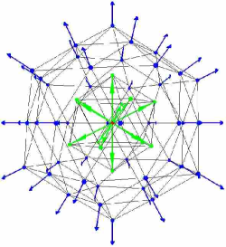
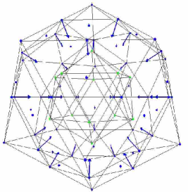
a) b)

Figure 4: a) $C^{*}_{55}$=IC$55^{*}$ and b) IF75 with gradient.

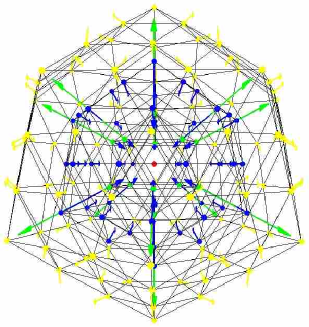
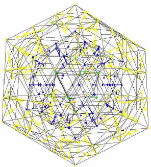
a) b)

Figure 5: a) $C^{*}_{1}47$=IC$147^{*}$ and b) IF227 with gradient.

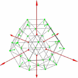
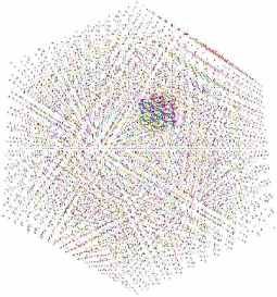
a) b)

Figure 6: a) $C^{*}_{38}$ with gradient and b) $C_{38}$ inside of IF9483.

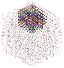
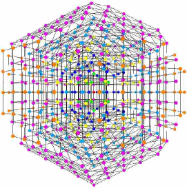
a) b)

Figure 7: a) $C_{664}$ inside of IF9483 and b) $C^{*}_{664}$.

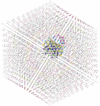
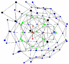
a) b)

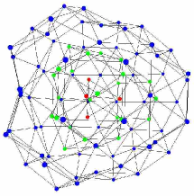
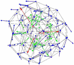
c) d)

Figure 8: a) $C_{98}$ inside of IF9483, b) $C_{98}$, c) $C^{*}_{98}$, and d) $C^{*}_{98}$ with gradient.

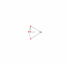
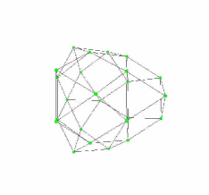
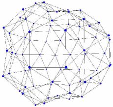
a)b) c)

Figure 9: Novel views of tetrahedral shells of $C^{*}_{98}$ a) interior shell with 4 particles, b) medium shell with 24, and c) outer shell with 70 particles.

7 Conclusions and future work

All the details of the construction of the IF9483 and MIF1739 are not given here but in a later article. Our first option was to build only $\Omega^{o}$ from Propositions1 and 3 but it was not as regular and symmetrical as IF. IF was the lattice that close the gap of Northby’s statement [17] in a regular, elegant and symmetrical lattice but hot. It seems that Proposition 1 is focus in build arbitrary sets from arbitrary points, that can be obtained from the separable points of $\mathbb{R}^{3}$ under BU or LJ. However, IF came naturally from using the $C_{13}^{\ast}$ as the seed. Of course, there could be other sets or lattices without such motifs but IF joints in one framework the well know IC and FC and all the putative optimal LJ clusters. Also, in the sets $\Omega^{l}$ and $\Omega^{o}$ of the Propositions 2 and  3 are not necessary a minimization procedure for any cluster. This gives a witness property for the optimality verification in the neighborhood of a cluster in polynomial time. Depicting the components of the gradient of the potential on each particle helps to understand the deformation of the PES for small clusters, but it need further study. Propositions 1, 2, and 3 permit see SOCDXX as the Traveling Salesman Problem in $\Omega^{l}$ or $\Omega^{o}$ and let to have a framework to analyze the complexity of SOCDXX where XX is BU or LJ. An open question is: Are there similar results for Kihara or Morse Potentials? Here the obstacle is that there is not strong rejection when $r\rightarrow 0$ and this does not allow to have separate points. Moreover: Is $C_{13}^{\ast}$ the global minimum? In my opinion it will be possible to answer this by a combination of an exhaustive search and by the symmetrical properties of IF and such proposition could be proved by using a computer to explore in wise fashion the local optimal clusters of 13 particles in IF. Maybe in similar way to the proof of the Four-Color Theorem. Other conjecture open by this work is: Are all the optimal cluster under LJ or for equivalent potentials in IF? The answer of this conjecture does not change the results of my propositions, it is clear that if there are new cases, these can be added without problem but IF will possibly lose the beautiful minimum combination of IC and FC. In the case, of huge clusters it is possible that other lattices could be added to IF with other geometrical motifs.

Finally, this novel formulation brings new perspectives for NP’s complexity and will be extended in the future to other potential functions.

References

- [1] C. Barrón, S. Gómez, and D. Romero. Lower Energy Icosahedral Atomic Cluster with Incomplete Core. Applied Mathematics Letters, 10(5):25–28, 1997.
- [2] C. Barrón, S. Gómez, D. Romero, and A. Saavedra. A Genetic Algorithm for Lennard-Jones Atomic clusters. Applied Mathematics Letters, 12:85–90, 1999.
- [3] W. Cai, Y. Feng, X. Shao, and Z. Pan. Optimization of Lennard-Jones atomic clusters. THEOCHEM, 579:229–34, 2002.
- [4] W. Cai, H. Jiang, and X. Shao. Global optimization of Lennard-Jones clusters by a parallel fast annealing evolutionary algorithm. Journal of Chemical Information and Computer Sciences, 42(5):1099–1103, 2002.
- [5] D. M. Deaven and K. M. Ho. Molecular Geometry Optimization with a Genetic Algorithm. Physical Review Letters, 75(2):288–291, 1995.
- [6] D. M. Deaven, N. Tit, J. R. Morris, and K. M. Ho. Structural optimization of Lennard-Jones clusters by a genetic algorithm. Chemical Physics Letters, 256(1):195–200, 1996.
- [7] J. P. K. Doye. Thermodynamics and the global optimization of Lennard-Jones clusters. Journal of Chemical Physics, 109(19):8143–8153, 1998.
- [8] B. Hartke. Global Cluster geometry Optimization by a Phenotype Algorithm with Niches: Location of Elusive Minima, and Low-Order Scaling with Cluster Size. Journal of Computational Chemistry, 20(16):1752–1759, 1999.
- [9] M. R. Hoare and J. A. McInnes. Morphology and statistical statics of simple microclusters. Advances in Physics, 32(5):791–821, 1983.
- [10] M. R. Hoare and P. Pal. Physical cluster mechanics: statistical thermodynamics and nucleation theory for monatomic systems. Advances in Physics, 24(5):645–678, 1975.
- [11] H. X. Huang, P. M. Pardalos, and Z. J. Shen. Equivalent formulations and necessary optimality conditions for the Lennard-Jones problem. Journal of Global Optimization, 22(1-4):97–118, 2002.
- [12] H. Jiang, W. Cai, and X. Shao. New lowest energy sequence of marks’ decahedral Lennard-Jones clusters containing up to 10,000 atoms. Journal of Physical Chemistry A, 107(21):4238–4243, 2003.
- [13] R. H. Leary. Global Optima of Lennard-Jones Clusters. Journal of Global Optimization, 11(1):35–53, 1997.
- [14] R. H. Leary. Tetrahedral global minimum for the 98-atom Lennard-Jones cluster. Physical Review E, 60(6):6320–6322, 1999.
- [15] R. Maier, J. Rosen, and G. Xue. A discrete-continuous algorithm for molecular energy minimization. In Proceedings. Supercomputing ’92. (Cat. No.92CH3216-9), 16-20 Nov. 1992, Proceedings. Supercomputing ’92. (Cat. No.92CH3216-9), pages 778–786, Minneapolis, MN, USA, 1992. IEEE Comput. Soc. Press.
- [16] C. D. Maranas and C. A. Floudas. Global minimum Potential Energy Conformations of Small Molecules. Journal of Global Optimization, 4(2):135–170, 1994.
- [17] J. A. Northby. Structure and binding of Lennard-Jones clusters: 13 n 147. Journal of Chemical Physics, 87(10):6166–6177, 1987.
- [18] P. M. Pardalos, D. Shalloway, and G. L. Xue. Optimization methods for computing global minima of nonconvex potential-energy functions. Journal of Global Optimization, 4(2):117–133, 1994.
- [19] W. J. Pullan. Genetic operators for the atomic cluster problem. Computer Physics Communications, 107(1):137–148, 1997.
- [20] D. Romero, C. Barrón, and S. Gómez. The optimal geometry of Lennard-Jones clusters: 148-309. Computer Physics Communications, 123:87–96, 1999.
- [21] X. Shao, H. Jiang, and W. Cai. Parallel random tunneling algorithm for structural optimization of Lennard-Jones clusters up to n = 330. Journal of Chemical Information and Computer Sciences, 44(1):193–199, 2004.
- [22] X. Shao, Y. Xiang, and W. Cai. Formation of the central vacancy in icosahedral Lennard-Jones clusters. Chemical Physics, 305(1-3):69–75, 2004.
- [23] X. Shao, Y. Xiang, and W. Cai. Structural Transition from Icosahedra to Decahedra of Large Lennard-Jones Clusters. Personal Communication, 2005.
- [24] I. A. Solov’yov, A. V. Solov’yov, and W. Greiner. Fusion process of Lennard-Jones clusters: global minima and magic numbers formation. ArXiv Physics e-prints, pages 1–47, 2003.
- [25] D. J. Wales and J. P. K. Doye. Global Optimization by Basin-Hopping and the Lowest Energy Structures of Lennard-Jones Clusters Containing up to 110 Atoms. J. Phys. Chem. A., 101(28):5111–5116, 1997.
- [26] D. J. Wales, J. P. K. Doye, A. Dullweber, M. P. Hodges, F. Y. Naumkin, F. Calvo, J. Hern ndez-Rojas, and T. F. Middleton. The cambridge cluster database, lennard-jones clusters, http://www-doye.ch.cam.ac.uk/jon/structures/lj.html.
- [27] L. T. Wille. Lennard-Jones Clusters and the Multiple-Minima Problem. Annual Reviews of Computational Physics, VII:25–60, 1999.
- [28] M. Wolf and U. Landman. Genetic Algorithms for Structural Cluster Optimization. Journal of Physical Chemistry A, 102(30):6129–6137, 1998.
- [29] Y. Xiang, L. Cheng, W. Cai, and X. Shao. Structural distribution of Lennard-Jones clusters containing 562 to 1000 atoms. Journal of Physical Chemistry A, 108(44):9516–9520, 2004.
- [30] Y. Xiang, H. Jiang, W. Cai, and X. Shao. An Efficient Method Based on Lattice Construction and the Genetic Algorithm for Optimization of Large Lennard-Jones Clusters. Journal of Physical Chemistry A, 108(16):3586–92, 2004.
- [31] G. Xue. Molecular conformation on the CM5 by Parallel Two-Level Simulated annealing. Journal of Global Optimization, 4:187–208, 1994.
- [32] G. L. Xue. Minimum Inter-Particle Distance at Global Minimizers of Lennard-Jones Clusters. Journal of Global Optimization, 11:83–90, 1997.