QUATERNIONIC BOUND STATES

Abstract

We study the bound-state solutions of vanishing angular momentum in a quaternionic spherical square-well potential of finite depth. As in the standard quantum mechanics, such solutions occur for discrete values of energies. At first glance, it seems that the continuity conditions impose a very restrictive constraint on the energy eigenvalues and, consequently, no bound states was expected for energy values below the pure quaternionic potential. Nevertheless, a careful analysis shows that pure quaternionic potentials do not remove bound states. It is also interesting to compare these new solutions with the bound state solutions of the trial-complex potential. The study presented in this paper represents a preliminary step towards a full understanding of the role that quaternionic potentials could play in quantum mechanics. Of particular interest for the authors it is the analysis of confined wave packets and tunnelling times in this new formulation of quantum theory.

02.30.Tb and 03.65.Ca

I. INTRODUCTION

In this introductory section, we briefly recall the basic kinematic and dynamical framework of quaternionic quantum mechanics. Obviously, it is not our purpose to give a complete and satisfactory introduction to the subject. For this and for further details on the mathematical formalism used in approaching a systematic development of quaternionic quantum mechanics, covering an axiomatic mathematical introduction to quaternionic quantum field and an interesting discussion on the role that quaternions could play in searching for new physics, we refer the reader to the excellent book of Adler[1].

In last years, the study of quaternionic quantum mechanics shed new light on the mathematical structures used in quantum mechanics. In particular, a better understanding of the eigenvalue problem for real/complex and quaternionic linear differential operators[2, 3] allowed the solution of the Schrödinger equation in presence of quaternionic potentials[4] without (unnecessary) complex translations[5, 6]. Nonetheless, quaternionic quantum mechanics is still in the early stage of development and what is still lacking is an interpretation of quaternionic potentials and proposals of experimental tests for quaternionic deviations of standard quantum mechanics. According to the nonrelativistic quaternionic scattering theory (developed in detail by Adler[1]) and the recent work on quaternionic tunneling effect[7], experiments to detect left/right transmission asymmetry in presence of quaternionic barriers should involve CP-violating (asymmetric) potentials. Consequently, the earliest proposals for tests of quaternionic quantum mechanics based on neutron-optical experiments gave (as expected in virtue of the study on quaternionic scattering theory) a null result[8, 9, 10]. It is thus important to look for other possible signatures of violation of the standard quantum mechanics due to quaternionic potentials. The main scope of this paper is to solve the quaternionic Schrödinger equation in presence of binding potentials. This could represent a potential (and not yet explored) research field to determine if and where quaternionic potentials could be seen.

II. MATHEMATICAL TOOLS IN QUATERNIONIC QUANTUM MECHANICS

To make our exposition self-contained and to facilitate access to the individual topics, the sections are rendered self-contained and, when necessary, we repeat the relevant material recently appeared in litterature. Before to begin the study of quaternionic binding potentials, we summarize our notation and introduce some basic concepts of quaternionic quantum mechanics.

$\bullet$ Right multiplication by quaternionic scalars.
In close analogy with the familiar complex quantum mechanics, the states of quaternionic quantum mechanics will be described by wave functions belong to an abstract vector space. Due to the noncommutative nature of the quaternionic multiplication, we have to specify whether the quaternionic Hilbert space, $\mathcal{V}_{\mathbb{H}}$, is linear under right or left multiplication by quaternionic scalars. Following the Adler book[1], we adopt the convention of linearity from the right for the quaternionic Hilbert space. Thus, if $\Phi_{\mbox{\tiny$\mathbb{H}$},\mbox{\tiny$1$}}(\boldsymbol{r,t})$ and $\Phi_{\mbox{\tiny$\mathbb{H}$},\mbox{\tiny$2$}}(\boldsymbol{r,t})$ belong to $\mathcal{V}_{\mathbb{H}}$ and $q_{\mbox{\tiny$1$}}$ and $q_{\mbox{\tiny$2$}}$ are quaternionic scalars, then

$$\Phi_{\mbox{\tiny$\mathbb{H}$},\mbox{\tiny$1$}}(\boldsymbol{r},t)\,q_{\mbox{\tiny$1$}}+\Phi_{\mbox{\tiny$\mathbb{H}$},\mbox{\tiny$2$}}(\boldsymbol{r},t)\,q_{\mbox{\tiny$2$}}~{}\in~{}~{}\mathcal{V}_{\mathbb{H}}~{}.$$ (1)

$\bullet$ Anti-self adjoint operators and Schrödinger equation.
The time evolution of $\Phi_{\mbox{\tiny$\mathbb{H}$}}(\boldsymbol{r},t)$ is governed by the quaternionic Scrödinger equation:

$$\partial_{t}\,\Phi_{\mbox{\tiny$\mathbb{H}$}}(\boldsymbol{r},t)=\mathcal{A}_{\mbox{\tiny$\mathbb{H}$}}(\boldsymbol{r},t)\,\Phi_{\mbox{\tiny$\mathbb{H}$}}(\boldsymbol{r},t)~{},$$ (2)

where

$$\mathcal{A}_{\mbox{\tiny$\mathbb{H}$}}(\boldsymbol{r},t) = \left[\,i\,\mbox{$\frac{\hbar^{\mbox{\tiny$2$}}}{2m}$}\,\nabla^{\mbox{\tiny$2$}}-i\,V_{\mbox{\tiny$\mathbb{R}$},\mbox{\tiny$1$}}(\boldsymbol{r},t)-j\,V_{\mbox{\tiny$\mathbb{R}$},\mbox{\tiny$2$}}(\boldsymbol{r},t)-k\,V_{\mbox{\tiny$\mathbb{R}$},\mbox{\tiny$3$}}(\boldsymbol{r},t)\,\right]/\,\hbar$$

$$= \mathcal{A}_{\mbox{\tiny$\mathbb{C}$}}(\boldsymbol{r},t)+j\,\mathcal{B}_{\mbox{\tiny$\mathbb{C}$}}(\boldsymbol{r},t)~{},$$

is the anti-self-adjoint operator associated with the total energy of the system. The introduction of a pure quaternionic potential, $j\,\mathcal{B}_{\mbox{\tiny$\mathbb{C}$}}(\boldsymbol{r},t)$, does not modify the transition probability. There is an important difference between complex and quaternionic quantum mechanics. In complex quantum mechanics, we can trivially relate any anti-self-adjoint operator $\mathcal{A}_{\mbox{\tiny$\mathbb{C}$}}(\boldsymbol{r},t)$ to the Hamiltonian observable $\mathcal{H}_{\mbox{\tiny$\mathbb{C}$}}(\boldsymbol{r},t)$ by the factor $i$, namely

$$\mathcal{H}_{\mbox{\tiny$\mathbb{C}$}}(\boldsymbol{r},t)=i\,\hbar\,\mathcal{A}_{\mbox{\tiny$\mathbb{C}$}}(\boldsymbol{r},t)~{}.$$

This is obviously not true in quaternionic quantum mechanics. In fact, the left-action of the complex imaginary unit $i$ on $j\,\mathcal{B}_{\mbox{\tiny$\mathbb{C}$}}(\boldsymbol{r},t)$ still gives a pure quaternionic potential, $k\,\mathcal{A}_{\mbox{\tiny$\mathbb{C}$}}(\boldsymbol{r},t)$.

$\bullet$ Stationary state and eigenvalue problem
In the presence of time-independent potentials, the quaternionic Schrödinger equation (2) becomes

$$\partial_{t}\,\Phi_{\mbox{\tiny$\mathbb{H}$}}(\boldsymbol{r},t) = \mathcal{A}_{\mbox{\tiny$\mathbb{H}$}}(\boldsymbol{r})\,\Phi_{\mbox{\tiny$\mathbb{H}$}}(\boldsymbol{r},t)$$ (3)

$$= \left[\,i\,\mbox{$\frac{\hbar^{\mbox{\tiny$2$}}}{2m}$}\,\nabla^{\mbox{\tiny$2$}}-i\,V_{\mbox{\tiny$\mathbb{R}$},\mbox{\tiny$1$}}(\boldsymbol{r})-j\,V_{\mbox{\tiny$\mathbb{R}$},\mbox{\tiny$2$}}(\boldsymbol{r})-k\,V_{\mbox{\tiny$\mathbb{R}$},\mbox{\tiny$3$}}(\boldsymbol{r})\,\right]\,\Phi_{\mbox{\tiny$\mathbb{H}$}}(\boldsymbol{r},t)\,/\,\hbar$$

The method of separation of variables is still applicable if we set

$$\Phi_{\mbox{\tiny$\mathbb{H}$}}(\boldsymbol{r},t)=\varphi_{\mbox{\tiny$\mathbb{H}$}}(\boldsymbol{r})\,\chi_{\mbox{\tiny$\mathbb{H}$}}(t)~{}.$$

Due to the linearity under right multiplication by quaternionic scalars of $\mathcal{A}_{\mbox{\tiny$\mathbb{H}$}}(\boldsymbol{r})$, the right position of the time-dependent quaternionic function $\chi_{\mbox{\tiny$\mathbb{H}$}}(t)$ plays a fundamental role in separating the initial differential equation in two equations containing respectively the time and space variables. Explicitly, we find

$$\hbar\,\dot{\chi}_{\mbox{\tiny$\mathbb{H}$}}(t)\,\chi^{\mbox{\tiny$-$}\mbox{\tiny$1$}}_{\mbox{\tiny$\mathbb{H}$}}(t)=\varphi^{\mbox{\tiny$-$}\mbox{\tiny$1$}}_{\mbox{\tiny$\mathbb{H}$}}(\boldsymbol{r})\,\left[\,i\,\mbox{$\frac{\hbar^{\mbox{\tiny$2$}}}{2m}$}\,\nabla^{\mbox{\tiny$2$}}-i\,V_{\mbox{\tiny$\mathbb{R}$},\mbox{\tiny$1$}}(\boldsymbol{r})-j\,V_{\mbox{\tiny$\mathbb{R}$},\mbox{\tiny$2$}}(\boldsymbol{r})-k\,V_{\mbox{\tiny$\mathbb{R}$},\mbox{\tiny$3$}}(\boldsymbol{r})\,\right]\,\varphi_{\mbox{\tiny$\mathbb{H}$}}(\boldsymbol{r})\,\,.$$

This equality is only possible if each of these functions is a constant, which we shall set equal to $\lambda\in\mathbb{H}$. Thus, the right linearity of the quaternionic Hilbert space $\mathcal{V}_{\mbox{\tiny$\mathbb{H}$}}$ implies a right eigenvalue problem for the anti-self adjoint operator $\mathcal{A}_{\mbox{\tiny$\mathbb{H}$}}(\boldsymbol{r})$,

$$\mathcal{A}_{\mbox{\tiny$\mathbb{H}$}}(\boldsymbol{r})\,\varphi_{\mbox{\tiny$\mathbb{H}$}}(\boldsymbol{r})=\varphi_{\mbox{\tiny$\mathbb{H}$}}(\boldsymbol{r})\,\lambda\,/\,\hbar~{}.$$ (4)

The need to use right eigenvalue in physical problems can also be demonstrate by simple mathematical arguments[2].

$\bullet$ Number systems and amplitudes of probabilities.
To give a satisfactory probability interpretation, amplitudes of probability must be defined in associative division algebras. Amplitudes of probabilities defined in non-division algebras fails to satisfy the requirement that in the absence of quantum interference effects, probability amplitude superposition should reduce to probability superposition. The associative law of multiplication (which fails for the octonions) is needed to satisfy the completeness formula and to guarantee that the Schödinger anti-self-adjoint operator leaves invariant the inner product. The important point to note here is that we can still use vectors in Clifford algebraic or octonionic Hilbert space. Nevertheless, amplitudes of probability must be defined in $\mathbb{C}$ or $\mathbb{H}$. For example, we can formulate a consistent complexified quaternionic[11] or octonionic[12] quantum mechanics by adopting complex inner products[13], i.e. complex projections of complexified quaternionic or octonionic inner product. The use of complex inner product represents a fundamental tool in applying a Clifford algebra formalism to physics and plays a fundamental role in looking for geometric interpretation of the algebraic structures in relativistic equations[14, 15, 16, 17] and gauge theories[18, 19]. The choice of quaternionic inner product seems to be the best adapted to investigate deviations from the standard complex theory. In this paper, we shall work with quaternionic inner products. Thus, with each pair of elements of the quaternionic Hilbert space $\mathcal{V}_{\mathbb{H}}$, we associate a quaternionic inner product defined by

$$\langle\,\varphi_{\mbox{\tiny$\mathbb{H}$}}\,,\,\psi_{\mbox{\tiny$\mathbb{H}$}}\,\rangle~{}:=~{}\int\mbox{d}\boldsymbol{r}\,\,\,\overline{\varphi}_{\mbox{\tiny$\mathbb{H}$}}(\boldsymbol{r})\,\,\psi_{\mbox{\tiny$\mathbb{H}$}}(\boldsymbol{r})~{}~{}~{}~{}\in\mathbb{H},$$ (5)

where $\overline{\varphi}_{\mbox{\tiny$\mathbb{H}$}}(\boldsymbol{r})$ denotes the quaternionic conjugate of

$$\begin{array}[]{lcl}\varphi_{\mbox{\tiny$\mathbb{H}$}}(\boldsymbol{r})&=&\varphi_{\mbox{\tiny$\mathbb{R}$},\mbox{\tiny$0$}}(\boldsymbol{r})+i\,\varphi_{\mbox{\tiny$\mathbb{R}$},\mbox{\tiny$1$}}(\boldsymbol{r})+j\,\varphi_{\mbox{\tiny$\mathbb{R}$},\mbox{\tiny$2$}}(\boldsymbol{r})+k\,\varphi_{\mbox{\tiny$\mathbb{R}$},\mbox{\tiny$3$}}(\boldsymbol{r})~{},\end{array}$$

i.e.

$$\begin{array}[]{lcl}\overline{\varphi}_{\mbox{\tiny$\mathbb{H}$}}(\boldsymbol{r})&=&\varphi_{\mbox{\tiny$\mathbb{R}$},\mbox{\tiny$0$}}(\boldsymbol{r})-i\,\varphi_{\mbox{\tiny$\mathbb{R}$},\mbox{\tiny$1$}}(\boldsymbol{r})-j\,\varphi_{\mbox{\tiny$\mathbb{R}$},\mbox{\tiny$2$}}(\boldsymbol{r})-k\,\varphi_{\mbox{\tiny$\mathbb{R}$},\mbox{\tiny$3$}}(\boldsymbol{r})~{}.\end{array}$$

$\bullet$ Energy eigenvalues.
The anti-hermiticity of $\mathcal{A}_{\mbox{\tiny$\mathbb{H}$}}(\boldsymbol{r})$,

$$\langle\,\varphi_{\mbox{\tiny$\mathbb{H}$}}\,,\,\mathcal{A}_{\mbox{\tiny$\mathbb{H}$}}\,\psi_{\mbox{\tiny$\mathbb{H}$}}\,\rangle=-\,\langle\,\mathcal{A}_{\mbox{\tiny$\mathbb{H}$}}\,\varphi_{\mbox{\tiny$\mathbb{H}$}}\,,\,\psi_{\mbox{\tiny$\mathbb{H}$}}\,\rangle$$

implies $\lambda=-\overline{\lambda}$. Consequently, observing that $\lambda$ is related to the total energy of the system and setting

$$\lambda=-\left(iE_{\mbox{\tiny$1$}}+jE_{\mbox{\tiny$2$}}+kE_{\mbox{\tiny$3$}}\right)~{},$$

the quaternionic energy eigenvalue equation (4) becomes

$$\mathcal{A}_{\mbox{\tiny$\mathbb{H}$}}(\boldsymbol{r})\,\varphi_{\mbox{\tiny$\mathbb{H}$}}(\boldsymbol{r})=-\,\varphi_{\mbox{\tiny$\mathbb{H}$}}(\boldsymbol{r})\,(iE_{\mbox{\tiny$1$}}+jE_{\mbox{\tiny$2$}}+kE_{\mbox{\tiny$3$}})\,/\,\hbar~{}.$$ (6)

In the complex limit, the previous equation reduces to

$$\mathcal{H}_{\mbox{\tiny$\mathbb{C}$}}(\boldsymbol{r})\,\varphi_{\mbox{\tiny$\mathbb{C}$}}(\boldsymbol{r})=i\,\hbar\,\mathcal{A}_{\mbox{\tiny$\mathbb{C}$}}(\boldsymbol{r},t)\,\varphi_{\mbox{\tiny$\mathbb{C}$}}(\boldsymbol{r})=E_{\mbox{\tiny$1$}}\,\varphi_{\mbox{\tiny$\mathbb{C}$}}(\boldsymbol{r})$$

Eigenvectors of anti-self-adjoint quaternionic operator divide into mutually orthogonal eigenclasses. Each eigenclass corresponds to a ray of physically equivalent states. Eigenvectors within each eigenclass are not orthogonal and have eigenvalues related by the automorphism transformation

$$\bar{u}\,\left(i\,\lambda_{\mbox{\tiny$1$}}+j\,\lambda_{\mbox{\tiny$2$}}+k\,\lambda_{\mbox{\tiny$3$}}\right)\,u~{},$$

with $u$ unitary quaternion. By choosing a particular automorphism transformation, i.e.

$$\omega=\mbox{$\sqrt{\frac{\lambda_{\mbox{\tiny$1$}}+\sqrt{\lambda_{\mbox{\tiny$1$}}^{{}^{\mbox{\tiny$2$}}}+\lambda_{\mbox{\tiny$2$}}^{{}^{\mbox{\tiny$2$}}}+\lambda_{\mbox{\tiny$3$}}^{{}^{\mbox{\tiny$2$}}}}}{2\,\sqrt{\lambda_{\mbox{\tiny$1$}}^{{}^{\mbox{\tiny$2$}}}+\lambda_{\mbox{\tiny$2$}}^{{}^{\mbox{\tiny$2$}}}+\lambda_{\mbox{\tiny$3$}}^{{}^{\mbox{\tiny$2$}}}}}}$}\,\left[\,1+j\,\frac{\lambda_{\mbox{\tiny$2$}}-i\lambda_{\mbox{\tiny$3$}}}{i\,\left(\lambda_{\mbox{\tiny$1$}}+\sqrt{\lambda_{\mbox{\tiny$1$}}^{{}^{\mbox{\tiny$2$}}}+\lambda_{\mbox{\tiny$2$}}^{{}^{\mbox{\tiny$2$}}}+\lambda_{\mbox{\tiny$3$}}^{{}^{\mbox{\tiny$2$}}}}\,\right)}\,\right]~{},$$

we set a particular representative ray within each eigenclass whose eigenvalue is complex,

$$\lambda=i\,\sqrt{\lambda_{\mbox{\tiny$1$}}^{{}^{\mbox{\tiny$2$}}}+\lambda_{\mbox{\tiny$2$}}^{{}^{\mbox{\tiny$2$}}}+\lambda_{\mbox{\tiny$3$}}^{{}^{\mbox{\tiny$2$}}}}~{}.$$

Hence, within each eigenclass of $\mathcal{A}_{\mbox{\tiny$\mathbb{H}$}}(\boldsymbol{r})$ eigenvectors, there is a ray

$$\Psi_{\mbox{\tiny$\mathbb{H}$}}(\boldsymbol{r})=\varphi_{\mbox{\tiny$\mathbb{H}$}}(\boldsymbol{r})\,u$$

for which

$$\mathcal{A}_{\mbox{\tiny$\mathbb{H}$}}(\boldsymbol{r})\,\Psi_{\mbox{\tiny$\mathbb{H}$}}(\boldsymbol{r})=-\,\Psi_{\mbox{\tiny$\mathbb{H}$}}(\boldsymbol{r})\,i\,E\,/\,\hbar~{}.$$ (7)

Thus, for stationary states, the quaternionic Schrödinger equation can be rewritten as follows

$$\left[\,i\,\mbox{$\frac{\hbar^{\mbox{\tiny$2$}}}{2m}$}\,\nabla^{\mbox{\tiny$2$}}-i\,V_{\mbox{\tiny$\mathbb{R}$},\mbox{\tiny$1$}}(\boldsymbol{r})-j\,V_{\mbox{\tiny$\mathbb{R}$},\mbox{\tiny$2$}}(\boldsymbol{r})-k\,V_{\mbox{\tiny$\mathbb{R}$},\mbox{\tiny$3$}}(\boldsymbol{r})\,\right]\,\Psi_{\mbox{\tiny$\mathbb{H}$}}(\boldsymbol{r})=-\,\Psi_{\mbox{\tiny$\mathbb{H}$}}(\boldsymbol{r})\,i\,E~{}.$$ (8)

III. SPHERICALLY SYMMETRIC POTENTIALS

The central force problem in which $V_{\mbox{\tiny$\mathbb{R}$},\mbox{\tiny$1$}}(\boldsymbol{r})=V_{\mbox{\tiny$\mathbb{R}$},\mbox{\tiny$1$}}(r)$ occupies a prominent place in (complex) quantum mechanics because many important applications involve potentials that are at least approximately spherically symmetric. In this section, we extend this symmetry to the quaternionic part of the potential,

$$V_{\mbox{\tiny$\mathbb{R}$},\mbox{\tiny$2$}}(\boldsymbol{r})=V_{\mbox{\tiny$\mathbb{R}$},\mbox{\tiny$2$}}(r)~{}~{}~{}\mbox{and}~{}~{}~{}V_{\mbox{\tiny$\mathbb{R}$},\mbox{\tiny$3$}}(\boldsymbol{r})=V_{\mbox{\tiny$\mathbb{R}$},\mbox{\tiny$3$}}(r)~{}.$$

Since the quaternionic potential

$$V_{\mbox{\tiny$\mathbb{H}$}}(r)=i\,V_{\mbox{\tiny$\mathbb{R}$},\mbox{\tiny$1$}}(r)+j\,V_{\mbox{\tiny$\mathbb{R}$},\mbox{\tiny$2$}}(r)+k\,V_{\mbox{\tiny$\mathbb{R}$},\mbox{\tiny$3$}}(r)\,\,,$$

depends only on the distance $r$ of the particle from the origin, spherical coordinates are the best adapted to the problem. Thus, we express the Laplace operator in $\mathcal{A}_{\mbox{\tiny$\mathbb{H}$}}(\boldsymbol{r})$ in spherical coordinates $(r,\theta,\varphi)$ by the well-known formula

$$\nabla^{\mbox{\tiny$2$}}=\frac{\partial^{\,\mbox{\tiny$2$}}}{\partial r^{\mbox{\tiny$2$}}}+\frac{2}{r}\,\frac{\partial}{\partial r}-\frac{\boldsymbol{L}^{\mbox{\tiny$2$}}}{\hbar^{\mbox{\tiny$2$}}r^{\mbox{\tiny$2$}}}\,\,.$$

Since the operator $\boldsymbol{L}^{\mbox{\tiny$2$}}$ depends only on $\theta$ and $\varphi$, by using the (complex) spherical harmonic functions $Y_{\mbox{\tiny$\mathbb{C}$}}^{lm}(\theta,\varphi)$,

$$\Psi_{\mbox{\tiny$\mathbb{H}$}}(\boldsymbol{r})=R_{\mbox{\tiny$\mathbb{H}$}}(r)\,Y_{\mbox{\tiny$\mathbb{C}$}}^{lm}(\theta,\varphi)\,\,,$$

we can reduce the Schrödinger equation (8) to the following quaternionic radial equation

$$\left\{\,i\,\frac{\hbar^{\mbox{\tiny$2$}}}{2m}\,\left[\,\frac{\mbox{d}^{\mbox{\tiny$2$}}}{\mbox{d}r^{\mbox{\tiny$2$}}}+\frac{2}{r}\,\frac{\mbox{d}}{\mbox{d}r}\,\right]-i\,V_{\mbox{\tiny$\mathbb{R}$},\mbox{\tiny$1$}}^{\mbox{\tiny eff}}(r)-j\,V_{\mbox{\tiny$\mathbb{R}$},\mbox{\tiny$2$}}(r)-k\,V_{\mbox{\tiny$\mathbb{R}$},\mbox{\tiny$3$}}(r)\,\right\}\,R_{\mbox{\tiny$\mathbb{H}$}}(r)=-\,R_{\mbox{\tiny$\mathbb{H}$}}(r)\,i\,E~{},$$ (9)

where

$$V_{\mbox{\tiny$\mathbb{R}$},\mbox{\tiny$1$}}^{\mbox{\tiny eff}}(r)=V_{\mbox{\tiny$\mathbb{R}$},\mbox{\tiny$1$}}(r)+\frac{l(l+1)\,\hbar^{\mbox{\tiny$2$}}}{2m\,r^{\mbox{\tiny$2$}}}~{}.$$

By the change in the function

$$R_{\mbox{\tiny$\mathbb{H}$}}(r)=U_{\mbox{\tiny$\mathbb{H}$}}(r)\,/\,r~{},$$

we obtain for $U_{\mbox{\tiny$\mathbb{H}$}}(r)$ the following differential equation

$$\left[\,i\,\frac{\hbar^{\mbox{\tiny$2$}}}{2m}\,\frac{\mbox{d}^{\mbox{\tiny$2$}}}{\mbox{d}r^{\mbox{\tiny$2$}}}-i\,V_{\mbox{\tiny$\mathbb{R}$},\mbox{\tiny$1$}}^{\mbox{\tiny eff}}(r)-j\,V_{\mbox{\tiny$\mathbb{R}$},\mbox{\tiny$2$}}(r)-k\,V_{\mbox{\tiny$\mathbb{R}$},\mbox{\tiny$3$}}(r)\,\right]\,U_{\mbox{\tiny$\mathbb{H}$}}(r)=-\,U_{\mbox{\tiny$\mathbb{H}$}}(r)\,i\,E~{}.$$ (10)

III-A. SPHERICAL POTENTIAL TRAP AND QUATERNIONIC EIGENFUNCTIONS

To find the energy levels of a particle with angular momentum $l=0$ in presence of a quaternionic spherical potential trap

$$\begin{array}[]{lcl}V_{\mbox{\tiny$\mathbb{H}$}}(r)&=&\left\{\begin{array}[]{lll}0&~{}~{}~{}~{}~{}r<a&\hskip 28.45274pt\mbox{\sc(region I)}\,\,,\\ &\\ \,i\,V_{\mbox{\tiny$1$}}+j\,V_{\mbox{\tiny$2$}}+k\,V_{\mbox{\tiny$3$}}&~{}~{}~{}~{}~{}r>a&\hskip 28.45274pt\mbox{\sc(region II)}\,\,,\end{array}\right.\end{array}$$

we have substitute such a potential in Eq.(10). This yields the two ordinary differential equations

$$i\,\,\ddot{U}_{\mbox{\tiny I},\mbox{\tiny$\mathbb{H}$}}(r)=-\,U_{\mbox{\tiny I},\mbox{\tiny$\mathbb{H}$}}(r)\,i\,2mE/\hbar^{\mbox{\tiny$2$}}~{},$$ (11)

and

$$i\,\ddot{U}_{\mbox{\tiny I},\mbox{\tiny$\mathbb{H}$}}(r)-[\,2m\,(i\,V_{\mbox{\tiny$1$}}+j\,V_{\mbox{\tiny$2$}}+k\,V_{\mbox{\tiny$3$}})/\hbar^{\mbox{\tiny$2$}}\,]\,U_{\mbox{\tiny II},\mbox{\tiny$\mathbb{H}$}}(r)=-\,U_{\mbox{\tiny II},\mbox{\tiny$\mathbb{H}$}}(r)\,i\,2mE/\hbar^{\mbox{\tiny$2$}}~{},$$ (12)

The solution in region is easily obtained by observing that to the standard complex sine/cosine solution we have to add a pure quaternionic hyperbolic sine/cosine solution,

$$U_{\mbox{\tiny I},\mbox{\tiny$\mathbb{H}$}}(r)=\sin(\epsilon\,r)~{}\alpha_{\mbox{\tiny$1$}}+\cos(\epsilon\,r)~{}\beta_{\mbox{\tiny$1$}}+j\,\sinh(\epsilon\,r)~{}\gamma_{\mbox{\tiny$1$}}+j\,\cosh(\epsilon\,r)~{}\delta_{\mbox{\tiny$1$}}~{},$$

where $\epsilon=\sqrt{2mE/\hbar^{\mbox{\tiny$2$}}}$ and $\alpha_{\mbox{\tiny$1$}},\,\beta_{\mbox{\tiny$1$}},\,\gamma_{\mbox{\tiny$1$}},\,\delta_{\mbox{\tiny$1$}}$ are constant complex coefficients to be determined by boundary conditions and continuity constraints. To guarantee the correct behavior of the solution at the origin, the wave-function must satisfy $U_{\mbox{\tiny I},\mbox{\tiny$\mathbb{H}$}}(0)=0$, thus we have to impose the following constraint $\beta_{\mbox{\tiny$1$}}=\delta_{\mbox{\tiny$1$}}=0$. Consequently, the solution inside the well ($r<a$) is given by

$$U_{\mbox{\tiny I},\mbox{\tiny$\mathbb{H}$}}(r)=\sin(\epsilon\,r)~{}\alpha_{\mbox{\tiny$1$}}+j\,\sinh(\epsilon\,r)~{}\gamma_{\mbox{\tiny$1$}}~{}.$$ (13)

The discussion in region II is a little more complicated (see the appendix A for the explicit calculations) and provides the following solution

$$U_{\mbox{\tiny II},\mbox{\tiny$\mathbb{H}$}}(r) = (1+j\,w)\,\left\{\,\sinh[\nu_{\mbox{\tiny$-$}}\,r]~{}\alpha_{\mbox{\tiny$2$}}+\cosh[\nu_{\mbox{\tiny$-$}}\,r]~{}\beta_{\mbox{\tiny$2$}}\,\right\}+(z+j)\,\left\{\,\sinh[\nu_{\mbox{\tiny$+$}}\,r]~{}\gamma_{\mbox{\tiny$2$}}+\cosh[\nu_{\mbox{\tiny$+$}}\,r]~{}\delta_{\mbox{\tiny$2$}}\,\right\}~{},$$

where

$$\mbox{$\nu_{\mbox{\tiny$\pm$}}=\sqrt{\frac{2m}{\hbar^{\mbox{\tiny$2$}}}\,\left(V_{\mbox{\tiny$1$}}\pm\sqrt{E^{{}^{\mbox{\tiny$2$}}}-V_{\mbox{\tiny$2$}}^{{}^{\mbox{\tiny$2$}}}-V_{\mbox{\tiny$3$}}^{{}^{\mbox{\tiny$2$}}}}\,\right)}\,\,,\,\,\,\,\,\,$}\mbox{$w=-\,i\,\frac{V_{\mbox{\tiny$2$}}\,-\,i\,V_{\mbox{\tiny$3$}}}{E\,+\,\sqrt{E^{{}^{\mbox{\tiny$2$}}}-V_{\mbox{\tiny$2$}}^{{}^{\mbox{\tiny$2$}}}-V_{\mbox{\tiny$3$}}^{{}^{\mbox{\tiny$2$}}}}}\hskip 14.22636pt\mbox{and}\hskip 14.22636ptz=\,i\,\frac{V_{\mbox{\tiny$2$}}\,+\,i\,V_{\mbox{\tiny$3$}}}{E\,+\,\sqrt{E^{{}^{\mbox{\tiny$2$}}}-V_{\mbox{\tiny$2$}}^{{}^{\mbox{\tiny$2$}}}-V_{\mbox{\tiny$3$}}^{{}^{\mbox{\tiny$2$}}}}}$}\,\,.$$

Observing that, independently of the value of $E$, the real part of $\nu_{\mbox{\tiny$+$}}$ is never null, the condition that the wave function does not diverge at $r=+\infty$ requires a first constraint i.e. $\gamma_{\mbox{\tiny$2$}}=-\delta_{\mbox{\tiny$2$}}$ (without loss of generality we can choose $\mbox{Re}[\nu_{\mbox{\tiny$\pm$}}]>0$). Thus, the solution in region II can be rewritten as

$$U_{\mbox{\tiny II},\mbox{\tiny$\mathbb{H}$}}(r)=(1+j\,w)\,\left[\,\sinh(\nu_{\mbox{\tiny$-$}\,}r)~{}\alpha_{\mbox{\tiny$2$}}+\cosh(\nu_{\mbox{\tiny$-$}\,}r)~{}\beta_{\mbox{\tiny$2$}}\,\right]+(z+j)\,\exp[-\nu_{\mbox{\tiny$+$}}\,r]~{}\delta_{\mbox{\tiny$2$}}~{},$$

If the total energy $E$ is greater than $\sqrt{V_{\mbox{\tiny$1$}}^{{}^{\mbox{\tiny$2$}}}+V_{\mbox{\tiny$2$}}^{{}^{\mbox{\tiny$2$}}}+V_{\mbox{\tiny$3$}}^{{}^{\mbox{\tiny$2$}}}}$, we have the free particle case. In fact, for $E>\sqrt{V_{\mbox{\tiny$1$}}^{{}^{\mbox{\tiny$2$}}}+V_{\mbox{\tiny$2$}}^{{}^{\mbox{\tiny$2$}}}+V_{\mbox{\tiny$3$}}^{{}^{\mbox{\tiny$2$}}}}$, $\nu_{\mbox{\tiny$-$}}$ is a complex imaginary number and no constraint exists for the coefficient $\alpha_{\mbox{\tiny$2$}}$ and $\beta_{\mbox{\tiny$2$}}$. The continuity relations in $r=a$ for the wave-functions and their gradients can be satisfied for all values of the energy and the energy levels are therefore not quantized.

The bound particle case corresponds to $E<\sqrt{V_{\mbox{\tiny$1$}}^{{}^{\mbox{\tiny$2$}}}+V_{\mbox{\tiny$2$}}^{{}^{\mbox{\tiny$2$}}}+V_{\mbox{\tiny$3$}}^{{}^{\mbox{\tiny$2$}}}}$. In this case, the condition that the wave function does not diverge at $r=+\infty$ gives an additional constraint on the coefficients $\alpha_{\mbox{\tiny$2$}}$ and $\beta_{\mbox{\tiny$2$}}$, i.e. $\alpha_{\mbox{\tiny$2$}}=-\beta_{\mbox{\tiny$2$}}$. Thus, we have a spatially damped solution in region II given by

$$U_{\mbox{\tiny II},\mbox{\tiny$\mathbb{H}$}}\left(r;\mbox{\small$E<\sqrt{V_{\mbox{\tiny$1$}}^{{}^{\mbox{\tiny$2$}}}+V_{\mbox{\tiny$2$}}^{{}^{\mbox{\tiny$2$}}}+V_{\mbox{\tiny$3$}}^{{}^{\mbox{\tiny$2$}}}}$}\,\right)=(1+j\,w)\,\exp[-\nu_{\mbox{\tiny$-$}\,}r]~{}\beta_{\mbox{\tiny$2$}}+(z+j)\,\exp[-\nu_{\mbox{\tiny$+$}}\,r]~{}\delta_{\mbox{\tiny$2$}}~{}.$$ (14)

It remains to adjust the coefficients $\alpha_{\mbox{\tiny$1$}}$, $\gamma_{\mbox{\tiny$1$}}$, $\beta_{\mbox{\tiny$2$}}$ and $\delta_{\mbox{\tiny$2$}}$ so that the amplitudes and gradients at $r=a$ are continuous. This will imply a quantization for the energy levels.

III-B. QUATERNIONIC BOUND STATES

The continuity conditions

$$U_{\mbox{\tiny I},\mbox{\tiny$\mathbb{H}$}}(a)=U_{\mbox{\tiny II},\mbox{\tiny$\mathbb{H}$}}(a)~{}~{}~{}\mbox{and}~{}~{}~{}\dot{U}_{\mbox{\tiny I},\mbox{\tiny$\mathbb{H}$}}(a)=\dot{U}_{\mbox{\tiny II},\mbox{\tiny$\mathbb{H}$}}(a)$$

imply

$$\begin{array}[]{rcl}\sin(\epsilon\,a)\,\alpha_{\mbox{\tiny$1$}}+j\,\sinh(\epsilon\,a)\,\gamma_{\mbox{\tiny$1$}}&=&\exp[-\nu_{\mbox{\tiny$-$}}a]~{}\beta_{\mbox{\tiny$2$}}+z\,\exp[-\nu_{\mbox{\tiny$+$}}a]~{}\delta_{\mbox{\tiny$2$}}+\\ &&j\,\left[\,w\,\exp[-\nu_{\mbox{\tiny$-$}}a]~{}\beta_{\mbox{\tiny$2$}}+\exp[-\nu_{\mbox{\tiny$+$}}a]~{}\delta_{\mbox{\tiny$2$}}\,\right]~{},\\ &&\\ -\epsilon\,\left[\,\cos(\epsilon\,a)\,\alpha_{\mbox{\tiny$1$}}+j\,\cosh(\epsilon\,a)\,\gamma_{\mbox{\tiny$1$}}\,\right]&=&\nu_{\mbox{\tiny$-$}}\exp[-\nu_{\mbox{\tiny$-$}}a]~{}\beta_{\mbox{\tiny$2$}}+z\,\nu_{\mbox{\tiny$+$}}\,\exp[-\nu_{\mbox{\tiny$+$}}a]~{}\delta_{\mbox{\tiny$2$}}+\\ &&j\,\left[\,w\,\nu_{\mbox{\tiny$-$}}\,\exp[-\nu_{\mbox{\tiny$-$}}a]~{}\beta_{\mbox{\tiny$2$}}+\nu_{\mbox{\tiny$+$}}\,\exp[-\nu_{\mbox{\tiny$+$}}a]~{}\delta_{\mbox{\tiny$2$}}\,\right]~{}.\end{array}$$

Separating the complex from the pure quaternionic part in the previous equations and eliminating the coefficients $\alpha_{\mbox{\tiny$1$}}$ and $\gamma_{\mbox{\tiny$1$}}$, we obtain the following matrix equation

$$\left(\begin{array}[]{rr}\nu_{\mbox{\tiny$-$}}\,\tan(\epsilon\,a)+\epsilon{}&~{}~{}~{}z\,\left[\,\nu_{\mbox{\tiny$+$}}\,\tan(\epsilon\,a)+\epsilon\,\right]\\ w\,\left[\,\nu_{\mbox{\tiny$-$}}\,\tanh(\epsilon\,a)+\epsilon\,\right]&\nu_{\mbox{\tiny$+$}}\,\tanh(\epsilon\,a)+\epsilon{}\end{array}\right)\,\left(\begin{array}[]{c}\exp[-\nu_{\mbox{\tiny$-$}}\,a]~{}\beta_{\mbox{\tiny$2$}}\\ \exp[-\nu_{\mbox{\tiny$+$}}\,a]~{}\delta_{\mbox{\tiny$2$}}\end{array}\right)=0~{}.$$ (15)

This matrix equation has a non-trivial solution only if the determinant of

$$\left(\begin{array}[]{rr}\nu_{\mbox{\tiny$-$}}\,\tan(\epsilon\,a)+\epsilon{}&~{}~{}~{}z\,\left[\,\nu_{\mbox{\tiny$+$}}\,\tan(\epsilon\,a)+\epsilon\,\right]\\ w\,\left[\,\nu_{\mbox{\tiny$-$}}\,\tanh(\epsilon\,a)+\epsilon\,\right]&\nu_{\mbox{\tiny$+$}}\,\tanh(\epsilon\,a)+\epsilon{}\end{array}\right)$$

vanishes, i.e.

$$z\,w=\frac{\left[\,\nu_{\mbox{\tiny$-$}}\,\tan(\epsilon\,a)+\epsilon\,\right]\,\left[\,\nu_{\mbox{\tiny$+$}}\,\tanh(\epsilon\,a)+\epsilon\,\right]}{\left[\,\nu_{\mbox{\tiny$-$}}\,\tanh(\epsilon\,a)+\epsilon\,\right]\,\left[\,\nu_{\mbox{\tiny$+$}}\,\tan(\epsilon\,a)+\epsilon\,\right]}~{}.$$ (16)

This equation can be rewritten in a more convenient form, i.e.

$$\tan(\epsilon\,a) = -\,\frac{\epsilon}{\nu_{\mbox{\tiny$-$}}}\,\,\frac{\left(\,\nu_{\mbox{\tiny$+$}}-z\,w\,\nu_{\mbox{\tiny$-$}}\,\right)\,\tanh(\epsilon\,a)+\left(\,1-z\,w\,\right)\,\epsilon}{\nu_{\mbox{\tiny$+$}}\,\left(\,1-z\,w\,\right)\,\tanh(\epsilon\,a)+\left(\,1-z\,w\,\nu_{\mbox{\tiny$+$}}/\nu_{\mbox{\tiny$-$}}\,\right)\,\epsilon}\,$$ (17)

$$= -\,\mbox{\small$\displaystyle{\frac{\epsilon}{\sqrt{\nu_{c}^{\mbox{\tiny$2$}}-\sqrt{\epsilon^{\mbox{\tiny$4$}}-\nu_{q}^{\mbox{\tiny$4$}}}}}}$}\,\times$$

$${\frac{\left[\sqrt{\nu_{c}^{\mbox{\tiny$2$}}+\sqrt{\epsilon^{\mbox{\tiny$4$}}-\nu_{q}^{\mbox{\tiny$4$}}}}-\displaystyle{\frac{\nu_{q}^{\mbox{\tiny$4$}}}{\left(\epsilon^{\mbox{\tiny$2$}}+\sqrt{\epsilon^{\mbox{\tiny$4$}}-\nu_{q}^{\mbox{\tiny$4$}}}\right)^{\mbox{\tiny$2$}}}}\,\sqrt{\nu_{c}^{\mbox{\tiny$2$}}-\sqrt{\epsilon^{\mbox{\tiny$4$}}-\nu_{q}^{\mbox{\tiny$4$}}}}\right]\,\tanh(\epsilon\,a)+\left[1-\displaystyle{\frac{\nu_{q}^{\mbox{\tiny$4$}}}{\left(\epsilon^{\mbox{\tiny$2$}}+\sqrt{\epsilon^{\mbox{\tiny$4$}}-\nu_{q}^{\mbox{\tiny$4$}}}\right)^{\mbox{\tiny$2$}}}}\right]\,\epsilon}{\sqrt{\nu_{c}^{\mbox{\tiny$2$}}+\sqrt{\epsilon^{\mbox{\tiny$4$}}-\nu_{q}^{\mbox{\tiny$4$}}}}\,\left[1-\displaystyle{\frac{\nu_{q}^{\mbox{\tiny$4$}}}{\left(\epsilon^{\mbox{\tiny$2$}}+\sqrt{\epsilon^{\mbox{\tiny$4$}}-\nu_{q}^{\mbox{\tiny$4$}}}\right)^{\mbox{\tiny$2$}}}}\,\right]\,\tanh(\epsilon\,a)+\left[1-\displaystyle{\frac{\nu_{q}^{\mbox{\tiny$4$}}}{\left(\epsilon^{\mbox{\tiny$2$}}+\sqrt{\epsilon^{\mbox{\tiny$4$}}-\nu_{q}^{\mbox{\tiny$4$}}}\right)^{\mbox{\tiny$2$}}}\,\sqrt{\frac{\nu_{c}^{\mbox{\tiny$2$}}+\sqrt{\epsilon^{\mbox{\tiny$4$}}-\nu_{q}^{\mbox{\tiny$4$}}}}{\nu_{c}^{\mbox{\tiny$2$}}-\sqrt{\epsilon^{\mbox{\tiny$4$}}-\nu_{q}^{\mbox{\tiny$4$}}}}}}\right]\,\epsilon}}$$

$$= f(\,\epsilon\,;\,\nu_{c}\,,\,\nu_{q}\,)\,\,,$$

where

$$\nu_{c}=\sqrt{2m\,V_{\mbox{\tiny$1$}}/\hbar^{\mbox{\tiny$2$}}}\hskip 28.45274pt\mbox{and}\hskip 28.45274pt\nu_{q}=\sqrt{2m\,\sqrt{V_{\mbox{\tiny$2$}}^{\mbox{\tiny$2$}}+V_{\mbox{\tiny$3$}}^{\mbox{\tiny$2$}}}/\hbar^{\mbox{\tiny$2$}}}\,\,.$$

Let us first examine the case: $\sqrt{V_{\mbox{\tiny$2$}}^{{}^{\mbox{\tiny$2$}}}+V_{\mbox{\tiny$3$}}^{{}^{\mbox{\tiny$2$}}}}<E<\sqrt{V_{\mbox{\tiny$1$}}^{\mbox{\tiny$2$}}+V_{\mbox{\tiny$2$}}^{{}^{\mbox{\tiny$2$}}}+V_{\mbox{\tiny$3$}}^{{}^{\mbox{\tiny$2$}}}}$. Observing that this condition on the energy eigenvalues implies $\nu_{q}<\epsilon$ and $\nu_{c}>(\epsilon^{\mbox{\tiny$4$}}-\nu_{q}^{\mbox{\tiny$4$}})^{\mbox{\tiny$1$}\mbox{\tiny$/$}\mbox{\tiny$4$}}$, it can be immediately seen that Eq.(17) represents a real  equation which generalizes (to the ”quaternionic” case) the well-known equation obtained in ”complex” quantum mechanics, i.e.

$$\tan(\epsilon\,a) = f(\,\epsilon\,;\,\nu_{c}\,,\,0)$$ (18)

$$= -\,\frac{\epsilon}{\sqrt{\nu_{c}^{\mbox{\tiny$2$}}-\epsilon^{\mbox{\tiny$2$}}}}\,\,.$$

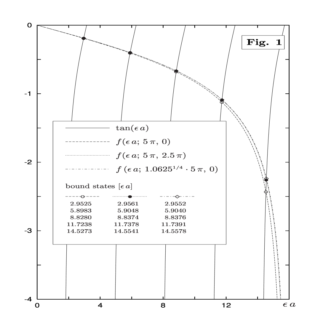
Figure 1: Graphical solutions of equation (17). The circle, bullet and diamond symbols respectively represent the vanishing angular momentum bound state solutions of the radial Schrödinger equation for a complex $(\,i\,V_{\mbox{\tiny$1$}}\,)$, quaternionic $(\,i\,V_{\mbox{\tiny$1$}}+j\,\,V_{\mbox{\tiny$2$}}+k\,V_{\mbox{\tiny$3$}}\,)$, and trial-complex $\left(\,i\,\sqrt{V_{\mbox{\tiny$1$}}^{{}^{\mbox{\tiny$2$}}}+V_{\mbox{\tiny$2$}}^{{}^{\mbox{\tiny$2$}}}+V_{\mbox{\tiny$3$}}^{{}^{\mbox{\tiny$2$}}}}\,\right)$ square-well potential. For the convenience of the reader we also list the numerical values of the bound energies. The plots refer to the following potentials: $a\sqrt{2m\,V_{\mbox{\tiny$1$}}/\hbar^{\mbox{\tiny$2$}}}=5\,\pi$ and $a\sqrt{2m\,\sqrt{V_{\mbox{\tiny$2$}}^{\mbox{\tiny$2$}}+V_{\mbox{\tiny$3$}}^{\mbox{\tiny$2$}}}/\hbar^{\mbox{\tiny$2$}}}=2.5\,\pi$.

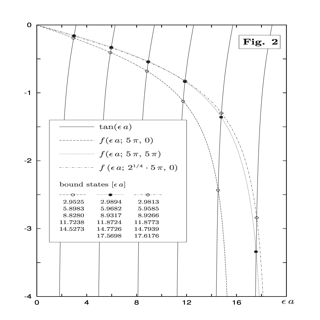
Figure 2: Graphical solutions of equation (17). The circle, bullet and diamond symbols respectively represent the vanishing angular momentum bound state solutions of the radial Schrödinger equation for a complex $(\,i\,V_{\mbox{\tiny$1$}}\,)$, quaternionic $(\,i\,V_{\mbox{\tiny$1$}}+j\,\,V_{\mbox{\tiny$2$}}+k\,V_{\mbox{\tiny$3$}}\,)$, and trial-complex $\left(\,i\,\sqrt{V_{\mbox{\tiny$1$}}^{{}^{\mbox{\tiny$2$}}}+V_{\mbox{\tiny$2$}}^{{}^{\mbox{\tiny$2$}}}+V_{\mbox{\tiny$3$}}^{{}^{\mbox{\tiny$2$}}}}\,\right)$ square-well potential. For the convenience of the reader we also list the numerical values of the bound energies. The plots refer to the following potentials: $a\sqrt{2m\,V_{\mbox{\tiny$1$}}/\hbar^{\mbox{\tiny$2$}}}=5\,\pi$ and $a\sqrt{2m\,\sqrt{V_{\mbox{\tiny$2$}}^{\mbox{\tiny$2$}}+V_{\mbox{\tiny$3$}}^{\mbox{\tiny$2$}}}/\hbar^{\mbox{\tiny$2$}}}=5\,\pi$.

One may ask wheter this is still true for energy values below $\sqrt{V_{\mbox{\tiny$2$}}^{{}^{\mbox{\tiny$2$}}}+V_{\mbox{\tiny$3$}}^{{}^{\mbox{\tiny$2$}}}}$. For $E<\sqrt{V_{\mbox{\tiny$2$}}^{{}^{\mbox{\tiny$2$}}}+V_{\mbox{\tiny$3$}}^{{}^{\mbox{\tiny$2$}}}}$, it can be immediately seen that $\nu_{\pm}$ and $zw$ are complex and this seems to be too restrictive. Consequently, no bound states should be expected for $E<\sqrt{V_{\mbox{\tiny$2$}}^{{}^{\mbox{\tiny$2$}}}+V_{\mbox{\tiny$3$}}^{{}^{\mbox{\tiny$2$}}}}$. Nevertheless, by simple algebraic manipulations (see appendix B for the explicit calculations), it can be shown that Eq.(17) still represents a real equation and bound states could exist below the pure quaternionic potential. Graphical solutions of equation (17) give the energies of the bound states of a particle in a quaternionic spherically symmetric potential trap, see Fig.1 and Fig.2. It is also instructive to compare the quaternionic bound states with the bound states of the trial-complex potential $\sqrt{V_{\mbox{\tiny$1$}}^{{}^{\mbox{\tiny$2$}}}+V_{\mbox{\tiny$2$}}^{{}^{\mbox{\tiny$2$}}}+V_{\mbox{\tiny$3$}}^{{}^{\mbox{\tiny$2$}}}}$.

IV CONCLUSIONS

This work was intended as an attempt at motivating the study of quaternionic formulations of quantum mechanics and at looking for deviations from the standard complex theory. The analysis presented in this paper represents a preliminary discussion on quaternionic bound states and touched only a few aspects of the theory. In particular, no attempt has been made here to develop a quaternionic perturbation theory or to study the behavior of confined quaternionic wave packets. These topics exceed the scope of this paper but surely represent important points to be investigated in view of a complete understanding of how and where quaternionic potentials could be seen and if  they really exist in nature.

Appendix A

To calculate the radial solution in region II, we have to solve a second order differential equation with quaternionic constant coefficients,

$$\left\{\,i\,\frac{\hbar^{\mbox{\tiny$2$}}}{2m}\,\frac{\mbox{d}^{\mbox{\tiny$2$}}}{\mbox{d}r^{\mbox{\tiny$2$}}}-i\,V_{\mbox{\tiny$1$}}-j\,V_{\mbox{\tiny$2$}}-k\,V_{\mbox{\tiny$3$}}\,\right\}\,U_{\mbox{\tiny II},\mbox{\tiny$\mathbb{H}$}}(r)=-\,U_{\mbox{\tiny II},\mbox{\tiny$\mathbb{H}$}}(r)\,i\,E~{}.$$ (19)

We refer the reader to [4, 20] for a detailed analysis of quaternionic differential operators. In this appendix, we will touch only a few aspect of the theory, by restricting our attention to differential operators with quaternionic constant coefficients. A (right-complex linear) solution of Eq.(19) can be written in terms of (left-acting) quaternionic ($q$) and complex ($\nu$) coefficients, i.e.

$$q\,\exp[\nu\,r]\,\,.$$

To determine this coefficients, let us apply to Eq.(19) the anti-Hermitian operator

$$i\,\frac{\hbar^{\mbox{\tiny$2$}}}{2m}\,\frac{\mbox{d}^{\mbox{\tiny$2$}}}{\mbox{d}r^{\mbox{\tiny$2$}}}-i\,V_{\mbox{\tiny$1$}}-j\,V_{\mbox{\tiny$2$}}-k\,V_{\mbox{\tiny$3$}}\,\,.$$

In this way we obtain

$$\left\{-\left(\frac{\hbar^{\mbox{\tiny$2$}}}{2m}\right)^{\mbox{\tiny$2$}}\,\frac{\mbox{d}^{\mbox{\tiny$4$}}}{\mbox{d}r^{\mbox{\tiny$4$}}}\,+\,2\,\frac{\hbar^{\mbox{\tiny$2$}}}{2m}\,V_{\mbox{\tiny$1$}}\,\frac{\mbox{d}^{\mbox{\tiny$2$}}}{\mbox{d}r^{\mbox{\tiny$2$}}}\,-\,\left(V^{{}^{\mbox{\tiny$2$}}}_{\mbox{\tiny$1$}}+V^{{}^{\mbox{\tiny$2$}}}_{\mbox{\tiny$2$}}+V^{{}^{\mbox{\tiny$2$}}}_{\mbox{\tiny$3$}}\right)\right\}\,U_{\mbox{\tiny II},\mbox{\tiny$\mathbb{H}$}}(r)=-\,E^{{}^{\mbox{\tiny$2$}}}\,U_{\mbox{\tiny II},\mbox{\tiny$\mathbb{H}$}}(r)~{},$$ (20)

which represents a real differential equation. Consequently, the quaternionic factor $q$ can be factorized and the complex coefficient $\nu$ is calculated once solved the following algebraic equation

$$\left(\frac{\hbar^{\mbox{\tiny$2$}}}{2m}\right)^{\mbox{\tiny$2$}}\,\nu^{\mbox{\tiny$4$}}-2\,\frac{\hbar^{\mbox{\tiny$2$}}}{2m}\,V_{\mbox{\tiny$1$}}\,\nu^{\mbox{\tiny$2$}}+V^{{}^{\mbox{\tiny$2$}}}_{\mbox{\tiny$1$}}+V^{{}^{\mbox{\tiny$2$}}}_{\mbox{\tiny$2$}}+V^{{}^{\mbox{\tiny$2$}}}_{\mbox{\tiny$3$}}-E^{{}^{\mbox{\tiny$2$}}}=0~{}.$$ (21)

The solutions for the complex coefficients $\nu$ are given by

$$\nu_{\mbox{\tiny$1$},\mbox{\tiny$2$}}=\pm\,\nu_{\mbox{\tiny$-$}}\,\,\,\,\,\mbox{and}\,\,\,\,\,\nu_{\mbox{\tiny$3$},\mbox{\tiny$4$}}=\pm\,\nu_{\mbox{\tiny$+$}}\,\,,\,\,\,\,\,\,\,\mbox{where}\,\,\,\mbox{$\nu_{\mbox{\tiny$\pm$}}=\sqrt{\frac{2m}{\hbar^{\mbox{\tiny$2$}}}\,\left(V_{\mbox{\tiny$1$}}\pm\sqrt{E^{{}^{\mbox{\tiny$2$}}}-V_{\mbox{\tiny$2$}}{{}^{{}^{\mbox{\tiny$2$}}}}-V_{\mbox{\tiny$3$}}^{{}^{\mbox{\tiny$2$}}}}\,\right)}$}\,\,.$$ (22)

Coming back to Eq.(19), for $E\neq\sqrt{V_{\mbox{\tiny$2$}}{{}^{{}^{\mbox{\tiny$2$}}}}+V_{\mbox{\tiny$3$}}^{{}^{\mbox{\tiny$2$}}}}$ and $E\neq\sqrt{V_{\mbox{\tiny$1$}}{{}^{{}^{\mbox{\tiny$2$}}}}+V_{\mbox{\tiny$2$}}{{}^{{}^{\mbox{\tiny$2$}}}}+V_{\mbox{\tiny$3$}}^{{}^{\mbox{\tiny$2$}}}}$ we then find four (right-complex) linear independent solutions[4], i.e.

$$q_{\mbox{\tiny$-$}}\,\exp[-\nu_{\mbox{\tiny$-$}}\,r]\,\,,\,\,\,\,\,q_{\mbox{\tiny$-$}}\,\exp[\nu_{\mbox{\tiny$-$}}\,r]\,\,,\,\,\,\,\,q_{\mbox{\tiny$+$}}\,\exp[-\nu_{\mbox{\tiny$+$}}\,r]\,\,\,\,\,\mbox{and}\,\,\,\,\,q_{\mbox{\tiny$+$}}\,\exp[\nu_{\mbox{\tiny$+$}}\,r]\,\,\,.$$

To find the quaternionic factor, $q_{\mbox{\tiny$-$}}$ (associated to $\exp[\pm\,\nu_{\mbox{\tiny$-$}}r]$) we set $q_{\mbox{\tiny$-$}}=1+j\,w$ ($w\in\mathbb{C}$). This choice is possible due to the right-complex linearity of the quaternionic differential equation (19). It follows immediately that

$$i\,(1+j\,w)\,\left(V_{\mbox{\tiny$1$}}-\sqrt{E^{{}^{\mbox{\tiny$2$}}}-V_{\mbox{\tiny$2$}}^{{}^{\mbox{\tiny$2$}}}-V_{\mbox{\tiny$3$}}^{{}^{\mbox{\tiny$2$}}}}\,\right)-\left(i\,V_{\mbox{\tiny$1$}}+j\,V_{\mbox{\tiny$2$}}+k\,V_{\mbox{\tiny$3$}}\right)(1+j\,w)=-\,(1+j\,w)\,i\,E~{}.$$

It is easy to check that the previous equation implies

$$i\left(E-\sqrt{E^{{}^{\mbox{\tiny$2$}}}-V_{\mbox{\tiny$2$}}^{{}^{\mbox{\tiny$2$}}}-V_{\mbox{\tiny$3$}}^{{}^{\mbox{\tiny$2$}}}}\,\right)+(V_{\mbox{\tiny$2$}}+i\,V_{\mbox{\tiny$3$}})\,w=0\,\,,$$

$$i\left(E+\sqrt{E^{{}^{\mbox{\tiny$2$}}}-V_{\mbox{\tiny$2$}}^{{}^{\mbox{\tiny$2$}}}-V_{\mbox{\tiny$3$}}^{{}^{\mbox{\tiny$2$}}}}\,\right)\,w-(V_{\mbox{\tiny$2$}}-i\,V_{\mbox{\tiny$3$}})=0\,\,.$$ (23)

Finally,

$$w=-\,i\,\frac{E\,-\,\sqrt{E^{{}^{\mbox{\tiny$2$}}}-V_{\mbox{\tiny$2$}}^{{}^{\mbox{\tiny$2$}}}-V_{\mbox{\tiny$3$}}^{{}^{\mbox{\tiny$2$}}}}}{V_{\mbox{\tiny$2$}}\,+\,i\,V_{\mbox{\tiny$3$}}}=-\,i\,\frac{V_{\mbox{\tiny$2$}}\,-\,i\,V_{\mbox{\tiny$3$}}}{E\,+\,\sqrt{E^{{}^{\mbox{\tiny$2$}}}-V_{\mbox{\tiny$2$}}^{{}^{\mbox{\tiny$2$}}}-V_{\mbox{\tiny$3$}}^{{}^{\mbox{\tiny$2$}}}}}~{}.$$ (24)

To find the quaternionic factor, $q_{\mbox{\tiny$+$}}$ (associated to $\exp[\pm\,\nu_{\mbox{\tiny$+$}}r]$) we choose $q_{\mbox{\tiny$+$}}=z+j$ ($z\in\mathbb{C}$). A calculation similar to previous one gives

$$z=\,i\,\frac{E\,-\,\sqrt{E^{{}^{\mbox{\tiny$2$}}}-V_{\mbox{\tiny$2$}}^{{}^{\mbox{\tiny$2$}}}-V_{\mbox{\tiny$3$}}^{{}^{\mbox{\tiny$2$}}}}}{V_{\mbox{\tiny$2$}}\,-\,i\,V_{\mbox{\tiny$3$}}}=\,i\,\frac{V_{\mbox{\tiny$2$}}\,+\,i\,V_{\mbox{\tiny$3$}}}{E\,+\,\sqrt{E^{{}^{\mbox{\tiny$2$}}}-V_{\mbox{\tiny$2$}}^{{}^{\mbox{\tiny$2$}}}-V_{\mbox{\tiny$3$}}^{{}^{\mbox{\tiny$2$}}}}}~{}.$$ (25)

Appendix B

In this appendix, we are interested to prove that Eq.(17) for $E<\sqrt{V_{\mbox{\tiny$2$}}^{{}^{\mbox{\tiny$2$}}}+V_{\mbox{\tiny$3$}}^{{}^{\mbox{\tiny$2$}}}}$ still represents a real equation. Before to proceed with the proof, let us observe that

$$z\,w=\exp\left[-2\,i\,\arctan\frac{\sqrt{V_{\mbox{\tiny$2$}}^{{}^{\mbox{\tiny$2$}}}+V_{\mbox{\tiny$3$}}^{{}^{\mbox{\tiny$2$}}}-E^{{}^{\mbox{\tiny$2$}}}}}{E}\right]$$

and

$$\nu_{\mbox{\tiny$\pm$}}=\mbox{$\sqrt{\frac{2m}{\hbar^{\mbox{\tiny$2$}}}}\left[\frac{1}{\sqrt{2}}\,\sqrt{V_{\mbox{\tiny$1$}}+\sqrt{V_{\mbox{\tiny$1$}}^{{}^{\mbox{\tiny$2$}}}+V_{\mbox{\tiny$2$}}^{{}^{\mbox{\tiny$2$}}}+V_{\mbox{\tiny$3$}}^{{}^{\mbox{\tiny$2$}}}-E^{{}^{\mbox{\tiny$2$}}}}}\pm i\frac{1}{\sqrt{2}}\,\sqrt{\sqrt{V_{\mbox{\tiny$1$}}^{{}^{\mbox{\tiny$2$}}}+V_{\mbox{\tiny$2$}}^{{}^{\mbox{\tiny$2$}}}+V_{\mbox{\tiny$3$}}^{{}^{\mbox{\tiny$2$}}}-E^{{}^{\mbox{\tiny$2$}}}}-V_{\mbox{\tiny$1$}}}\right]$}\,\,.$$

It is natural to rewrite Eq.(17) as follows

$$\tan(\epsilon\,a) = -\,\epsilon\,\,\frac{\left(\,\nu_{\mbox{\tiny$+$}}-z\,w\,\nu_{\mbox{\tiny$-$}}\,\right)\,\tanh(\epsilon\,a)+\left(\,1-z\,w\,\right)\,\epsilon}{\nu_{\mbox{\tiny$-$}}\,\nu_{\mbox{\tiny$+$}}\,\left(\,1-z\,w\,\right)\,\tanh(\epsilon\,a)+\left(\,\nu_{\mbox{\tiny$-$}}-z\,w\,\nu_{\mbox{\tiny$+$}}\,\right)\,\epsilon}\,$$ (26)

$$= -\,\epsilon\,\,\frac{\mbox{\sc Num}}{\mbox{\sc Den}}=-\,\epsilon\,\,\frac{\mbox{\sc Num}\,\,\overline{\mbox{\sc Den}}}{\left|\mbox{\sc Den}\right|^{\mbox{\tiny$2$}}}\,\,.$$

The important point to note here is that

$$\nu_{\mbox{\tiny$+$}}=\overline{\nu_{\mbox{\tiny$-$}}}\,\,\,\,\,\,\,\,\mbox{and}\,\,\,\,\,\,\,\,|z\,w|=1\,\,.$$

We can now proceed with the proof,

$$\mbox{\sc Num}\,\,\overline{\mbox{\sc Den}} = \left[\,\left(\,\nu_{\mbox{\tiny$+$}}-z\,w\,\nu_{\mbox{\tiny$-$}}\,\right)\,\tanh(\epsilon\,a)+\left(\,1-z\,w\,\right)\,\epsilon\,\right]\left[\,|\nu_{\mbox{\tiny$-$}}|^{\mbox{\tiny$2$}}\,\left(\,1-\overline{z\,w}\,\right)\,\tanh(\epsilon\,a)+\left(\,\nu_{\mbox{\tiny$+$}}-\overline{z\,w}\,\nu_{\mbox{\tiny$-$}}\,\right)\,\epsilon\,\right]$$ (27)

$$= \left(\,\nu_{\mbox{\tiny$-$}}-z\,w\,\nu_{\mbox{\tiny$-$}}+\overline{\nu_{\mbox{\tiny$-$}}}-\overline{z\,w}\,\overline{\nu_{\mbox{\tiny$-$}}}\,\right)\,|\nu_{\mbox{\tiny$-$}}|^{\mbox{\tiny$2$}}\,\tanh^{\mbox{\tiny$2$}}(\epsilon\,a)\,+$$

$$\left[\,\nu_{\mbox{\tiny$-$}}^{\,\mbox{\tiny$2$}}+\overline{\nu_{\mbox{\tiny$-$}}}^{\,\mbox{\tiny$2$}}-(z\,w+\overline{z\,w})\,|\nu_{\mbox{\tiny$-$}}|^{\mbox{\tiny$2$}}+(1-z\,w)\,(1-\overline{z\,w})\,|\nu_{\mbox{\tiny$-$}}|^{\mbox{\tiny$2$}}\,\right]\,\epsilon\,\tanh(\epsilon\,a)\,+$$

$$\left(\,\nu_{\mbox{\tiny$-$}}-\overline{z\,w}\,\nu_{\mbox{\tiny$-$}}+\overline{\nu_{\mbox{\tiny$-$}}}-z\,w\,\overline{\nu_{\mbox{\tiny$-$}}}\,\right)\,\epsilon^{\mbox{\tiny$2$}}$$

$$\in \mathbb{R}\,\,.$$