On positive functions with positive Fourier transforms

Abstract

Using the basis of Hermite-Fourier functions (i.e. the quantum oscillator eigenstates) and the Sturm theorem, we derive the practical constraints for a function and its Fourier transform to be both positive. We propose a constructive method based on the algebra of Hermite polynomials. Applications are extended to the 2-dimensional case (i.e. Fourier-Bessel transforms and the algebra of Laguerre polynomials) and to adding constraints on derivatives, such as monotonicity or convexity.

I Introduction

Positivity conditions for a Fourier transform appear in various domains of Physics. Frequent questions are,

• What are the constraints for a real function $\psi(r)$ ensuring that its Fourier transform,

  $$\varphi(s)=\frac{1}{\sqrt{2\pi}}\,\int_{-\infty}^{+\infty}dr\ e^{isr}\,\psi(r)\,,$$ (1)

  be real and positive?

• Conversely, what are the properties of $\varphi$ if $\psi$ is positive?

• Finally, what are the constraints on Fourier partners such that both $\psi$ and $\varphi$ be positive?

Physicists often need to work with concrete constructions. The practical construction of a basis of functions satisfying the abovementionned positivity properties remains, up to our knowledge, an open problem. Such questions are quite relevant in Physics. As practical examples, let us quote two well-known cases. A Fourier transform relates [1] two quantities, namely the cross section and the profile of a nucleus, which ought to be both positive. In Particle Physics, a 2-d Fourier-Bessel transform relates the color dipole distribution in transverse position space (derived from Quantum Chromodynamics) and the transverse momentum distribution of gluons probed during a deep-inelastic collision [2]. In short, such questions occur also in probability calculus, for the relation between probability distributions and characteristic functions [3], in crystallography and more generally in condensed matter physics, e.g. for the interpretation of patterns, etc….

The problem is simplified if related to another one, that concerning the functions which are invariant [4] up to a phase factor by Fourier transforms. Indeed, the most familiar examples of positive self-dual functions or distributions, thus trivially verifying the double positivity condition, which are at most scaled under Fourier transformation (FT), are the Gaussian and the Dirac comb. Many special cases can be found, where positivity is conserved, such as, for instance, the continuous family of functions $\exp(-r^{\nu}),$ where $0<\nu\leq 2.$ Various sufficient conditions for positivity can be found in the literature, such as the convexity of $\psi$ [7] but, up to our knowledge, no general constructive method has been presented.

The present note attempts to give general positivity criteria, in a constructive way, by taking advantage of a representation under which the FT is essentially “transparent”. Our method combines the advantages of self-duality properties with those allowed by an algebra of polynomials, where positivity means absence of real roots, hence explicit manipulations of polynomial coefficients. For this sake, in the 1-d case, we select a basis made of convenient eigenstates of the FT, the Hermite-Fourier functions, i.e. the harmonic oscillator eigenstates. The method extends to the 2-d case, or Fourier-Bessel transform, by replacing Hermite by Laguerre polynomials.

There are general mathematical theorems about the characterization of Fourier transforms of positive functions [8]. Let us quote in the first place the Bochner theorem and its generalizations [9] which state that the Fourier transform of a positive function is positive-definite. But positive definiteness in the sense of such theorems does not imply plain positivity. Hence our problem actually could be rephrased [10] as “build positive-definite functions that are positive”.

Our formalism is the subject of Section II. Numerical, illustrative examples will be given in Section III. Then Section IV describes the extension of our algorithms to the 2-d problem. Hermite polynomials will be replaced by Laguerre ones, but the algebra remains essentially the same. A brief discussion, conclusion and outlook make Section V.

II Basic formalism

Consider the harmonic oscillator Hamiltonian, $\frac{1}{2}(p^{2}+r^{2}),$ and its eigenwavefunctions,

$$u_{n}(r)=\pi^{-\frac{1}{4}}\,e^{-\frac{1}{2}r^{2}}H_{n}(r).$$ (2)

Here, we set $H_{n}$ to be a square normalized Hermite polynomial, with a positive coefficient for its highest power term. For the sake of clarity, we list the first polynomials as, $H_{0}=1,\,H_{1}=\sqrt{2}\ r,\,H_{2}=(2r^{2}-1)/\sqrt{2},\,H_{3}=(2r^{3}-3r)/\sqrt{3}\,$ and their recursion relation

$$a_{n+1}H_{n+1}=2\,r\,a_{n}H_{n}-2\,n\,a_{n-1}H_{n-1}\ ,$$ (3)

where $a_{n}=\sqrt{2^{n}n!}\ .$ It is known that the FT of such states brings only a phase,

$$\frac{1}{\sqrt{2\pi}}\,\int_{-\infty}^{\infty}dr\ e^{isr}\,u_{n}(r)=i^{n}\ u_{n}(s)\,,$$ (4)

and thus such states give generalized self-dual functions with phase $i^{n}.$ If one expands $\psi$ in the oscillator basis, $\psi(r)=\sum_{n=0}^{N}\psi_{n}\,u_{n}(r),$ with a truncation at some degree $N,$ then all odd components $\psi_{2p+1}$ must vanish if $\varphi$ must be real, and the even rest splits, under FT, into an invariant part and a part with its sign reversed, namely

$$\varphi(s)=\pi^{-\frac{1}{4}}\,e^{-\frac{1}{2}s^{2}}\ [P_{+}(s)-P_{-}(s)],\ \ P_{+}(s)=\sum_{p=0}^{[N/4]}\psi_{4p}\,H_{4p}(s),\ \ P_{-}(s)=\sum_{p=0}^{[(N-2)/4]}\psi_{4p+2}\,H_{4p+2}(s)\,,$$ (5)

where the usual symbols $[N/4]$ and $[(N-2)/4]$ mean, respectively, the entire parts of $N/4$ and $(N-2)/4.$

Notice that, when all components $\psi_{n}$ vanish except $\psi_{0},$ then both $\psi$ and $\varphi$ are positive, because $H_{0}=1.$ Hence, one may, starting from this special point in the functional space of functions, investigate those domains of parameters $\psi_{n}$ where the polynomials ${\cal P}=P_{+}+P_{-}$ and ${\cal Q}=P_{+}-P_{-}$ have no real root. Notice that only even powers of $r$ and $s$ are involved. It will therefore be convenient to use auxiliary variables such as $\rho=r^{2}$ and $\sigma=s^{2},$ and the domain of interest for the parameters $\psi_{n}$ will correspond to the absence of real positive roots for both $\rho$ and $\sigma.$

The second ingredient of our approach is the well-known Sturm theorem [11] which gives the efficient way to characterize and localize the real roots of any given polynomial. The Sturm criterion can be expressed as follows:

“ Given a polynomial ${\cal P}(x),$ its Sturm sequence ${\cal S}(x)\equiv\left\{{\cal S}_{1},{\cal S}_{2},...\ {\cal S}_{m},...{\cal S}_{j\leq N}\right\}$ is the set of polynomials

$${\cal S}_{1}={\cal P},\ {\cal S}_{2}=d{\cal P}/dx,\ ...\ {\cal S}_{m}=-{\cal S}_{m-2}+\left[\frac{{\cal S}_{m-2}}{{\cal S}_{m-1}}\right]\,{\cal S}_{m-1}\ ...\ ,$$ (6)

where $\bf[\frac{\ }{\ }]$ designates the polynomial quotient. To know the number of roots between $x=a$ and $x=b,$ count the number ${\cal N}(a)$ of sign changes in ${\cal S}(a)$ and, similarly, count ${\cal N}(b).$ Then the number of roots is $\left|{\cal N}(b)-{\cal N}(a)\right|.$ ”

The domain borders where the root number, $\left|{\cal N}(+\infty)-{\cal N}(0)\right|,$ changes have to do with cancellations of the resultant $\cal R$ between ${\cal P}$ and $d{\cal P}/dx.$ The cancellation of ${\cal R}$ corresponds to collisions between conjugate complex roots becoming real roots and conversely. Because of the demanded positivity of $\rho$ and $\sigma,$ the borders have also to do with sign changes of ${\cal P}(0)$ and ${\cal Q}(0),$ meaning real roots $\rho$ and $\sigma$ going through $0.$ All such technicalities are taken care of by the Sturm criterion, which furthermore allows the labeling of each domain by its precise number of real roots.

This will be implemented here in an explicit way, analytically as much as possible, then numerically and graphically, for a few cases of a general illustrative value. For this, we will plot the shapes of domains labeled by the values of the Sturm criterion. Hence the combination of the self-dual properties of the quantum oscillator basis and of the Sturm theorem allows a constructive method for a systematic investigation of positivity conditions for a 1-d Fourier transform. This basis has the potential to represent any function in the Hilbert space ${\cal L}^{2}$, but the present study concerns a finite set of components. An extension to infinite series of components may deserve other tools.

III Positivity domains

In this Section we will apply our method to the case of a basis formed with 3 or 4 Hermite-Fourier functions. We consider: A the basis ${\psi_{0},\psi_{4},\psi_{8}},$ then B the basis ${\psi_{0},\psi_{4},\psi_{8},\psi_{12}},$ which both lie in the subspace with eigenvalue $1$, and C the basis ${\psi_{0},\psi_{2},\psi_{4}}$ where $\psi_{2}$ is in the subspace with eigenvalue $-1,$ furthermore, D the influence of an additional constraint motivated by Physics, that of monotony for $\varphi,$ and finally E a comparison with the convexity constraint for $\psi.$ Many other illustrations are possible, but these, A-E, demonstrate the flexibility of our approach.

A Mixture of three polynomials in the subspace with eigenvalue 1

Here we assume that $\psi$ has only components $\psi_{0},$ $\psi_{4}$ and $\psi_{8},$ hence ${\cal P}$ reduces to $P_{+}$ in (5) and we can study

$${\cal P}=\psi_{0}+\frac{\psi_{4}\,}{2\,\sqrt{6}}\,(4\rho^{2}-12\rho+3)+\frac{\psi_{8}\,}{24\,\sqrt{70}}\,(16\rho^{4}-224\rho^{3}+840\rho^{2}-840\rho+105\,),$$ (7)

where $\rho=r^{2}.$ One maintains $\psi_{8}>0$ and one reads $P_{+}(0)=\psi_{0}+3\psi_{4}/(2\,\sqrt{6})+105\psi_{8}/(24\,\sqrt{70}).$ The resultant ${\cal R}$ between $P$ and $dP/d\rho$ is,

$${\cal R}\propto 2100\,\psi_{0}\,\psi_{4}^{4}-1050\,\sqrt{6}\,\psi_{4}^{5}-240\,\sqrt{70}\,\psi_{0}^{2}\,\psi_{4}^{2}\,\psi_{8}+400\,\sqrt{105}\,\psi_{0}\,\psi_{4}^{3}\,\psi_{8}-165\,\sqrt{70}\,\psi_{4}^{4}\,\psi_{8}+$$ (8)

$$480\,\psi_{0}^{3}\,\psi_{8}^{2}+4560\,\sqrt{6}\,\psi_{0}^{2}\,\psi_{4}\,\psi_{8}^{2}-13320\,\psi_{0}\,\psi_{4}^{2}\,\psi_{8}^{2}-1600\,\sqrt{6}\,\psi_{4}^{3}\,\psi_{8}^{2}-792\,\sqrt{70}\,\psi_{0}^{2}\,\psi_{8}^{3}+$$ (9)

$$1728\,\sqrt{105}\,\psi_{0}\,\psi_{4}\,\psi_{8}^{3}-612\,\sqrt{70}\,\psi_{4}^{2}\,\psi_{8}^{3}-10080\,\psi_{0}\,\psi_{8}^{4}-2520\,\sqrt{6}\,\psi_{4}\,\psi_{8}^{4}+1260\,\sqrt{70}\,\psi_{8}^{5}\,.$$ (10)

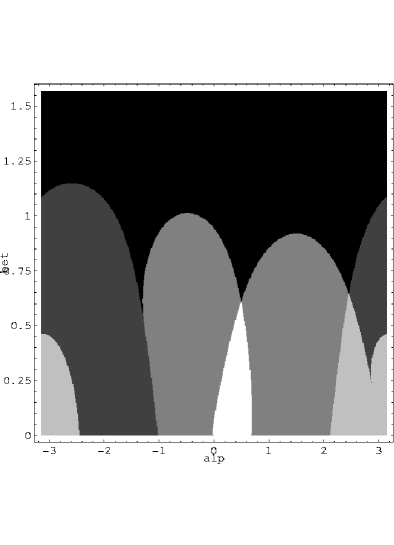
FIG. 1.: Mixture of $H_{0},$ $H_{4}$ and $H_{8}.$ White, no real positive $\rho$ root; black, 4 roots; darkening grays, increasing root number.

It is convenient to take advantage of the free scaling of ${\cal P}$ and normalize the polynomial so that its coefficients lie on a half sphere of unit radius,

$$\psi_{0}=\cos\alpha\,\cos\beta,\ \ \psi_{4}=\sin\alpha\,\cos\beta,\ \ \psi_{8}=\sin\beta,\ \ \ \ -\pi<\alpha\leq\pi,\ \ 0<\beta\leq\pi/2\,.$$ (11)

We thus show in Figure 1 the domains where the number of roots increases from 0 to 4. The no root domain is the white triangle above $\alpha=\beta=0$ and slightly right from this point. In this domain, $\psi\ (\equiv\varphi)$ is self-Fourier and positive.

B Mixture of four polynomials in the subspace with eigenvalue 1

Now we add to $\psi$ a component $\psi_{1\!2},$ hence

$${\cal P} = \psi_{0}+\frac{\psi_{4}}{2\,\sqrt{6}}\,(4\rho^{2}-12\rho+3)+\frac{\psi_{8}\,}{24\,\sqrt{70}}\,(16\rho^{4}-224\rho^{3}+840\rho^{2}-840\rho+105\,)+$$ (13)

$$\frac{\psi_{1\!2}\,}{1440\,\sqrt{231}}\,(64\rho^{6}-2112\rho^{5}+23760\rho^{4}-110880\rho^{3}+207900\rho^{2}-124740\rho+10395\,).$$

While borders corresponding to $P_{+}(0)=0$ obtain easily, the resultant ${\cal R}$ to be considered for other borders is unwieldy and is skipped here. Taking advantage of scaling we set,

$$\psi_{0}=\cos\alpha\,\cos\beta\,\cos\gamma,\ \ \psi_{4} = \sin\alpha\,\cos\beta\,\cos\gamma,\ \ \psi_{8}=\sin\beta\cos\gamma,\ \ \psi_{1\!2}=\sin\gamma,$$ (14)

$$-\frac{\pi}{2}<\alpha\leq\frac{\pi}{2} \ -\pi<\beta\leq\pi\,,\ \ \ 0<\gamma\leq\frac{\pi}{2}\,.$$ , (15)

This choice of spherical coordinates was designed to ensure the positivity of $\psi_{1\!2},$ obviously, but also a dominance of $\psi_{0}$ near $\alpha\!=\!\beta\!=\!\gamma\!=\!0.$ The dominance is clearly useful for the positivity of ${\cal P}.$ Then this $S_{3}$ sphere can be explored by various cuts according to fixed values of $\gamma.$ The results are shown in Figures 2-5, with $\gamma=\pi/10^{6},\,\pi/15,\,2\pi/15,\,\pi/6,\,\pi/5,\,7\pi/30,\,4\pi/15,\,3\pi/10\,,$ respectively. The color code for the number of roots is: 0 root, red; 1, yellow; 2, yellowish green; 3, bluish green; 4, blue; 5, dark purple; 6, pink (in the uncolored edition, the no root domain, if it exists, is that dark, small or tiny triangle slightly right of the map center). The red domain shrinks at first very slowly when $\gamma$ increases, then faster when $\gamma\simeq\pi/6.$ Beyond such an order of magnitude for $\gamma,$ there is no red domain and the map becomes invaded by bigger and bigger pink patches, representing the dominance of the $6$ positive, real roots of $H_{1\!2}.$

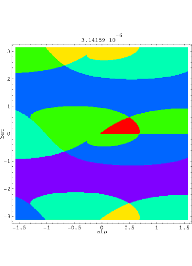
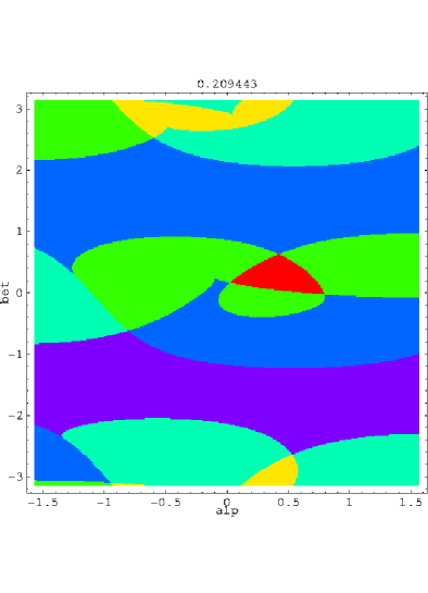
FIG. 2.: Mixture of $H_{0},$ $H_{4},$ $H_{8}$ and $H_{1\!2}.$ Root number maps. Color code: 0 root, red; 1, yellow; 2, yellowish green; 3, bluish green; 4, blue; 5, dark purple; 6, pink. Left: cut of the parameter sphere $S_{3}$ when $\gamma=\pi/10^{6}.$ Right: cut for $\gamma=\pi/15$ (uncolored edition: the $0$ root domain is the dark triangle-like domain near the center).

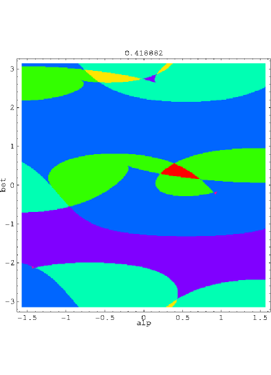
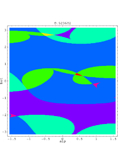
FIG. 3.: Left: Same as Fig. 2, with $\gamma=2\pi/15.$ Right: $\gamma=\pi/6.$ See how the no root triangle shrinks.

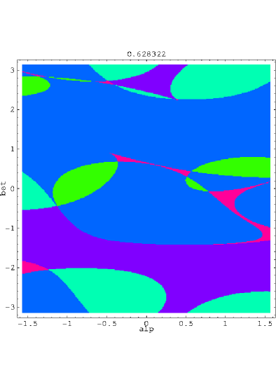
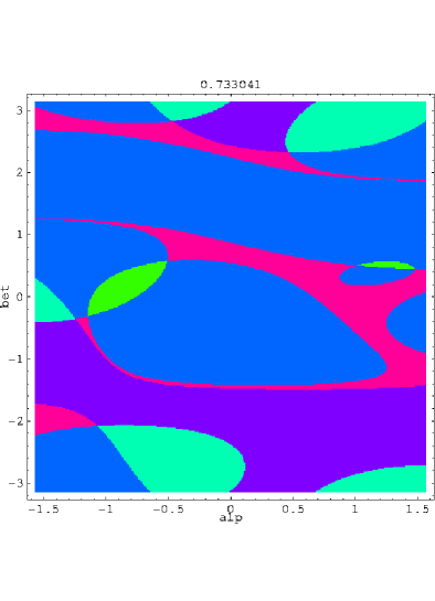
FIG. 4.: Left: $\gamma=\pi/5;$ Right: $\gamma=7\pi/30.$ Absence of no root domain.

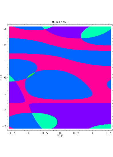
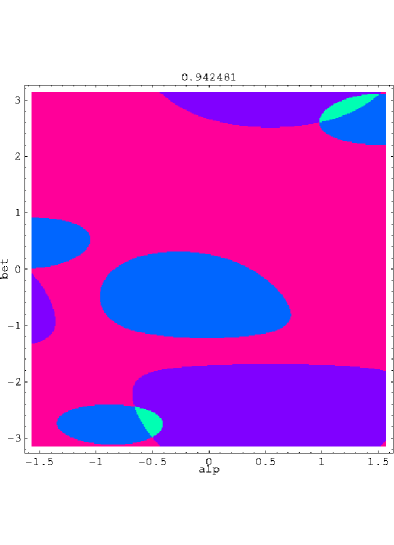
FIG. 5.: Left: $\gamma=4\pi/15;$ Right: $\gamma=3\pi/10.$ Progressive dominance of $H_{1\!2}$ with 6 $\rho$ roots.

C Two polynomials from subspace “$1$” mixed with one polynomial from subspace “$-1$”

If we consider a mixture of $H_{0},$ $H_{2}$ and $H_{4},$ the FT connects the two polynomials

$${\cal P}(\rho)=\psi_{0}+\psi_{2}\,\frac{2\rho-1}{\sqrt{2}}+\psi_{4}\,\frac{4\rho^{2}-12\rho+3}{2\,\sqrt{6}}\,,\ \ \ \ {\cal Q}(\sigma)=\psi_{0}-\psi_{2}\,\frac{2\sigma-1}{\sqrt{2}}+\psi_{4}\,\frac{4\sigma^{2}-12\sigma+3}{2\,\sqrt{6}}\,.$$ (16)

We study the positivity of each polynomial separately, then of both. Notice that the parametrization,

$$\psi_{0}=\cos\alpha\,\cos\beta,\ \ \psi_{2}=\sin\alpha\,\cos\beta,\ \ \psi_{4}=\sin\beta,\ \ \ \ -\pi<\alpha\leq\pi,\ \ 0<\beta\leq\pi/2\,,$$ (17)

reverses only the sign of $\psi_{2}$ if $\alpha$ becomes $-\alpha$. This parity operation is seen in Figure 6, the white domains of which correspond to the positivity of ${\cal P}$ and ${\cal Q},$ respectively. The domain of simultaneous positivity for both is the white intersection domain in the left part of Figure 7, with the expected symmetry.

It is actually easy here to analyze analytically the resultants of interest for ${\cal P}$ and ${\cal Q},$

$${\cal R}\propto\sqrt{6}\,\psi_{2}^{2}-4\,\psi_{0}\,\psi_{4}\ \ \mp\ 4\,\sqrt{2}\,\psi_{2}\,\psi_{4}+2\,\sqrt{6}\,\psi_{4}^{2},$$ (18)

together with signatures for the signs of roots, such as ${\cal P}(0),$ etc. This can be done also in the “spherical representation”. The white domains of Figs. 6, 7 are recovered.

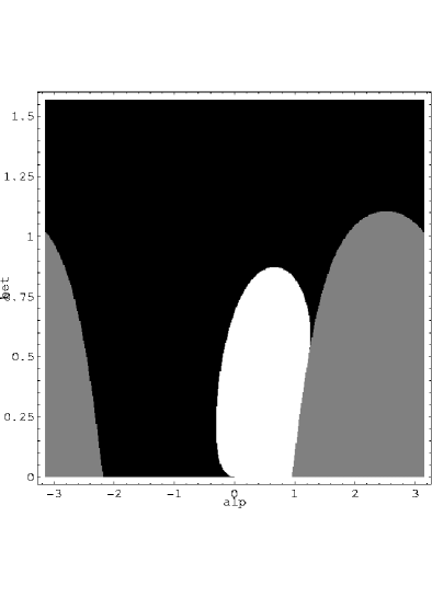
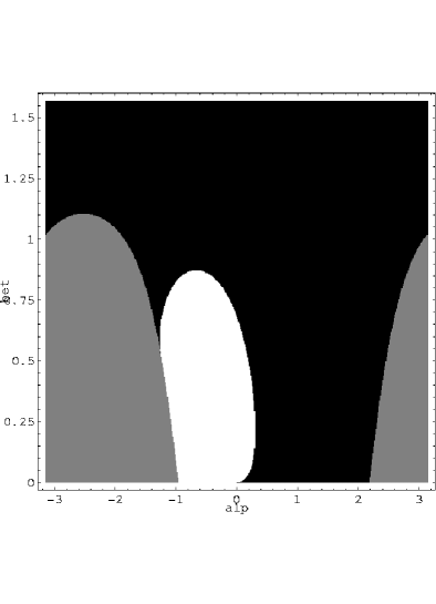
FIG. 6.: Mixture of $H_{0},$ $H_{2}$ and $H_{4}.$ White domain, 0 root. Grey, $1$ root; black, $2$ roots. Left: results for ${\cal P}$; Right: ${\cal Q}.$

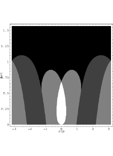
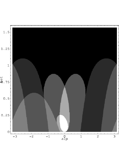
FIG. 7.: Positivity domains for the parity mixed case. Left: for both ${\cal P}$ and ${\cal Q}.$ Right: ${\cal P},$ ${\cal Q}$ and monotony of $\varphi.$

D Positivity with monotony

For some problems [2], it may be useful to request either $\psi$ and/or $\varphi$ to be monotonous functions in an interval such as $[0,\infty[.$ We illustrate this in the case of an $H_{0},H_{2},H_{4}$ mixture, with the additional constraint,

$$\frac{d\varphi}{d\sigma}\propto-12\,\cos\alpha\,\cos\beta+6\,\sqrt{2}\,\cos\beta\,\sin\alpha\,(2\sigma-5)-\sin\beta\,\sqrt{6}\,(4\sigma^{2}-28\sigma+27)<0\,.$$ (19)

The result appears in the right part of Fig. 7. The white domain, corresponding to such three simultaneous conditions of positivity and monotonicity, is a severe restriction of the white domain seen in the left part of Fig. 7.

E Positivity from convexity

A practical and sufficient, but not necessary condition for the positivity of $\varphi$ is the convexity of $\psi$ [7]. Indeed, $\varphi\sim\int_{0}^{\infty}dr\,[1-\cos(sr)]/s^{2}\,d^{2}\psi/dr^{2}>0.$ We illustrate this convexity condition for a mixture of $H_{0},H_{4},H_{8}.$ It is clear that the presence of $\exp\!\left(-r^{2}/2\right)$ in front of a finite order polynomial, with the even parity of $\psi$ and its derivability, are contradictory with “convexity everywhere”; a smooth, round maximum must occur at the origin. We thus study partial convexity conditions of the kind, “convexity between $r_{c}$ and $+\infty$”. A reasonable choice for the order of magnitude of $r_{c}$ is the position $r_{c}=1$ of the inflexion point of $\exp\!\left(-r^{2}/2\right).$ The second derivative $d^{2}\psi/dr^{2}$ belongs to the same algebra. We adjusted its Sturm criterion to various values of $r_{c}.$ Small domains only are found that ensure zero roots for $d^{2}\psi/dr^{2},$ because most mixtures of $H_{0},H_{4},H_{8}$ do oscillate. Figures 8 and 9 show, in white again, with the parametrization by Eqs. (11), the survivor domain obtained if $r_{c}=1,$ right part Fig. 8, then $r_{c}^{2}=2/3,$ left part Fig. 9, and $r_{c}^{2}=2/5,$ right part Fig. 9, respectively. The domain shrinks in a smooth way when $r_{c}^{2}$ decreases from $1$ to $0.4$ and disappears if $r_{c}^{2}<\sim 0.4.$ It does not increase much when $r_{c}\geq{\cal O}(1).$ The left part of Fig. 8, a zoom of the left part of Fig. 6, shows that such partial convexity domains are already included in the positivity domain of $\psi.$

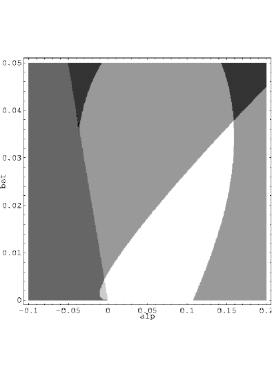
FIG. 8.: $H_{0},H_{4},H_{8}$ mixture. Left: zoom of the positivity domain. Right: convexity domain for $r>r_{c}=1.$

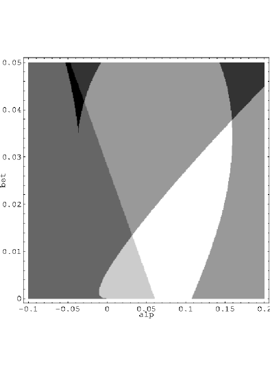
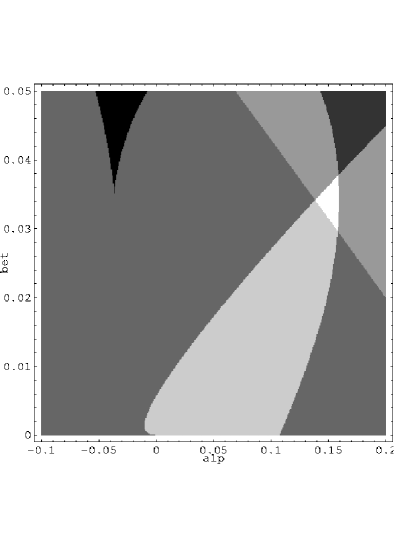
FIG. 9.: Same mixture as Fig. 8. Convexity domains. Left: $r_{c}^{2}=.67.$ Right: $r_{c}^{2}=.4.$

IV Positivity for the 2-dimensional Fourier transform

The Fourier-Bessel transform in which we are here interested reads,

$$\varphi(s)=\int_{0}^{\infty}(r\,dr)\,J_{0}(s\,r)\,\psi(r)\,.$$ (20)

For the 2-d radial space, a complete basis of states results from substituting $r^{2}$ for $r$ into Laguerre polynomials,

$$\int_{0}^{\infty}(r\,dr)\ 2\ e^{-r^{2}}\,L_{m}(r^{2})\,L_{n}(r^{2})=\delta_{mn}\,.$$ (21)

For the sake of clarity, we list here the first four such normalized, “2-d radial” states,

$$\{v_{0},\,v_{1},\,v_{2},\,v_{3}\}\ =\ \sqrt{2}\ e^{-\frac{1}{2}r^{2}}\,\left\{1,\,r^{2}-1,\,\frac{r^{4}-4r^{2}+2}{2},\,\frac{r^{6}-9r^{4}+18r^{2}-6}{6}\right\}\,.$$ (22)

One can verify that the states $v_{n}$ make eigenstates of the Fourier-Bessel transform,

$$\int_{0}^{\infty}(r\,dr)\,J_{0}(s\,r)\,v_{n}(r)=(-1)^{n}\,v_{n}(s)\,.$$ (23)

Positivity conditions can again be implemented with the Sturm criterion. For instance a mixture of $v_{0},v_{2},$ from that subspace with eigenvalue $1,$ and $v_{1},$ from that with eigenvalue $-1,$ defines the following two reciprocal partners,

$${\cal P}(\rho)=\psi_{0}+\psi_{1}\,(\rho-1)+\psi_{2}\,\frac{\rho^{2}-4\rho+2}{2}\,,\ \ \ \ {\cal Q}(\sigma)=\psi_{0}-\psi_{1}\,(\sigma-1)+\psi_{2}\,\frac{\sigma^{2}-4\sigma+2}{2}\,.$$ (24)

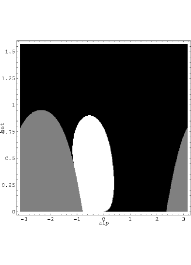
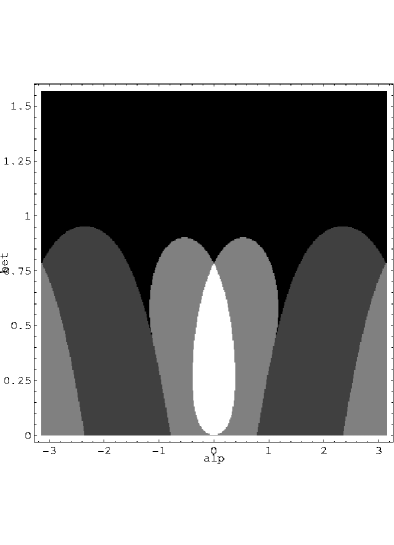
FIG. 10.: Positivity domains for the “radial 2-d”, parity mixed case. Left: $\varphi.$ Right: both $\psi$ and $\varphi.$

The left part of Figure 10 shows the positivity domain for $\varphi$ and its right part shows the joint positivity domain for $\psi$ and $\varphi.$ Similarities beween polynomials involved in the present “mixed parity” case and those of case C of the previous Section create topological similarities with Fig. 6 (right) and Fig. 7 (left) but numerical details do differ.

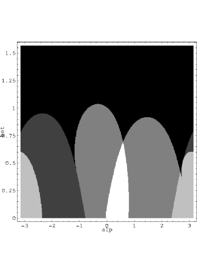
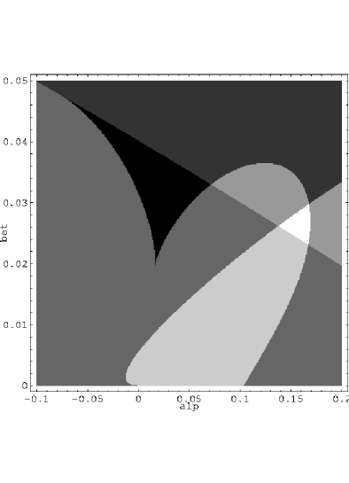
FIG. 11.: Left: Positivity domain for the “radial 2-d”, $v_{0},v_{2},v_{4}$ mixture. Right: third derivative negativity domain if $r_{t}^{2}=1.4.$

Interestingly enough, a sufficient condition [7] for the positivity of $\varphi$ in this 2-d situation is that the third derivative, $d^{3}\psi/dr^{3},$ be negative. But, as in the previous Section, case E, the presence of a truncated number of basis terms in our expansion may reduce this negativity condition for $d^{3}\psi/dr^{3}$ to a domain $r\geq r_{t}$ only. We show in Figure 11 the result for a mixture of $v_{0},$ $v_{2}$ and $v_{4}$ if $r_{t}^{2}=1.4,$ a demanding situation resulting into the tiny domain in the right part of Fig. 11. The domain belongs to the positivity domain seen in the left part of the same Figure.

V Discussion and Conclusion

To summarize our results, we have built a basis of functions verifying positivity together with their Fourier transform. The method is based upon algebras of Hermite polynomials (for 1-dimensional FT) or Laguerre polynomials in the variable $r^{2}$ (for 2-dimensional radial FT).

The Fourier transform has four eigenvalues $1,i,-1,-i,$ and thus four highly degenerate eigensubspaces. Two of such subspaces are compatible with real functions remaining real. To span each subspace, we used a basis made of Hermite-Fourier (or “Laguerre-Fourier”) states. The orders (in $r$) of the polynomials have to be multiples of $4$ if the eigenvalue is $1,$ and multiple of $4$ plus $2$ if the eigenvalue is $-1.$ At the cost of a truncation of such bases to a maximum order $N,$ the conditions for positivity, convexity, etc. thus reduce to simple manipulations of polynomial coefficients based on the Sturm theorem. In each truncation case, one can find suitable domains for the parameters which mix the various basis polynomials. Such domains have been illustrated by the figures shown by this paper.

FIG. 12.: Left: two examples of self Fourier states ($\varphi=\psi$). Right: mixed parity case ($\varphi\neq\psi$).

Some qualitative considerations may be drawn about the solutions we found in various examples. In the left part of Figure 12, we display two typical solutions with self-Fourier properties. In the right part of Fig. 12 we display one solution connecting two distinct partners $\psi$ and $\varphi.$ It is interesting to note that the shapes show distinctive features. One class of shapes, which are monotonic, seem to remain closer to the bare Gaussian. Indeed, the bare Gaussian is the building block of our method; it always belongs to the subsets we found. The other class, with oscillations, is different.One might be concerned with the possibility that our truncations to a maximum order $N$ limit the flexibility of our method to the vicinity of the Gaussian. It seems not to be so, as shown for instance by the very oscillating solution in the left part of Fig. 12, which exhibits an approximate periodicity in an interval; it is reminiscent of the Dirac comb, which is of course outside the set of functions constructed with a finite number of polynomials.

Our bases are flexible enough to reconstruct any function having positivity properties, but in some cases convergence might be slow. It is not excluded that other bases exist, that might be more convenient to speed up the convergence and make easier the search for positivity domains. Another open problem is that of positivity for periodic functions. Such questions are beyond the scope of the present paper.

- [1] R.J. Glauber, in High-Enery Physics and Nuclear Structure, Proc. of the 2nd International Conference, Rehovoth, 1967, ed. G. Alexander, North-Holland, Amsterdam, 1967, p.311, and the references mentioned therein.
- [2] Y. V. Kovchegov, Phys. Rev. D60, 034008 (1999); Phys. Rev. D61, 074018 (2000).
- [3] P. Lévy: Fonctions caractéristiques positives [Positive characteristic functions]. Comptes Rendus Hebdomadaires des Séances de l’Académie des Sciences, Série A, Sciences Mathématiques 265 (1967) 249-252. [in French] Reprinted in: Œuvres de Paul Lévy. Volume III. Eléments Aléatoires, edited by D. Dugué in collaboration with P. Deheuvels, M. Ibéro. Gauthier-Villars Éditeur, Paris, 1976, pp. 607-610.
- [4] E.C. Titchmarsh (1959), Introduction to the theory of Fourier integrals, Clarendon Press, Oxford.
- [5] M. J. Caola, J. Phys. A 24, L1143 (1991).
- [6] G. Cincotti, F. Gori, M. Santarsiero, J. Phys. A 25, L1191 (1992).
- [7] T. Lafforgue, private communication.
- [8] For a comprehensive list of references, see K. Scharnhorst, J. Math. Phys. 44, 5415 (2003) [arXiv:math-ph/0206006], in particular the references [111] to [125].
- [9] I.M. Gel’fand and N.Ya. Vilenkin (1968), Generalized Functions, Vol.IV, Academic Press, New-York and London.
- [10] See, for general mathematical properties, J. L. Teugels, “Probability Density Functions Which Are Their Own Characteristic Functions,” Bull. Soc. Math. Belg. 23, 236 (1971); H.-J. Rossberg: “Positive definite probability densities and probability distributions,” Journal of Mathematical Sciences (New York) 76 (1995) 2181-2197. This article is part of: Problemy Ustoĭchivosti Stokhasticheskikh Modeleĭ [Problems of the Stability of Stochastic Models] – Trudy Seminara (Proceedings of the Seminar on Stochastic Problems), Moscow, 1993. Journal of Mathematical Sciences (New York) 76:1 (1995) 2093–2220; K. Schladitz and H. J. Engelbert, “On probability density functions which are their own characteristic functions,” Teor. Veroyatn. Primen. 40, 694 (1995) [Theor. Probab. Appl. 40, 577 (1996)].
- [11] C. Sturm, “Mémoire sur la résolution des équations numériques”, Bull. Sci. Math. Ferussac 2 (1829), 419 [in French].