Modelling the
Biomacromolecular Structure
with Selected Combinatorial
Optimization Techniques

Abstract

Modern approaches to the search of Relative and Global minima of potential energy function of Biomacromolecular structures include techniques of combinatorial optimization like the study of Steiner Points and Steiner Trees. These methods have been successfully applied to the problem of modelling the configurations of the average atomic positions when they are disposed in the usual sequence of evenly spaced points along right circular helices. In the present contribution, we intend to show how these methods can be adapted for explaining the advantages of introducing the concept of a Steiner Ratio Function (SRF). We also show how this new concept is adequate for fitting the results obtained by computing experiments and for providing an improvement to these results if we use the restriction of working with Full Steiner Trees.

1 Introduction

The study of Steiner Trees was shown to be useful for understanding the structure of biomacromolecules [1, 2, 3, 4, 5], through the application of combinatorial optimization techniques. These methods have been usually applied in the modelling of configurations of evenly spaced points along right circular helices since these are adequate to fit the average atomic positions. Some writers have failed in their efforts at correlating the Steiner Ratio with the potential energy of a given special configuration. They didn’t succeed in this trial to develop a robust method of Global Optimization. In the present work we propose to extend the concept of a Steiner Ratio into that of a SRF [6]. This was possible by working with experimental data obtained from a modification of the W. D. Smith’s algorithm [7], which was adapted to work with only one topology. In our experiments, we have followed the prescription of using the topology of the sausage configuration [8]. The study of the candidates for SRF is part of a full geometric approach to the problem of macromolecular structure. It has deep connections with the problem of a good definition of chirality measure [9], as well as it provides nice insights in the understanding of the homochirality phenomena and its importance for the stability of macromolecular configurations. It seems that chirality of biomacromolecules has so a fundamental importance that its study deserves the use of more powerful methods than those usually considered by Combinatorial Optimization. In our first approach, we proposed a chirality function as a constraint in a thermodynamically inspired idea of constructing a new Cost Function as a Gibbs Free Energy [9, 4]. In a more elaborate theory, the aspects of potential energy of the configuration and its chirality should come from a self-contained Steiner Function.

There will be no need for a constraint. At the present stage of our research, we have to pave the way for this future theory by undertaking the study of possible candidates for SRF. We have also taken into consideration the restrictions imposed by the natural requirement of full Steiner Trees.

2 The Steiner Ratio

Let us consider a finite set of points $A$ in a metric manifold $M$. We consider all the possible ways ($s$-topologies) of connecting pairs of points on each set of this manifold. The resulting edges are supposed to be geodesics of the manifold and their collection is a tree. We get a spanning tree (SP) by discarding the edge of greatest length. Among these spanning trees of the set $A$ with different $s$-topologies and length $l_{\mathrm{SP}}(s,A)$, there is one which overall length is a minimum as compared to all the trees of the same set. This is the minimum spanning tree of the set $A$, MST(A), and its length is

$$l_{\mathrm{MST}}(A)=\min_{(s-\,\mathrm{topologies})}\,l_{\mathrm{SP}}(s,A)\enspace.$$ (2.1)

If we now allow for the introduction of additional points on each set $A$ of the manifold in order to have spanning trees of smaller overall length, we shall have the concept of a Steiner tree (ST). In the construction of these trees we have to follow the additional requirement of the tangent lines to the geodesic edges meeting at $120\,^{\circ}$ on each Steiner (additional) point ($t$-topologies). Among these Steiner trees of the set $A$ with different $t$-topologies and length $l_{ST}(t,A)$, there is one which overall length is a minimum. We call it the Steiner Minimal Tree of the set $A$, $SMT(A)$. Its length is given by

$$l_{\mathrm{SMT}}(A)=\min_{(t-\,\mathrm{topologies})}\,l_{\mathrm{ST}}(t,A)\enspace.$$ (2.2)

The $\mathrm{MST}(A)$ is considered as the worst approximation (the “worst cut”) to the $\mathrm{SMT}(A)$. It is usual to associate a number to this couple of minimal trees of the set $A$: the ratio of their overall lengths. This is calculated with the definition of distance of the manifold $M$. This number is called the Steiner Ratio of the set $A\subset M$. We write,

$$\rho(A)=\frac{l_{\mathrm{SMT}}(A)}{l_{\mathrm{MST}}(A)}\enspace.$$ (2.3)

The Steiner Ratio of the manifold $\rho_{M}$ is then defined to be the infimum of the sequence of values $\rho(A)$, or

$$\rho_{M}=\inf_{A\,\subset\,M}\,\rho(A)\enspace.$$ (2.4)

3 The Steiner Ratio Function

The concept of a Steiner Ratio Function is a specialization of the definitions above. It is better introduced by examples. We now suppose that all the sets $A$ of the manifold $M$ have the same number $n$ of points. Moreover, we also take these points $P_{i}$ to be evenly spaced points along a right circular helix. The cartesian coordinates of the sequence of consecutive points is given by

$$P_{i}(\cos{i\omega},\sin{i\omega},\alpha i\omega),\,\,\,\,\,\,\,0\leq i\leq n-1$$ (3.1)

where $2\pi\alpha$ is the pitch of the helix.

Equation (3.1) means that we have a helical point set for each pair of values $(\omega,\alpha)$. We now consider the subsequences of points obtained from (3.1) by skipping points. They are of the form $P_{j+kl}$, with $j=0,1,2,\ldots,k-1$; $(k-1)=$ number of skipped points; $l=$ number of intervals of skipped points before the present point. There are $n$ possible sequences. Among these only $k$ of them contain different points. The process of construction of these subsequences is the following:

Given a number of $n$ points evenly spaced along a right circular helix, we form a $j-$subsequence with $(k-1)$ skipped points, and a maximum $l-$value. Since the index $(j+lk)$ should be restricted by

$$j+lk\leq n-1\enspace.$$ (3.2)

We have

$$l_{\mathrm{max}}=\left[\frac{n-j-1}{k}\right]\enspace.$$ (3.3)

Where $[\,.\,]$ stands for the greatest integer value. A $j-$subsequence is then given by

$$\left(P_{j}\right)_{k\,l_{\mathrm{max}}}:P_{j},P_{j+k},P_{j+2k},\ldots,P_{j+l_{\mathrm{max}}k}\enspace.$$ (3.4)

We also define a sequence which is the union of all the $j-$subsequences by defining connection edges of the highest end and/or lowest end consecutive points

$$\bigcup_{j=0}^{k-1}\left(P_{j}\right)_{k\,l_{\mathrm{max}}}\enspace.$$ (3.5)

Some examples will be worth to illustrate the results above.

1. Let $n=23$, $k=2$, $j=0,1$.

We shall have

$$l_{\mathrm{max}}(j=0)=11,l_{\mathrm{max}}(j=1)=10$$

and

$$P_{j+l_{\mathrm{max}}k}=P_{22},\,P_{21}\,,\,\,\,\,\mbox{respectively}.$$

The subsequences are

$$\left(P_{0}\right)_{2,11} : P_{0},P_{2},P_{4},P_{6},P_{8},P_{10},P_{12},P_{14},P_{16},P_{18},P_{20},P_{22}$$ (3.6)

$$\left(P_{1}\right)_{2,10} : P_{1},P_{3},P_{5},P_{7},P_{9},P_{11},P_{13},P_{15},P_{17},P_{19},P_{21}\enspace.$$ (3.7)

2. Let $n=23$, $k=3$, $j=0,1,2$.

We have

$$l_{\mathrm{max}}(j=0)=7,l_{\mathrm{max}}(j=1)=7,l_{\mathrm{max}}(j=2)=6$$

and

$$P_{j+l_{\mathrm{max}}k}=P_{21},\,P_{22},\,P_{20}\enspace.$$

The subsequences are now

$$\left(P_{0}\right)_{3,7} : P_{0},P_{3},P_{6},P_{9},P_{12},P_{15},P_{18},P_{21}$$ (3.8)

$$\left(P_{1}\right)_{3,7} : P_{1},P_{4},P_{7},P_{10},P_{13},P_{16},P_{19},P_{22}$$ (3.9)

$$\left(P_{2}\right)_{3,6} : P_{2},P_{5},P_{8},P_{11},P_{14},P_{17},P_{20}\enspace.$$ (3.10)

The sequence corresponding to (3.1) can be recovered by making $j=0$, $k=1$ in the process described above, it can be also written as $\left(P_{0}\right)_{1,(n-1)}$.

To each sequence of the form (3.5) corresponds a spanning tree $\mathrm{SP}(k,\omega,\alpha)$. In Fig.1, we show the sequence of points of (3.1) and of the two examples above, respectively.

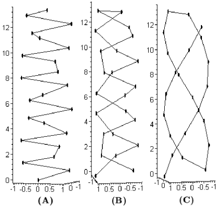
Figure 1: (A) The sequence $n=23$, $k=1$, $j=0$; (B) The union of the sequences $n=23$, $k=2$, $j=0$ and $n=23$, $k=2$, $j=1$; (C) The union of the sequences $n=23$, $k=3$, $j=0$; $n=23$, $k=3$, $j=1$ and $n=23$, $k=3$, $j=2$.

In the following, we take $M$ to be the $\bbbr^{3}$ manifold with an Euclidean definition of distance, or $E^{3}$.

The coordinates of the points $P_{j+kl}$ are given analogously to (3.1). The Euclidean length of $n-$point configurations like those of Fig.1 above can be written,

$$l_{\mathrm{SP}}(k,\omega,\alpha)=(n-k)\sqrt{k^{2}\alpha^{2}\omega^{2}+A_{k}+1}+(k-1)\sqrt{\alpha^{2}\omega^{2}+A_{1}+1}$$ (3.11)

where

$$A_{k}=1-2\cos(k\omega)\enspace.$$ (3.12)

There is only one Steiner Tree for all these point configurations. It has the 3-sausage’s topology [10] and its Euclidean length [6, 3, 11] is written as

$$l_{ST}(\omega,\alpha)=(n-2)(1-r)+(n-3)\alpha\omega\sqrt{\frac{A_{1}+1}{A_{1}}}+2\sqrt{\alpha^{2}\omega^{2}+(1-r)^{2}+r(A_{1}+1)}$$ (3.13)

where

$$r(\omega,\alpha)=\frac{\alpha\omega}{\sqrt{A_{1}(A_{1}+1)}}\enspace.$$ (3.14)

The Steiner points are also in a helix of the same pitch but smaller radius $r(\omega,\alpha)$ as compared to the points of the configuration (3.1).

In order to adapt the formulae (2.1) and (2.2) to the present case of a SRF definition we should note that if we take $n\gg k$, all the sets $A\subset E^{3}$ should be considered as the same. This is a set of a great number of points evenly spaced in a right circular helix.

For $n\gg k$, we then have, from (2.2), (3.13) and (3.14),

$$l_{\mathrm{SMT}}(\omega,\alpha)=n\left(1+\alpha\omega\sqrt{\frac{A_{1}}{A_{1}+1}}\right)$$ (3.15)

and from (2.1), (3.11) and (3.12),

$$l_{\mathrm{MST}}(k,\omega,\alpha)=n\sqrt{k^{2}\alpha^{2}\omega^{2}+A_{k}+1}\enspace.$$ (3.16)

The Steiner Ratio Function is now defined, according (2.3), (3.15) and (3.16) as

$$\rho(\omega,\alpha)=\frac{1+\alpha\omega\sqrt{\frac{A_{1}}{A_{1}+1}}}{\underset{k}{\min}\left(\sqrt{k^{2}\alpha^{2}\omega^{2}+A_{k}+1}\right)}\enspace.$$ (3.17)

The “$\underset{k}{\min}$” in the equation above should be understood in the sense of a new function formed in a piecewise way from the functions corresponding to the chosen $k-$values. For $k=1,2,3$ this means

$$\min\left(\sqrt{\alpha^{2}\omega^{2}+A_{1}+1},\sqrt{4\alpha^{2}\omega^{2}+A_{2}+1},\sqrt{9\alpha^{2}\omega^{2}+A_{3}+1}\right)\enspace.$$

The associated Steiner Ratio for these helical point configurations will be given by the Global minimum of the function $\rho(\omega,\alpha)$ above, according (2.4).

4 The Fitting of Computational Results of the W. D. Smith’s Algorithm

In Fig.2 below, we represent a section of the SRF given by (3.17) for $\alpha=\alpha_{\mathrm{R}}=0.26454000216\ldots$. This is the pitch of a helical configuration in which the points are regular tetrahedra vertices. These tetrahedra are glued together at common faces to form a 3-sausage configuration [12]. The condition for equal edges of the tetrahedra lead to the following equations:

$$\alpha\omega=\frac{\sqrt{3}}{3}\sqrt{A_{1}-A_{2}},$$ (4.1)

$$\alpha\omega=\frac{\sqrt{5}}{5}\sqrt{A_{2}-A_{3}},$$ (4.2)

$$\alpha\omega=\frac{\sqrt{2}}{4}\sqrt{A_{1}-A_{3}}.$$ (4.3)

Only two of them are independent and the non-trivial solution is

$$\omega=\pi-\arccos\left(\frac{2}{3}\right)=2.30052398302\ldots,\,\,\,\alpha=\frac{\sqrt{30}}{9(\pi-\arccos\left(\frac{2}{3}\right))}=0.26454000216\ldots$$ (4.4)

We take $k=1,2,3$ and the points obtained from the W. D. Smith’s algorithm [7] with a search space reduction, i.e., adopting the 3-sausage’s topology as the only feasible. The modified algorithm is available at the site www.biomat.org.

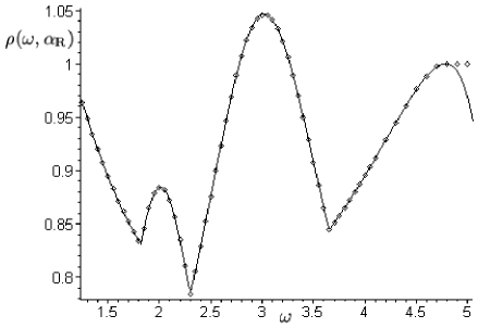
Figure 2: The section $\alpha=\alpha_{\mathrm{R}}$ of the surface $\rho(\omega,\alpha)$ (— ) for $k=1,2,3$ with points obtained from computing experiments ($\diamond$).

It should be noted from Fig.2 that the function (3.17) is a very good fitting to the experiments which were done with the W. D. Smith’s algorithm. It is so a good fitting, that it has the same bad performance at some $\omega-$region $(\rho>1!)$ as can be seem in Fig.2 above. Although these can be easily explained by the difficulty of working with a quasi-plane configuration (the neighbourhood of $\omega=\pi$) when we choose a priori 3-dimensional configurations, we prefer to circumvent this difficulty in the next section. We do it by introducing some necessary restrictions related to Full Steiner Trees.

From the viewpoint of the search of a Global minimum, the surface given by (3.17) is also a very good candidate as can be seen from its level curves in Fig.3 below

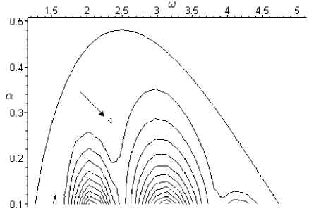
Figure 3: Level curves of the surface $\rho(\omega,\alpha)$, (3.17). The region which contains the projection of the Global minimum point is pointed out by the arrow.

If we substitute into (3.17) the values $(\omega,\alpha)$ corresponding to the 3-sausage’s configuration, or $\omega=\pi-\arccos(2/3)$, $\alpha=\sqrt{30}/9(\pi-\arccos(2/3))$, we get

$$\rho=\frac{1}{10}(3\sqrt{3}+\sqrt{7})=0.78419037337\ldots$$ (4.5)

which is the value given by the authors of [12] for the best upper value for the Steiner Ratio of the $E^{3}$-manifold.

5 The Restriction to Full Steiner Trees

In the last section there is no restriction to Full Steiner Trees. We take as an assumption that the natural organization of biomacromolecular structure is biased by Full Steiner Trees. A structure is non-degenerate or it is almost completely degenerate. Nature can provide a process in which the Steiner Ratio is approaching continuously to the value $\rho=1$. However, the tree cannot be partially degenerate in the sense of partial full trees connected at degenerate vertices.

In this section, we emphasize that we need more stringent constraints, instead of a constraint relaxation for a good definition of SRF. “Good” means here the definition which leads to $\rho-$values lesser than the value reported in Section 4 if we believe that the main conjecture of the authors of [8] could be disproved.

If we look at Fig.2 above, we can see that the algorithm used as well as the modelling based on (3.17) do not make any discrimination to degenerate Steiner Trees. This is due to the fact that there are regions of $\omega$-values in which $\rho$ is close to 1. To each $(\omega,\alpha)$ pair of values there is associated a point configuration. This means that there are regions in the line $(\omega,\alpha_{\mathrm{R}})$ corresponding to degenerate configurations. This is also valid for other $\alpha-$values since these sections of the surface (3.17) have similar profiles.

We can now introduce the restriction to full Steiner Trees. Let us take the $j$, $k$ subsequence of (3.4). The points $P_{j},P_{j+k},P_{j+2k},\ldots$ are evenly spaced along the corresponding right circular helix. The angle made by contiguous edges is

$$\cos{\theta_{k}}=\frac{\overrightarrow{P_{j+lk}P_{j+(l+1)k}}\cdot\overrightarrow{P_{j+(l+2)k}P_{j+(l+1)k}}}{\|\overrightarrow{P_{j+lk}P_{j+(l+1)k}}\|\|\overrightarrow{P_{j+(l+2)k}P_{j+(l+1)k}}\|}$$ (5.1)

where $\|\cdot\|$ is the Euclidean norm.

The cartesian coordinates of the points $P_{j+kl}$ can be written analogously to (3.1) and we have

$$\cos{\theta_{k}}=-1+\frac{(A_{k}+1)^{2}}{2(k^{2}\alpha^{2}\omega^{2}+A_{k}+1)}$$ (5.2)

where $A_{k}$ is given by (3.12).

The restrictions to Full Steiner Trees can be then written in the form

$$\cos{\theta_{k}}\geq-\frac{1}{2}\enspace.$$ (5.3)

In Fig.4 below we show the restrictions introduced by (5.3) for $k=1,2,3$. The horizontal line corresponds to the value $\cos{\theta_{k}}=-1/2$.

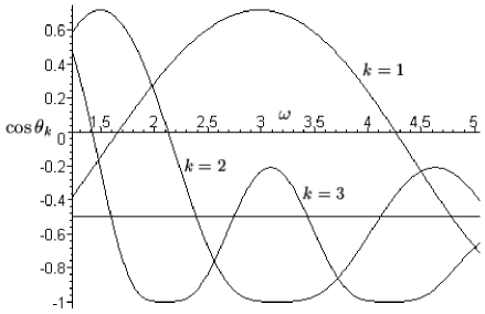
Figure 4: The restriction to Full Steiner Trees. The figure is a section of the surfaces (5.2) for $\alpha=\alpha_{\mathrm{R}}$.

The spanning trees corresponding to $k=2$ have a large forbidden region. The $k=1$ curve is the only one which corresponds to Full Steiner Trees in a large region of the $\omega-$interval studied in this work. The proposal for the Steiner Ratio Function is given in this case by

$$\rho_{1}(\omega,\alpha)=\frac{l_{\mathrm{SMT}}(\omega,\alpha)}{l_{\mathrm{MST}}(1,\omega,\alpha)}\enspace.$$ (5.4)

From (3.17), we get

$$\rho_{1}(\omega,\alpha)=\frac{1+\alpha\omega\sqrt{\frac{A_{1}}{A_{1}+1}}}{\sqrt{\alpha^{2}\omega^{2}+A_{1}+1}}\enspace.$$ (5.5)

Fig.5 shows the sections $\alpha=\alpha_{\mathrm{R}}$ of the surfaces given by (3.17) and (5.5). By restricting our observations to the $\omega-$interval in which the $k=1$ curve in Fig.4 allows for Full Steiner Trees, it should be noted that the section $\alpha=\alpha_{\mathrm{R}}$ of the candidate for a SRF given by (5.5) is the convex envelope [13] of the section $\rho(\omega,\alpha_{\mathrm{R}})$ of (3.17).

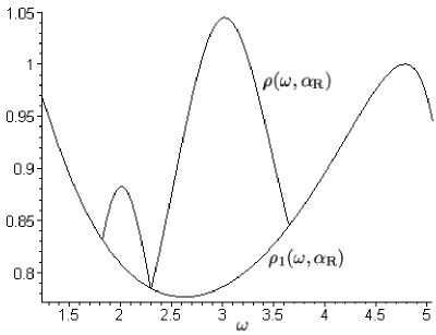
Figure 5: The $\rho_{1}(\omega,\alpha_{\mathrm{R}})$ candidate is a convex envelope of the function $\rho(\omega,\alpha_{\mathrm{R}})$.

6 Concluding Remarks

The restriction of the point configurations only to those which lead to Full Steiner Trees, has wiped out the Global minima of the surface $\rho(\omega,\alpha)$. The resulting surface $\rho_{1}(\omega,\alpha)$ satisfies the necessary bounds [3]

$$\frac{1}{2}\leq\rho_{1}(\omega,\alpha)\leq 1$$ (6.1)

in the $\omega-$interval

$$\arccos\left(\frac{1}{3}\right)\leq\omega\leq 2\pi-\arccos\left(\frac{1}{3}\right)$$ (6.2)

If we wish to restrict the $\rho$-values by using the Du-Hwang’s greatest lower bound $(\rho=\sqrt{3}/3)$ instead of Moore’s $(\rho=1/2)$, we have to substitute (6.2) by

$$\arccos\left(\frac{1}{4}\right)\leq\omega\leq 2\pi-\arccos\left(\frac{1}{4}\right)$$ (6.3)

We need a constraint to be motivated by the natural organization of a macromolecular structure in our modelling. Some interesting results have been obtained [4] by introducing a function of the form

$$H(\omega,\alpha)=(1+\lambda)\rho_{1}(\omega,\alpha)-\lambda\phi(\omega,\alpha)$$ (6.4)

where $\lambda$ is a Lagrange multiplier and $\phi(\omega,\alpha)$ stands for a recently proposed function for chirality measure [4] given by

$$\phi(\omega,\alpha)=\frac{1}{6}\alpha\omega\sin(\omega)\left(\frac{A_{1}+1}{A_{1}}\right)(\alpha^{2}\omega^{2}-A_{1}(A_{1}+1)).$$ (6.5)

The work with (6.4) has produced a new upper bound for $\rho_{1}(\omega,\alpha)$ which is still lower than the unconstrained minimum of $\rho_{1}(\omega,\alpha_{\mathrm{R}})$ as compared to the Global minimum value of $\rho(\omega,\alpha)$.

It would be easy to announce a proof for the conjecture of [12] or at least some very good arguments for a proof from the work of the last sections. However, in spite of the evidences which were reported here, we think that the approach adopted has given nice advances in our program of modelling the structure of biomacromolecules with Steiner Points and Steiner Trees. The possibility of analyzing the chirality effects on these structures is one of these advances.

References

- [1] Smith, J. M.: Steiner Minimal Trees in : Theory, Algorithms and Applications. Handbook of Combinatorial Optimization 2, Kluwer Acad. Publ. (1998) 397–470.
- [2] Mondaini, R. P.: The Minimal Surface Structure of Biomolecules. Proceedings of the First Brazilian Symposium on Mathematical and Computational Biology – ed. E-papers LTDA, Rio de Janeiro (2001) 1–11.
- [3] Mondaini, R. P.: The Disproof of a Conjecture on the Steiner Ratio in and its Consequences for a Full Geometric Description of Macromolecular Chirality. Proceedings of the Second Brazilian Symposium on Mathematical and Computational Biology – ed. E-papers LTDA, Rio de Janeiro (2002) 101–177.
- [4] Mondaini, R. P.: Proposal for Chirality Measure as the Constraint of a Constrained Optimization Problem. Proceedings of the Third Brazilian Symposium on Mathematical and Computational Biology – ed. E-papers LTDA, Rio de Janeiro (2004) 65–74.
- [5] Mondaini, R. P.: The Geometry of Macromolecular Structure: Points and Steiner Trees. Proceedings of the Fourth Brazilian Symposium on Mathematical and Computational Biology – ed. E-papers LTDA, Rio de Janeiro (2005).
- [6] Mondaini, R. P.: The Steiner Ratio and the Homochirality of Biomacromolecular Structures. Frontiers in Global Optimization: Nonconvex Optimization and its Applications Series 74, Kluwer Acad. Publ. (2003) 373–390.
- [7] Smith, W. D.: How to find Steiner Minimal Trees in Euclidean Space. Algorithmica 7 (1992) 137–177.
- [8] Smith, W. D., MacGregor Smith, J.: The Steiner Ratio in 3D Space. Journ. Comb. Theory A69 (1995) 301–332.
- [9] Mondaini, R. P.: The Euclidean Steiner Ratio and the Measure of Chirality of Biomacromolecules. Genetics and Molecular Biology, vol.27, 4 (2004) 658–664.
- [10] Smith, J. M., Toppur, B.: Euclidean Steiner Minimal Trees, Minimal Energy Configurations, and the Embedding Problem of Weighted Graphs in . Discret. Appl. Math. 71 (1996) 187–215.
- [11] Mondaini, R. P., Oliveira, N. V.: The State of Art on the Steiner Ratio Value in . Tendências em Matemática Aplicada e Computacional, vol.5, 2 (2004).
- [12] Du, D. Z., Smith, W. D.: Disproofs of the Generalized Gilbert-Pollak Conjecture on the Steiner Ratio in Three or more Dimensions. Journ. Comb. Theory A74 (1996) 115–130.
- [13] Bazaraa, M. S., Sherali, H. D., Shetty, C. M.: Nonlinear Programming. Wiley (1993) pp.125.