Strong resonant tunneling, level repulsion and spectral type for one-dimensional adiabatic quasi-periodic Schrödinger operators

Abstract.

In this paper, we consider one dimensional adiabatic quasi-periodic Schrödinger operators in the regime of strong resonant tunneling. We show the emergence of a level repulsion phenomenon which is seen to be very naturally related to the local spectral type of the operator: the more singular the spectrum, the weaker the repulsion.

Résumé. Dans cet article, nous étudions une famille d’opérateurs quasi-périodiques adiabatiques dans un cas d’effet tunnel résonant fort. Nous voyons l’apparition d’un phénomène de répulsion de niveaux fort qui est relié au type spectral local de l’opérateur : plus le spectre est singulier, plus la répulsion est faible.

0. Introduction

In [3], we studied the spectrum of the family of one-dimensional quasi-periodic Schrödinger operators acting on $L^{2}({\mathbb{R}})$ and defined by

(0.1) $$H_{z,\varepsilon}\psi=-\frac{d^{2}}{dx^{2}}\psi(x)+(V(x-z)+\alpha\cos(\varepsilon x))\psi(x),$$

where

(H1):

$V:\ {\mathbb{R}}\to{\mathbb{R}}$ is a non constant, locally square integrable, $1$-periodic function;

(H2):

$\varepsilon$ is a small positive number chosen such that $2\pi/\varepsilon$ be irrational;

(H3):

$z$ is a real parameter indexing the operators;

(H4):

$\alpha$ is a strictly positive parameter that we will keep fixed in most of the paper.

To describe the energy region where we worked, consider the spectrum of the periodic Schrödinger operator (on $L^{2}({\mathbb{R}})$)

(0.2) $$H_{0}=-\frac{d^{2}}{dx^{2}}+V\,(x)$$

Figure 1. Bands in interaction

We assumed that two of its spectral bands are interacting through the perturbation $\alpha\cos$ i.e., that the relative position of the spectral window $\mathcal{F}(E):=[E-\alpha,E+\alpha]$ and the spectrum of the unperturbed operator $H_{0}$ is that shown in Fig. 1. In such an energy region, the spectrum is localized near two sequences of quantized energy values, say $(E_{0}^{(l)})_{l}$ and $(E_{\pi}^{(l^{\prime})})_{l}^{\prime}$ (see Theorem 1.1); each of these sequences is “generated” by one of the ends of the neighboring spectral bands of $H_{0}$. In [3], we restricted our study to neighborhoods of such quantized energy values that were not resonant i.e. to neighborhoods of the points $E_{\mu}^{(l)}$ that were not “too” close to the points $(E_{\nu}^{(l^{\prime})})_{l}^{\prime}$ for $\{\mu,\nu\}=\{0,\pi\}$. Already in this case, the distance between the two sequences influences the nature and location of the spectrum: we saw a weak level repulsion arise “due to weak resonant tunneling”.
Similarly to what happens in the standard “double well” case (see [20, 10]), the resonant tunneling begins to play an important role when the two energies, each generated by one of the quantization conditions, are sufficiently close to each other. In the present paper, we deal with the resonant case, i.e. the case when two of the “interacting energies” are “very” close to each other or even coincide. We find a strong relationship between the level repulsion and the nature of the spectrum. Recall that the latter is determined by the speed of decay of the solutions to $(H_{z,\varepsilon}-E)\psi=0$ (see [9]). Expressed in this way, it is very natural that the two characteristics are related: the slower the decay of the generalized eigenfunctions, the larger the overlap between generalized eigenfunction corresponding to close energy levels, hence, the larger the tunneling between these levels and thus the repulsion between them.

Let us now briefly describe the various situations we encounter. Therefore, we briefly recall the settings and results of [3]. Let $J$ be an interval of energies such that, for all $E\in J$, the spectral window $\mathcal{F}(E)$ covers the edges of two neighboring spectral bands of $H_{0}$ and the gap located between them (see Fig. 1 and assumption (TIBM)). Under this assumption, consider the real and complex iso-energy curves associated to (0.1). Denoted respectively by $\Gamma_{\mathbb{R}}$ and $\Gamma$, they are defined by

(0.3) $$\Gamma_{\mathbb{R}}:=\{(\kappa,\zeta)\in{\mathbb{R}}^{2},\ \mathbf{E}(\kappa)+\alpha\cdot\cos(\zeta)=E\},$$

(0.4) $$\Gamma:=\{(\kappa,\zeta)\in{\mathbb{C}}^{2},\ \mathbf{E}(\kappa)+\alpha\cdot\cos(\zeta)=E\}.$$

where $\mathbf{E}(\kappa)$ be the dispersion relation associated to $H_{0}$ (see section 1.1.2). These curves are roughly depicted in Fig. 2. They are periodic both in $\zeta$ and $\kappa$ directions.

Consider one of the periodicity cells of $\Gamma_{\mathbb{R}}$. It contains two tori. They are denoted by $\gamma_{0}$ and $\gamma_{\pi}$

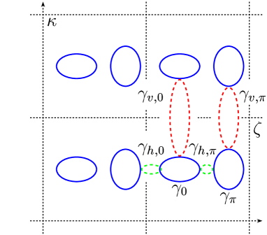
Figure 2. The adiabatic phase space

and shown in full lines. To each of them, one associates a phase obtained by integrating $1/2$ times the fundamental $1$-form on $\Gamma$ along the tori; we denote the phases by $\Phi_{0}$ and $\Phi_{\pi}$ respectively (see section 1.3).
Each of the dashed lines in Fig. 2 represents a loop on $\Gamma$ that connects certain connected components of $\Gamma_{\mathbb{R}}$; one can distinguish between the “horizontal” loops and the “vertical” loops. There are two special horizontal loops denoted by $\gamma_{h,0}$ and $\gamma_{h,\pi}$; the loop $\gamma_{h,0}$ (resp. $\gamma_{h,\pi}$) connects $\gamma_{0}$ to $\gamma_{\pi}-(2\pi,0)$ (resp. $\gamma_{0}$ to $\gamma_{\pi}$). In the same way, there are two special vertical loops denoted by $\gamma_{v,0}$ and $\gamma_{v,\pi}$ ; the loop $\gamma_{v,0}$ (resp. $\gamma_{v,\pi}$) connects $\gamma_{0}$ to $\gamma_{0}+(0,2\pi)$ (resp. $\gamma_{\pi}$ to $\gamma_{\pi}+(0,2\pi)$). To each of these complex loops, one associates an action obtained by integrating $-i/2$ times the fundamental $1$-form on $\Gamma$ along the loop. For $a\in\{0,\pi\}$ and $b\in\{v,h\}$, we denote by $S_{a,b}$ the action associated to $\gamma_{a,b}$. For $E$ real, all these actions are real. One orients the loops so that they all be positive. Finally, we define tunneling coefficients as

$$t_{a,b}=e^{-S_{a,b}/\varepsilon},\quad a\in\{0,\pi\},\ b\in\{v,h\}.$$

Each of the curves $\gamma_{0}$ and $\gamma_{\pi}$ defines a sequence of “quantized energies” in $J$ (see Theorem 1.1). They satisfy the “quantization” conditions

(0.5) $$\frac{1}{\varepsilon}\Phi_{0}(E_{0}^{(l)})=\frac{\pi}{2}+l\pi+o(1),\quad l\in{\mathbb{Z}},\quad\quad\frac{1}{\varepsilon}\check{\Phi}_{\pi}(E_{\pi}^{(m)})=\frac{\pi}{2}+m\pi+o(1),\quad m\in{\mathbb{Z}},$$

where $o(1)$ denote real analytic functions of $E$ that are small for small $\varepsilon$. By Theorem 1.1, for $a\in\{0,\pi\}$, near each $E_{a}^{(l)}$, there is one exponentially small interval $I_{a}^{(l)}$ such that the spectrum of $H_{z,\varepsilon}$ in $J$ is contained in the union of all these intervals. The precise description of the spectrum in the interval $I_{a}^{(l)}$ depends on whether it intersects another such interval or not. Note that an interval of type $I_{0}^{(l)}$ can only intersect intervals of type $I_{\pi}^{(l)}$ and vice versa (see section 1.3.3).

The paper [3] was devoted to the study of the spectrum in intervals $I_{a}^{(l)}$ that do not intersect any other interval. In the present paper, we consider two intervals $I_{0}^{(l)}$ and $I_{\pi}^{(l^{\prime})}$ that do intersect and describe the spectrum in the union of these two intervals. It is useful to keep in mind that this union is exponentially small (when $\varepsilon$ goes to $0$).

There are two main parameters controlling the spectral type:

$$\tau=2\sqrt{\frac{t_{v,0}\,t_{v,\pi}}{t_{h,0}\,t_{h,\pi}}}\quad\quad\quad\text{and}\quad\quad\quad\rho=2\sqrt{\frac{\max(t_{v,0},t_{v,\pi})^{2}}{t_{h,0}\,t_{h,\pi}}}$$

Here, as we are working inside an exponentially small interval, the point inside this interval at which we compute the tunneling coefficients does not really matter: over this interval, the relative variation of any of the actions is exponentially small.
Noting that $\rho\geq\tau$, we distinguish three regimes:

• $\tau\gg 1$,

• $\rho\gg 1$ and $\tau\ll 1$,

• $\rho\ll 1$.

Here, the symbol $\gg 1$ (resp. $\ll 1$) mean that the quantity is exponentially large (resp. small) in $\frac{1}{\varepsilon}$ as $\varepsilon$ goes to $0$, the exponential rate being arbitrary, see section 1.5.
In each of the three cases, we consider two energies, say $E_{0}$ and $E_{\pi}$, satisfying respectively the first and the second relation in (0.5), and describe the evolution of the spectrum as $E_{0}$ and $E_{\pi}$ become closer to each other. As explained in Remark 1.2 in [3], this can be achieved by reducing $\varepsilon$ somewhat. As noted above, when moving these two energies, we can consider that the other parameters in the problem, mainly the tunneling coefficients, hence, the coupling constants $\tau$ and $\rho$ stay constant; in particular, we stay in one of the three cases described above when we move $E_{0}$ and $E_{\pi}$ closer together.

Assume we are in the case $\tau\gg 1$. Then, when $E_{0}$ and $E_{\pi}$ are still “far” away from each other, one sees two intervals containing spectrum (sub-intervals of the corresponding intervals $I_{0}$ and $I_{\pi}$), one located near each energy; they contain the same amount of spectrum i.e. the measure with respect to the density of states of each interval is $\varepsilon/2\pi$; and the Lyapunov exponent is positive on both intervals (see Fig. 5(a)). When $E_{0}$ and $E_{\pi}$ approach each other, at some moment these two intervals merge into one, so only a single interval is seen (see Fig. 5(b)); its density of states measure is $\varepsilon/\pi$ and the Lyapunov exponent is still positive on this interval. There is no gap separating the intervals of spectrum generated by the two quantization conditions . This can be interpreted as a consequence of the positivity of the Lyapunov exponent : the states are well localized so the overlapping is weak and there no level repulsion. Nevertheless, the resonance has one effect: when the two intervals merge, it gives rise to a sharp drop of the Lyapunov exponent (which still stays positive) in the middle of the interval containing spectrum. Over a distance exponentially small in $\varepsilon$, the Lyapunov exponent drops by an amount of order one.

In the other extreme, in the case $\rho\ll 1$, the “starting” geometry of the spectrum is the same as in the previous case, namely, two well separated intervals containing each an $\varepsilon/2\pi$ “part” of spectrum. When these intervals become sufficiently close one to another most of the spectrum on these intervals is absolutely continuous (even if the spectrum was singular when the intervals were “far” enough). As the energies $E_{0}$ and $E_{\pi}$ approach each other, so do the intervals until they roughly reach an interspacing of size $\sqrt{t_{h}}$; during this process, the sizes of the intervals which, at the start, were roughly of order $t_{v,0}+t_{h}$ and $t_{v,\pi}+t_{h}$ grew to reach the order of $\sqrt{t_{h}}$ (this number is much larger than any of the other two as $\rho\ll 1$). When $E_{0}$ and $E_{\pi}$ move closer to each other, the intervals containing the spectrum stay “frozen” at a distance of size $\sqrt{t_{h}}$ from each other, and their sizes do not vary noticeably either (see Fig. 6). They start moving and changing size again when $E_{0}$ and $E_{\pi}$ again become separated by an interspacing of size at least $\sqrt{t_{h}}$. So, in this case, we see a very strong repulsion preventing the intervals of spectra from intersecting each other. The spacing between them is quite similar to that observed in the case of the standard double well problem (see [20, 10]).

In the last case, when $\rho\gg 1$ and $\tau\ll 1$, we see an intermediate behavior. For the sake of simplicity, let us assume that $t_{v,\pi}\gg t_{v,0}$. Starting from the situation when $E_{0}$ and $E_{\pi}$ are “far” apart, we see two intervals, one around each point $E_{0}$ and $E_{\pi}$ and this as long as $|E_{0}-E_{\pi}|\gg t_{v,\pi}$ (see Fig. 7(a)). When $|E_{0}-E_{\pi}|$ becomes roughly of size $t_{v,\pi}$ or smaller, as in the first case, the Lyapunov exponent varies by an amount of order one over each of the exponentially small intervals. The difference is that it need not stay positive: at the edges of the two intervals that are facing each other, it becomes small and even can vanish. These are the edges that seem more prone to interaction. Now, when one moves $E_{0}$ towards $E_{\pi}$, the lacuna separating the two intervals stays open and starts moving with $E_{0}$; it becomes roughly centered at $E_{0}$, stays of fixed size (of order $t_{h}/t_{v,\pi}$) and moves along with $E_{0}$ as $E_{0}$ crosses $E_{\pi}$ and up to a distance roughly $t_{v,\pi}$ on the other side of $E_{\pi}$ (see Fig. 7(b)). Then, when $E_{0}$ moves still further away from $E_{\pi}$, it becomes again the center of some interval containing spectrum that starts moving away from the band centered at $E_{\pi}$. We see that, in this case as in the case of strong repulsion, there always are two intervals separated by a gap; both intervals contain a $\varepsilon/2\pi$ “part” of spectrum. But, now, the two intervals can become exponentially larger than the gap (in the case of strong interaction, the length of the gap was at least of the same order of magnitude as the lengths of the bands). Moreover, on both intervals, the Lyapunov exponent is positive near the outer edges i.e. the edges that are not facing each other; it can become small or even vanish on the inner edges. So, there may be some Anderson transitions within the intervals. We see here the effects of a weaker form of resonant tunneling and a weaker repulsion.

To complete this introduction, let us note that, though in the present paper we only considered a perturbation given by a cosine, it is clear from our techniques that the same phenomena appear as long as the phase space picture is that given in Fig. 2.

1. The results

We now state our assumptions and results in a precise way.

1.1. The periodic operator

This section is devoted to the description of elements of the spectral theory of one-dimensional periodic Schrödinger operator $H_{0}$ that we need to present our results. For more details and proofs, we refer to section 6 and to [2, 8].

1.1.1. The spectrum of $H_{0}$

The spectrum of the operator $H_{0}$ defined in (0.2) is a union of countably many intervals of the real axis, say $[E_{2n+1},\,E_{2n+2}]$ for $n\in{\mathbb{N}}$ , such that

$$E_{1}<E_{2}\leq E_{3}<E_{4}\dots E_{2n}\leq E_{2n+1}<E_{2n+2}\leq\dots\,,$$

$$E_{n}\to+\infty,\quad n\to+\infty.$$

This spectrum is purely absolutely continuous. The points $(E_{j})_{j}$ are the eigenvalues of the self-adjoint operator obtained by considering the differential polynomial (0.2) acting in $L^{2}([0,2])$ with periodic boundary conditions (see [2]). For $n\in{\mathbb{N}}$, the intervals $[E_{2n+1},\,E_{2n+2}]$ are the spectral bands, and the intervals $(E_{2n},\,E_{2n+1})$, the spectral gaps. When $E_{2n}<E_{2n+1}$, one says that the $n$-th gap is open; when $[E_{2n-1},E_{2n}]$ is separated from the rest of the spectrum by open gaps, the $n$-th band is said to be isolated. Generically all the gap are open.

From now on, to simplify the exposition, we suppose that

(O):

all the gaps of the spectrum of $H_{0}$ are open.

1.1.2. The Bloch quasi-momentum

Let $x\mapsto\psi(x,E)$ be a non trivial solution to the periodic Schrödinger equation $H_{0}\psi=E\psi$ such that $\psi\,(x+1,E)=\mu\,\psi\,(x,E)$, $\forall x\in{\mathbb{R}}$, for some $\mu\in{\mathbb{C}}^{*}$ independent of $x$. Such a solution is called a Bloch solution to the equation, and $\mu$ is the Floquet multiplier associated to $\psi$. One may write $\mu=\exp(ik)$ where, $k$ is the Bloch quasi-momentum of the Bloch solution $\psi$.

It appears that the mapping $E\mapsto k(E)$ is analytic and multi-valued; its branch points are the points $\{E_{n};\ n\in{\mathbb{N}}\}$. They are all of “square root” type.

The dispersion relation $k\mapsto{\mathbf{E}}(k)$ is the inverse of the Bloch quasi-momentum. We refer to section 6.1.2 for more details on $k$.

1.2. A “geometric” assumption on the energy region under study

Let us now describe the energy region where our study is valid.

Recall that the spectral window $\mathcal{F}(E)$ is the range of the mapping $\zeta\in{\mathbb{R}}\mapsto E-\alpha\cos(\zeta)$.

In the sequel, $J$ always denotes a compact interval such that, for some $n\in{\mathbb{N}}^{*}$ and for all $E\in J$, one has

(TIBM):

$[E_{2n},E_{2n+1}]\subset\dot{\mathcal{F}}(E)$ and ${\mathcal{F}}(E)\subset]E_{2n-1},E_{2n+2}[$.

where $\dot{\mathcal{F}}(E)$ is the interior of $\mathcal{F}(E)$ (see figure 1).

Remark 1.1.

As all the spectral gaps of $H_{0}$ are assumed to be open, as their length tends to $0$ at infinity, and, as the length of the spectral bands goes to infinity at infinity, it is clear that, for any non vanishing $\alpha$, assumption (TIBM) is satisfied in any gap at a sufficiently high energy; it suffices that this gap be of length smaller than $2\alpha$.

1.3. The definitions of the phase integrals and the tunneling coefficients

We now give the precise definitions of the phase integrals and the tunneling coefficients introduced in the introduction.

1.3.1. The complex momentum and its branch points

The phase integrals and the tunneling coefficients are expressed in terms of integrals of the complex momentum. Fix $E$ in $J$. The complex momentum $\zeta\mapsto\kappa(\zeta)$ is defined by

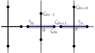
Figure 3. The branch points

(1.1) $$\hskip-113.81102pt\kappa(\zeta)=k(E-\alpha\cos(\zeta)).$$

As $k$, $\kappa$ is analytic and multi-valued. The set $\Gamma$ defined in (0.4) is the graph of the function $\kappa$. As the branch points of $k$ are the points $(E_{i})_{i\in{\mathbb{N}}}$, the branch points of $\kappa$ satisfy

(1.2) $$\hskip-113.81102ptE-\alpha\cos(\zeta)=E_{j},\ j\in{\mathbb{N}}^{*}.$$

As $E$ is real, the set of these points is symmetric with respect to the real axis and to the imaginary axis, and it is
$2\pi$-periodic in $\zeta$. All the branch points of $\kappa$ lie on $\arccos({\mathbb{R}})$. This set consists of the real axis and all the translates of the imaginary axis by a multiple of $\pi$. As the branch points of the Bloch quasi-momentum, the branch points of $\kappa$ are of “square root” type. Due to the symmetries, it suffices to describe the branch points in the half-strip $\{\zeta;\ {\rm Im}\,\zeta\geq 0,\ 0\leq{\rm Re}\,\zeta\leq\pi\}$. These branch points are described in detail in section 7.1.1 of [3]. In figure 3, we show some of them. The points $\zeta_{j}$ being defined by (1.2), one has $0<\zeta_{2n}<\zeta_{2n+1}<\pi$, $0<{\rm Im}\,\zeta_{2n+2}<{\rm Im}\,\zeta_{2n+3}<\cdots$, $0<{\rm Im}\,\zeta_{2n-1}<\cdots<{\rm Im}\,\zeta_{1}$.

1.3.2. The contours

To define the phases and the tunneling coefficients, we introduce some integration contours in the complex $\zeta$-plane.
These loops are shown in figures 3 and 4. The loops $\tilde{\gamma}_{0}$, $\tilde{\gamma}_{\pi}$, $\tilde{\gamma}_{h,0}$, $\tilde{\gamma}_{h,\pi}$, $\tilde{\gamma}_{v,0}$ and $\tilde{\gamma}_{v,\pi}$ are simple loops, respectively, going once around the intervals $[-\zeta_{2n},\zeta_{2n}]$, $[\zeta_{2n+1},2\pi-\zeta_{2n+1}]$, $[-\zeta_{2n+1},-\zeta_{2n}]$, $[\zeta_{2n},\zeta_{2n+1}]$, $[\zeta_{2n-1},\overline{\zeta_{2n-1}}]$ and $[\zeta_{2n+2},\overline{\zeta_{2n+2}}]$.
In section 10.1 of [3], we have shown that, on each of the above loops, one can fix a continuous branch of the complex momentum.
Consider $\Gamma$, the complex iso-energy curve defined by (0.4). Define the projection $\Pi:(\zeta,\kappa)\in\Gamma\mapsto\zeta\in{\mathbb{C}}$. As on each of the loops $\tilde{\gamma}_{0}$, $\tilde{\gamma}_{\pi}$, $\tilde{\gamma}_{h,0}$, $\tilde{\gamma}_{h,\pi}$, $\tilde{\gamma}_{v,0}$ and $\tilde{\gamma}_{v,\pi}$, one can fix a continuous branch of the complex momentum, each of these loops is the projection on the complex plane of some loop in $\Gamma$. In sections 10.6.1 and 10.6.2 of [3], we give the precise definitions of the curves $\gamma_{0}$, $\gamma_{\pi}$, $\gamma_{h,0}$, $\gamma_{h,\pi}$, $\gamma_{v,0}$ and $\gamma_{v,\pi}$ represented in figure 2 and show that they respectively project onto the curves $\tilde{\gamma}_{0}$, $\tilde{\gamma}_{\pi}$, $\tilde{\gamma}_{h,0}$, $\tilde{\gamma}_{h,\pi}$, $\tilde{\gamma}_{v,0}$ and $\tilde{\gamma}_{v,\pi}$.

1.3.3. The phase integrals, the action integrals and the tunneling coefficients

The results described below are proved in section 10 of [3].

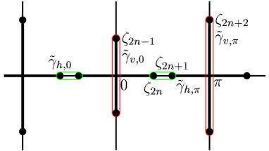
Figure 4. The loops for the action integrals

Let $\nu\in\{0,\pi\}$. To the loop $\gamma_{\nu}$, we associate the phase integral $\Phi_{\nu}$ defined as

(1.3) $$\hskip-142.26378pt\Phi_{\nu}(E)=\frac{1}{2}\oint_{\tilde{\gamma}_{\nu}}\kappa\,d\zeta,$$

where $\kappa$ is a branch of the complex momentum that is continuous on $\tilde{\gamma}_{\nu}$. The function $E\mapsto\Phi_{\nu}(E)$ is real analytic and does not vanish on $J$. The loop $\tilde{\gamma}_{\nu}$ is oriented so that $\Phi_{\nu}(E)$ be positive. One shows that, for all $E\in J$,

(1.4) $$\hskip-142.26378pt\quad\Phi_{0}^{\prime}(E)<0\quad\text{ and }\quad\Phi_{\pi}^{\prime}(E)>0.$$

To the loop $\gamma_{v,\nu}$, we associate the vertical action integral $S_{v,\nu}$ defined as

(1.5) $$S_{v,\nu}(E)=-\frac{i}{2}\oint_{\tilde{\gamma}_{v,\nu}}\kappa d\zeta,$$

where $\kappa$ is a branch of the complex momentum that is continuous on $\tilde{\gamma}_{v,\nu}$. The function $E\mapsto S_{v,\nu}(E)$ is real analytic and does not vanish on $J$. The loop $\tilde{\gamma}_{v,\nu}$ is oriented so that $S_{v,\nu}(E)$ be positive.
The vertical tunneling coefficient is defined to be

(1.6) $$t_{v,\nu}(E)=\exp\left(-\frac{1}{\varepsilon}S_{v,\nu}(E)\right).$$

The index $\nu$ being chosen as above, we define horizontal action integral $S_{h,\nu}$ by

(1.7) $$S_{h,\nu}(E)=-\frac{i}{2}\oint_{\tilde{\gamma}_{h,\nu}}\kappa(\zeta)\,d\zeta,$$

where $\kappa$ is a branch of the complex momentum that is continuous on $\tilde{\gamma}_{h,\nu}$. The function $E\mapsto S_{h,\nu}(E)$ is real analytic and does not vanish on $J$. The loop $\tilde{\gamma}_{h,\nu}$ is oriented so that $S_{h,\nu}(E)$ be positive.
The horizontal tunneling coefficient is defined as

(1.8) $$t_{h,\nu}(E)=\exp\left(-\frac{1}{\varepsilon}S_{h,\nu}(E)\right).$$

As the cosine is even, one has

(1.9) $$S_{h,0}(E)=S_{h,\pi}(E)\quad\text{ and }\quad t_{h,0}(E)=t_{h,\pi}(E).$$

Finally, one defines

(1.10) $$S_{h}(E)=S_{h,0}(E)+S_{h,\pi}(E)\quad\text{ and }\quad t_{h}(E)=t_{h,0}(E)\cdot t_{h,\pi}(E).$$

In (1.3), (1.5), and (1.7), only the sign of the integral depends on the choice of the branch of $\kappa$; this sign was fixed by orienting the integration contour.

1.4. A coarse description of the location of the spectrum in $J$

Henceforth, we assume that the assumptions (H) and (O) are satisfied and that $J$ is a compact interval satisfying (TIBM). As in [3], we suppose that

(T):

$\displaystyle 2\pi\cdot\min_{E\in J}\min({\rm Im}\,\zeta_{2n-2}(E),\,{\rm Im}\,\zeta_{2n+3}(E))>\max_{E\in J}\max(S_{h}(E),\,S_{v,0}(E),\,S_{v,\pi}(E))$.

Note that (T) is verified if the spectrum of $H_{0}$ has two successive bands that are sufficiently close to each other and sufficiently far away from the remainder of the spectrum (this can be checked numerically on simple examples, see section 1.8). In section 1.9 of [3], we discuss this assumption further.

Define

(1.11) $$\delta_{0}:=\frac{1}{2}\inf_{E\in J}\min(S_{h}(E),S_{v,0}(E),S_{v,\pi}(E))>0.$$

One has

Theorem 1.1 ([3]).

Fix $E_{*}\in J$. For $\varepsilon$ sufficiently small, there exists $V_{*}\subset{\mathbb{C}}$, a neighborhood of $E_{*}$, and two real analytic functions $E\mapsto\check{\Phi}_{0}(E,\varepsilon)$ and $E\mapsto\check{\Phi}_{\pi}(E,\varepsilon)$, defined on $V_{*}$ satisfying the uniform asymptotics

(1.12) $$\check{\Phi}_{0}(E,\varepsilon)=\Phi_{0}(E)+o(\varepsilon),\quad\check{\Phi}_{\pi}(E,\varepsilon)=\Phi_{\pi}(E)+o(\varepsilon)\quad\text{when }\varepsilon\to 0,$$

such that, if one defines two finite sequences of points in $J\cap V_{*}$, say $(E_{0}^{(l)})_{l}:=(E_{0}^{(l)}(\varepsilon))_{l}$ and $(E_{\pi}^{(l^{\prime})})_{l^{\prime}}:=(E_{\pi}^{(l^{\prime})}(\varepsilon))_{l^{\prime}}$, by

(1.13) $$\frac{1}{\varepsilon}\check{\Phi}_{0}(E_{0}^{(l)},\varepsilon)=\frac{\pi}{2}+\pi l\quad\text{ and }\quad\frac{1}{\varepsilon}\check{\Phi}_{\pi}(E_{\pi}^{(l^{\prime})},\varepsilon)=\frac{\pi}{2}+\pi l^{\prime},\quad(l,\,l^{\prime})\in{\mathbb{N}}^{2},$$

then, for all real $z$, the spectrum of $H_{z,\varepsilon}$ in $J\cap V_{*}$ is contained in the union of the intervals

(1.14) $$I_{0}^{(l)}:=E_{0}^{(l)}+[-e^{-\delta_{0}/\varepsilon},e^{-\delta_{0}/\varepsilon}]\quad\text{ and }\quad I_{\pi}^{(l^{\prime})}:=E_{\pi}^{(l^{\prime})}+[-e^{-\delta_{0}/\varepsilon},e^{-\delta_{0}/\varepsilon}]$$

that is

$$\sigma(H_{z,\varepsilon})\cap J\cap V_{*}\subset\left(\bigcup_{l}I_{0}^{(l)}\right)\bigcup\left(\bigcup_{l^{\prime}}I_{\pi}^{(l^{\prime})}\right).$$

In the sequel, to alleviate the notations, we omit the reference to $\varepsilon$ in the functions $\check{\Phi}_{0}$ and $\check{\Phi}_{\pi}$.

By (1.4) and (1.12), there exists $C>0$ such that, for $\varepsilon$ sufficiently small, the points defined in (1.13) satisfy

(1.15) $$\frac{1}{C}\varepsilon\leq E_{0}^{(l)}-E_{0}^{(l-1)}\leq C\varepsilon,$$

(1.16) $$\frac{1}{C}\varepsilon\leq E_{\pi}^{(l)}-E_{\pi}^{(l-1)}\leq C\varepsilon.$$

Moreover, for $\nu\in\{0,\pi\}$, in the interval $J\cap V_{*}$, the number of points $E_{\nu}^{(l)}$ is of order $1/\varepsilon$.

In the sequel, we refer to the points $E_{0}^{(l)}$ (resp. $E_{\pi}^{(l)}$), and, by extension, to the intervals $I_{0}^{(l)}$ (resp. $I_{\pi}^{(l)}$) attached to them, as of type $0$ (resp. type $\pi$).

By (1.15) and (1.16), the intervals of type $0$ (resp. $\pi$) are two by two disjoints; any interval of type $0$ (resp. $\pi$) intersects at most a single interval of type $\pi$ (resp. $0$).

1.5. A precise description of the spectrum

As pointed out in the introduction, the present paper deals with the resonant case that is we consider two energies, say $E_{0}^{(l)}$ and $E_{\pi}^{(l^{\prime})}$, that satisfy

(1.17) $$|E_{\pi}^{(l^{\prime})}-E_{0}^{(l)}|\leq 2e^{-\frac{\delta_{0}}{\varepsilon}}.$$

This means that the intervals $I_{0}^{(l)}$ and $I_{\pi}^{(l^{\prime})}$ intersect each other. Moreover, by (1.15) and (1.16), these intervals stay at a distance at least $C^{-1}\varepsilon$ of all the other intervals of the sequences defined in Theorem 1.1. We now describe the spectrum of $H_{z,\varepsilon}$ in the union $I_{0}^{(l)}\cup I_{\pi}^{(l^{\prime})}$.
To simplify the exposition, we set

(1.18) $$E_{0}:=E_{0}^{(l)},\quad\quad E_{\pi}:=E_{\pi}^{(l^{\prime})},\quad\quad I_{0}:=I_{0}^{(l)},\quad\text{ and }\quad I_{\pi}:=I_{\pi}^{(l^{\prime})}.$$

In the resonant case, the primary parameter controlling the location and the nature of the spectrum is

(1.19) $$\tau=2\sqrt{\frac{t_{v,0}(\bar{E})\,t_{v,\pi}(\bar{E})}{t_{h}(\bar{E})}}\quad\text{where}\quad\bar{E}=\frac{E_{\pi}+E_{0}}{2}.$$

As tunneling coefficients are exponentially small, one typically has either $\tau\gg 1$ or $\tau\ll 1$. We will give a detailed analysis of these cases. More precisely, we fix $\delta_{\tau}>0$ arbitrary and assume that either

(1.20) $$\forall E\in V_{*}\cap J,\quad S_{h}(E)-S_{v,0}(E)-S_{v,\pi}(E)\geq\delta_{\tau},\quad(\text{case we denote by }\tau\gg 1),$$

or

(1.21) $$\forall E\in V_{*}\cap J,\quad S_{h}(E)-S_{v,0}(E)-S_{v,\pi}(E)\leq-\delta_{\tau},\quad(\text{case we denote by }\tau\ll 1).$$

The case $\tau\asymp 1$ is more complicated (also less frequent i.e. satisfied by less energies). We discuss it briefly later.

To describe our results, it is convenient to introduce the following “local variables”

(1.22) $$\xi_{\nu}(E)=\frac{\check{\Phi}^{\prime}_{\nu}(\bar{E})}{\varepsilon}\cdot\frac{E-E_{\nu}}{t_{v,\nu}(\bar{E})}\quad\text{where}\quad\nu\in\{0,\pi\}.$$

1.5.1. When $\tau$ is large

Let us now assume $\tau\gg 1$. The location of the spectrum in $I_{0}\cup I_{\pi}$ is described by

Theorem 1.2.

Assume we are in the case of Theorem 1.1. Assume (1.20) is satisfied. Then, there exist $\varepsilon_{0}>0$ and a non-negative function $\varepsilon\mapsto f(\varepsilon)$ tending to zero as $\varepsilon\to 0$ such that, for $\varepsilon\in(0,\varepsilon_{0}]$, the spectrum of $H_{z,\varepsilon}$ in $I_{0}\cup I_{\pi}$ is located in two intervals $\check{I}_{0}$ and $\check{I}_{\pi}$ defined by

$$\check{I}_{0}=\{E\in I_{0}:\ |\xi_{0}(E)|\leq 1+f(\varepsilon)\}\quad\text{and}\quad\check{I}_{\pi}=\{E\in I_{\pi}:\ |\xi_{\pi}(E)|\leq 1+f(\varepsilon)\}.$$

If $dN_{\varepsilon}(E)$ denotes the density of states measure of $H_{z,\varepsilon}$, then

(1.23) $$\int_{\check{I}_{0}}dN_{\varepsilon}(E)=\int_{\check{I}_{\pi}}dN_{\varepsilon}(E)=\frac{\varepsilon}{2\pi}\ \text{if}\ \check{I}_{0}\cap\check{I}_{\pi}=\emptyset,\quad\text{and}\quad\int_{\check{I}_{0}\cup\check{I}_{\pi}}dN_{\varepsilon}(E)=\frac{\varepsilon}{\pi}\ \text{otherwise}.$$

Moreover, the Lyapunov exponent on $\check{I}_{0}\cup\check{I}_{\pi}$ satisfies

(1.24) $$\Theta(E,\varepsilon)=\frac{\varepsilon}{\pi}\log\left(\tau\sqrt{1+|\xi_{0}(E)|+|\xi_{\pi}(E)|}\right)+o(1),$$

where $o(1)\to 0$ when $\varepsilon\to 0$ uniformly in $E$, in $E_{0}$ and in $E_{\pi}$.

By (1.23), if $\check{I}_{0}$ and $\check{I}_{\pi}$ are disjoint, they both contain spectrum of $H_{z,\varepsilon}$; if not, one only knows that their union contains spectrum.

Let us analyze the results of Theorem 1.2.

(a) $|E_{\pi}-E_{0}|\gg\max(t_{v,\pi},t_{v,0})$

(b) $|E_{\pi}-E_{0}|\ll\max(t_{v,\pi},t_{v,0})$

Figure 5. The location of the spectrum for $\tau$ large

The location of the spectrum. By (1.22), the intervals $\check{I}_{0}$ and $\check{I}_{\pi}$ defined in Theorem 1.2 are respectively “centered” at the points $E_{0}$ and $E_{\pi}$. Their lengths are given by

$$|\check{I}_{0}|=\frac{2\,\varepsilon}{|\check{\Phi}^{\prime}_{0}(E_{0})|}\cdot{t_{v,0}(E_{0})}\cdot(1+o(1))\quad\text{and}\quad|\check{I}_{\pi}|=\frac{2\,\varepsilon}{|\check{\Phi}^{\prime}_{\pi}(E_{\pi})|}\cdot{t_{v,\pi}(E_{\pi})}\cdot(1+o(1)).$$

where $o(1)$ only depends on $\varepsilon$ and $o(1)\to 0$ when $\varepsilon\to 0$. Depending on $|E_{\pi}-E_{0}|$, the picture of the spectrum in $I_{0}\cup I_{\pi}$ is given by figure 5, case (a) and (b).
The repulsion effect observed in the non resonant case (see [3], section 1.6) is negligible with respect to the length of the intervals $\check{I}_{0}$ and $\check{I}_{\pi}$.

The nature of the spectrum. In the intervals $\check{I}_{0}$ and $\check{I}_{\pi}$, according to (1.20) and (1.24), the Lyapunov exponent is positive. Hence, by the Ishii-Pastur-Kotani Theorem ([17]), in both $\check{I}_{0}$ and $\check{I}_{\pi}$, the spectrum of $H_{z,\varepsilon}$ is singular.

The Lyapunov exponent $\Theta(E,\varepsilon)$ on the spectrum. The general formula (1.24) can be simplified in the following way:

$$\Theta(E,\varepsilon)=\frac{\varepsilon}{\pi}\log\left(\tau\sqrt{1+|\xi_{0}(E)|}\right)+o(1)\quad{\rm when}\quad E\in\check{I}_{\pi},$$

and

$$\Theta(E,\varepsilon)=\frac{\varepsilon}{\pi}\log\left(\tau\sqrt{1+|\xi_{\pi}(E)|}\right)+o(1)\quad{\rm when}\quad E\in\check{I}_{0}.$$

If $|E_{\pi}-E_{0}|\gg\max(t_{v,\pi},t_{v,0})$, then the Lyapunov exponent stays essentially constant on each of the intervals $\check{I}_{0}$ and $\check{I}_{\pi}$. On the other hand, if $|E_{\pi}-E_{0}|\ll\max(t_{v,\pi},t_{v,0})$, then, on these exponentially small intervals, the Lyapunov exponent may vary by a constant. To see this, let us take a simple example. Assume that $t_{v,0}\ll t_{v,\pi}$, or, better said, that there exists $\delta>0$ such that

$$\forall E\in V_{*}\cap J,\quad S_{v,0}(E)>S_{v,\pi}(E)+\delta.$$

If $E_{0}$ and $E_{\pi}$ coincide, then $\check{I}_{0}\subset\check{I}_{\pi}$, and, near the center of $\check{I}_{\pi}$, the Lyapunov exponent assumes the value

$$\Theta(E,\varepsilon)=\frac{\varepsilon}{\pi}\log\tau+o(1)=\frac{1}{2\pi}\left(S_{h}(\bar{E})-S_{v,\pi}(\bar{E})-S_{v,0}(\bar{E})\right)+o(1).$$

Near the edges of $\check{I}_{\pi}$, its value is given by

$$\begin{split}\Theta(E,\varepsilon)&=\frac{\varepsilon}{\pi}\log\tau+\frac{\varepsilon}{2\pi}\log(t_{v,\pi}(\bar{E})/t_{v,0}(\bar{E}))+o(1)\\ &=\frac{1}{2\pi}\left(S_{h}(\bar{E})-2S_{v,\pi}(\bar{E})\right)+o(1).\end{split}$$

So the variation of the Lyapunov exponent is given by $\frac{1}{2\pi}\,(S_{v,0}(\bar{E})-S_{v,\pi}(\bar{E}))$ on an exponentially small interval. One sees a sharp drop of the Lyapunov exponent on the interval containing spectrum when going from the edges of $\check{I}_{\pi}$ towards $E_{\pi}$.

1.5.2. When $\tau$ is small

We now assume that $\tau\ll 1$, i.e., that (1.21) is satisfied. Then, the spectral behavior depends on the value of the quantity $\Lambda_{n}(V)$ defined and analyzed in section 6.2, see Theorem 6.1. Here, we only note that $\Lambda_{n}(V)$ depends solely on $V$ and on the number of the gap separating the two interacting bands; moreover, it can be considered as a ”measure of symmetry” of $V$: taking the value 1 for “symmetric” potentials $V$, this quantity generically satisfies

(1.25) $$\Lambda_{n}(V)>1.$$

Below, we only consider this generic case.
There are different possible “scenarii” for the spectral behavior when $\tau\ll 1$. Before describing them in detail, we start with a general description of the spectrum. We prove

Theorem 1.3.

Assume we are in the case of Theorem 1.1. Assume that (1.21) and (1.25) are satisfied. Then, there exists $\varepsilon_{0}>0$ and a non negative function $\varepsilon\mapsto f(\varepsilon)$ tending to zero when $\varepsilon\to 0$ such that, for $\varepsilon\in]0,\varepsilon_{0}[$, the spectrum of $H_{z,\varepsilon}$ in $I_{0}^{(l)}\cup I_{\pi}^{(l^{\prime})}$ is contained in $\Sigma(\varepsilon)$, the set of energies $E$ satisfying

(1.26) $$\left|\tau^{2}\xi_{0}(E)\xi_{\pi}(E)+2\Lambda_{n}(V)\right|\leq\left(2+\tau^{2}|\xi_{0}(E)|+\tau^{2}|\xi_{\pi}(E)|\right)(1+f(\varepsilon)).$$

In section 4.2, we analyze the inequality  (1.26) and prove

Proposition 1.1.

For sufficiently small $\varepsilon$, the set $\Sigma(\varepsilon)$ defined in Theorem 1.3 is the union of two disjoint compact intervals; both intervals are strictly contained inside the $(2e^{-\delta_{0}/\varepsilon})$-neighborhood of $\bar{E}$.

The intervals described in Proposition 1.1 are denoted by $I_{0}$ and $I_{\pi}$.
We check the

Theorem 1.4.

Assume we are in the case of Proposition 1.1. If $dN_{\varepsilon}(E)$ denotes the density of states measure of $H_{z,\varepsilon}$, then

$$\int_{I_{0}}dN_{\varepsilon}(E)=\int_{I_{\pi}}dN_{\varepsilon}(E)=\frac{\varepsilon}{2\pi}.$$

Hence, each of the intervals $I_{0}$ and $I_{\pi}$ contains some spectrum of $H_{z,\varepsilon}$. This implies that, when $\tau\ll 1$ and $\Lambda_{n}(V)>1$, there is a “level repulsion” or a “splitting” of resonant intervals.

As for the nature of the spectrum, one shows the following results. The behavior of the Lyapunov exponent is given by

Theorem 1.5.

Assume we are in the case of Theorem 1.3. On the set $\Sigma(\varepsilon)$, the Lyapunov exponent of $H_{z,\varepsilon}$ satisfies

(1.27) $$\Theta(E,\varepsilon)=\frac{\varepsilon}{2\pi}\log\left(\tau^{2}(|\xi_{0}(E)|+|\xi_{\pi}(E)|)+1\right)+o(1),$$

where $o(1)\to 0$ when $\varepsilon\to 0$ uniformly in $E$ and in $E_{0}$ and $E_{\pi}$.

For $c>0$, one defines the set

(1.28) $$I^{+}_{c}=\left\{E\in\Sigma(\varepsilon):\ \varepsilon\log\left(\tau\sqrt{|\xi_{0}(E)|+|\xi_{\pi}(E)|}\right)>c\right\}.$$

Theorem 1.5 and the Ishii-Pastur-Kotani Theorem imply

Corollary 1.1.

Assume we are in the case of Theorem 1.3. For $\varepsilon$ sufficiently small, the set $\Sigma(\varepsilon)\cap I^{+}_{c}$ only contains singular spectrum.

Define

(1.29) $$I^{-}_{c}=\left\{E\in\Sigma(\varepsilon):\ \varepsilon\log\left(\tau\sqrt{|\xi_{0}(E)|+|\xi_{\pi}(E)|}\right)<-c\right\}.$$

Theorem 1.3 implies that, for sufficiently small $\varepsilon$, the set $I_{c}^{-}$ is contained in the set

(1.30) $$\tilde{\Sigma}_{\rm ac}(\varepsilon)=\{E\in{\mathbb{R}}:\,\left|\tau^{2}\xi_{0}(E)\xi_{\pi}(E)+2\Lambda_{n}(V)\right|\leq 2(1+g(\varepsilon))\},$$

where $\varepsilon\mapsto g(\varepsilon)$ is independent of $c$ and satisfies the estimate $g=o(1)$ as $\varepsilon\to 0$. The set $\tilde{\Sigma}_{\rm ac}(\varepsilon)$ consists of $\tilde{I}_{0}$ and $\tilde{I}_{\pi}$, two disjoint intervals, and the distance between these intervals is greater than or equal to $C\,\varepsilon\sqrt{t_{h}(\bar{E})}$ (see Lemma 4.12).
Let $\Sigma_{ac}$ denote the absolutely continuous spectrum of $H_{z,\varepsilon}$. One shows

Theorem 1.6.

Assume we are in the case of Theorem 1.3. Pick $\nu\in\{0,\pi\}$. There exists $\eta>0$ and $D\subset(0,1)$, a set of Diophantine numbers such that

• $$\frac{{\rm mes}\,(D\cap(0,\varepsilon))}{\varepsilon}=1+o\left(e^{-\eta/\varepsilon}\right)\text{ when }\varepsilon\to 0.$$

• for $\varepsilon\in D$ sufficiently small, if $I_{c}^{-}\cap\tilde{I}_{\nu}\neq\emptyset$, then

  $${\rm mes}\,(\tilde{I}_{\nu}\cap\Sigma_{\rm ac})={\rm mes}\,(I_{\nu})\,(1+o(1)),$$

  where $o(1)\to 0$ when $\varepsilon\to 0$ uniformly in $E_{0}$ and $E_{\pi}$.

1.5.3. Possible scenarii when $\tau$ is small

As in section 1.5.2, we now assume that $\tau\ll 1$ and $\Lambda_{n}(V)>1$. Essentially, there are two possible cases for the location and the nature of the spectrum of $H_{z,\varepsilon}$. Define

(1.31) $$\rho:=\left.\frac{\max(t_{v,\pi},t_{v,0})}{\sqrt{t_{h}}}\right|_{E=\bar{E}}=\tau\left.\sqrt{\frac{\max(t_{v,\pi},t_{v,0})}{\min(t_{v,\pi},t_{v,0})}}\right|_{E=\bar{E}}.$$

Note that $\rho\geq\tau$. We only discuss the cases when $\rho$ is exponentially small or exponentially large.

1.  Here, following section 5.2, we discuss the case $\rho\ll 1$. If $|E_{\pi}-E_{0}|\ll\varepsilon\sqrt{t_{h}(\bar{E})}$, $\Sigma(\varepsilon)$ is the union of two intervals of length roughly $\varepsilon\sqrt{t_{h}}$ ; they are separated by a gap of length roughly $\varepsilon\sqrt{t_{h}}$ (see figure 6); this gap is centered at the point $\bar{E}$. The length of the intervals containing spectrum, as well as the length and center of the lacuna essentially do not change as the distance $E_{\pi}-E_{0}$ increases up to $\sim\varepsilon\sqrt{t_{h}(\bar{E})}$; after that, the intervals containing spectrum begin to move away from each other.

Figure 6. When $\rho\ll 1$

As for the nature of the spectrum, when $\rho$ is exponentially small and $|E_{\pi}-E_{0}|\ll\varepsilon\sqrt{t_{h}(\bar{E})}$, the intervals containing spectrum are contained in the set $I^{-}_{c}$; so, most of the spectrum in these intervals is absolutely continuous (if $\varepsilon$ satisfies the Diophantine condition of Theorem 1.6).
2.  Consider he case when $\rho\gg 1$. This case is analyzed in section 5.3. For sake of definiteness, assume that $t_{v,0}\ll t_{v,\pi}$. Then, there exists an interval, say $I_{\pi}$, that is asymptotically centered at $E_{\pi}$ and that contains spectrum. The length of this interval is of order $\varepsilon t_{v,\pi}(\bar{E})$. One distinguishes two cases:

1. if $E_{0}$ belongs to $I_{\pi}$ and if the distance from $E_{0}$ to the edges of $I_{\pi}$ is of the same order of magnitude as the length of $I_{\pi}$, then $\Sigma(\varepsilon)$ consists of the interval $I_{\pi}$ without a “gap” of length roughly $\varepsilon t_{h}(\bar{E})/t_{v,\pi}(\bar{E})$ and containing $E_{0}$ (see figure 7(b)). Moreover, the distance from $E_{0}$ to any edge of the gap is also of order $\varepsilon t_{h}(\bar{E})/t_{v,\pi}(\bar{E})$.

2. if $E_{0}$ is outside $I_{\pi}$ and at a distance from $I_{\pi}$ at least of the same order of magnitude as the length of $I_{\pi}$, then $\Sigma(\varepsilon)$ consists in the union of $I_{\pi}$ and an interval $I_{0}$ (see figure 7(a)). The interval $I_{0}$ is contained in neighborhood of $E_{0}$ of size roughly $\varepsilon^{2}t_{h}(\bar{E})/|E_{0}-E_{\pi}|$. The length of $I_{0}$ is of size $\varepsilon^{2}t_{h}(\bar{E})/|E_{0}-E_{\pi}|+\varepsilon t_{v,0}(\bar{E})$.

(a) When $|E_{\pi}-E_{0}|\gg\varepsilon t_{v,\pi}(\bar{E})$

(b) When $|E_{\pi}-E_{0}|\ll\varepsilon t_{v,\pi}(\bar{E})$

Figure 7. The locus of the spectrum when $\tau\ll 1$ and $\rho\gg 1$

When $\rho$ is exponentially large, the Lyapunov exponent may vary very quickly on the intervals containing spectrum. Consider the case $|E_{\pi}-E_{0}|\ll\varepsilon t_{v,\pi}(\bar{E})$. For $E$ close the gap surrounding $E_{0}$, $\tau^{2}\xi_{0}(E)$ is of order $1$ whereas $\tau^{2}\xi_{\pi}(E)$ is exponentially small. Hence, for $E$ near the gap surrounding $E_{0}$, Theorem 1.5 implies $\Theta(E,\varepsilon)=o(1)$. On the other hand, at the external edges of the intervals containing spectrum, $\tau^{2}\xi_{0}(E)$ is of size roughly $\rho^{2}$; this factor being exponentially large, at such energies, the Lyapunov exponent is positive and given by

$$\Theta(E,\varepsilon)=\frac{\varepsilon}{\pi}\log\rho+o(1).$$

This phenomenon is similar to that observed for $\tau\gg 1$ except that, now, the Lyapunov exponent sharply drops to a value that is small and that may even vanish. In fact, on most of $\Sigma(\varepsilon)$, the Lyapunov exponent stays positive and, the spectrum is singular (by Corollary 1.1). Moreover, near the lacuna surrounding $E_{0}$, neither Corollary 1.1, nor Theorem 1.6 apply. These zones are similar to the zones where asymptotic Anderson transitions were found in [7].

1.6. The model equation

The study of the spectrum of $H_{z,\varepsilon}$ is reduced to the study of the finite difference equation (the monodromy equation, see section 2.1):

(1.32) $$\Psi_{k+1}=M(kh+z,E)\Psi_{k},\quad\Psi_{k}\in{\mathbb{C}}^{2},\quad k\in{\mathbb{Z}},$$

where $h=\frac{2\pi}{\varepsilon}\,{\rm mod}\,1$, and $(z,E)\to M(z,E)$ is a matrix function taking values in $SL(2,{\mathbb{C}})$ (the monodromy matrix, see section 2.1.1). The asymptotic of $M$ is described in section 2.2; here we write down its leading term. Assume additionally that $\tau^{2}(\bar{E})\geq\min_{\nu\in\{0,\pi\}}t_{v,\nu}(\bar{E})$. Then, $M$ has the most simplest asymptotic (see Corollary 2.1 and Remark 2.4), and, for $E\in I_{0}\cup I_{\pi}$, one has

(1.33) $$M(z,E)\sim\begin{pmatrix}\tau^{2}g_{0}(z)g_{\pi}(z)+\theta_{n}^{-1}&\tau g_{0}(z)\\ {}\\ \theta_{n}\tau g_{\pi}(z)&\theta_{n}\end{pmatrix},$$

where

$$g_{\nu}=\xi_{\nu}+\sin(2\pi(z-z_{\nu})),\quad\nu\in\{0,\pi\},$$

$\theta_{n}$ is the solution to $2\Lambda_{n}=\theta_{n}+\theta^{-1}_{n}$ in $[1,+\infty[$, and $(z_{\nu})_{\nu\in\{0,\pi\}}$ are constants.
The behavior of the solutions to (1.32) mimics that of those to $H_{z,\varepsilon}\psi=E\psi$ in the sense of Theorem 2.1 from [7]. Equation (1.32) in which the matrix is replaced with its principal term is a model equation of our system. All the effects we have described can be seen when analyzing this model equation.

1.7. When $\tau$ is of order 1

When $\tau$ is of order 1, the principal term of the monodromy matrix asymptotics is the one described by (1.33). If $\tau$ and $|\xi_{0}|$ and $|\xi_{\pi}|$ are of order of $1$, the principal term does not contain any asymptotic parameter. This regime is similar to that of the asymptotic Anderson transitions found in [7]. If at least one of the “local variables” $\xi_{\nu}(E)$ becomes large, then, the spectrum can again be analyzed with the same precision as in sections 1.5.1 and 1.5.2.

1.8. Numerical computations

We now turn to some numerical results showing that the multiple phenomena described in section 1.5 do occur.
All these phenomena only depend on the values of the actions $S_{h}$, $S_{v,0}$, $S_{v,\pi}$. We pick $V$ to be a two-gap potential; for such potentials, the Bloch quasi-momentum $k$ (see section 1.1.2) is explicitly given by a hyper-elliptic integral ([12, 14]). The actions then become easily computable. As the spectrum of $H_{0}=-\Delta+V$ only has two gaps, we write $\sigma(H_{0})=[E_{1},E_{2}]\cup[E_{3},E_{4}]\cup[E_{5},+\infty[$. In the computations, we take the values

$$E_{1}=0,\ E_{2}=3.8571,\ E_{3}=6.8571,\ E_{4}=12.1004,\text{ and }E_{5}=100.7092.$$

On the figure 8, we represented the part of the $(\alpha,E)$-plane where the condition (TIBM) is satisfied for $n=1$. Denote it by $\Delta$. Its boundary consists of the straight lines $E=E_{1}+\alpha$, $E=E_{2}+\alpha$, $E=E_{3}-\alpha$ and $E=E_{4}-\alpha$.
The computation shows that (T) is satisfied in the whole of $\Delta$. As $n=1$, one has $E_{2n-2}=-\infty$. It suffices to check (T) for $\zeta_{2n+3}=\zeta_{5}$. (T) can then be understood as a consequence of the fact that $E_{5}-E_{4}$ is large.
On figure 8, we show the zones where $\tau$ and $\rho$ are large and small.

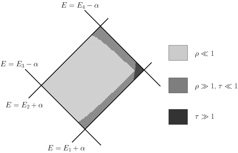
Figure 8. Comparing the coefficients $\tau$ and $\rho$ to $1$

So, for carefully chosen $\alpha$, all the phenomena described in section 1.5.1, 1.5.2 and 1.5.3, that is in figures 5, 6 and 7, do occur.

1.9. The outline of the paper

The main idea of our analysis is to reduce the spectral study of (0.1) to the study of a finite difference equation (the monodromy equation) the coefficients of which, in adiabatic limit, take a simple asymptotic form. Therefore, we use the first step of a renormalization procedure. Such renormalization procedure, called the monodromization, was first suggested to study spectral properties of the finite difference equations (on the real line) with periodic coefficients in [1]. We have understood that this idea can be generalized to study quasi periodic systems with two frequencies and, in [7], we applied it to the analysis of the differential Schrödinger equation (0.1).
In section 2, we recall the definition of the monodromy matrix and the monodromy equation for the quasi-periodic Schrödinger equation. Then, we get the asymptotic of the monodromy matrix in the adiabatic limit in the resonant case. Note that most of the technical work was already done in [3], where we have got this asymptotic in a general case; here, first, we analyze the error terms in the general formula and show that, in the resonant case, one can get for them much better estimates, second we show that, in the resonant case, one can simplify the principal term of the asymptotic.
In section 3, we prove our spectral results for the case of big $\tau$. The analysis made here is quite standard: similar calculations can be found in [5] and [3].
In section 4, we prove our results for the case of small $\tau$. This is the most complicated case. Though that we roughly follow the analysis preformed in [7] and [3], we have to develop some new ideas to be able carry out rather delicate computations. This is due to two facts: first, in the case of small $\tau$, one observes a rich set of new spectral phenomena, and, second, one has to control simultaneously several objects having different orders of exponential smallness in $\varepsilon$.
In section 1.5.3, we analyze the results of the previous section and describe the possible spectral scenarios for small $\tau$.
The main goal of section 6 is to study $\Lambda_{n}(V)$, the quantity responsible for the gap between the two resonant intervals containing spectrum. In, particular, we show that, generically, it satisfies (1.25).

2. The monodromy matrix

In this section, we first recall the definitions of the monodromy matrix and of the monodromy equation for the quasi-periodic differential equation

(2.1) $$-\frac{d^{2}}{dx^{2}}\psi(x)+(V(x-z)+\alpha\cos(\varepsilon x))\psi(x)=E\psi(x),\quad x\in{\mathbb{R}},$$

and recall how these objects related to the spectral theory of the operator $H_{z,\varepsilon}$ defined in (0.1). In the second part of the section, we describe a monodromy matrix for (2.1) in the resonant case.

2.1. The monodromy matrices and the monodromy equation

We now follow [6, 7], where the reader can find more details, results and their proofs.

2.1.1. The definition of the monodromy matrix

For any $z$ fixed, let $(\psi_{j}(x,\,z))_{j\in\{1,2\}}$ be two linearly independent solutions of equation (2.1). We say that they form a consistent basis if their Wronskian is independent of $z$, and, if for $j\in\{1,2\}$ and all $x$ and $z$,

(2.2) $$\psi_{j}(x,\,z+1)=\psi_{j}(x,\,z).$$

As $(\psi_{j}(x,\,z))_{j\in\{1,2\}}$ are solutions to equation (2.1), so are the functions $((x,z)\mapsto\psi_{j}(x+2\pi/\varepsilon,z+2\pi/\varepsilon))_{j\in\{1,2\}}$. Therefore, one can write

(2.3) $$\Psi\,(x+2\pi/\varepsilon,z+2\pi/\varepsilon)=M\,(z,E)\,\Psi\,(x,z),\quad\Psi(x,z)=\begin{pmatrix}\psi_{1}(x,\,z)\\ \psi_{2}(x,z)\end{pmatrix},$$

where $M\,(z,E)$ is a $2\times 2$ matrix with coefficients independent of $x$. The matrix $M(z,E)$ is called the monodromy matrix corresponding to the basis $(\psi_{j})_{j\in\{1,2\}}$. To simplify the notations, we often drop the $E$ dependence when not useful.

For any consistent basis, the monodromy matrix satisfies

(2.4) $$\det M\,(z)\equiv 1,\quad M\,(z+1)=M\,(z),\quad\forall z.$$

2.1.2. The monodromy equation and the link with the spectral theory of $H_{z,\varepsilon}$

Set

(2.5) $$h=\frac{2\pi}{\varepsilon}\,{\rm mod}\,1.$$

Let $M$ be the monodromy matrix corresponding to the consistent basis $(\psi_{j})_{j=1,2}$. Consider the monodromy equation

(2.6) $$F(n+1)=M\,(z+nh)F(n),\quad\quad F(n)\in{\mathbb{C}}^{2},\quad\forall n\in{\mathbb{Z}}.$$

The spectral properties of $H_{z,\varepsilon}$ defined in (0.1) are tightly related to the behavior of solutions of (2.6). This follows from the fact that the behavior of solutions of the monodromy equation for $n\to\pm\infty$ mimics the behavior of solutions of equation (0.1) for $x\to\mp\infty$, see Theorem 3.1 from [7].

2.1.3. Relations between the equations family (0.1) and the monodromy equation

Here, we describe only two consequences from Theorem 3.1 from [7]; more examples will be given in the course of the paper. One has

Theorem 2.1.

Fix $E\in{\mathbb{R}}$. Let $h$ be defined by (2.5). Let $z\mapsto M(z,E)$ be a monodromy matrix for equation (2.1) corresponding to a basis of consistent solutions that are locally bounded in $(x,z)$ together with their derivatives in $x$.
Suppose that the monodromy equation has two linearly independent solutions $(\chi_{+},\chi_{-})$ such that, for some $C>0$, for $n\in{\mathbb{N}}$, one has $\|\chi_{+}(n)\|+\|\chi_{-}(-n)\|\leq Ce^{-n/C}$. Then, $E$ belongs to the resolvent set of the operator $H_{z,\varepsilon}$.

The proof of this theorem mimics the proof of Lemma 4.1 in [7].
The second result we now present is the relation between the Lyapunov exponents of the family of equations (0.1) and of the monodromy equation.

Recall the definition of the Lyapunov exponent for a matrix cocycle. Let $z\mapsto M(z)$ be an $SL({\mathbb{C}},\,2)$-valued $1$-periodic function of the real variable $z$. Let $h$ be a positive irrational number. The Lyapunov exponent for the matrix cocycle $(M,h)$ is the limit (when it exists)

(2.7) $$\theta(M,h)=\lim_{L\to+\infty}\frac{1}{L}\log\|M(z+Lh)\cdot M(z+(L-1)h)\cdots M(z+h)\cdot M(z)\|.$$

Actually, if $M$ is sufficiently regular in $z$ (say, belongs to $L^{\infty}$), then $\theta(M,h)$ exists for almost every $z$ and does not depend on $z$, see e.g. [18].
One has

Theorem 2.2 ([6]).

Let $h$ be defined by (2.5). Let $z\mapsto M(z,E)$ be a monodromy matrix for equation (2.1) corresponding to a basis of consistent solutions that are locally bounded in $(x,z)$ together with their derivatives in $x$.  The Lyapunov exponents $\Theta(E,\varepsilon)$ and $\theta(M(\cdot,E),h)$ satisfy the relation

(2.8) $$\Theta(E,h)=\frac{\varepsilon}{2\pi}\theta(M(\cdot,E),h).$$

2.2. Asymptotics of the monodromy matrix

Consider the sequences $(E_{0}^{(l)})_{l}$ and $(E_{\pi}^{(l^{\prime})})_{l^{\prime}}$ defined by the quantization conditions (1.13). Let $E_{\pi}$ be one of the points $(E_{\pi}^{(l^{\prime})})_{l^{\prime}}$, and let $E_{0}$ be the point from the sequence $(E_{0}^{(l)})_{l}$ closest to $E_{\pi}$. Define

(2.9) $$\bar{E}=\frac{E_{0}+E_{\pi}}{2}\quad\text{and}\quad\Delta=\frac{E_{0}-E_{\pi}}{2}.$$

We assume that $E_{0}$ and $E_{\pi}$ are resonant, i.e., that they satisfy

(2.10) $$|\Delta|\leq 2e^{-\frac{\delta_{0}}{\varepsilon}}.$$

We now describe the asymptotic of the monodromy matrix for the family of equations (0.1) for (complex) energies $E$ such that

(2.11) $$|E-\bar{E}|\leq 4e^{-\frac{\delta_{0}}{\varepsilon}},\quad$$

We shall use the following notations:

1. the letter $C$ denotes various positive constants independent of $z$, $E$, $E_{\pi}$, $E_{0}$ and $\varepsilon$;

2. the symbol $O(f_{1},f_{2},\dots f_{n})$ denotes functions satisfying the estimate $|O(f_{1},f_{2},\dots f_{n})|\leq C(|f_{1}|+|f_{2}|+\dots|f_{n}|)$.

3. when writing $f\asymp g$, we mean that there exists $C>1$ such that $C^{-1}|g|\leq|f|\leq C|g|$ for all $\varepsilon$, $\zeta$, $E$, $E_{\pi}$, $E_{0}$ in consideration.

4. when writing $f=o(g)$, we mean that there exists $\varepsilon\mapsto c(\varepsilon)$, a function such that

   • $|f|\leq c(\varepsilon)|g|$ for all $\varepsilon$, $\zeta$, $E$, $E_{\pi}$ and $E_{0}$ in consideration;

   • $c(\varepsilon)\to 0$ when $\varepsilon\to 0$.

We let

(2.12) $$p(z)=e^{2\pi|{\rm Im}\,z|}.$$

Recall that $\delta_{0}$ is the constant defined in (1.11). One has

Theorem 2.3.

Pick $E_{*}\in J$. There exists $V_{*}$, a neighborhood of $E_{*}$, such that, for sufficiently small $\varepsilon$, there exists a consistent basis of solutions of (2.1) for which the monodromy matrix $(z,E)\mapsto M^{\pi}(z,E)$ is analytic in the domain $\left\{z\in{\mathbb{C}};\,2\pi|{\rm Im}\,z|<\frac{\delta_{0}}{\varepsilon}\right\}\times V_{*}^{\varepsilon}$ where $V_{*}^{\varepsilon}=\{E\in V_{*};\ |{\rm Im}\,E|\leq\varepsilon\}$. Its coefficients take real values for real $E$ and $z$. Fix $J_{*}\subset V_{*}\cap{\mathbb{R}}$, a compact interval. If $E_{\pi}\in J_{*}$ and satisfies (2.10), then, in the domain

(2.13) $$\left\{z\in{\mathbb{C}};\,2\pi|{\rm Im}\,z|<\frac{\delta_{0}}{\varepsilon}\right\}\times\left\{E\in{\mathbb{C}};\,|E-E_{\pi}|<4e^{-\frac{\delta_{0}}{\varepsilon}}\right\},$$

one has

(2.14) $$M^{\pi}=\sigma\begin{pmatrix}\tau^{2}g_{0}g_{\pi}+\bar{\theta}^{-1}&r\tau g_{0}\\ \frac{\bar{\theta}\tau}{r}g_{\pi}&\bar{\theta}\end{pmatrix}+e^{-\frac{\delta}{\varepsilon}}\,\begin{pmatrix}O\left(\tau^{2}|g|_{0}|g|_{\pi},p\right)&O\left(r\tau\,|g|_{0},p\right)\\ O\left(\frac{\tau}{r}|g|_{\pi}p,\,\bar{T}_{h}p\right)&O\left(p\right)\end{pmatrix}.$$

where $0<\delta<\delta_{0}$ is a constant depending only on $J$, $\sigma$ is constant in $\{+1,-1\}$, and, for $\nu\in\{0,\pi\}$, one has

(2.15) $$g_{\nu}(z,E)=\xi_{\nu}(E)+\sin(2\pi(z-z_{\nu})),\quad|g|_{\nu}=|\xi_{\nu}|+p,$$

(2.16) $$\xi_{\nu}(E)=\gamma_{\nu}\cdot(E-E_{\nu}).$$

Furthermore, $\tau$, $r$, $\gamma_{\nu}$, $\bar{\theta}$ and $z_{\nu}$ are real constants (independent of $z$ and $E$), one has

(2.17) $$\tau=2\sqrt{\frac{\bar{T}_{v,0}\,\bar{T}_{v,\pi}}{\bar{T}_{h}}},\quad r=\frac{\tau}{\bar{T}_{v,\pi}},$$

(2.18) $$\gamma_{\nu}=\frac{\check{\Phi}^{\prime}_{\nu}(\bar{E})}{\varepsilon\cdot\bar{T}_{v,\nu}},$$

(2.19) $$\bar{\theta}=\theta_{n}(V)(1+o(1)),$$

where $\theta_{n}(V)$ is the positive constant depending only on $n$ and $V$ defined in (6.4). and

(2.20) $$\bar{T}_{h}=t_{h}(\bar{E})\,(1+o(1)),\quad\bar{T}_{v,0}=t_{v,0}(\bar{E})\,(1+o(1)),\quad\bar{T}_{v,\pi}=t_{v,\pi}(\bar{E})\,(1+o(1)),$$

We prove this theorem in section 2.3.

Remark 2.1.

We shall also need a more detailed description of the error terms for the coefficient $M_{11}^{\pi}$. The proof of Theorem 2.3 (see the part of the proof in section 2.3.2 also yields

(2.21) $$M_{11}^{\pi}=\sigma\tau^{2}g_{0}g_{\pi}+\bar{\theta}^{-1}+e^{-\delta/\varepsilon}\,\left(\tau^{2}\left[O(\xi_{0}\xi_{\pi})+O(\xi_{0}p)+O(\xi_{\pi}p)+O(p^{2})\right]+O(p)\right),$$

where all the error terms are analytic in $E$ and in $z$.

Remark 2.2.

Being a consequence of Theorem 2.2 of[3], Theorem 2.3 stays valid if one swaps the indexes $0$ and $\pi$, and the quantities $\theta$ and $1/\theta$. One thus obtains $M^{0}$, a different monodromy matrix. Though that all the spectral results we have announced can be obtained directly by analyzing the monodromy equation with the matrix $M^{\pi}$ from Theorem 2.3, to simplify the analysis, we use from time to time the monodromy matrix $M^{0}$ instead of $M^{\pi}$.

Remark 2.3.

The notation $\tau$ (resp. $\xi_{\nu}$) in sections  ‣ 0. Introduction and 1 and the notation $\tau$ (resp. $\xi_{\nu}$) in the rest of the paper denote different quantities. They differ by a constant factor of the form $1+o(1)$ (when $\varepsilon\to 0$)!

Let us mention a case when, preserving good error estimates, one can get a more symmetric monodromy matrix:

Corollary 2.1.

In the case of Theorem 2.3, assume that $\displaystyle\tau^{2}\geq\min_{\nu\in\{0,\pi\}}\{\bar{T}_{v,\nu}\}$. Then, there exists a consistent basis of solutions of (2.1) for which the monodromy matrix $(z,E)\mapsto\tilde{M}^{\pi}(z,E)$ is analytic in the domain $\left\{z\in{\mathbb{C}};\,|{\rm Im}\,z|<\frac{\delta_{0}}{\varepsilon}\right\}\times V_{*}^{\varepsilon}$; its coefficients take real values for real $E$ and $z$. Fix $K\subset V_{*}\cap{\mathbb{R}}$ compact. If $E_{\pi}$ belongs to $K$ and satisfies (2.10), then, in the domain (2.13), one has

(2.22) $$\tilde{M}^{\pi}=\sigma\begin{pmatrix}\tau^{2}g_{0}g_{\pi}+\bar{\theta}^{-1}&\tau g_{0}\\ \bar{\theta}\tau g_{\pi}&\bar{\theta}\end{pmatrix}+e^{-\frac{\delta}{\varepsilon}}\,\begin{pmatrix}O(\tau^{2}|g|_{0}|g|_{\pi},\,p)&O(\tau|g|_{0})\\ O(p\tau|g|_{\pi})&O(p)\end{pmatrix}.$$

Remark 2.4.

The principal term in (1.33) is obtained from (2.22) by replacing $\tau$, $\bar{\theta}$ and $g_{\nu}$ (more precisely, the quantity $\xi_{\nu}$ from the definition of $g_{\nu}$) by the principal terms of their asymptotics (see also Remark 2.3).

Proof.  Let $(f_{1},f_{2})$ be the consistent basis for which the monodromy matrix is given by Theorem 2.3. Then $r^{-1/2}f_{1}$ and $r^{1/2}f_{2}$ form a consistent basis; the corresponding monodromy matrix is

$$\tilde{M}^{\pi}=\begin{pmatrix}r^{-1/2}&0\\ 0&r^{1/2}\end{pmatrix}M^{\pi}\begin{pmatrix}r^{1/2}&0\\ 0&r^{-1/2}\end{pmatrix}.$$

The asymptotic representation (2.22) follows from (2.14) and the observations that

$$r^{-1}p(z)=\frac{\bar{T}_{v,\pi}}{\tau}\,p(z)\leq\tau|g|_{0},\quad\quad\text{and}\quad\quad r\bar{T}_{h}p(z)=\frac{4r\bar{T}_{v,0}\bar{T}_{v,\pi}}{\tau^{2}}p(z)=\frac{4\bar{T}_{v,0}}{\tau}p(z)\leq 4\tau|g|_{\pi}.$$

Thus, Corollary 2.1 is proved.∎

2.3. Proof of Theorem 2.3

The matrix $M^{\pi}$ is introduced in section 3.3 in [3] ($M^{\pi}$ was denoted by $M^{U}$); there, its asymptotics are described in Theorem 3.1. Under the hypothesis (2.10) and (2.11), we improve the estimates of the error terms in the asymptotic of the coefficient $M^{\pi}_{12}$ and simplify the leading terms of the asymptotics of all the coefficients of $M^{\pi}$. This will give (2.14).
We shall use the following notations. For $(z_{1},\cdots,z_{n})\mapsto g(z_{1},\cdots,z_{n})$, an analytic function, we define

(2.23) $$g^{*}(z_{1},\cdots,z_{n})=\overline{g(\overline{z_{1}},\cdots,\overline{z_{n}})}.$$

For $Y>0$, we let

(2.24) $$T_{Y}=e^{-2\pi Y/\varepsilon}.$$

2.3.1. General asymptotic representation for the monodromy matrix $M^{\pi}$

Here, we give the asymptotics of $M^{U}$ valid without the hypotheses (2.10) and (2.11). We check

Proposition 2.1.

Pick $E_{*}\in J$. There exists $V_{*}$, a complex neighborhood of $E_{*}$, such that, for sufficiently small $\varepsilon$, the following holds. Let in (2.22),

(2.25) $$Y_{m}=\frac{1}{2\pi}\inf_{E\in J\cap V_{*}}\min(S_{0,\nu}(E),S_{\pi,\nu}(E)),\quad\quad Y_{M}=\frac{1}{2\pi}\sup_{E\in J\cap V_{*}}\max(S_{v,0}(E),S_{v,\pi}(E),S_{h}(E)).$$

Fix $0<y<Y_{m}$. There exist $Y>Y_{M}$ and a consistent basis of solutions of (2.1) for which the monodromy matrix $(z,E)\mapsto M^{U}(z,E)$ is analytic in the domain $\left\{z\in{\mathbb{C}}:\,|{\rm Im}\,z|<\frac{y}{\varepsilon}\right\}\times V_{*}^{\varepsilon}$. Its coefficients are real analytic. One has

(2.26) $$M^{\pi}(z,E)=P(z,E)+Q(z,E)+R(z,E),$$

where

(2.27) $$P(z,E)=\frac{4}{T_{h}}\,\begin{pmatrix}\tilde{C}_{\pi}(z,E)\,C_{0}(z,E)&-\tilde{S}_{\pi}(z,E)C_{0}(z,E)\\ 0&0\end{pmatrix},$$

(2.28) $$Q(z,E)=\begin{pmatrix}\frac{1}{\theta}\,\cos\frac{\check{\Phi}_{\pi}-\check{\Phi}_{0}}{\varepsilon}\,+\theta\,\cos\frac{\check{\Phi}_{\pi}}{\varepsilon}\,\cos\frac{\check{\Phi}_{0}}{\varepsilon}&-\frac{1}{\theta}\,\sin\frac{\check{\Phi}_{\pi}-\check{\Phi}_{0}}{\varepsilon}-\theta\,\sin\frac{\check{\Phi}_{\pi}}{\varepsilon}\,\cos\frac{\check{\Phi}_{0}}{\varepsilon}\\ -\theta\sin\frac{\check{\Phi}_{0}}{\varepsilon}\,\tilde{C}_{\pi}(z)&\theta\,\sin\frac{\check{\Phi}_{\pi}}{\varepsilon}\,\sin\frac{\check{\Phi}_{0}}{\varepsilon}\end{pmatrix},$$

and

(2.29) $$R_{11}(z),\ R_{12}(z),\ R_{22}(z)\ =\ O\left(T_{h},\,p(z)T_{Y}T_{h}^{-1},\,p(z)T_{v}\right),$$

(2.30) $$\begin{split}R_{21}(z)&=\cos\frac{\check{\Phi}_{\pi}}{\varepsilon}\,O\left(T_{h},\,p(z)T_{Y}T_{h}^{-1},p(z)T_{v}\right)+\cos\frac{\check{\Phi}_{0}}{\varepsilon}\,O\left(T_{h}\right)\\ &\hskip 170.71652pt+O\left(pT_{Y},\,pT_{v}T_{h},\,T_{h}^{2},\,p^{2}T_{v}T_{v,\pi},\,p^{2}T_{v,\pi}T_{Y}T_{h}^{-1}\right).\end{split}$$

In these formulae,

(2.31) $$\tilde{C}_{\pi}=\frac{\tilde{\alpha}_{\pi}e^{i\check{\Phi}_{\pi}/\varepsilon}+\tilde{\alpha}_{\pi}^{*}e^{-i\check{\Phi}_{\pi}/\varepsilon}}{2},\quad\tilde{S}_{\pi}=\frac{\tilde{\alpha}_{\pi}e^{i\check{\Phi}_{\pi}/\varepsilon}-\tilde{\alpha}_{\pi}^{*}e^{-i\check{\Phi}_{\pi}/\varepsilon}}{2i},$$

(2.32) $$C_{0}=\frac{\alpha_{0}e^{i\check{\Phi}_{0}/\varepsilon}+\alpha_{0}^{*}e^{-i\check{\Phi}_{0}/\varepsilon}}{2}.$$

The functions $(z,E)\mapsto\alpha_{0}(z,E)$ and $(z,E)\mapsto\tilde{\alpha}_{\pi}(z,E)$ are analytic in $\left\{z\in{\mathbb{C}}:\,|{\rm Im}\,z|<\frac{y}{\varepsilon}\right\}\times V_{*}^{\varepsilon}$; they are $1$-periodic in $z$ and admit the asymptotics

(2.33) $$\alpha_{0}(z,\theta)=1+T_{v,0}e^{2\pi i(z-z_{0}(E))}+O\left(T_{Y}\,p(z)\right)=1+O\left(T_{v,0}\,p(z)\right)=1+o(1),$$

(2.34) $$\begin{split}\tilde{\alpha}_{\pi}(z,\theta)=&1+T_{v,\pi}\,\left[\cos(2\pi(z-z_{\pi}))+i\sin(2\pi(z-h-z_{\pi}))\right]+O(p^{2}(z)T_{v,\pi}^{2},\,p(z)T_{Y})\\ =&1+O\left(T_{v,\pi}\,p(z)\right)=1+o(1).\end{split}$$

The functions $E\mapsto\check{\Phi}_{\nu}(E)$, $E\mapsto T_{v,\nu}(E)$, $E\mapsto z_{\nu}(E)$ and $E\mapsto T_{h}(E)$, $E\mapsto\theta(E)$ are real analytic in $V_{*}$; they are independent of $z$. In $V_{*}$, one has

(2.35) $$\check{\Phi}_{\nu}(E)=\Phi_{\nu}(E)+o(\varepsilon),$$

(2.36) $$T_{h}(E)=t_{h}(E)(1+o(1)),\quad T_{v,\nu}(E)=t_{v,\nu}(E)\,(1+o(1)),$$

where $\Phi_{\nu}$ and $t_{h}$, $t_{v,\nu}$ are the phase integrals and the tunneling coefficients defined in the introduction;

(2.37) $$\theta(E)=\theta_{n}(V)\,(1+o(1)),$$

where $\theta_{n}(V)$ is the constant defined in (6.4) (it is positive and depends only on $n$ and $V$);

(2.38) $$z_{\nu}^{\prime}(E)=O(1/\varepsilon).$$

In all the above formulae, all the error terms are analytic in $E$ and $z$. Finally, in the error term estimates, $T_{v}(E)=\max\{T_{v,0}(E),\,T_{v,\pi}(E)\}$.

Remark 2.5.

Proposition 2.1 stays valid if one swaps the indexes $0$, $\pi$, and the quantities $\theta$, $1/\theta$.

Proposition 2.1 differs from Theorem 3.1 from [3] by more precise estimate of the coefficient $R_{21}$, and, an additional information provided by Theorem 2.2, formula (2.26) and Lemma 3.4 in [3]. So, to prove Proposition 2.1, we have only to check the estimate for $R_{12}$.

Proof of the estimate for $R_{21}$.  We now analyze the structure of the term $R_{21}$ in detail. Therefore, recall the description of the matrix $M^{\pi}$ given in section 3.2 of [3] (it was denoted by $M^{U}$). It has the form

(2.39) $$M^{\pi}(z)=U(z+h)\,\begin{pmatrix}A_{\pi}(z)&B_{\pi}(z)\\ B^{*}_{\pi}(z)&A^{*}_{\pi}(z)\end{pmatrix}\,U(z)^{-1},\quad U(z)=U(z)=\frac{1}{2}\begin{pmatrix}1&1\\ -i&i\end{pmatrix}\,\begin{pmatrix}\gamma(z)&0\\ 0&\gamma^{*}(z)\end{pmatrix},$$

where $\gamma(z+h)=\sqrt{{\textstyle\frac{\alpha_{\pi}^{*}(z)}{\alpha_{\pi}(z)}}}\,e^{-i\check{\Phi}_{\pi}/\varepsilon}$. Here and below, we often drop the dependence on $E$.
The function $(z,E)\mapsto\alpha_{\pi}(z,E)$ is analytic in $\left\{z\in{\mathbb{C}}:\,|{\rm Im}\,z|<\frac{y}{\varepsilon}\right\}\times V_{*}^{\varepsilon}$; it is $1$-periodic in $z$ and admits the asymptotic representations (see Theorem 2.2 and formula (2.26) in [3])

(2.40) $$\alpha_{\pi}=1+T_{v,\pi}e^{2\pi i(z-z_{\pi})}+O\left(T_{Y}\,p(z)\right)=1+O(p(z)T_{v,\pi})=1+o(1).$$

The branch of the square root in the definition of $\gamma$ is chosen so that $\gamma(z)=e^{-i\check{\Phi}_{\pi}/\varepsilon}(1+o(1))$.
The coefficients $A_{\pi}$ and $B_{\pi}$ are described by the formulae

(2.41) $$A_{\pi}=2\,\frac{\alpha_{\pi}e^{i\frac{\check{\Phi}_{\pi}}{\varepsilon}}\,C_{0}}{T_{h}}+\alpha_{\pi}\,\alpha_{0}^{*}\,e^{i\frac{\check{\Phi}_{\pi}-\check{\Phi}_{0}}{\varepsilon}}\,\left\{\frac{\theta+1/\theta}{2}+\frac{T_{h}}{4}+\frac{O_{\pi}+O_{0}^{*}}{T_{h}}+\frac{O_{\pi}/\theta+O_{0}^{*}\theta}{2}+\frac{O_{\pi}O_{0}^{*}}{T_{h}}\right\},$$

and

(2.42) $$B_{\pi}=2\,\frac{\alpha_{\pi}e^{i\frac{\check{\Phi}_{\pi}}{\varepsilon}}\,C_{0}}{T_{h}}+\alpha_{\pi}\,e^{i\frac{\check{\Phi}_{\pi}}{\varepsilon}}\,\left\{\frac{\alpha_{0}e^{i\frac{\check{\Phi}_{0}}{\varepsilon}}/\theta+\alpha_{0}^{*}e^{-i\frac{\check{\Phi}_{0}}{\varepsilon}}\theta}{2}+\frac{\alpha_{0}e^{i\frac{\check{\Phi}_{0}}{\varepsilon}}O_{0}+\alpha_{0}^{*}e^{-i\frac{\check{\Phi}_{0}}{\varepsilon}}O_{\pi}}{T_{h}}\right\}.$$

where, for $\nu\in\{0,\pi\}$, the factor $O_{\nu}$ satisfies the estimate (see formulae (5.18) and (1.10) in [3])

(2.43) $$O_{\nu}=O(T_{h}^{2},\,T_{Y}\,p(z),\,T_{h}T_{v,\nu}p(z)).$$

Note that formulae (2.41) and (2.42) are respectively the formula (5.52) and, up to a constant factor, the formula (5.53) in [3]. The constant factor is omitted as it can be removed by conjugation (see the explanations in the last lines of section 5.3.2 in [3]).
Finally, we recall that the functions $\alpha_{\pi}$ and $\tilde{\alpha}_{\pi}$ are related by the formula

(2.44) $$\tilde{\alpha}_{\pi}(z)={\textstyle\frac{\gamma(z+h)}{\gamma(z)}}\,\alpha_{\pi}(z)$$

which is formula (3.16) in [3].
Now, we are ready to prove the estimate (2.30) for $R_{21}$. For an analytic function $f$, we let $\Im(f)=\frac{f-f^{*}}{2i}$. Representation (2.39) implies that

$$M^{\pi}_{21}=\Im(D),\quad\text{where}\quad D=\frac{\gamma(z+h)}{\gamma(z)}\,\left[A_{\pi}(z)-e^{\frac{2i\check{\Phi}_{\pi}}{\varepsilon}}\frac{\alpha_{\pi}(z)}{\alpha_{\pi}^{*}(z)}B^{*}_{\pi}(z)\right].$$

Substituting representations (2.41) and (2.42) into this formulae, we get

$$M^{\pi}_{21}=c_{0}+c_{1}+c_{2}+c_{3}+c_{4},$$

where

$$c_{0}=-\theta\,\tilde{C}_{\pi}\,\Im\left(\alpha_{0}e^{\frac{i\check{\Phi}_{0}}{\varepsilon}}\right),\quad c_{1}=\frac{T_{h}}{4}\,\Im\left(\tilde{\alpha}_{\pi}\alpha_{0}^{*}e^{\frac{i(\check{\Phi}_{\pi}-\check{\Phi}_{0})}{\varepsilon}}\right),\quad c_{2}=-\frac{2\tilde{C}_{\pi}}{T_{h}}\,\Im\left(\alpha_{0}e^{\frac{i\check{\Phi}_{0}}{\varepsilon}}O_{\pi}^{*}\right),$$

$$c_{3}=\frac{1}{2}\Im\left(\alpha_{0}^{*}\tilde{\alpha}_{\pi}e^{\frac{i(\check{\Phi}_{\pi}-\check{\Phi}_{0})}{\varepsilon}}(O_{\pi}/\theta+O_{0}^{*}\theta)\right),\quad\quad c_{4}=\frac{1}{T_{h}}\Im\left(\alpha_{0}^{*}\tilde{\alpha}_{\pi}e^{\frac{i(\check{\Phi}_{\pi}-\check{\Phi}_{0})}{\varepsilon}}O_{\pi}O_{0}^{*}\right).$$

Using the representations (2.33) and (2.34) for $\alpha_{0}$ and $\tilde{\alpha}_{\pi}$, we get

$$c_{0}=-\theta\sin\frac{\check{\Phi}_{0}}{\varepsilon}\,\tilde{C}_{\pi}+\cos\frac{\check{\Phi}_{\pi}}{\varepsilon}\,O(pT_{v,0})+O(p^{2}T_{v,0}T_{v,\pi}),$$

$$c_{1}=\sin\frac{\check{\Phi}_{\pi}-\check{\Phi}_{0}}{\varepsilon}\,T_{h}/4+O(pT_{v}T_{h},p^{2}T_{v}^{2}T_{h})=\cos\frac{\check{\Phi}_{\pi}}{\varepsilon}\,O(T_{h})+\cos\frac{\check{\Phi}_{0}}{\varepsilon}\,O(T_{h})+O(pT_{v}T_{h}),$$

where, in the last step, we have also used that $O(pT_{v})=o(1)$ for $|{\rm Im}\,\zeta|\leq y<Y_{m}$. In view of the estimate (2.43) for $O_{\pi}$, we get also

$$c_{2}=\cos\frac{\check{\Phi}_{\pi}}{\varepsilon}\,O\left(T_{h},\,pT_{Y}/T_{h},\,pT_{v,\pi}\right)+O\left(pT_{v,\pi}T_{h},\,p^{2}T_{v,\pi}T_{Y}/T_{h},\,p^{2}T_{v,\pi}^{2}\right).$$

Finally, as $|\alpha_{0}|+|\tilde{\alpha}_{\pi}|=O(1)$, in view of (2.43) and as $|{\rm Im}\,z|\leq y<Y_{M}<Y$, we get

$$c_{3}=O\left(T_{h}^{2},\,pT_{Y},\,pT_{v}T_{h}\right),\quad c_{4}=O\left(T_{h}^{3},p^{2}T_{Y}^{2}/T_{h},p^{2}T_{v}^{2}T_{h}\right).$$

These estimates imply the announced representation for $M^{\pi}_{21}$, and complete the proof of the estimate for $R_{21}$. ∎

2.3.2. Asymptotics of the monodromy matrix in the resonant case

We now simplify the asymptotics for the coefficients of the monodromy matrix given by Proposition 2.1 in the resonant case.
In this section, $J_{*}$ always denotes a compact interval in $V_{*}\cap J$.
For $\nu\in\{0,\pi\}$, we let

(2.45) $$\sigma_{\nu}=-\sin\frac{\check{\Phi}_{\nu}(E_{\nu})}{\varepsilon},\quad\text{and}\quad\sigma=\sigma_{0}\sigma_{\pi}.$$

Note that, by the definition of $E_{\nu}$, one has $\sigma_{\nu}\in\{+1,-1\}$, and $\sigma\in\{+1,-1\}$.
Define

(2.46) $$\bar{T}_{v,\nu}=T_{v,\nu}(\bar{E}),\quad\bar{T}_{h}=T_{h}(\bar{E}),\quad\text{and}\quad\bar{\theta}=\theta(\bar{E}).$$

Clearly, these quantities satisfy (2.20) and (2.19).
First, for later use, we recall

Lemma 2.1 ([3], Lemma 2.1).

There exists a neighborhood of $J_{*}$, say $\tilde{V}_{*}$, and $C>0$ such that, for sufficiently small $\varepsilon$, for $E\in\tilde{V}_{*}$ and $\nu\in\{0,\pi\}$, one has

$$|\check{\Phi}_{\nu}^{\prime}(E)|+|\check{\Phi}_{\nu}^{\prime\prime}(E)|\leq C,\quad{\rm and}\quad\frac{1}{C}\leq|\check{\Phi}_{\nu}^{\prime}(E)|.$$

Now, we check two simple lemmas.

Lemma 2.2.

Pick $\nu\in\{0,\pi\}$. Fix $C>0$. For $\varepsilon$ sufficiently small, if $E_{\nu}\in J_{*}$ and $|E-E_{\nu}|\leq Ce^{-\delta_{0}/\varepsilon}$, one has

(2.47) $$\cos\frac{\check{\Phi}_{\nu}(E)}{\varepsilon}=\sigma_{\nu}\frac{\check{\Phi}_{\nu}^{\prime}(\bar{E})}{\varepsilon}\cdot(E-E_{\nu})\left(1+O\left(\varepsilon^{-1}e^{-\delta_{0}/\varepsilon}\right)\right)$$

(2.48) $$\sin\frac{\check{\Phi}_{\nu}(E)}{\varepsilon}=-\sigma_{\nu}+O\left(\varepsilon^{-2}e^{-2\delta_{0}/\varepsilon}\right).$$

Proof.  Both estimates follow from Lemma 2.1 and the definition of $E_{\nu}$. We note only that to get (2.48) one uses (2.47). This completes the proof of Lemma 2.2. ∎
Estimate (2.47) implies that

(2.49) $$\cos\frac{\check{\Phi}_{\nu}(E)}{\varepsilon}=\sigma_{\nu}\bar{T}_{v,\nu}\xi_{\nu}\left(1+O\left(\varepsilon^{-1}e^{-\delta_{0}/\varepsilon}\right)\right),\quad\text{and}\quad\left|\cos\frac{\check{\Phi}_{\nu}(E)}{\varepsilon}\right|\leq C\varepsilon^{-1}e^{-\delta_{0}/\varepsilon},$$

where $\xi_{\nu}$ are the local variables defined in (2.16).
We now prove

Lemma 2.3.

Let $\bar{E}\in J_{*}$. For $\varepsilon$ sufficiently small, for $E$ satisfying (2.11), one has

$$T_{h}(E)=\bar{T}_{h}\,(1+O(\varepsilon^{-1}e^{-\frac{\delta_{0}}{\varepsilon}})),\quad T_{v,0}(E)=\bar{T}_{v,0}\,(1+O(\varepsilon^{-1}e^{-\frac{\delta_{0}}{\varepsilon}})),\quad T_{v,\pi}(E)=\bar{T}_{v,\pi}\,(1+O(\varepsilon^{-1}e^{-\frac{\delta_{0}}{\varepsilon}}),$$

$$\theta=\bar{\theta}\,(1+O(e^{-\frac{\delta_{0}}{\varepsilon}})),\quad\quad z_{\nu}(E)=z_{\nu}(\bar{E})+O(\varepsilon^{-1}e^{-\frac{\delta_{0}}{\varepsilon}})$$

Proof.  Prove the representation for $T_{h}$. Recall that, in $V_{*}$, a neighborhood of $E_{*}$ independent of $\varepsilon$,  $T_{h}$ admits the asymptotics from (2.35). This and the Cauchy estimates for the derivatives of analytic functions imply that, for $E$ in any fixed compact of $V_{*}$, one has $|\frac{d}{dE}\log T_{h}|\leq C\varepsilon^{-1}$. So, for $E$ satisfying (2.11), we get $T_{h}(E)=\bar{T}_{h}(1+O(\varepsilon^{-1}e^{-\delta_{0}/\varepsilon})$. The estimates for $T_{v,0}$ and $T_{v,\pi}$ are proved similarly.
Furthermore, (2.37) implies that, for $E$ in any fixed compact of $V_{*}$, one has $|\theta^{\prime}(E)|\leq C$. This implies the asymptotic representation for $\bar{\theta}$. The asymptotic representation for $z_{\nu}$ follows from (2.38) in the same way. This completes the proof of Lemma 2.3. ∎
We now derive simplified asymptotic representations for the functions $\tilde{C}_{\pi}$, $\tilde{S}_{\pi}$ and $C_{0}$ defined in (2.31) and (2.32). Redefine $z_{0}:=z_{0}(\bar{E})$, and $z_{\pi}:=z_{\pi}(\bar{E})-2\pi h$. We prove

Lemma 2.4.

Let $E_{\pi}\in J_{*}$, let (2.10) hold. For $\varepsilon$ sufficiently small, for all $(z,E)$ in the domain (2.13), one has

(2.50) $$\begin{split}C_{0}&=\sigma_{0}\bar{T}_{v,0}g_{0}+\varepsilon^{-1}e^{-\delta_{0}/\varepsilon}\bar{T}_{v,0}\,O\left(\xi_{0},p\right)+O\left(T_{Y}p\right),\\ \tilde{C}_{\pi}&=\sigma_{\pi}\bar{T}_{v,\pi}g_{\pi}+\varepsilon^{-1}e^{-\delta_{0}/\varepsilon}\bar{T}_{v,\pi}O\left(\xi_{\pi},p\right)+O\left(T_{Y}p\right),\quad\quad\tilde{S}_{\pi}=-\sigma_{\pi}+O\left(e^{-\delta_{0}/\varepsilon}\right).\end{split}$$

Proof.  Prove (2.50). From (2.32) and (2.33), we get

$$C_{0}=\cos\frac{\check{\Phi}_{0}(E)}{\varepsilon}+T_{v,0}\cos\left(2\pi(z-z_{0})+\frac{\check{\Phi}_{0}(E)}{\varepsilon}\right)+O(pT_{Y})$$

with the “old” $z_{0}$. By means of Lemmas 2.2,and 2.3, this yields

$$C_{0}=\sigma_{0}\bar{T}_{v,0}(\xi_{0}+\sin(2\pi(z-z_{0}))+\varepsilon^{-1}e^{-\delta_{0}/\varepsilon}\bar{T}_{v,0}\,O(\xi_{0},p)+O(T_{Y}p)$$

already with the “new” $z_{0}$. This result and (2.15) imply (2.50).
The asymptotic representations for $\tilde{C}_{\pi}$ and $\tilde{S}_{\pi}$ are proved similarly; we only note that one uses the estimate $p\bar{T}_{v,\nu}\leq e^{-\delta_{0}/\varepsilon}$ which follows from the definitions of $p$ and $\delta_{0}$ (as $2\pi|{\rm Im}\,z|\leq\delta_{0}/\varepsilon$). This completes the proof of Lemma 2.4.∎
Now, we are ready to derive Theorem 2.3 from Proposition 2.1. Begin by computing $M^{\pi}_{11}$ for $E$ and $E_{\pi}\in J_{*}$ satisfying (2.11) and (2.10). By (2.26), we have

(2.51) $$M^{\pi}_{11}=P_{11}+Q_{11}+R_{11}.$$

By (2.27) and Lemmas 2.4 and 2.3, for sufficiently small $\varepsilon$, we get

$$\begin{split}P_{11}=&\sigma_{0}\sigma_{\pi}\,\frac{4}{\bar{T}_{h}}\,\left(1+O(\varepsilon^{-1}e^{-\delta_{0}/\varepsilon})\right)\cdot\\ &\left(\bar{T}_{v,0}g_{0}+\varepsilon^{-1}e^{-\delta_{0}/\varepsilon}\bar{T}_{v,0}O\left(\xi_{0},p\right)+\,\,O\left(T_{Y}p\right)\right)\,\left(\bar{T}_{v,\pi}g_{\pi}+\varepsilon^{-1}e^{-\delta_{0}/\varepsilon}\bar{T}_{v,\pi}O\left(\xi_{\pi},p\right)+O\left(T_{Y}p\right)\right).\end{split}$$

Now, recalling the definitions of $\tau$ and $g_{\nu}$, see (2.17) and (2.15), we get

$$P_{11}=\sigma_{0}\sigma_{\pi}\,\tau^{2}g_{0}g_{\pi}+\tau^{2}\varepsilon^{-1}e^{-\delta_{0}/\varepsilon}O\left(\xi_{0}\xi_{\pi},p\xi_{0},p\xi_{\pi},p^{2}\right)+O\left(p\frac{T_{Y}}{\bar{T}_{h}}\left(e^{-\delta_{0}/\varepsilon}/\varepsilon+(\bar{T}_{v,\pi}+\bar{T}_{v,0})p+T_{Y}p\right)\right)$$

Note that, by (1.11), for $2\pi|{\rm Im}\,z|\leq\delta_{0}/\varepsilon$, one has

(2.52) $$(\bar{T}_{h}+\bar{T}_{v,0}+\bar{T}_{v,\pi})p\leq Ce^{-2\delta_{0}/\varepsilon}p\leq Ce^{-\delta_{0}/\varepsilon}.$$

Recall that $Y>Y_{M}$ (see Theorem 2.1) and note that $T_{h}\geq e^{-2\pi Y_{M}/\varepsilon}$, see (2.25). Let $\delta_{1}=2\pi(Y-Y_{M})$. Then,

(2.53) $$T_{Y}/\bar{T}_{h}\leq Ce^{-\delta_{1}/\varepsilon}.$$

Therefore, we get

(2.54) $$P_{11}=\sigma_{0}\sigma_{\pi}\,\tau^{2}g_{0}g_{\pi}+\tau^{2}\varepsilon^{-1}e^{-\delta_{0}/\varepsilon}O\left(\xi_{0}\xi_{\pi},p\xi_{0},p\xi_{\pi},p^{2}\right)+O\left(pe^{-(\delta_{1}+\delta_{0})/\varepsilon}\right).$$

Furthermore, by (2.28) and Lemmas 2.2 and 2.3, we have

$$Q_{11}=\theta^{-1}\,\cos\frac{\check{\Phi}_{\pi}-\check{\Phi}_{0}}{\varepsilon}\,+\theta\,\cos\frac{\check{\Phi}_{\pi}}{\varepsilon}\,\cos\frac{\check{\Phi}_{0}}{\varepsilon}=\bar{\theta}^{-1}\sigma_{\pi}\sigma_{0}+O(e^{-\delta_{0}/\varepsilon}).$$

Finally, by (2.29) and estimates (2.52) and (2.53), we get

$$R_{11}=O\left(T_{h},\,p(z)T_{Y}T_{h}^{-1},\,p(z)T_{v}\right)=O(pe^{-\delta_{1}/\varepsilon},e^{-\delta_{0}/\varepsilon}).$$

Fix $0<\delta<\min(\delta_{0},\delta_{1})$. Substituting the estimates obtained for $P_{11}$, $Q_{11}$ and $R_{11}$ into (2.51), and using the notation $\sigma=\sigma_{0}\sigma_{\pi}$, we get the representation for $M_{11}^{\pi}$ announced in Theorem 2.3. The representations for the other coefficients of the matrix $M^{\pi}$ are proved with the same technique.
We only briefly comment on how to derive the representation for $M_{21}^{U}$. By (2.26) and (2.27), one has

$$M_{21}^{U}=Q_{21}+R_{21}.$$

First, one shows that

$$Q_{21}=\sigma\bar{\theta}\tau g_{\pi}/r+\varepsilon^{-1}e^{-\delta_{0}/\varepsilon}\,\tau r^{-1}\,O(\xi_{\pi},p)+O(e^{-\delta_{1}/\varepsilon}T_{h}p).$$

The representation for $M_{21}^{U}$ follows from the one for $Q_{21}$ and the estimate

$$R_{21}=e^{-\delta/\varepsilon}\,\tau r^{-1}\,O(p\xi_{\pi},p^{2})+e^{-\delta/\varepsilon}\,O(\bar{T}_{h}p)$$

which follows from (2.30) and the estimates

$$\cos\frac{\check{\Phi}_{\pi}}{\varepsilon}\,O\left(T_{h},\,p(z)T_{v}\right)=e^{-\delta_{0}/\varepsilon}\tau r^{-1}O(\xi_{\pi}),\quad\cos\frac{\check{\Phi}_{\pi}}{\varepsilon}\,O\left(pT_{Y}/T_{h}\right)=e^{-\delta_{1}/\varepsilon}\tau r^{-1}O(p\xi_{\pi}),$$

$$\cos\frac{\check{\Phi}_{0}}{\varepsilon}\,O\left(T_{h}\right)=\varepsilon^{-1}e^{-\delta_{0}/\varepsilon}O(\bar{T}_{h}),\quad\quad O\left(p^{2}T_{v}T_{v,\pi}\right)=e^{-\delta_{0}/\varepsilon}\tau r^{-1}O(p),$$

$$O\left(p^{2}\frac{T_{v,\pi}T_{Y}}{T_{h}}\right)=e^{-\delta_{1}/\varepsilon}\tau r^{-1}O\left(p^{2}\right),\quad\quad O\left(pT_{Y},\,pT_{v}T_{h},\,T_{h}^{2}\right)=e^{-\delta/\varepsilon}O(p\bar{T}_{h}).$$

We omit further details of the proof of Theorem 2.3. ∎

3. The case of large $\tau$

In this section, we prove Theorem 1.2. We fix $E_{*}\in J$, assume that $\varepsilon$ is so small that Theorem 1.1 holds, and systematically use notations from this theorem.
In this section, we work under the condition $\tau\gg 1$; by (1.20), this means that, for some $\delta_{\tau}>0$,

(3.1) $$\tau\geq e^{\delta_{\tau}/\varepsilon}.$$

Let $\bar{V}=\{E\in{\mathbb{C}}:\ |E-\bar{E}|\leq 4e^{-\delta_{0}/\varepsilon}\}$. Here, we study the spectrum of $H_{z,\varepsilon}$ in $R=\bar{V}\cap{\mathbb{R}}$.
As $\tau\gg 1$, we shall use the monodromy matrix $\tilde{M}$ described by Corollary 2.1.

3.0.1. Intervals containing spectrum

Fix $N>0$. For each $\nu\in\{0,\pi\}$, we let

$$I_{\nu}(N)=\{E\in J;\ |\xi_{\nu}(E)|\leq 1+\varepsilon^{N}\}.$$

We prove

Theorem 3.1.

For sufficiently small $\varepsilon$, the spectrum of $H_{z,\varepsilon}$ in $R$ is contained in $I_{0}(N)\cup I_{\pi}(N)$.

The proof of this theorem is based upon

Proposition 3.1 ([1], Proposition 3.1).

Fix $E\in{\mathbb{R}}$ and define $h$ by (2.5). Let $z\mapsto M(z,E)$ be a monodromy matrix for equation (2.1) corresponding to a basis of consistent solutions that are locally bounded in $(x,z)$ together with their derivatives in $x$.
Define

(3.2) $$\rho(z)=M_{12}(z)/M_{12}(z-h),\quad v(z)=M_{11}(z)+\rho(z)\,M_{22}(z).$$

Suppose that

(3.3) $$\min_{z\in{\mathbb{R}}}|M_{12}(z)|>0,\quad\max_{z\in{\mathbb{R}}}|\rho(z)|<\left(\frac{1}{2}\,\min_{z\in{\mathbb{R}}}|v(z)|\right)^{2},\quad\text{ind}\,\rho=\text{ind}\,v=0,$$

where $\text{ind}\,g$ is the index of a continuous periodic function $g$.

Then, $E$ is in the resolvent set of (0.1).

Note that the proof of this proposition is based on Theorem 2.1.
Proof of Theorem 3.1.  It suffices to prove that, for $\varepsilon$ small enough, for $E$ in $R\setminus(I_{0}(N)\cup I_{\pi}(N))$, the monodromy matrix $\tilde{M}$ described in Corollary 2.1 satisfy the assumptions of Proposition 3.1.
Below, we always assume that $z\in{\mathbb{R}}$.
1.  In terms of the coefficients of $\tilde{M}^{\pi}$ (see Corollary 2.1), define the function $\rho$ by (3.2). We prove that, for sufficiently small $\varepsilon$, for $E\in R\setminus I_{0}(N)$ and $z\in{\mathbb{R}}$, one has

(3.4) $$|\tilde{M}^{\pi}_{12}|>0,\quad{\rm and}\quad|\rho|\leq C\varepsilon^{-N}.$$

By Corollary 2.1, we have

(3.5) $$\tilde{M}^{\pi}_{12}=\sigma\tau g_{0}(1+e^{-\delta/\varepsilon}O(|g|_{0}/g_{0})).$$

By (2.15), for $E\in R\setminus I_{0}(N)$, one has

(3.6) $$|g_{0}|\geq\varepsilon^{N},\quad 1\leq\left|\frac{|g|_{0}}{g_{0}}\right|\leq\frac{|\xi_{0}|+1}{||\xi_{0}|-1|}\leq\varepsilon^{-N}(2+\varepsilon^{N}),\quad\left|\frac{g_{0}(z)}{g_{0}(z-h)}\right|\leq\varepsilon^{-N}(1+\varepsilon^{N}).$$

For $\varepsilon$ sufficiently small, (3.5) and (3.6) imply (3.4).
2.  Here, we assume that $E\in R\setminus(I_{0}(N)\cup I_{\pi}(N))$. In terms of the coefficients of $\tilde{M}^{\pi}$, define the function $v$ by (3.2). Check that

(3.7) $$v=\sigma\tau^{2}g_{0}g_{\pi}(1+o(1))\quad\text{and}\quad|v|\geq C\varepsilon^{2N}e^{2\delta_{\tau}/\varepsilon}.$$

We have

(3.8) $$|g_{0}g_{\pi}|\geq(|\xi_{0}|-1)(|\xi_{\pi}|-1)\geq\varepsilon^{2N}\quad\text{and}\quad\frac{|g|_{0}|g|_{\pi}}{|g_{0}g_{\pi}|}\leq\frac{(|\xi_{0}|+1)(|\xi_{\pi}|+1)}{(|\xi_{0}|-1)(|\xi_{\pi}|-1)}\leq\varepsilon^{-2N}(2+\varepsilon^{N})^{2}.$$

Using the asymptotics of $\tilde{M}^{\pi}$ given by (2.22), estimates (3.8) and (3.4), we get

$$v=\sigma\tau^{2}g_{0}g_{\pi}+\bar{\theta}^{-1}+e^{-\frac{\delta}{\varepsilon}}\,O(\tau^{2}|g|_{0}|g|_{\pi},\,1)+\rho(z)(\bar{\theta}+O(e^{-\frac{\delta}{\varepsilon}}))=\sigma\tau^{2}g_{0}g_{\pi}(1+O(\varepsilon^{-2N}e^{-\frac{\delta}{\varepsilon}},\,\varepsilon^{-3N}\tau^{-2})).$$

In view of (3.1), this implies the first estimate in (3.7). The latter, (3.1) and the first estimate from (3.8) imply the second estimate in (3.7).
3.  Steps 1 and 2 imply that, for sufficiently small $\varepsilon$ and $E\in R\setminus(I_{0}(N)\cup I_{\pi}(N))$, the matrix $\tilde{M}$ satisfies the conditions of Proposition 3.1 (note that the equalities $\text{ind}\,v=\text{ind}\,\rho=0$ follow from the inequalities $|v|,\,|\tilde{M}^{\pi}_{12}|>0$ and the fact that the coefficients of the monodromy matrix $\tilde{M}^{\pi}$ are real valued). This implies the statement of Theorem 3.1.∎
One has

Corollary 3.1.

Fix $N>0$. For sufficiently small $\varepsilon$, the interval $I_{0}(N)$ (resp. $I_{\pi}(N)$) is contained in the $(C\varepsilon t_{v,0}(\bar{E}))$-neighborhood (resp. $(C\varepsilon\bar{t}_{v,\pi}(\bar{E}))$-neighborhood) of the point $E_{0}$ (resp $E_{\pi}$).

Proof.  The result follows from Theorem 3.1, the definitions of $I_{\nu}(N)$, the definitions of $\xi_{\nu}$, see (2.16) and (2.18), Lemma 2.1 and (2.20).∎
We shall also use a rougher result

Corollary 3.2.

For sufficiently small $\varepsilon$, in the case of Theorem 3.1, $I_{0}(N)$ (resp. $I_{\pi}(N)$) is contained in the $(C\varepsilon e^{-2\delta_{0}/\varepsilon})$-neighborhood of the point $E_{0}$ (resp. $E_{\pi}$).

Proof.  This follows from the previous statement as, for each $\nu\in\{0,\pi\}$, one has $t_{v,\nu}(\bar{E})\leq e^{-2\delta_{0}/\varepsilon}$. ∎

3.1. Computation of the integrated density of states

We now compute the increment of the integrated density of states on the intervals $I_{0}$ and $I_{\pi}$ described in the previous subsection. We prove

Theorem 3.2.

Fix $N>0$. For sufficiently small $\varepsilon$,

(3.9) $$\int_{I_{0}(N)\cup I_{\pi}(N)}n_{\varepsilon}(dE)=\frac{\varepsilon}{\pi},\quad{\rm and}\quad\int_{I_{0}(N)}n_{\varepsilon}(dE)=\int_{\check{I}_{\pi}}n_{\varepsilon}(dE)=\frac{\varepsilon}{2\pi}\ \text{if}\ I_{0}(N)\cap I_{\pi}(N)=\emptyset,$$

where $n_{\varepsilon}(dE)$ denotes the density of states measure of $H_{z,\varepsilon}$.

Proof. The proof of this theorem is based upon

Proposition 3.2 ([3], Proposition 4.2).

Pick two points $a<b$ of the real axis. Let $\gamma$ be a continuous curve in ${\mathbb{C}}_{+}$ connecting $a$ and $b$.
Assume that, for all $E\in\gamma$, there is a consistent basis such that the following holds.

• The basis solutions are locally bounded in $(x,z)$ together with their first derivatives in $x$.

• There exists $V(\gamma)$, a neighborhood of $\gamma$ such that the monodromy matrix is continuous in $(z,E)\in{\mathbb{R}}\times V(\gamma)$ and analytic in $E\in V(\gamma)$.

• On $\gamma$, the coefficients of $M$, the monodromy matrix, satisfy the conditions (3.3) in which $\rho$ and $v$ are defined by (3.2) with $h$ from (2.5).

• the coefficients of $M$ are real for real $E$ and $z$.

Then, the increment of the integrated density of states on the interval $[a,b]$ is given by

(3.10) $$\int_{a}^{b}n_{\varepsilon}(dE)=-\left.\frac{\varepsilon}{2\pi^{2}}\int_{0}^{1}\arg v(z,E)\,dz\right|_{\gamma},$$

where $f|_{\gamma}$ denotes the increment of $f$ when going from $a$ to $b$ along $\gamma$.

The proof of Theorem 3.2 consists of the following steps.
1. First, we assume that $I_{0}(N)\cap I_{\pi}(N)=\emptyset$ and prove that $\int_{I_{0}(N)}n_{\varepsilon}(dE)=\varepsilon/2\pi$.
By (1.22), $\xi_{0}$ is a non constant affine function of $E$. To apply Proposition 3.2, as $\gamma$ we choose the half circle

$$\gamma=\{E\in{\mathbb{C}}:\ |\xi_{0}(E)|=1+\varepsilon^{N+1},\,{\rm Im}\,E\geq 0\}.$$

Recall that $a<b$ denote the ends of $\gamma$. Now, $[a,b]=I_{0}(N)$. So, $I_{0}(N+2)\subset]a,b[$, and $[a,b]\cap I_{\pi}(N)=\emptyset$. So, by Theorem 3.1, $a$ and $b$ are in the resolvent set of $H_{z,\varepsilon}$.
Note also that, for sufficiently small $\varepsilon$, for $E\in\gamma$, one has

(3.11) $$|E-\bar{E}|\leq 2e^{-\delta_{0}/\varepsilon}.$$

Indeed, by (2.10), one has $|E_{0}-\bar{E}|\leq e^{-\delta_{0}/\varepsilon}$, and, for sufficiently small $\varepsilon$, for $E\in\gamma$, we get

$$|E-E_{0}|=\varepsilon\bar{T}_{v,0}|\check{\Phi}_{0}^{\prime}(\bar{E})|^{-1}\,\,|\xi_{0}(E)|\leq C\varepsilon t_{v,0}(\bar{E})\leq C\varepsilon e^{-2\delta_{0}/\varepsilon},$$

where we have used the definitions of $\xi_{0}$, of $\gamma$, Lemma 2.1, (2.20) and the definitions of $\delta_{0}$ and $t_{v,0}$.
By (3.11), $(z,E)\in{\mathbb{R}}\times\gamma$ is in the domain (2.13), so, we can use the matrix $\tilde{M}^{\pi}$ from Corollary 2.1 and its asymptotics (2.22). Define $\rho$ and $v$ in terms of $\tilde{M}^{\pi}$ by (3.2). To apply the Proposition 3.2, we need only to check that, along $\gamma$, condition (3.3) is satisfied. This follows from the

Lemma 3.1.

For sufficiently small $\varepsilon$, for $E\in\gamma$ and $z\in{\mathbb{R}}$, one has

(3.12) $$\begin{split}\tilde{M}^{\pi}_{12}&\neq 0,\quad\quad\text{ind}\,\rho=0,\quad\quad|\rho|\leq C\varepsilon^{-N-1},\\ v&=\sigma\tau^{2}g_{0}g_{\pi}(1+o(1)),\quad\quad\text{ind}\,v=0,\quad\quad|v|\geq C\varepsilon^{2(N+1)}e^{2\delta_{\tau}/\varepsilon}.\end{split}$$

Proof.  When proving this lemma, one uses almost the same arguments as in the proof of Theorem 3.1 with $N$ replaced by $N+1$. The only difference is that now one deduces the equalities $\text{ind}\,\rho=\text{ind}\,v=0$ from the asymptotic $\tilde{M}^{\pi}_{12}=\sigma\tau g_{0}(1+o(1)$ and the asymptotics of $v$ from (3.12). We omit further details.∎
As the integrated density of states is constant outside the spectrum, formula (3.10) and the representation for $v$ in (3.12) give

$$\frac{2\pi^{2}}{\varepsilon}\int_{I_{0}(N)}n_{\varepsilon}(dE)=-\left.\int_{0}^{1}\arg v(z,E)\,dz\right|_{\gamma}=-\left.\int_{0}^{1}\arg(g_{0}g_{\pi})dz\right|_{\gamma}.$$

where, in the last step, we have used the fact that, for $z$ and $E$ real, the functions $v$, $g_{0}$ and $g_{\pi}$ take real values, and, therefore, the last two integrals coinciding up to $o(1)$, they are equal. As, for $E\in\gamma$, one has $|g_{\nu}/\xi_{\nu}-1|<1$, $\nu\in\{0,\pi\}$, and as $\xi_{\nu}$ and $g_{\nu}$ are real for real $z$ and $E$, we get finally

$$\int_{I_{0}(N)}n_{\varepsilon}(dE)=-\frac{\varepsilon}{2\pi^{2}}\left.\int_{0}^{1}\arg(\xi_{0}\xi_{\pi})dz\right|_{\gamma}=-\left.\frac{\varepsilon}{2\pi^{2}}\cdot\arg((E-E_{0})(E-E_{\pi}))\right|_{\gamma}=\frac{\varepsilon}{2\pi},$$

where we have used the fact that only $E_{0}$ is located between the ends of $\gamma$ and $E_{\pi}$ is not.
2.  Now, to complete the proof of Theorem 3.2, it suffices to check the first equality in (3.9). Therefore, we use the same techniques as in the previous step. So, we only outline the proof.
Now, we take

$$\gamma=\{E\in{\mathbb{C}}:\ |E-\bar{E}|=2e^{-\delta_{0}/\varepsilon},\,{\rm Im}\,E\geq 0\}.$$

Now, both $E_{0}$ and $E_{\pi}$ are between the ends of $\gamma$. Moreover, by Corollary 3.2, both $E_{0}$ and $E_{\pi}$ are between the ends of $\gamma$. Define $\rho$ and $v$ in terms of $\tilde{M}^{\pi}$ by (3.2). One proves

Lemma 3.2.

For sufficiently small $\varepsilon$, for $E\in\gamma$ and $z\in{\mathbb{R}}$, one has

$$\tilde{M}^{\pi}_{12}\neq 0,\quad\rho=1+o(1),\quad\text{ind}\,\rho=0,\quad\quad v=\sigma\tau^{2}\xi_{0}\xi_{\pi}(1+o(1)),\quad\text{ind}\,v=0,\quad|\tau^{2}\xi_{0}\xi_{\pi}|\geq C/\varepsilon^{2}.$$

Proof.  One uses essentially the same analysis as when proving Theorem 3.1 and Lemma 3.1. We omit the details, noting only that, now, for sufficiently small $\varepsilon$, for each $\nu\in\{0,\pi\}$ and $E\in\gamma$,

$$|\xi_{\nu}(E)|\geq C\varepsilon^{-1}t_{v,\nu}^{-1}(\bar{E})|E-E_{\nu}|\geq C\varepsilon^{-1}e^{2\delta_{0}/\varepsilon}(|E-\bar{E}|-|\bar{E}-E_{\nu}|)\geq C\varepsilon^{-1}e^{\delta_{0}/\varepsilon}.\quad\quad\text{ \qed}$$

This lemma immediately implies that the conditions of Proposition 3.2 are satisfied. The points $E_{0}$ and $E_{\pi}$ being between the ends of $\gamma$, one obtains

$$\int_{I_{0}(N)\cup I_{\pi}(N)}n_{\varepsilon}(dE)=-\left.\frac{\varepsilon}{2\pi^{2}}\cdot\arg((E-E_{0})(E-E_{\pi}))\right|_{\gamma}=\frac{\varepsilon}{\pi}.$$

This completes the proof of (1.23).

3.2. Computation of the Lyapunov exponent

Here, we compute the asymptotics of the Lyapunov exponent $\Theta(E,\varepsilon)$ on the intervals $I_{0}(N)$ and $I_{\pi}(N)$ and prove

Theorem 3.3.

Fix $N>0$. For sufficiently small $\varepsilon$, for $E\in I_{0}(N)\cup I_{\pi}(N)$, one has (1.24).

To compute $\Theta(E,\varepsilon)$, we use Theorem 2.2 and the matrix cocycle $(\tilde{M}^{\pi},h)$. In the next two subsections, we get an upper and a lower bound for $\theta(\tilde{M}^{\pi},h)$. They will coincide up to smaller order terms, and, thus, lead to the asymptotic formula for $\Theta(E,\varepsilon)$.
In sections 3.2.1, 3.2.2 and 3.2.3, we always assume that $E\in I_{0}(N)\cup I_{\pi}(N)$.

3.2.1. The upper bound

We now prove that

(3.13) $$\theta(\tilde{M}^{\pi},h)\leq 2\log\left(\tau\sqrt{1+|\xi_{0}(E)|+|\xi_{\pi}(E)|}\right)+C.$$

Therefore, we first note that (2.22) implies that

$$\|M^{\pi}(z,E)\|\leq C\tau^{2}(|\xi_{0}|+1)(|\xi_{\pi}|+1),\quad z\in{\mathbb{R}}.$$

Note that to get this estimate, we have used that $\tau>1$.
As $E\in(I_{0}(N)\cup I_{\pi}(N))$, then, by Theorem 3.1, for sufficiently small $\varepsilon$, at least one of the inequalities

$$|\xi_{0}|\leq 2,\quad\text{and}\quad|\xi_{\pi}|\leq 2.$$

is satisfied. Therefore, we get

$$\|M^{\pi}(z,E)\|\leq C\tau^{2}(|\xi_{0}|+|\xi_{\pi}|+1),\quad z\in{\mathbb{R}}.$$

Now, this estimate and the definition of Lyapunov exponent for matrix cocycles (2.7) imply (3.13).

3.2.2. The lower bound for the Lyapunov exponent

Here, we prove that

(3.14) $$\theta(\tilde{M}^{\pi},h)\geq 2\log\left(\tau\sqrt{1+|\xi_{0}(E)|+|\xi_{\pi}(E)|}\right)+O(1).$$

Therefore, we use the following construction.
Assume that a matrix function $M:{\mathbb{C}}\to SL(2,{\mathbb{C}})$ is $1$-periodic and depends on a parameter $\varepsilon>0$. One has

Proposition 3.3.

Pick $\varepsilon_{0}>0$. Assume that there exist $y_{0}$ and $y_{1}$ satisfying the inequalities $0<y_{0}<y_{1}<\infty$ and such that, for any $\varepsilon\in(0,\varepsilon_{0})$ one has

• the function $z\to M(z,\varepsilon)$ is analytic in the strip $S=\{z\in{\mathbb{C}};\ 0\leq{\rm Im}\,z\leq y_{1}/\varepsilon\}$;

• in the strip $S=\{z\in{\mathbb{C}};\ y_{0}/\varepsilon\leq{\rm Im}\,z\leq y_{1}/\varepsilon\}\subset S$, $M(z,\varepsilon)$ admits the following uniform in $S$ representation

  (3.15) $$M(z,\varepsilon)=\lambda(\varepsilon)e^{2\pi imz}\cdot\left(\begin{pmatrix}1&0\\ 0&0\end{pmatrix}+o(1)\right),\quad\varepsilon\to 0,$$

  where $\lambda(\varepsilon)$ and $m$ are independent of $z$, and $m$ is an integer independent of $\varepsilon$.

Then, there exists $\varepsilon_{1}>0$ such that, if $0<\varepsilon<\varepsilon_{1}$, one has

(3.16) $$\theta(M,h)>\log|\lambda(\varepsilon)|+o(1);$$

the number $\varepsilon_{1}$ and the error estimate in (3.16) depend only on $\varepsilon_{0}$, $y_{0}$, $y_{1}$ and the norm of the term $o(1)$ in (3.15).

This proposition immediately follows from Proposition 10.1 from [7]. Note that the proof of the latter is based on the ideas of [21] generalizing Herman’s argument [11].

Consider the case where $E\in I_{0}(N)$. Then, one has $|\xi_{0}|<2$ (for $\varepsilon<1$). Fix $0<y_{0}<y_{1}<\frac{\delta}{2\pi}$, where $\delta$ is the constant from (2.22). We shall describe the precise choice of $y_{0}$ and $y_{1}$ later. For sufficiently small $\varepsilon$ and $\frac{y_{0}}{\varepsilon}\leq|{\rm Im}\,z|\leq\frac{y_{1}}{\varepsilon}$, representation (2.22) implies that

(3.17) $$\tilde{M}^{\pi}=\frac{\sigma\tau^{2}}{2i}\,e^{-2\pi i(z-z_{0})}\cdot\left[\begin{pmatrix}\xi_{\pi}(1+o(1))+\frac{1}{2i}e^{-2\pi i(z-z_{\pi})}(1+o(1))&0\\ \xi_{\pi}\cdot o(1)&0\end{pmatrix}+o(1)\right].$$

We have used (3.1). Now, let $y=\frac{\varepsilon}{2\pi}\log(1+|\xi_{\pi}(E)|)$. Fix $0<A<\delta/2\pi$.
To compute the Lyapunov exponent for $E\in I_{0}(N)$ such that $y\leq A$, we choose $y_{0}>A$. Then, for sufficiently small $\varepsilon$, for such $E$, we get

$$\tilde{M}^{\pi}=-\frac{\sigma\tau^{2}}{4}\,e^{-2\pi i(2z-z_{0}-z_{\pi})}\cdot\left[\begin{pmatrix}1&0\\ 0&0\end{pmatrix}+o(1)\right],$$

and so, Proposition 3.3 implies that $\theta(\tilde{M},h)\geq\log(\tau^{2}/4)+o(1)$.
On the other hand, to compute the Lyapunov exponent for all $E\in I_{0}(N)$ such that $y\geq A$, we choose $y_{1}<A$. Then, for sufficiently small $\varepsilon$, for all such $E$, we get

$$\tilde{M}^{\pi}=\frac{\sigma\tau^{2}}{2i}\,\xi_{\pi}\,e^{-2\pi i(z-z_{\nu})}\cdot\left[\begin{pmatrix}1&0\\ 0&0\end{pmatrix}+o(1)\right],$$

and so, Proposition 3.3 implies that $\theta(\tilde{M},h)\geq\log(\tau^{2}|\xi_{\pi}|/2)+o(1)$.
For sufficiently small $\varepsilon$ and for $E\in I_{0}(N)$, the obtained lower bounds for $\theta(\tilde{M}^{\pi},h)$ imply (3.14).
For $E\in I_{\pi}(N)$, one proves (3.14) similarly.

3.2.3. Completing the analysis

Theorem 2.2 and estimates (3.13) and (3.14) imply that, for sufficiently small $\varepsilon$, on $I_{0}\cup I_{\pi}$, one has (1.24). This completes the proof of Theorem 3.3.

4. The case of small $\tau$

We now turn to the case $\tau\ll 1$; by (1.21), this means that, for some $\delta_{\tau}>0$,

(4.1) $$\tau\leq e^{-\delta_{\tau}/\varepsilon}.$$

We shall assume that (1.25) holds. As before, we fix $E_{*}\in J$, assume that $\varepsilon$ is so small that Theorem 1.1 holds, and we systematically use its notations.
Let $\bar{V}=\{E\in{\mathbb{C}}:\ |E-\bar{E}|\leq 4e^{-\delta_{0}/\varepsilon}\}$ and study the spectrum in $R=\bar{V}\cap{\mathbb{R}}$. Now, we use the monodromy matrix $M^{\pi}$ described by Theorem 2.3.

4.1. The location of the spectrum

In this section, we prove Theorem 1.3. The central point of its proof is the a priori estimate provided by

Lemma 4.1.

Under the above conditions, for sufficiently small $\varepsilon$, if $E\in R\cap\sigma(H_{z,\varepsilon})$, then

(4.2) $$\tau^{2}(|\xi_{0}(E)|+1)(|\xi_{\pi}(E)|+1)\geq C(1+o(1)),$$

where $o(1)$ depends only on $\varepsilon$, and $C$ depends only on $\theta_{n}(V)$.

First, in sections 4.1.1 and 4.1.2, we prove Lemma 4.1. Then, in section 4.1.3, by means of this lemma, we get a description of the resolvent set of $H_{z,\varepsilon}$ inside $\tilde{R}=\{E\in R$ satisfying (4.2)$\}$. This will yield Theorem 1.3.

4.1.1. Proof of the a priori estimate

The proof of Lemma 4.1 is based on the following construction.
Consider the finite difference equation

(4.3) $$\psi(z+h)=M(z)\psi(z),\quad z\in{\mathbb{R}},$$

where $h$ is a fixed positive number, and $M$, a fixed matrix function in $L^{\infty}(R,SL(2,{\mathbb{C}}))$. One has

Proposition 4.1.

Suppose that, for $z\in{\mathbb{R}}$, $M(z)$ can be represented as

(4.4) $$M(z)=\begin{pmatrix}\theta^{-1}&0\\ 0&\theta\end{pmatrix}+\tilde{M}(z),$$

where $\theta$ is a real number, and this number and the matrix valued function $z\mapsto\tilde{M}(z)$ satisfy

(4.5) $$|\theta+\theta^{-1}|>2\quad\text{and}\quad|\theta-\theta^{-1}|\geq 4\sup_{1\leq i,j\leq 2}\sup_{z\in{\mathbb{R}}}|\tilde{M}_{ij}(z)|.$$

Then, there exists $\psi_{+}$ and $\psi_{-}$, two vector solutions to (4.3) in $L^{\infty}_{\rm loc}({\mathbb{R}},{\mathbb{C}}^{2})$, such that, for $z\in{\mathbb{R}}$,

(4.6) $$\det(\psi_{+}(z),\psi_{-}(z))>0\quad\text{and}\quad\|\psi_{+}(z)\|_{{\mathbb{C}}^{2}}+\|\psi_{-}(-z)\|_{{\mathbb{C}}^{2}}\leq Ce^{-z\log\frac{|\theta+\theta^{-1}|}{2}},\quad\text{if}\quad z>0.$$

Let us first derive Lemma 4.1 from Proposition 4.1 applied to $M=M^{\pi}$ and $h$ defined by (2.5). We represent $M^{\pi}$ in the form (4.4) with $\theta=\bar{\theta}$. Then, for $z\in{\mathbb{R}}$, by Theorem 2.3, one has

$$|\tilde{M}_{11}|\leq\tau^{2}(|\xi_{0}|+1)(|\xi_{\pi}|+1)(1+o(1))+O(e^{-\delta/\varepsilon}),\quad|\tilde{M}_{22}|\leq O(e^{-\delta/\varepsilon}),$$

(4.7) $$|\tilde{M}_{12}\tilde{M}_{21}|\leq\bar{\theta}\tau^{2}(|\xi_{0}|+1)(|\xi_{\pi}|+1)(1+o(1))+O(e^{-\delta/\varepsilon}).$$

Only the last estimate requires to be checked. From (2.14), for $z\in{\mathbb{R}}$, we get

$$|\tilde{M}_{12}\tilde{M}_{21}| \leq\left(r\tau(|\xi_{0}|+1)(1+o(1))+Ce^{-\delta/\varepsilon}\right)\,\left(\bar{\theta}r^{-1}\tau(|\xi_{\pi}|+1)(1+o(1))+C\bar{T}_{h}e^{-\delta/\varepsilon}\right)$$

$$\leq\bar{\theta}\tau^{2}(|\xi_{0}|+1)(|\xi_{\pi}|+1)(1+o(1))+Ce^{-\delta/\varepsilon}\left(\bar{T}_{v,0}((|\xi_{0}|+1)+\bar{T}_{v,\pi}((|\xi_{\pi}|+1)+e^{-\delta/\varepsilon}\bar{T}_{h}\right)$$

$$\leq\bar{\theta}\tau^{2}((|\xi_{0}|+1)(|\xi_{\pi}|+1)(1+o(1))$$

$$\hskip 85.35826pt+Ce^{-\delta/\varepsilon}\left(\varepsilon^{-1}\,|E-E_{0}|+\bar{T}_{v,0}+\varepsilon^{-1}\,|E-E_{\pi}|+\bar{T}_{v,\pi}+e^{-\delta/\varepsilon}\bar{T}_{h}\right)$$

which implies (4.7).
The estimates for the coefficients of the matrix $\tilde{M}$ show that $M^{\pi}$ is similar to a matrix of the form (4.4) for which

$$\sup_{1\leq i,j\leq 2}\sup_{z\in{\mathbb{R}}}|\tilde{M}_{ij}(z)|\leq\max\{a,\sqrt{\bar{\theta}a}\}\quad\text{where}\quad a=\tau^{2}((|\xi_{0}|+1)(|\xi_{\pi}|+1)(1+o(1))+Ce^{-\delta/\varepsilon}.$$

This and Proposition 4.1 imply that, if

(4.8) $$\bar{\theta}+{\bar{\theta}}^{-1}>2\quad\text{and}\quad a<C(\bar{\theta})=\min\left\{(\bar{\theta}-\bar{\theta}^{-1})/4,(\bar{\theta}-\bar{\theta}^{-1})^{2}/(16\theta)\right\},$$

then, there exist $(\psi_{+},\psi_{-})$, the two solutions to (4.3) for $M=M^{\pi}$, that have all the properties described in Proposition 4.1. Define functions $\chi_{\pm}:\ {\mathbb{Z}}\mapsto{\mathbb{C}}^{2}$ by $\chi_{\pm}(n)=\psi_{\pm}(nh+z)$. The functions $\chi_{+}$ and $\chi_{-}$ are solutions to the monodromy equation (2.6) satisfying the conditions of Theorem 2.1. So, $E$ is in the resolvent set of $H_{z,\varepsilon}$.
Finally, discuss the conditions (4.8). Fix $0<q<1$. Recall that $\bar{\theta}$ admits the asymptotics (2.37), and that $\theta_{n}(V)+\theta^{-1}_{n}(V)=2\Lambda_{n}(V)>2$. Therefore, if $\tau^{2}((|\xi_{0}|+1)(|\xi_{\pi}|+1)<qC(\bar{\theta})$, then, for sufficiently small $\varepsilon$, the conditions (4.8) are satisfied. This implies Lemma 4.1. So, to complete the proof of this result, we only have to check Proposition 4.1.

4.1.2. Proof of Proposition 4.1

Set

(4.9) $$m=\sup_{1\leq i,j\leq 2}\sup_{z\in{\mathbb{R}}}|\tilde{M}_{ij}(z)|.$$

Note that, if $\psi$ is a solution to (4.4), then $e^{\pi iz/h}\psi(z)$ satisfies the same equation with $M$ replaced by $-M$, and for $\sigma=\begin{pmatrix}0&1\\ 1&0\end{pmatrix}$, $\sigma\psi$ satisfies equation (4.4) with $M$ replaced by $\sigma M\sigma$. Therefore, it suffices to consider the case $\theta>1$. The proof then consists of five steps.
1.  We begin by the following elementary observation. Let $G$ be a solution of the equation

(4.10) $$G(z+h)=\frac{M_{11}(z)G(z)+M_{12}(z)}{M_{21}(z)G(z)+M_{22}(z)},\quad z\in{\mathbb{R}},$$

and let $\psi_{2}(z)$ be a solution of the equation

(4.11) $$\psi_{2}(z+h)=(M_{21}(z)G(z)+M_{22}(z))\psi_{2}(z),\quad z\in{\mathbb{R}}.$$

Then, the vector function defined by $\psi(z)=\psi_{2}(z)\begin{pmatrix}G(z)\\ 1\end{pmatrix}$ is a solution to (4.3). The proof of this observation being elementary, we omit it.
2.  Let

$$q=\frac{\theta-\theta^{-1}}{2m}-1-\sqrt{\left(\frac{\theta-\theta^{-1}}{2m}-1\right)^{2}-1}.$$

Recall that $\theta>1$ and satisfies conditions (4.5). One has

(4.12) $$q^{2}-2\left(\frac{\theta-\theta^{-1}}{2m}-1\right)q+1=0;$$

$$0<q<1;$$

(4.13) $$p=\theta-m(q+1)>\frac{\theta^{-1}+\theta}{2}>1.$$

The first relation is obvious; the lower bound follows from the second condition in (4.5); the upper bound follows from the facts that the second solution to (4.12) is greater than $q$ and that the product of the solutions is equal to one; (4.13) follows from the equality

$$\theta-m(q+1)=\frac{\theta^{-1}+\theta}{2}+m\sqrt{\left(\frac{\theta-\theta^{-1}}{2m}-1\right)^{2}-1}$$

and the first condition in (4.5).
3. Let us construct a bounded solution to (4.10). For $z\in{\mathbb{R}}$ and $k\geq 1$, let

(4.14) $$G_{k+1}(z+h)=\frac{M_{11}(z)G_{k}(z)+M_{12}(z)}{M_{21}(z)G_{k}(z)+M_{22}(z)},\quad\text{and}\quad G_{0}(z)=0.$$

One has

(4.15) $$\sup_{z\in{\mathbb{R}}}|G_{k+1}(z)|\leq q,\quad k\in{\mathbb{N}}^{*}.$$

Indeed, this estimate is valid for $G_{0}$. Assume that it has been proved for a positive integer $k$; using (4.14) and (4.12), we get

$$\sup_{z\in{\mathbb{R}}}|G_{k+1}(z)|\leq\frac{(\theta^{-1}+m)q+m}{\theta-m-mq}=q.$$

Now, check prove that $\{G_{k}(\cdot)\}_{k=0}^{\infty}$ converges in $L^{\infty}$. It suffices to prove that, for $k\in{\mathbb{N}}^{*}$,

(4.16) $$\sup_{z\in{\mathbb{R}}}|G_{k+1}(z)-G_{k}(z)|\leq\frac{m}{p^{2k+1}}.$$

Here, $p$ has been defined in (4.13). In view of (4.15) and (4.9), we get

$$\sup_{z\in{\mathbb{R}}}|G_{1}(z+h)-G_{0}(z+h)|\leq m/(\theta-m)<m/p;$$

and for $$k\geq 1 z\in{\mathbb{R}}$$ and

$$\begin{split}|G_{k+1}(z+h)-G_{k}(z+h)|&=\left|\frac{\det M(z-h)\cdot(G_{k}(z-h)-G_{k-1}(z-h))}{(M_{21}(z)G_{k}(z)+M_{22}(z))(M_{21}(z)G_{k-1}(z)+M_{22}(z))}\right|\\ &\leq\frac{1}{p^{2}}|G_{k}(z-h)-G_{k-1}(z-h)|.\end{split}$$

Here, we have used $\det M=1$; this is the only place in the proof of Proposition 4.1 where we use this property. The above estimates then imply (4.16).
Denote by $G$ the limit of $\{G_{k}(\cdot)\}_{k=0}^{\infty}$. Clearly, $G$ is a solution to (4.10) and satisfies $|G(z)|\leq q$.
4. Consider equation (4.11) with $G$ constructed in the previous step. To construct a solution to this equation, it suffices to define it on the interval $[0,h)$ and continue it outside this interval by induction using equation (4.3); that is, for $n\geq 1$ and $z\in[0,h)$, one sets

$$\psi_{2}(z+nh)=(M_{21}(z+(n-1)h)G(z+(n-1)h)+M_{22}(z+(n-1)h))\psi_{2}(z+(n-1)h),$$

$$\psi_{2}(z-nh)=(M_{21}(z-nh)G(z-nh)+M_{22}(z-nh))^{-1}\psi_{2}(z-(n-1)h).$$

Note that, for all $z\in{\mathbb{R}}$, one has $|M_{21}(z)G(z)+M_{22}(z)|\geq\theta-m(q+1)=p>0$, and, so, for $n\geq 1$ and $z\in[0,h)$, the second formula correctly defines $\psi_{2}$ for negative $z$.
Let $\psi_{2}(z)=1$ for $z\in[0,h)$. Then, by construction, for $z\in[-nh,-(n-1)h)$ and $n\in{\mathbb{N}}$, one has $|\psi_{2}(z)|\leq p^{-n}$. In terms of $\psi_{2}$, we construct a vector solution to (4.3) as described in step 1. We denote the thus constructed solution by $\psi_{-}$; it satisfies

$$\psi_{-}(z)=\begin{pmatrix}G(z)\\ 1\end{pmatrix}\text{ for }\ z\in[0,h)\quad\text{and}\quad\|\psi_{-}(-z)\|\leq\sqrt{1+q^{2}}e^{-\log p\cdot z/h}\leq\sqrt{1+q^{2}}e^{-\gamma z/h}\text{ for }z\geq 0,$$

where $\gamma=\log\frac{\theta+\theta^{-1}}{2}$.
5.  Construct the solution $\psi_{+}$. Therefore, consider the equation (4.3) with the matrix $\sigma M^{-1}(-z-h)\sigma$ replacing $M(z)$. The matrix $\sigma M^{-1}(-z-h)\sigma$ can be written in the form (4.4) with the old $\theta$ and the matrix $\sigma\tilde{M}^{-1}(-z-h)\sigma$ instead of $\tilde{M}(z)$. Clearly, with the matrix $M$, it satisfies all the hypotheses of Proposition 4.1. So, as when constructing $\psi_{-}$, we can construct $\tilde{\psi}_{-}$, a solution to the equation (4.3) for the matrix $\sigma M^{-1}(-z-h)\sigma$. When constructing this solution, in the last step, we normalize it by setting $\tilde{\psi}_{2}=1$ on the interval $(-h,0]$. Then, we get

$$\tilde{\psi}_{-}(z)=\begin{pmatrix}\tilde{G}(z)\\ 1\end{pmatrix}\text{ for }\ z\in[-h,0)\quad\text{and}\quad\|\tilde{\psi}_{-}(-z)\|\leq\sqrt{1+q^{2}}e^{-\gamma(z-h)/h}\text{ for }z\geq 0.$$

Here, $\tilde{G}$ is a function satisfying the estimate $|\tilde{G}(z)|\leq q$ for all $z\in{\mathbb{R}}$.
Having constructed $\tilde{\psi}_{-}$, we define $\psi_{+}:{\mathbb{R}}\mapsto{\mathbb{C}}^{2}$ by the formula $\psi_{+}(z)=\sigma\tilde{\psi}_{-}(-z)$. The function $\psi_{+}$ satisfies (4.3) for the matrix $M$, and one has

$$\psi_{+}(z)=\begin{pmatrix}1\\ \tilde{G}(-z)\end{pmatrix}\text{ for }\ z\in[0,h)\quad\text{and}\quad\|\psi_{+}(z)\|\leq e^{\gamma}\sqrt{1+q^{2}}e^{-\gamma z/h}\text{ for }z\geq 0.$$

6. To complete the proof of Proposition 4.1, we need only to check that $\det(\psi_{+},\psi_{-})\neq 0$. From equation (4.3), it follows that this determinant is $h$-periodic. So, it suffices to consider $z\in[0,h)$. Then, one has $\det(\psi_{+},\psi_{-})=1-G(z)\tilde{G}(-z)$, and so, $|\det(\psi_{+},\psi_{-})-1|=|G(z)\tilde{G}(-z)|\leq q^{2}<1$. This completes the proof of Proposition 4.1.∎

4.1.3. Completing the proof of Theorem 1.3

The proof of Theorem 1.3 consists of three steps. In the first two steps, we apply Proposition 3.1 to the monodromy equations with the matrix $M^{\pi}$ and $M^{0}$ (see Remark 2.2). When we can do it, $E$ is outside the spectrum of $H_{z,\varepsilon}$. In this case, we see that, if $E$ is in the spectrum of $H_{z,\varepsilon}$, then, it satisfies (1.26). In the third step, we analyze the case when one can not apply Proposition 3.1; using the a priori estimate from Lemma 4.1, we see that then $E$ is outside the spectrum of $H_{z,\varepsilon}$.
Below, we consider only $z\in{\mathbb{R}}$. Fix $\delta_{\xi}>0$. The precise choice of this constant will be described later using the a priori estimate (4.2).
1.  By Theorem 2.3, one has

$$M_{12}^{\pi}=\sigma r\tau(\xi_{0}+\sin(2\pi(z-z_{0}))+e^{-\frac{\delta}{\varepsilon}}\cdot O(r\tau(|\xi_{0}|+1),1).$$

Assume that $E$ satisfies

(4.17) $$\xi_{0}(E)\geq e^{\delta_{\xi}/\varepsilon}\cdot\max\{1,\,(r\tau)^{-1}e^{-\frac{\delta}{\varepsilon}}\}.$$

Then, we get

(4.18) $$M_{12}^{\pi}=\sigma\,r\,\tau\,\xi_{0}(1+o(1)).$$

So, we have $M_{12}^{\pi}\neq 0$.
In terms of the monodromy matrix $M^{\pi}$, define the functions $\rho$ and $v$ by (3.2). By means of (4.18) and Theorem 2.3, for sufficiently small $\varepsilon$, we get

(4.19) $$\rho=1+o(1),$$

(4.20) $$v=\sigma\left(\tau^{2}\left(\xi_{0}+\sin(2\pi(z-z_{0}))\right)\left(\xi_{\pi}+\sin(2\pi(z-z_{\pi}))+o(|\xi_{\pi}|+1)\right)+2\Lambda_{n}(V)\right)+o(1);$$

when deriving the representation for $v$, we have also used (2.37) and (6.4).
As the coefficients of $M^{\pi}$ are real when $E$ and $z$ are real, one has $\text{ind}\,\rho=\text{ind}\,v=0$ as soon as $|\rho|$ is bounded away from zero, and $v$ satisfy the second condition in (3.3). By (4.1), (4.19) and (4.20), there exists a function $\varepsilon\mapsto f_{0}(\varepsilon)$ that is $o(1)$ when $\varepsilon$ is small such that the first bound in (3.3) is satisfied when

(4.21) $$\left|\tau^{2}\xi_{0}\xi_{\pi}+2\Lambda_{n}(V)\right|\geq\left(2+\tau^{2}|\xi_{0}|+\tau^{2}|\xi_{\pi}|\right)\,(1+f_{0}).$$

So, for sufficiently small $\varepsilon$, if $E$ satisfies (4.21), it is outside the spectrum of $H_{z,\varepsilon}$.
2.  Now, assume that $E$ satisfies

(4.22) $$|\xi_{\pi}(E)|\geq e^{\delta_{\xi}/\varepsilon}\cdot\max\{1,\,r\tau^{-1}e^{-\frac{\delta}{\varepsilon}}\bar{T}_{h}\}.$$

In this case, for sufficiently small $\varepsilon$, there exists a function $\varepsilon\mapsto f_{\pi}(\varepsilon)$ that is $o(1)$ for $\varepsilon$ small such that, if $E$ satisfies

(4.23) $$\left|\tau^{2}\xi_{0}\xi_{\pi}+2\Lambda_{n}(V)\right|\geq\left(2+\tau^{2}|\xi_{0}|+\tau^{2}|\xi_{\pi}|\right)\,(1+f_{\pi}).$$

then $E$ is outside the spectrum of $H_{z,\varepsilon}$.
Though this result can be obtained by using directly the matrix $M_{\pi}$, the proof becomes immediate if, instead of $M^{\pi}$, one uses the matrix $M^{0}$, see Remark 2.2. Note that the conditions (4.17) and (4.22) are equivalent respectively to

$$\xi_{0}(E)\geq e^{\delta_{\xi}/\varepsilon}\cdot\max\{1,\,2e^{-\frac{\delta}{\varepsilon}}\bar{T}_{h}/\bar{T}_{v,0}\}\quad{\rm and}\quad\xi_{\pi}(E)\geq e^{\delta_{\xi}/\varepsilon}\cdot\max\{1,\,2e^{-\frac{\delta}{\varepsilon}}\bar{T}_{h}/\bar{T}_{v,\pi}\},$$

and when one swaps the indices $0$ and $\pi$, one swaps these two conditions. So, the proof of (4.23) is obtained from the one of (4.21) just by swapping the indices. This completes the second step.
3. We prove

Lemma 4.2.

Fix $\delta_{\xi}$ so that

(4.24) $$0<\delta_{\xi}<\max\{\delta_{\tau},\delta_{0}\}.$$

For sufficiently small $\varepsilon$, in the case of Theorem 1.3, all the energies $E$ that satisfy neither (4.17) nor (4.22) are outside the spectrum of $H_{z,\varepsilon}$.

Proof.  Pick $E$ that satisfies neither (4.17) nor (4.22). Then, one has

$$\tau^{2}(|\xi_{\pi}(E)|+1)(|\xi_{0}(E)| +1)\leq C\tau^{2}e^{2\delta_{\xi}/\varepsilon}\cdot\left(1+r\tau^{-1}e^{-\frac{\delta}{\varepsilon}}\bar{T}_{h}\right)\,\left(1+(r\tau)^{-1}e^{-\frac{\delta}{\varepsilon}}\right)$$

$$=Ce^{2\delta_{\xi}/\varepsilon}\cdot\left(\tau^{2}+e^{-\frac{\delta}{\varepsilon}}\left(\bar{T}_{v,\pi}+\bar{T}_{v,0}\right)+e^{-2\frac{\delta}{\varepsilon}}\bar{T}_{h}\right)\leq Ce^{2\delta_{\xi}/\varepsilon}\cdot\left(e^{-\frac{2\delta_{\tau}}{\varepsilon}}+e^{-\frac{\delta+2\delta_{0}}{\varepsilon}}\right),$$

where, in the second step, we have used (2.17), and, in the last step, we have used (2.20) and (1.11). In view of the last computation and (4.24), we get that $\tau^{2}(|\xi_{\pi}(E)|+1)(|\xi_{0}(E)|+1)=o(1)$, and, in view of Lemma 4.1, for sufficiently small $\varepsilon$, this implies, that $E$ is outside the spectrum of $H_{z,\varepsilon}$. This completes the proof of Lemma 4.2.∎
Now, let $f(\varepsilon)=\max\{f_{0}(\varepsilon),f_{\pi}(\varepsilon)\}$. Clearly, for sufficiently small $\varepsilon$, the function $f$ is well defined and satisfies $f=o(1)$ near $0$. By Lemma 4.2 and the first two steps, we see that, if $E$ in $R$ is in the spectrum of $H_{z,\varepsilon}$, then, it satisfies $\left|\tau^{2}\xi_{0}\xi_{\pi}+2\Lambda_{n}(V)\right|\leq\left(2+\tau^{2}|\xi_{0}|+\tau^{2}|\xi_{\pi}|\right)\,(1+f)$. This completes the proof of Theorem 1.3.∎

4.2. Properties of the set defined by (1.26)

We now analyze (1.26) and prove Proposition 1.1.
Let

(4.25) $$G(E)=\tau^{2}\xi_{0}(E)\xi_{\pi}(E)+2\Lambda_{n}(V),\quad\text{and}\quad F(E)=\left(2+\tau^{2}|\xi_{0}(E)|+\tau^{2}|\xi_{\pi}(E)|\right)(1+f(\varepsilon)),$$

where the function $\varepsilon\mapsto f(\varepsilon)$ is defined in Theorem 1.3. So, the condition (1.26) takes the form:

(4.26) $$|G(E)|\leq F(E).$$

4.2.1. Individual properties of $F$ and $G$

We first discuss various properties of the functions $G$ and $F$ without comparing their graphs, i.e., without analyzing (4.26).

Lemma 4.3.

One has

1. $G$ is a quadratic polynomial in $E$;

2. it reaches its maximum at $\bar{E}$;

3. $G(E_{0})=G(E_{\pi})=2\Lambda_{n}(V)>2$;

4. $F$ is affine except at the points $E_{0}$ and $E_{\pi}$;

5. $F$ is strictly increasing for $E>\max\{E_{0},E_{\pi}\}$, strictly decreasing for $E<\min\{E_{0},E_{\pi}\}$;

6. between $E_{0}$ and $E_{\pi}$, the absolute value of the derivative of $F$ is smaller than it is for $E>\max\{E_{0},E_{\pi}\}$ or $E<\min\{E_{0},E_{\pi}\}$;

7. $F(E_{\pi})=(2+\tau^{2}|\xi_{0}(E_{\pi})|)(1+f)$ and $F(E_{0})=(2+\tau^{2}|\xi_{\pi}(E_{0})|)(1+f)$.

Proof.  Lemma follow from (2.16) and (4.25). To prove point (2) one also uses (2.18) and (1.4). ∎

4.2.2. The intervals $I_{\rm in}$ and $I_{\rm out}$

Now, we begin the analysis of condition (4.26). First, we describe the set $\{E\in{\mathbb{R}};\ G(E)\geq F(E)\}$.

Corollary 4.1.

For sufficiently small $\varepsilon$, the set $I_{\rm in}=\{E\in{\mathbb{R}};\ G(E)\geq F(E)\}$ is a compact interval of positive length. It is located strictly between the zeros of the polynomial $G$.

Proof.  Lemma 4.3 implies that $G$ is concave (points (1) and (2)). As $F$ is positive, $I_{\rm in}$ (if not empty) is located between the zeros of $G$. By the points (4) – (6) of Lemma 4.3, $F$ is convex. So, now, it suffices to prove, that for sufficiently small $\varepsilon$, there exists a point $\tilde{E}$, where $G(\tilde{E})>F(\tilde{E})$. Therefore, note that $0=|\xi_{0}(E_{0})|\leq|\xi_{\pi}(E_{0})|$, and that $0=|\xi_{\pi}(E_{\pi})|\leq|\xi_{0}(E_{\pi})|$. This implies that, between $E_{0}$ and $E_{\pi}$, there is $\tilde{E}$, a point where $\xi_{0}(\tilde{E})=\xi_{\pi}(\tilde{E})$. Denote this common value by $\xi$. At $\tilde{E}$, one has

$$\begin{split}G(\tilde{E})-F(\tilde{E})&=\tau^{2}|\xi|^{2}+2\Lambda_{n}(V)-2(1+\tau^{2}|\xi|)(1+f)\\ &=\tau^{2}(|\xi|-1-f)^{2}+2(\Lambda_{n}(V)-1-f)-(1+f)^{2}\\ &\geq 2(\Lambda_{n}(V)-1-f)-\tau^{2}(1+f)^{2}.\end{split}$$

Therefore, for sufficiently small $\varepsilon$, one has $G(\tilde{E})-F(\tilde{E})>\Lambda_{n}(V)-1>0$. This completes the proof of Corollary 4.1.∎
We now prove

Corollary 4.2.

The set $I_{\rm out}=\{E\in{\mathbb{R}};\ G(E)\geq-F(E)\}$ is a compact interval of positive length. Moreover, $I_{\rm in}$ is contained in $\dot{I}_{\rm out}$, the interior of $I_{\rm out}$.

Proof.  Let $\varepsilon$ be so small that $I_{\rm in}$ exists and that $F>0$ for all $E\in{\mathbb{R}}$. On the compact interval bounded by $E_{\pi}$ and $E_{0}$, the function $G$ is positive (see points (2) and (3) of Lemma 4.3), whereas $-F$ is negative. This, the facts that $G$ is a concave quadratic polynomial and $-F$ is piecewise affine and concave (by Lemma 4.3) imply that $I_{\rm out}$ is a compact interval of positive length. The inclusion $I_{\rm in}\subset\dot{I}_{\rm out}$ follows from the inequality $G(E)\geq F(E)>-F(E)$ valid for $E\in I_{\rm in}$.∎

4.2.3. The intervals $I_{\rm l}$ and $I_{\rm r}$

Let $\Sigma(\varepsilon)$ be the set where condition (4.26) is satisfied. One has $\Sigma(\varepsilon)=I_{\rm out}\setminus\dot{I}_{\rm in}$. Corollaries 4.1 and 4.2 imply

Corollary 4.3.

For sufficiently small $\varepsilon$, the set $\Sigma(\varepsilon)$ consists of two disjoint compact intervals of positive length.

We denote these intervals by $I_{\rm l}$ and $I_{\rm r}$ so that $I_{\rm l}$ be to the left of $I_{\rm r}$. We finally check

Lemma 4.4.

For $\varepsilon$ sufficiently small, both $I_{l}$ and $I_{r}$ are inside the $(2e^{-\delta_{0}/\varepsilon})$-neighborhood of $\bar{E}$.

Proof.  It suffices to check that outside the $(2e^{-\delta_{0}/\varepsilon})$-neighborhood of $\bar{E}$, one has $|G(E)|\geq F(E)$. By (1.11) and Lemma 2.1, for $E$ such that $|E-\bar{E}|\geq 2e^{-\delta_{0}/\varepsilon}$ and $\nu\in\{0,\pi\}$, one has

$$|\xi_{\nu}(E)|=\frac{|\check{\Phi}_{\nu}^{\prime}(\bar{E})(E-E_{\nu})|}{\varepsilon\bar{T}_{v,\nu}}\,\geq\frac{e^{\frac{\delta_{0}}{\varepsilon}}}{C\varepsilon},\quad\tau^{2}|\xi_{0}(E)\xi_{\pi}(E)|=\frac{4|\check{\Phi}_{0}^{\prime}(\bar{E})\check{\Phi}_{\pi}^{\prime}(\bar{E})(E-E_{0})(E-E_{\pi})|}{\varepsilon^{2}\bar{T}_{h}}\geq\frac{1}{C\varepsilon^{2}}.$$

For sufficiently small $\varepsilon$, these estimates imply that, for $|E-\bar{E}|\geq 2e^{-\delta_{0}/\varepsilon}$ and $\nu\in\{0,\pi\}$,

$$|G(E)|-F(E)\geq\tau^{2}(|\xi_{0}(E)|-1-f)(|\xi_{\pi}(E)|-1-f)-2(\Lambda_{n}(V)-1-f)-\tau^{2}(1+f)^{2}\geq\frac{1}{C\varepsilon^{2}}.$$

This completes the proof of Lemma 4.4.∎

Corollary 4.3 and Lemma 4.4 prove Proposition 1.1.

4.3. Computing the density of states

We now compute the increments of the integrated density of states on each of the intervals defined in Proposition 1.1 and, thus, prove Theorem 1.4.
We assume that

(4.27) $$\bar{T}_{v,\pi}\geq\bar{T}_{v,0}.$$

The complementary case is treated similarly, but instead of working with $M^{\pi}$, one uses the monodromy matrix $M^{0}$ mentioned in Remark 2.2. For sake of definiteness, we assume that $\sigma=1$ in (2.14) and that

(4.28) $$E_{\pi}\leq E_{0}.$$

The cases where $E_{\pi}\geq E_{0}$ or $\sigma=-1$ are analyzed similarly.
Our main tool is Proposition 3.2. First, we compute the increment of the integrated density of states on the whole set $\Sigma_{\varepsilon}$ and, then, we compute it on one of the intervals of this set.

4.3.1. The increment of the IDS on the set $\Sigma_{\varepsilon}$

As the curve used to apply Theorem 3.2, we choose

(4.29) $$\gamma=\{E\in{\mathbb{C}};\ |E-\bar{E}|=2\,e^{-\delta_{0}/\varepsilon},\ {\rm Im}\,E\geq 0\}.$$

Lemma 4.4 implies that the set $\Sigma_{\varepsilon}$ is strictly between the ends of $\gamma$.
The analysis of the increment of the integrated density of states between the ends of $\gamma$ is standard, see section 3.1. We omit details and note only that, first, in terms of $M^{\pi}$, one defines $v$ and $\rho$ by (3.2), and, then, one checks that for $\gamma$ defined in (4.29), the statements of Lemma 3.2 hold. As in part 2 of section 3.1, this implies that the increment of the integrated density of states between the ends of $\gamma$ is equal to $\varepsilon/\pi$.

4.3.2. The increment of the IDS on one of the intervals of $\Sigma_{\varepsilon}$

To complete the proof of Theorem 1.4, we pick $E_{*}$, a point in between the connected the components of the set $\Sigma_{\varepsilon}$, and prove that, between $E_{*}$ and a point located on ${\mathbb{R}}$ outside the $(2e^{-\delta_{0}/\varepsilon})$-neighborhood of $\bar{E}$, the increment of the integrated density of is equal to $\varepsilon/(2\pi)$.
We define $E_{*}=E_{0}-\bar{T}_{h}-\bar{T}_{v,0}$ and

$$\gamma_{\perp}=\{E\in{\mathbb{C}};\ {\rm Re}\,E=E_{*},\ E\text{ is between }{\mathbb{R}}\text{ and }\gamma\}.$$

Now, let $\gamma_{*}$ be the curve going from $E_{*}$ along $\gamma_{\perp}$ to $\gamma$ and, then, along $\gamma$ to ${\mathbb{R}}$ in the clockwise direction. This is the curve we use to apply Theorem 3.2.
Let us study $v$ and $\rho$ on the curve $\gamma_{\perp}$. We shall use

Lemma 4.5.

For sufficiently small $\varepsilon$, for $z\in{\mathbb{R}}$ and $E=E_{*}$, one has

(4.30) $$|\xi_{0}|\asymp\varepsilon^{-1}(1+\bar{T}_{h}/\bar{T}_{v,0}),$$

(4.31) $$|\xi_{0}|\geq C\varepsilon^{-1},\quad|r\tau\xi_{0}|\geq C\varepsilon^{-1},$$

(4.32) $$\tau^{2}|\xi_{0}|=o(1).$$

Proof.  Estimate (4.30) follows from the definitions of $E_{*}$ and $\xi_{0}$ and the bounds $\check{\Phi}^{\prime}\asymp 1$, see Lemma 2.1. The other estimates follow from (4.30) and the definitions of $r$ and $\tau$.  ∎

Now, we can easily check

Lemma 4.6.

For sufficiently small $\varepsilon$, for $z\in{\mathbb{R}}$ and $E\in\gamma_{\perp}$, one has

(4.33) $$M_{12}^{\pi}\neq 0,\quad\rho=1+o(1),\quad\text{ind}\,\rho=0.$$

Proof.  By (2.14), for $z\in{\mathbb{R}}$, we have $M_{12}^{\pi}=r\tau\xi_{0}(1+o(1))+O(r\tau)+o(1)$. Note that estimates (4.31) are valid as at $E=E_{*}$ so on the whole curve $\gamma_{\perp}$. Therefore, under the conditions of Lemma 4.6, $M_{12}^{\pi}=r\tau\xi_{0}(1+o(1))$. This implies all the statements of Lemma 4.6. ∎

Now, we turn to the function $v$. We prove

Proposition 4.2.

For sufficiently small $\varepsilon$, for $z\in{\mathbb{R}}$, one has

• if $E\in\gamma_{\perp}$, then ${\rm Re}\,v\geq 2\Lambda_{n}+o(1)$;

• if $E=E_{*}$, then $v=(\tau^{2}\xi_{0}\,\xi_{\pi}+2\Lambda_{n})(1+o(1))$.

Remark 4.1.

When proving Proposition 4.2, we shall see that, for sufficiently small $\varepsilon$ and $E=E_{*}$,

$$\tau^{2}\xi_{0}=o(1),\quad\tau^{2}\xi_{\pi}=o(\tau^{2}\xi_{\pi}\,\xi_{0}),\quad\text{and}\quad\tau^{2}\xi_{0}\xi_{\pi}\geq o(1),$$

see (4.36) and (4.39). This implies that, for sufficiently small $\varepsilon$, the point $E_{*}$ is inside the interval $I_{\rm in}$, i.e., between the intervals of the set $\Sigma_{\varepsilon}$ described by (1.26).

Proposition 4.2 immediately follows from the next two lemmas.

Lemma 4.7.

For sufficiently small $\varepsilon$, for $z\in{\mathbb{R}}$ and $E\in\gamma_{\perp}$, one has

(4.34) $${\rm Re}\,v=\tau^{2}{\rm Re}\,\xi_{0}\,{\rm Re}\,\xi_{\pi}(1+o(1))-\tau^{2}{\rm Im}\,\xi_{0}\,{\rm Im}\,\xi_{\pi}(1+o(1))+2\Lambda_{n}+o(1).$$

Proof.  Recall that $\tau$ is small. Using (2.21), the representation $M_{22}^{\pi}=\bar{\theta}+o(1)$ following from (2.14), and the asymptotics $\rho=1+o(1)$, see Lemma 4.5, we get for $z\in{\mathbb{R}}$ and $E\in\gamma_{\perp}$

(4.35) $$\begin{split}{\rm Re}\,v=\tau^{2}&\left({\rm Re}\,\xi_{0}\,{\rm Re}\,\xi_{\pi}-{\rm Im}\,\xi_{0}\,{\rm Im}\,\xi_{\pi}\right)+2\Lambda_{n}\\ &+\tau^{2}{\rm Re}\,(\xi_{0})\sin(2\pi(z-z_{0}))+\tau^{2}{\rm Re}\,(\xi_{\pi})\sin(2\pi(z-z_{\pi}))\\ &\hskip 28.45274pt+e^{-\delta/\varepsilon}\,\tau^{2}\,{\rm Re}\,\left(O(\xi_{0}\xi_{\pi})+O(\xi_{0})+O(\xi_{\pi})\right)+o(1),\end{split}$$

where the terms $O(\xi_{0}\xi_{\pi})$, $O(\xi_{0})$ and $O(\xi_{\pi})$ are analytic in $E$. Let us study the terms in the second and the third lines of this formula.
First, we prove that

(4.36) $$\tau^{2}{\rm Re}\,(\xi_{0})=o(1),\quad\tau^{2}{\rm Re}\,(\xi_{\pi})=o(\tau^{2}{\rm Re}\,\xi_{\pi}\,{\rm Re}\,\xi_{0}).$$

Clearly,

$${\rm Re}\,(\xi_{0})=\xi_{0}(E_{*}),\quad{\rm Re}\,(\xi_{\pi})=\xi_{\pi}(E_{*}).$$

As $|\xi_{0}(E_{*})|\gg 1$ and $\tau^{2}|\xi_{0}(E_{*})|\ll 1$, see (4.31) and (4.32), this implies (4.36).
Now, prove the estimate

(4.37) $${\rm Re}\,O(\xi_{0}\xi_{\pi})=O({\rm Re}\,\xi_{0}\,{\rm Re}\,\xi_{\pi})+O({\rm Im}\,\xi_{0}\,{\rm Im}\,\xi_{\pi}).$$

Note that as in (2.21), the term $O(\xi_{0}\xi_{\pi})$ is a real analytic function of $E$ bounded by $C|\xi_{0}\xi_{\pi}|$ uniformly in the $(4e^{-\frac{\delta_{0}}{\varepsilon}})$-neighborhood of $\bar{E}$. Therefore, it can be represented in the form

$$O(\xi_{0}\xi_{\pi})=\xi_{0}\xi_{\pi}\,f,$$

where $g$ is a real analytic function of $E$ satisfying the estimates

$$|g(E)|\leq C\text{ for }|E-\bar{E}|\leq 4e^{-\frac{\delta_{0}}{\varepsilon}};$$

$$|g^{\prime}(E)|\leq Ce^{\frac{\delta_{0}}{\varepsilon}},\text{ for }|E-\bar{E}|\leq 3e^{-\frac{\delta_{0}}{\varepsilon}};$$

$$|{\rm Im}\,g(E)|\leq C\,|{\rm Im}\,E|\,e^{\frac{\delta_{0}}{\varepsilon}},\text{ for }|E-\bar{E}|\leq 3e^{-\frac{\delta_{0}}{\varepsilon}}.$$

As

$$|{\rm Re}\,O(\xi_{0}\xi_{\pi})|\leq|{\rm Re}\,(\xi_{0}\xi_{\pi}){\rm Re}\,g|+|{\rm Im}\,(\xi_{0}\xi_{\pi}){\rm Im}\,g|,$$

the estimates for ${\rm Im}\,g$ and $|g|$ imply that

$${\rm Re}\,O(\xi_{0}\xi_{\pi})=O({\rm Re}\,\xi_{0}\,{\rm Re}\,\xi_{\pi})+O({\rm Im}\,\xi_{0}\,{\rm Im}\,\xi_{\pi})+e^{\delta_{0}/\varepsilon}\left(O({\rm Im}\,\xi_{0}\,{\rm Re}\,\xi_{\pi}\,{\rm Im}\,E)+O({\rm Im}\,\xi_{\pi}\,{\rm Re}\,\xi_{0}\,{\rm Im}\,E)\right).$$

Using the definitions of $\xi_{0}$ and $\xi_{\pi}$, on $\gamma_{\perp}$, we get

$${\rm Im}\,\xi_{0}\,{\rm Re}\,\xi_{\pi}\,{\rm Im}\,E={\rm Im}\,\xi_{0}{\rm Im}\,\xi_{\pi}(E_{*}-E_{\pi})\text{ and }{\rm Im}\,\xi_{\pi}\,{\rm Re}\,\xi_{0}\,{\rm Im}\,E={\rm Im}\,\xi_{0}{\rm Im}\,\xi_{\pi}(E_{*}-E_{0}).$$

As both $|E_{*}-E_{0}|$ and $|E_{*}-E_{\pi}|$ are bounded by $Ce^{-\delta_{0}/\varepsilon}$, we finally get (4.37).
Using the same techniques, for each $\nu\in\{0,\pi\}$, one also proves that

$$\begin{split}{\rm Re}\,O(\xi_{\nu})&=O({\rm Re}\,\xi_{\nu})+e^{\delta_{0}/\varepsilon}O({\rm Im}\,\xi_{\nu}\,{\rm Im}\,E)\\ &=O({\rm Re}\,\xi_{\nu})+\bar{T}_{v,\mu}e^{\delta_{0}/\varepsilon}o({\rm Im}\,\xi_{0}\,{\rm Im}\,\xi_{\pi})=O({\rm Re}\,\xi_{\nu})+o({\rm Im}\,\xi_{0}\,{\rm Im}\,\xi_{\pi}),\end{split}$$

where $\mu$ is the index complementary to $\nu$ in $\{0,\pi\}$. In view of (4.36), this implies that

(4.38) $$\tau^{2}{\rm Re}\,(O(\xi_{0})+O(\xi_{\pi}))=o(1)+o(\tau^{2}{\rm Re}\,\xi_{0}{\rm Re}\,\xi_{\pi})+o(\tau^{2}{\rm Im}\,\xi_{0}\,{\rm Im}\,\xi_{\pi}).$$

Substituting estimates (4.36) – (4.38) into (4.35), we come to (4.34). This completes the proof of Lemma 4.7. ∎

Lemma 4.8.

For sufficiently small $\varepsilon$ and $E\in\gamma_{\perp}$, one has

(4.39) $${\rm Im}\,\xi_{0}\,{\rm Im}\,\xi_{\pi}\leq 0,\quad\tau^{2}{\rm Re}\,\xi_{0}{\rm Re}\,\xi_{\pi}\geq o(1).$$

Proof.  It follows from the definitions of $\xi_{0}$ and $\xi_{\pi}$ that

(4.40) $${\rm Im}\,\xi_{0}{\rm Im}\,\xi_{\pi}=\frac{\check{\Phi}_{0}^{\prime}(\bar{E})\check{\Phi}_{\pi}^{\prime}(\bar{E})}{\varepsilon^{2}\bar{T}_{v,0}\bar{T}_{v,\pi}}\,({\rm Im}\,E)^{2},\quad\tau^{2}{\rm Re}\,\xi_{0}{\rm Re}\,\xi_{\pi}=\frac{4\check{\Phi}_{0}^{\prime}(\bar{E})\check{\Phi}_{\pi}^{\prime}(\bar{E})}{\varepsilon^{2}\bar{T}_{h}}\,(E_{*}-E_{0})(E_{*}-E_{\pi}).$$

For each $\nu\in\{0,\pi\}$, one has $\check{\Phi}_{\nu}^{\prime}(\bar{E})=\Phi_{\nu}^{\prime}(\bar{E})+o(1)$ (which follows from (1.12) and the Cauchy estimates). So, in view of (1.4), we get $\check{\Phi}_{0}^{\prime}(\bar{E})\check{\Phi}_{\pi}^{\prime}(\bar{E})<0$. Therefore, (4.40) implies that ${\rm Im}\,\xi_{0}\,{\rm Im}\,\xi_{\pi}\leq 0$, and that, if $E_{\pi}\leq E_{*}<E_{0}$,  $\tau^{2}{\rm Re}\,\xi_{0}{\rm Re}\,\xi_{\pi}\geq 0$. To complete the proof of Lemma 4.8, we need only to check that, if $E_{*}\leq E_{\pi}\leq E_{0}$, one has $\tau^{2}{\rm Re}\,\xi_{0}{\rm Re}\,\xi_{\pi}=o(1)$. But, for such values of $E_{\pi}$, the second formula in (4.40) and the definition of $E_{*}$ imply that

$$|{\rm Re}\,\xi_{0}{\rm Re}\,\xi_{\pi}|\leq\frac{C}{\varepsilon^{2}\bar{T}_{h}}\,(\bar{T}_{v,0}+\bar{T}_{h})^{2}=\frac{C}{\varepsilon^{2}}\,(\bar{T}_{v,0}^{2}/\bar{T}_{h}+2\bar{T}_{v,0}+\bar{T}_{h})\leq\frac{C}{\varepsilon^{2}}\,(\tau^{2}+2\bar{T}_{v,0}+\bar{T}_{h})$$

which implies the needed estimate. This completes the proof of Lemma 4.8. ∎

Now, we are ready to prove

Lemma 4.9.

For sufficiently small $\varepsilon$, the matrix $M^{\pi}$ and the curve $\gamma_{*}$ satisfy the assumptions of Theorem 3.2. One has

(4.41) $$\left.\left.\int_{0}^{1}\arg v(x,E)dx\right|_{\gamma_{*}}=\arg G(E)\right|_{\gamma_{*}}\quad\text{where}\quad G(E)=\tau^{2}\xi_{0}\xi_{\pi}+2\Lambda_{n}.$$

Proof.  The assumptions of Proposition 3.2 are satisfied as

• as we have already mentioned, on $\gamma_{*}\cap\gamma$, the statement of Lemma 3.2 holds;

• on $\gamma_{*}\cap\gamma_{\perp}$, the function $\rho$ is described by Lemma 4.6 and, in view of the first point of Proposition 4.2, one has $\text{ind}\,v=0$, and $|v|/2\geq\Lambda_{n}+o(1)$  (recall that $\Lambda_{n}\geq 1$ is a constant depending only on $V$ and $n$, and that we consider the case where $\Lambda_{n}>1$).

Now, let us prove (4.41). As both $v$ and $G$ are real analytic, the left and the right hand sides of (4.41) coincide modulo $\pi$. So, it suffices to prove this equality up to $o(1)$. This follows from the observations:

• in view of Lemma 3.2, on $\gamma_{*}\cap\gamma$, one has $v(x,E)=G(E)(1+o(1))$;

• in view the previous point and the second point of Proposition 4.2, at the ends of $\gamma_{*}\cap\gamma_{\perp}=\gamma_{\perp}$, one also has $v(x,E)=G(E)(1+o(1))$;

• in view of the first point of Proposition 4.2 and as $v$ is real analytic, one has

  $$-\pi/2<\left.\int_{0}^{1}\arg v(x,E)dx\right|_{\gamma_{\perp}}<\pi/2.$$

• in view of Lemma 4.8, on $\gamma_{\perp}$, ${\rm Re}\,G(E)\geq 2\Lambda_{n}>0$, and so, as $G$ is real analytic, one has

  $$-\pi/2<\left.\arg G(E)\right|_{\gamma_{\perp}}<\pi/2.$$

This completes the proof of Lemma 4.9. ∎

Now, we note that $\left.\arg G(E)\right|_{\gamma_{*}}=-\pi$. This follows from Remark 4.1 and the statement of Lemma 4.2.3 saying that $I_{\rm in}$ is located strictly between the zeros of the polynomial $G$. So, Theorem 1.4 follows from (3.10) and (4.41). ∎

4.4. Computing the Lyapunov exponent

We now prove Theorem 1.5. The computations are essentially the same as in section 3.2, but, instead of working with the matrix cocycle $(M^{\pi},h)$, we pass to an auxiliary one.
Below, we always assume that $E\in\Sigma_{\varepsilon}$, i.e., that it satisfies (1.26). Note that this implies that

(4.42) $$\tau^{2}|\xi_{0}||\xi_{\pi}|\leq C(\tau^{2}|\xi_{0}|+\tau^{2}|\xi_{\pi}|+1),$$

Fix a constant $\delta$ satisfying

(4.43) $$0<\delta_{\xi}<\min(\delta,\delta_{\tau},\delta_{0}).$$

Then, by Lemma 4.2, for any $E$ satisfying (1.26), one has either (4.17) or (4.22). We prove Theorem 1.5 assuming that $E$ satisfies (4.17). The other case is treated similarly, but, instead of the matrix $M^{\pi}$, one uses the monodromy matrix $M^{0}$ introduced in Remark 2.2.

4.4.1. Auxiliary matrix cocycle

We use the following

Lemma 4.10 ([3], Lemma 4.7).

Let $M\in L^{\infty}({\mathbb{R}},SL(2,{\mathbb{C}}))$ be $1$-periodic, and let $h$ be an irrational number. Assume that there exists $A>1$ such that

(4.44) $$\forall x\in{\mathbb{R}},\quad A^{-1}\leq M_{12}(x)\leq A.$$

In terms of $M$ and $h$, construct $v$ and $\rho$ by formulae (3.2). Set

(4.45) $$N(x)=\begin{pmatrix}v(x)/\sqrt{\rho(x)}&-\sqrt{\rho(x)}\\ 1/\sqrt{\rho(x)}&0\end{pmatrix}.$$

Then, the Lyapunov exponents for the matrix cocycles $(M,h)$ and $(N,h)$ are related by the formula

(4.46) $$\theta(M,h)=\theta(N,h).$$

Now, for $M=M^{\pi}$ and $h$ defined by (2.5), we construct $N$ by formula (4.45). Under the condition (4.17), Theorem 2.3 implies that

(4.47) $$M^{\pi}_{12}=\sigma r\tau\xi_{0}(1+O(pe^{-\delta_{\xi}/\varepsilon})).$$

So, we are in the case of Lemma 4.10.

4.4.2. The coefficients of $N$

Here, we check

Lemma 4.11.

For sufficiently small $\varepsilon$, if $E$ satisfies (4.17) and if $2\pi|{\rm Im}\,z|\leq\delta_{\xi}/\varepsilon$, one has

(4.48) $$N=\begin{pmatrix}\sigma\tau^{2}(\xi_{0}\sin(2\pi(z-z_{\pi}))+\xi_{\pi}\sin(2\pi(z-z_{0})))&0\\ 0&0\end{pmatrix}+O\left(\tau^{2}(|\xi_{0}|+|\xi_{\pi}|)+1\right).$$

Proof.  For sufficiently small $\varepsilon$, for $z$ and $E$ as in Lemma 4.11, representation (4.47) implies that $\rho=1+o(1)$. This, (2.14), (4.43) and (4.42) imply that (for sufficiently small $\varepsilon$, for $z$ and $E$ we consider)

$$v=\sigma\tau^{2}(\xi_{0}\sin(2\pi(z-z_{\pi}))+\xi_{\pi}\sin(2\pi(z-z_{0})))+O(\tau^{2}(|\xi_{0}|+|\xi_{\pi}|)+1).$$

This representation and the representation $\rho=1+o(1)$ imply (4.48). ∎

4.4.3. An upper bound for $\Theta(N,h)$

Lemma 4.11 implies that, for sufficiently $\varepsilon$, for $z\in{\mathbb{R}}$ and for $E$ satisfying (4.17), one has

$$\|N\|\leq C(\tau^{2}(|\xi_{0}|+|\xi_{\pi}|)+1).$$

This and the definition of the Lyapunov exponent for a matrix cocycle imply that

(4.49) $$\Theta(N,h)\leq\log(\tau^{2}(|\xi_{0}|+|\xi_{\pi}|)+1)+C.$$

4.4.4. A lower bound for $\Theta(N,h)$

Let us now show that, for sufficiently small $\varepsilon$, for all $E$ satisfying (4.17) and such that

(4.50) $$\tau^{2}(|\xi_{0}|+|\xi_{\pi}|)\geq 1,$$

one has

(4.51) $$\Theta(N,h)\geq\log(\tau^{2}(|\xi_{0}|+|\xi_{\pi}|))+C.$$

The proof consists of two steps.
1.  For sufficiently small $\varepsilon$, for all $E$ satisfying (4.17) and (4.50), one has either

(4.52) $$|\xi_{0}|\geq C/\tau^{2}\text{ \ and \ }|\xi_{\pi}|\leq C,$$

or

(4.53) $$|\xi_{\pi}|\geq C/\tau^{2}\text{ \ and \ }|\xi_{0}|\leq C.$$

Indeed, (4.42) and (4.50) imply that $|\xi_{0}||\xi_{\pi}|\leq C(|\xi_{0}|+|\xi_{\pi}|)$, and, for sufficiently small $\tau$, this inequality and (4.50) imply the above alternative.
Below, we consider only the case of (4.52). The second case is treated similarly.
2.  Fix $y$ so that $0<y<\delta_{\xi}$. Lemma 4.11 implies that, for sufficiently $\varepsilon$, for $y<2\pi\varepsilon|{\rm Im}\,z|\leq\delta_{\xi}$ and for all $E$ satisfying (4.17) and (4.52), one has

(4.54) $$N=\frac{\sigma\tau^{2}}{2i}\xi_{0}e^{-2\pi i(z-z_{\pi})}\left[\begin{pmatrix}1&0\\ 0&0\end{pmatrix}+o(1)\right].$$

This, Lemma 3.3 and (4.52) imply (4.51).

4.4.5. Completing the proof

From (4.49) and (4.51), we conclude that $\theta(N,h)=\log(\tau^{2}(|\xi_{0}|+|\xi_{\pi}|)+1)+O(1)$. This and Theorem 2.2 imply (1.27). This completes the proof of Theorem 1.5. ∎

4.5. Absolutely continuous spectrum

Here, we prove Theorem 1.6. The proof consists of two main steps. As when computing the density of states, we work under the assumptions (4.27) and (4.28).

4.5.1. Properties of the set $I_{c}^{-}$

Let us discuss properties of the sets $I_{c}^{-}$ and $\tilde{\Sigma}^{\rm ac}(\varepsilon)$ defined in (1.29) and (1.30). Recall that $\Delta=|E_{\pi}-E_{0}|/2$. Let

(4.55) $$M(\Delta)=\min\left\{\varepsilon\sqrt{\bar{T}_{h}},\,\frac{\varepsilon^{2}\bar{T}_{h}}{\Delta}\right\}.$$

First, we check

Lemma 4.12.

The set $\tilde{\Sigma}_{\rm ac}(\varepsilon)$ consists of two disjoint intervals $\tilde{I}_{0}$ and $\tilde{I}_{\pi}$ such that $\tilde{I}_{0}$ is to the right of $E_{0}$, $\tilde{I}_{\pi}$ is to the left of $E_{\pi}$; for each $\nu\in\{0,\pi\}$, one has

(4.56) $$|\tilde{I}_{\nu}|\asymp M(\Delta)\quad\text{and}\quad{\rm dist}\,(\tilde{I}_{\nu},\,E_{\nu})\asymp M(\Delta),$$

where $|I|$ denotes the length of an interval $I$.

Proof.  Using definitions of $\xi_{0}$ and $\xi_{\pi}$, see (2.16), and the ones of $\tilde{\Sigma}_{\rm ac}$, see (1.30), one obtains $\tilde{\Sigma}_{\rm ac}(\varepsilon)=\tilde{I}_{0}\cup\tilde{I}_{\pi}$ where

$$\tilde{I}_{\pi}=[\bar{E}-b,\bar{E}-a],\quad\tilde{I}_{0}=[\bar{E}+a,\bar{E}+b],$$

$$a=\sqrt{\Delta^{2}+\varepsilon^{2}\bar{T}_{h}\gamma(\Lambda_{n}-1-g)},\quad b=\sqrt{\Delta^{2}+\varepsilon^{2}\bar{T}_{h}\gamma(\Lambda_{n}+1+g)},$$

$$\gamma=-\frac{1}{2}\,\left(\check{\Phi}_{0}^{\prime}(\bar{E})\,\check{\Phi}_{\pi}^{\prime}(\bar{E})\right)^{-1}.$$

Note that, by (1.4) and (1.12), one obtains $\gamma\asymp 1$; furthermore, recall that $\Lambda_{n}>1$.
The above formulae already imply that $I_{0}$ and $I_{\pi}$ are disjoint and their length satisfy (4.56). Moreover, as $E_{0}=\bar{E}+\Delta$ and $E_{\pi}=\bar{E}-\Delta$, see (4.28), they also imply the statements on the positions of the intervals $\tilde{I}_{0}$ and $I_{\pi}$. This completes the proof of Lemma 4.12.  ∎

We shall use

Corollary 4.4.

Let $d_{0}=\frac{1}{2}\,{\rm dist}\,(E_{0},\tilde{I}_{0})$. On the $d_{0}$-neighborhood of $\tilde{I}_{0}$,

$$|\xi_{0}(E)|\asymp\frac{M(\Delta)}{\varepsilon\bar{T}_{v,0}}\quad\text{and}\quad|\xi_{\pi}(E)|\asymp\frac{\Delta+M(\Delta)}{\varepsilon\bar{T}_{v,\pi}}.$$

Let $d_{\pi}=\frac{1}{2}\,{\rm dist}\,(E_{\pi},\tilde{I}_{\pi})$. On the $d_{\pi}$-neighborhood of $\tilde{I}_{\pi}$,

$$|\xi_{0}(E)|\asymp\frac{\Delta+M(\Delta)}{\varepsilon\bar{T}_{v,0}}\quad\text{and}\quad|\xi_{\pi}(E)|\asymp\frac{M(\Delta)}{\varepsilon\bar{T}_{v,\pi}}.$$

Proof.  Corollary 4.4 follows from Lemma 4.12 and the definitions of $\xi_{0}$ and $\xi_{\pi}$. ∎

The following property of $I_{c}^{-}$ plays important role:

Lemma 4.13.

Fix $c>0$ and $\nu\in\{0,\pi\}$. There is a positive constant $C$ such that, for sufficiently small $\varepsilon$ the following holds. If $I_{c}^{-}\cap\tilde{I}_{\nu}\neq\emptyset$, then, for all $E\in\tilde{I}_{\nu}$, one has

(4.57) $$\tau^{2}(|\xi_{0}(E)|+|\xi_{\pi}(E)|)\leq Ce^{-c/\varepsilon}.$$

Proof.  Consider the case when $I_{c}^{-}\cap\tilde{I}_{0}\neq\emptyset$. The complementary case is analyzed similarly.
The statement of Lemma follows from the observations:

• at a point of $\tilde{I}_{0}$, one has $\tau^{2}(|\xi_{0}(E)|+|\xi_{\pi}(E)|)\leq e^{-c/\varepsilon}$ (as $I_{c}^{-}\cap\tilde{I}_{0}\neq\emptyset$);

• simultaneously for all $E\in\tilde{I}_{0}$, one has $|\xi_{0}(E)|+|\xi_{\pi}(E)|\asymp q$ where $q$ is positive and independent of $E$ (Corollary 4.4 gives $q=\frac{M(\Delta)}{\varepsilon\bar{T}_{v,0}}+\frac{\Delta+M(\Delta)}{\varepsilon\bar{T}_{v,\pi}}$).

The proof of Lemma 4.13 is completed. ∎

4.5.2. The monodromy matrix for $E\in I_{c}^{-}$

When proving our results on the absolutely continuous spectrum, we use Ishii-Pastur-Kotani Theorem, i.e., we control the Lyapunov exponent for the family of equations (0.1) using the matrix cocycle $N$ defined in Lemma 4.10. We now study the matrix $N$ constructed by formula (4.45) in terms of the matrix $M^{\pi}$.
Fix $0<\delta_{\rm ac}<\min\{c,\delta,\delta_{\tau}\}$. We prove

Proposition 4.3.

Fix $y>0$. Pick $\nu\in\{0,\pi\}$. For sufficiently small $\varepsilon$, the following holds. If $I_{c}^{-}\cap\tilde{I}_{\nu}\neq\emptyset$, then, for $E$ in the $d_{\nu}$-neighborhood of $\tilde{I}_{\nu}$ and for $z$ in the strip $|{\rm Im}\,z|\leq y$, one has

(4.58) $$N=\begin{pmatrix}\sigma(\tau^{2}\xi_{0}\xi_{\pi}+\theta_{n}+1/\theta_{n})&-1\\ 1&0\end{pmatrix}+O(e^{-\delta_{\rm ac}/\varepsilon}).$$

Proof.  The cases where $\nu=0$ and $\nu=\pi$ are treated in one and the same way. We only consider the case of $\nu=0$. Below, we always assume that $E$ and $z$ are as described in Proposition 4.3. Construct the functions $\rho$ and $v$ in terms of the matrix $M^{\pi}$. It suffices to prove that

(4.59) $$\rho=1+O(e^{-\delta_{\rm ac}/\varepsilon}),\quad v=\sigma(\tau^{2}\xi_{0}\xi_{\pi}+\theta_{n}+1/\theta_{n})+O(e^{-\delta_{\rm ac}/\varepsilon}).$$

The asymptotic representation for $\rho$ follows from (2.14) and the estimates

(4.60) $$|\xi_{0}|\geq Ce^{\delta_{\rm ac}/\varepsilon}\quad\text{and}\quad|r\tau\xi_{0}|>1.$$

Let us prove these estimates. By Corollary 4.4, we get

(4.61) $$|\xi_{0}|\geq C\frac{M(\Delta)}{\varepsilon\bar{T}_{v,0}}\quad\text{and}\quad\tau r|\xi_{0}|\geq C\frac{M(\Delta)}{\varepsilon\bar{T}_{h}}.$$

We consider two cases. First, we assume that $\Delta\leq\varepsilon\sqrt{\bar{T}_{h}}$. Then, $M(\Delta)=\varepsilon\sqrt{\bar{T}_{h}}$, and we get the estimates (using also (4.27)),

$$|\xi_{0}|\geq C\frac{\sqrt{\bar{T}_{h}}}{\bar{T}_{v,0}}\geq C\tau^{-1}\geq Ce^{\delta_{\tau}/\varepsilon}\quad{\rm and}\quad\tau r|\xi_{0}|\geq\frac{C}{\sqrt{\bar{T}_{h}}}$$

which imply (4.60). Now, assume that $\Delta\geq\varepsilon\sqrt{\bar{T}_{h}}$. Then, $M(\Delta)=\varepsilon^{2}\bar{T}_{h}/\Delta$, and we get the estimates

(4.62) $$|\xi_{0}|\geq C\frac{\varepsilon\bar{T}_{h}}{\bar{T}_{v,0}\Delta}\quad{\rm and}\quad\tau r|\xi_{0}|\geq\frac{C\varepsilon}{\Delta}.$$

In view of (2.10), the second of these estimates implies the second of the estimates in (4.60). Now, note that Lemma 4.13 and Corollary 4.4 imply that

$$e^{c/\varepsilon}\leq C(\tau^{2}|\xi_{\pi}|)^{-1}\leq C\frac{\varepsilon\bar{T}_{h}}{\bar{T}_{v,0}\Delta}.$$

Therefore, the first of the estimates in (4.62) implies the first estimate in (4.60). This completes the proof of the asymptotic representation for $\rho$.
Prove the asymptotics for $v$. The representation (2.14) and the already proved representation for $\rho$ imply that

(4.63) $$v=\sigma\tau^{2}\xi_{0}\xi_{\pi}+\bar{\theta}_{n}+1/\bar{\theta}_{n}+O\left(e^{-\delta_{\rm ac}/\varepsilon}(\tau^{2}|\xi_{0}\xi_{\pi}|+1)+\tau^{2}(|\xi_{0}|+|\xi_{\pi}|)\right).$$

Now, note that, for all $E\in\tilde{I}_{0}$, one has (4.57) and $\tau^{2}|\xi_{0}\xi_{\pi}|\leq C$ (as $\tilde{I}_{0}\subset\tilde{\Sigma}_{\rm ac}$). Therefore, (4.63) imply the representation for $v$ from (4.59). This completes the proof of Proposition 4.3.  ∎

4.5.3. Completing the proof

Using the representation (4.58), one completes the proof of Theorem 1.6 as in section 4.5 of [3]: using standard KAM techniques, see [7], section 11, one proves that, under the conditions of Theorem 1.6 the Lyapunov exponent for the matrix cocycle $(N,h)$ vanishes on the most of the interval $\tilde{I}_{\nu}$, i.e., the interval in the neighborhood of which the representation (4.58) holds. By Lemma 4.10 and Theorem 2.2, this implies that the Lyapunov for the equation family (0.1) vanishes on most of this interval. Then, by the Ishii-Pastur-Kotani Theorem, this implies that most of this interval is covered by absolutely continuous spectrum.
To complete the proof, we first transform the problem to a form suited to apply the standard KAM techniques, then, we complete the analysis as in [3]. The last part being standard, we only outline it.
Step 1: New parametrization.  One introduces $\varphi\mapsto E(\varphi)$, the multivalued analytic function defined by the relation

$$2\cos\varphi={\rm Tr}({\rm\ leading\ term\ of\ }N)=\sigma\tau^{2}\xi_{0}(E)\xi_{\pi}(E)+\bar{\theta}_{n}+1/\bar{\theta}_{n}.$$

One picks four positive constants $q_{1}$, $q_{2}$, $c_{1}<1$ and $c_{2}<1-c_{1}$ and considers the function $\varphi\mapsto E(\varphi)$ on $V(c_{1},c_{2})$, the complex $(c_{2})$-neighborhood of the interval $[-1+c_{1},1-c_{1}]$. Using (2.16), one proves that, if $c_{1}$ and $c_{2}$ are sufficiently small, then, for sufficiently small $\varepsilon$,

• there exists a real analytic branch of the function $\varphi\mapsto E(\varphi)$ that maps the interval $[-1+c_{1},1-c_{1}]$ into $\tilde{I}_{\nu}$ so that $|\tilde{I}_{\nu}|-|\varphi((-1+c_{1},1-c_{1}))|\leq q_{1}M(\Delta)$;

• it conformally maps $V(c_{1},c_{2})$ into the $q_{2}M(\Delta)$-neighborhood of $\tilde{I}_{\nu}$;

From now on, one considers $N$ as a function of $(z,\varphi)\in\{z\in{\mathbb{C}}:\ |{\rm Im}\,z|\leq y\}\times V(c_{1},c_{2})$.
Step 2. Diagonalization of the leading term of $N$.  Let

(4.64) $$\tilde{N}=S^{-1}NS\quad\text{ where }\quad S=\begin{pmatrix}e^{i\varphi}&e^{-i\varphi}\\ 1&1\end{pmatrix}.$$

Clearly, together with $N$, the function $\tilde{N}$ is unimodular, $1$-periodic in $z$ and analytic in $(z,\varphi)\in\{z\in{\mathbb{C}}:\ |{\rm Im}\,z|\leq y\}\times V(c_{1},c_{2})$ (by the previous step, provided that $c_{1}$ and $c_{2}$ are chosen small enough). Furthermore, as $N$ is real analytic, $\tilde{N}$ has the form $\begin{pmatrix}a&b\\ b^{*}&a^{*}\end{pmatrix}$ (see (2.23)). Finally, for $(z,\varphi)\in\{z\in{\mathbb{C}}:\ |{\rm Im}\,z|\leq y\}\times V(c_{1},c_{2})$, one has

(4.65) $$\tilde{N}=\begin{pmatrix}e^{i\varphi}&0\\ 0&e^{-i\varphi}\end{pmatrix}+O(\lambda)\quad\text{ where }\quad\lambda=e^{-\delta_{\rm ac}/\varepsilon}$$

(by Proposition 4.3 and the previous step, provided that $c_{1}$ and $c_{2}$ are chosen small enough).
3. Standard KAM theory result.  Clearly, $\theta(N,h)=\theta(\tilde{N},h)$. Applying a standard KAM theory construction from section 4.5.2 of [3] to the cocycle $(\tilde{N},h)$, one proves that, if the number $h$ satisfies a Diophantine condition (see Proposition 4.4 in [3]), and $\lambda$ is sufficiently small, then $\theta(\tilde{N},h)$ vanishes on $[-1+c_{1},1-c_{1}]$ outside $\Phi_{\infty}$, a set of measure of order $\lambda$.
Finally, arguing as in the end of section 4.5.3 in [3], one proves that the number $h$ satisfies the required Diophantine condition if $\varepsilon$ belongs to the set $D$ described in Theorem 1.6.
4. Coming back to $E$. The above results imply that, for $\varepsilon\in D$ sufficiently small, the Lyapunov exponent for the equation family (0.1) vanishes on the interval $E([-1+c_{1},1-c_{1}])$ outside a set of the measure $\displaystyle m=\int_{\Phi_{\infty}}\left|\frac{dE}{d\varphi}\right|d\varphi$. By the Cauchy estimates for analytic functions and the first step, on $[-1+c_{1},1-c_{1}]$, we get $\frac{dE}{d\varphi}=O(M(\Delta))$. So, $m=o(M(\Delta))=o(|\tilde{I}_{\nu}|)$  (which is obtained using (4.56)). As $c_{1}$ can be taken arbitrary small, this completes the proof of Theorem 1.6. ∎

5. Possible spectral scenarii for small $\tau$

Consider $\rho$ defined by (1.31). Being expressed in terms of the tunneling coefficients, $\rho$ is typically either exponentially large or exponentially small. In both cases, the results on the spectral properties of (0.1) for small $\tau$ take a very explicit form. In this section, we assume that, for some positive $\delta_{\rho}$, one has either

(5.1) $$\rho\leq e^{-\delta_{\rho}/\varepsilon},\quad\text{i.e.,}\quad S_{h}(\bar{E})\leq\min_{\nu}\{S_{v,\nu}(\bar{E})\}-\delta_{\rho},$$

or

(5.2) $$\rho\geq e^{\delta_{\rho}/\varepsilon},\quad\text{i.e.,}\quad S_{h}(\bar{E})\geq\min_{\nu}\{S_{v,\nu}(\bar{E})\}+\delta_{\rho},$$

and describe the spectral results for these two cases. These results easily follow from Theorems 1.3– 1.6. So, we only outline the analysis omitting most of the elementary calculations.

5.1. Preliminaries

We assume that $\varepsilon$ is sufficiently small so as to be in the case of Corollary 4.3. The functions $\xi_{0}$ and $\xi_{\pi}$ being linear in $E$, one can explicitly describe the intervals defined by (1.26). For sake of definiteness, we assume (4.28). We denote then the leftmost interval defined in Proposition 1.1 by $I_{\pi}$ and the rightmost by $I_{0}$. We use the notations

$$I_{\pi}=[E_{\pi}^{\rm out},E_{\pi}^{\rm in}],\quad\text{and}\quad I_{0}=[E_{0}^{\rm in},E_{0}^{\rm out}].$$

Define also

(5.3) $$t_{v}^{\pm}=\frac{1}{2}\left(\frac{1}{|\gamma_{0}|}\pm\frac{1}{|\gamma_{\pi}|}\right)\,(1+f),\quad t_{h}^{\pm}=\frac{2(\Lambda_{n}\pm 1\pm f))}{\tau^{2}|\gamma_{0}\gamma_{\pi}|},$$

$\gamma_{0}$ and $\gamma_{\pi}$ being defined in (2.18), and $\varepsilon\mapsto f(\varepsilon)$ is the function introduced in (1.26). Note that,

$$t_{v}^{+}+t_{v}^{-}\asymp\varepsilon\bar{T}_{v,0},\quad t_{v}^{+}-t_{v}^{-}\asymp\varepsilon\bar{T}_{v,\pi}.$$

Furthermore, as $f$ tends to zero when $\varepsilon\to 0$, for sufficiently small $\varepsilon$, one has

(5.4) $$t_{v}^{\pm}\leq C\varepsilon\bar{\max}_{\nu}T_{v,\nu}\quad\text{and}\quad t_{h}^{\pm}\asymp\varepsilon^{2}\bar{T}_{h}.$$

Then, we get

Lemma 5.1.

Let $t_{h}^{-}\geq 2(t_{v}^{+}+t_{v}^{-})\Delta$ and $t_{h}^{-}\geq 2(t_{v}^{+}-t_{v}^{-})\Delta$. Then, one has

$$E_{\pi}^{\rm out}=\bar{E}-t_{v}^{+}-\sqrt{(t_{v}^{+})^{2}-2\Delta t_{v}^{-}+\Delta^{2}+t_{h}^{+}},\quad\quad E_{\pi}^{\rm in}=\bar{E}+t_{v}^{+}-\sqrt{(t_{v}^{+})^{2}+2\Delta t_{v}^{-}+\Delta^{2}+t_{h}^{-}},$$

$$E_{0}^{\rm in}=\bar{E}-t_{v}^{+}+\sqrt{(t_{v}^{+})^{2}-2\Delta t_{v}^{-}+\Delta^{2}+t_{h}^{-}},\quad\quad E_{0}^{\rm out}=\bar{E}+t_{v}^{+}+\sqrt{(t_{v}^{+})^{2}+2\Delta t_{v}^{-}+\Delta^{2}+t_{h}^{+}}.$$

If $t_{h}^{-}\leq 2(t_{v}^{+}-t_{v}^{-})\Delta$, then

$$E_{\pi}^{\rm in}=\bar{E}-t_{v}^{-}-\sqrt{(t_{v}^{-})^{2}-2\Delta\cdot t_{v}^{+}+\Delta^{2}+t_{h}^{-}};$$

if $t_{h}^{-}\leq 2(t_{v}^{+}+t_{v}^{-})\Delta$, then

$$E_{0}^{\rm in}=\bar{E}-t_{v}^{-}+\sqrt{(t_{v}^{-})^{2}-2\Delta\cdot t_{v}^{+}+\Delta^{2}+t_{h}^{-}}.$$

This lemma easily follows from (1.26) and (2.16).

5.2. Small $\rho$

Now, let us discuss the intervals $I_{0}$ and $I_{\pi}$ and the spectrum in them for small $\rho$. Let

(5.5) $$M(\Delta)=\min\{\varepsilon\sqrt{\bar{T}_{h}},\,\varepsilon^{2}\bar{T}_{h}/\Delta\},\quad D(\Delta)=\max\{\Delta,\varepsilon\sqrt{\bar{T}_{h}}\}.$$

Level repulsion.  In view of (5.4), Lemma 5.1 implies

Corollary 5.1.

For sufficiently small $\varepsilon$, under the condition (5.1), one has

(5.6) $$|I_{0}|\asymp M(\Delta),\quad|I_{\pi}|\asymp M(\Delta),\quad{\rm and}\quad{\rm dist}\,(I_{0},I_{\pi})\asymp D(\Delta);$$

the interval $I_{0}$ is to the right of $E_{0}$, the interval $I_{\pi}$ is to the left of $E_{\pi}$, and for $\nu,\mu\in\{0,\pi\}$, one has

(5.7) $${\rm dist}\,(E_{\nu},I_{\mu})\asymp\left\{\begin{array}[]{ll}M(\Delta),&{\rm\ if\ }\mu=\nu,\\ D(\Delta),&{\rm\ if\ }\mu\neq\nu.\end{array}\right.$$

This corollary in particular shows that there is always a repulsion between the intervals $I_{0}$ and $I_{\pi}$.
The nature of the spectrum.  Corollary 1.1 and Theorem 1.6 show that the nature of the spectrum depends on the value of the quantity

(5.8) $$\lambda=\varepsilon\log(\tau^{2}|\xi_{0}|+\tau^{2}|\xi_{\pi}|).$$

Corollary 5.1 and the definitions of $\xi_{0}$ and $\xi_{\pi}$ imply

Corollary 5.2.

Pick $\nu\in\{0,\pi\}$. Fix $c_{1}>0$. Define $\Delta_{\nu}=\bar{T}_{h}/\bar{T}_{v,\nu}$. One has:

• There exists $c_{2}>0$ such that, for sufficiently small $\varepsilon$, if $\Delta\leq e^{-c_{1}/\varepsilon}\Delta_{\nu}$, then $\lambda\leq-c_{2}$ for all $E\in I_{\nu}$.

• For sufficiently small $\varepsilon$, if $\Delta\geq e^{c_{1}/\varepsilon}\Delta_{\nu}$, then $\lambda=\varepsilon\log\left(\Delta/\Delta_{\nu}\right)+o(1)$ uniformly in $E\in I_{\nu}$.

Remark 5.1.

Let $\Delta_{*}=\varepsilon\sqrt{\bar{T}_{h}}$. By Corollary 5.2, for $\Delta\leq\Delta_{*}$, on the intervals $I_{0}$ and $I_{\pi}$, one has $\lambda\leq-C<0$. Indeed, for $\nu\in\{0,\pi\}$, one has $\Delta_{*}\leq\varepsilon\rho\Delta_{\nu}$, and $\rho\leq e^{-\delta_{\rho}/\varepsilon}$ for some positive $\delta_{\rho}$.

5.3. Large $\rho$

Now, turn to the case of large $\rho$. For the sake of definiteness, we assume that $\bar{T}_{v,0}\leq\bar{T}_{v,\pi}$. Note that

(5.9) $$\frac{\bar{T}_{v,0}}{\bar{T}_{v,\pi}}\asymp\frac{\tau^{2}}{\rho^{2}}\leq e^{-(\delta_{\rho}+\delta_{\tau})/\varepsilon}\ll 1$$

so that $t_{v}^{\pm}\asymp\varepsilon\bar{T}_{v,\pi}$ and $0<t_{v}^{+}+t_{v}^{-}\asymp\bar{T}_{v,0}\ll\bar{T}_{v,\pi}$.
We consider two cases when the formulae of Lemma 5.1 take the simplest form. Simple computations imply

Corollary 5.3.

Fix $0<c<1$. Let the conditions (5.2), (4.27) and (4.28) be satisfied. For sufficiently small $\varepsilon$, one has

• if $\Delta<ct_{v}^{+}$, then

  $$|I_{\pi}|=2(t_{v}^{+}+\Delta)+o(\varepsilon\bar{T}_{v,\pi}),\quad|I_{0}|=2(t_{v}^{+}-\Delta)+o(\varepsilon\bar{T}_{v,\pi}),\quad{\rm dist}\,(I_{0},I_{\pi})\asymp\varepsilon\frac{\bar{T}_{h}}{T_{v,\pi}}.$$

  Moreover, $E_{0}$ is between $E_{\pi}^{\rm in}$ and $E_{0}^{\rm in}$,  $E_{\pi}^{\rm out}$ is to the left of $E_{\pi}$, and

  $$E_{0}-E_{\pi}^{\rm in},\quad\quad E_{0}^{\rm in}-E_{0}\asymp\varepsilon\frac{\bar{T}_{h}}{T_{v,\pi}},\quad\quad E_{\pi}-E_{\pi}^{\rm out}=2t_{v}^{+}+o(\varepsilon\bar{T}_{v,\pi}).$$

• if $\Delta>c^{-1}t_{v}^{+}$, then

  $$|I_{\pi}|=4t_{v}^{+}+o(\varepsilon\bar{T}_{v,\pi}),\quad\quad|I_{0}|\asymp\varepsilon^{2}\frac{\bar{T}_{h}}{\Delta}+\varepsilon\bar{T}_{v,0},\quad\quad{\rm dist}\,(I_{0},I_{\pi})=2(\Delta-t_{v}^{+})+o(\varepsilon\bar{T}_{v,\pi}).$$

  Moreover, $E_{0}$ is to the right of $E_{\pi}^{\rm in}$,  $E_{\pi}^{\rm out}$ is to the left of $E_{\pi}$, and

  $$E_{0}-E_{\pi}^{\rm in}=2(\Delta-t_{v}^{+})+o(\varepsilon\bar{T}_{v,\pi}),\quad\quad E_{\pi}-E_{\pi}^{\rm out}=2t_{v}^{+}+o(\varepsilon\bar{T}_{v,\pi}),$$

  (5.10) $$E_{0}-E_{0}^{\rm in}=\left(1-2\frac{\Delta(t_{v}^{+}+t_{v}^{-})}{t_{h}^{-}}\right)\,g\quad\text{where}\quad g\asymp\varepsilon\frac{\bar{T}_{h}}{T_{v,\pi}},\quad\quad g>0.$$

As $c$ in Corollary 5.3 can be fixed arbitrarily close to one, it gives quite a complete picture of what happens in the case of large $\rho$. The parameter $\lambda$ governing the nature of the spectrum (see (5.8)) is now described by

Lemma 5.2.

In the case of Corollary 5.3, one has

• if $\Delta<ct_{v}^{+}$, then

  $$\lambda|_{I_{\nu}}=\varepsilon\log(1+s_{\nu}\rho^{2})+O(\varepsilon)\quad\text{where}\quad s_{\nu}=\frac{|E-E_{\nu}^{\rm in}|}{|I_{\nu}|}\quad\text{for}\quad\nu\in\{0,\pi\};$$

• if $\Delta>c^{-1}t_{v}^{+}$, then

  $$\lambda|_{I_{\pi}}=\varepsilon\log\left(\frac{\bar{T}_{v,\pi}}{\bar{T}_{h}}\Delta\right)+O(\varepsilon),\quad\text{and}\quad\lambda|_{I_{0}}=\varepsilon\log\left(\frac{\bar{T}_{v,0}}{\bar{T}_{h}}\Delta+\frac{\bar{T}_{v,\pi}}{\Delta}\right)+O(\varepsilon)$$

6. Periodic Schrödinger operators

The aim of this section is to give the precise definition of $\theta_{n}$ and to study its properties. Recall that $\Lambda_{n}=\frac{1}{2}(\theta_{n}+\theta_{n}^{-1})$ is responsible for the gap between the “interacting” intervals $I_{0}$ and $I_{\pi}$ in the case of small $\rho$.
The constant $\theta_{n}$ is defined by the periodic Schrödinger operator (0.2). First, assuming that $V$ is a $1$-periodic, real valued, $L^{2}_{loc}$-function, we recall well known results on this operator (see [8, 2, 13, 15, 22]). Then, we define $\theta_{n}$ and analyze its properties.

6.1. Analytic theory of Bloch solutions

6.1.1. Bloch solutions

Let $\psi$ be a nontrivial solution of the equation

(6.1) $$-\frac{d^{2}}{dx^{2}}\psi\,(x)+V\,(x)\psi\,(x)=\mathcal{E}\psi\,(x),\quad x\in{\mathbb{R}},$$

satisfying the relation $\psi\,(x+1)=\lambda\,\psi\,(x)$ for all $x\in{\mathbb{R}}$ with $\lambda\in{\mathbb{C}}$ independent of $x$. Such a solution is called a Bloch solution, and the number $\lambda$ is called the Floquet multiplier. Let us discuss properties of Bloch solutions (see [8]).

As in section 1.1, we denote the spectral bands of the periodic Schrödinger equation by $[E_{1},\,E_{2}]$, $[E_{3},\,E_{4}]$, $\dots$, $[E_{2n+1},\,E_{2n+2}]$, $\dots$. Consider $\mathcal{S}_{\pm}$, two copies of the complex plane cut along the spectral bands. Paste them together to get a Riemann surface with square root branch points. We denote this Riemann surface by $\mathcal{S}$. In the sequel, $\pi_{c}:\ {\mathcal{S}}\mapsto{\mathbb{C}}$ is the canonical projection, and $\mathcal{E}$ denotes a point in $\mathcal{S}$ and $E$ a point in ${\mathbb{C}}$.

For any $E\in{\mathbb{C}}$, one can construct a Bloch solution $\psi(x,\mathcal{E})$ of equation (6.1). Normalized by the condition $\psi(0,E)=1$, the function $\mathcal{E}\mapsto\psi(\cdot,\mathcal{E})$ is meromorphic on $\mathcal{S}$. All its poles are projected by $\pi_{c}$ either in the open spectral gaps or at their ends. More precisely, there is exactly one simple pole per open gap. The position of the pole is independent of $x$ (see [8]).

Let $\hat{\cdot}:\ {\mathcal{S}}\mapsto{\mathcal{S}}$ be the canonical transposition mapping; for any point $\mathcal{E}$ in $mathcal{S}$ different from the branch points, the point $\hat{\mathcal{E}}$ is the unique solution to the equation $\pi_{c}(\mathcal{E})=E$ different from $\mathcal{E}$.
The function $x\mapsto\psi(x,{\hat{\mathcal{E}}})$ is another Bloch solution of (6.1). Except at the edges of the spectrum (i.e. the branch points of $\mathcal{S}$),  $\psi(\cdot,{\mathcal{E}})$ and $\psi(\cdot,\hat{\mathcal{E}})$ are linearly independent solutions of (6.1).

6.1.2. The Bloch quasi-momentum

Consider the Bloch solution $\psi(x,\mathcal{E})$. The corresponding Floquet multiplier $\mathcal{E}\mapsto\lambda\,(\mathcal{E})$ is analytic on $\mathcal{S}$. Represent it in the form $\lambda(\mathcal{E})=\exp(ik(\mathcal{E}))$. The function $\mathcal{E}\mapsto k(\mathcal{E})$ is the Bloch quasi-momentum.
The quasi-momentum is defined modulo $2\pi$. It can be regarded as single valued analytic function from ${\mathcal{S}}$ to the cylinder ${\mathbb{C}}/(2\pi{\mathbb{Z}})$. Then, the quasi-momenta of $\psi(x,{\mathcal{E}})$ and $\psi(x,\hat{\mathcal{E}})$ differ only by the sign. The imaginary part of the complex momentum vanishes only if $\pi_{c}({\mathcal{E}})$ belongs to the spectrum of the periodic operator.
Below, we denote the derivative with respect to the local coordinate $E=\pi_{c}({\mathcal{E}})$ by the dot $\dot{}$ . The derivative of the quasi-momentum is a single valued analytic function on $\mathcal{S}$. One has

(6.2) $$\dot{k}(\hat{\mathcal{E}})=-\dot{k}({\mathcal{E}}).$$

We note that $\dot{k}$ vanishes only inside intervals projecting onto the spectral gaps.

6.2. Constants $\theta_{n}$ and $\Lambda_{n}$

These constants are defined in terms of a meromorphic differential on $\mathcal{S}$.

6.2.1. Meromorphic differential $\Omega$

On the Riemann surface $\mathcal{S}$, consider the function

(6.3) $$\omega({\mathcal{E}})=-\frac{\int_{0}^{1}\psi(x,\hat{\mathcal{E}})\,\left(\dot{\psi}(x,{\mathcal{E}})-i\dot{k}({\mathcal{E}})x\,\psi(x,{\mathcal{E}})\right)\,dx}{\int_{0}^{1}\psi(x,{\mathcal{E}})\psi(x,\hat{\mathcal{E}})dx}.$$

where $k$ is the Bloch quasi-momentum of $\psi$. This function was introduced in [5] (the definition given in that paper is equivalent to (6.3)). In section 1.4 of [4], we have proved:

1. the differential $\Omega=\omega\,d{\mathcal{E}}$ is meromorphic on $\mathcal{S}$; its poles are located at the points of $P\cup Q$, where $P$ is the set of the poles of $\psi(x,{\mathcal{E}})$, and $Q$ is the set of points where $\dot{k}({\mathcal{E}})=0$;

2. all the poles of $\Omega$ are simple;

3. ${\rm res}\,_{p}\Omega=1$,  $\forall p\in P\setminus Q$,   ${\rm res}\,_{q}\Omega=-1/2$,  $\forall q\in Q\setminus P$,   ${\rm res}\,_{r}\Omega=1/2$,  $\forall r\in P\cap Q$.

6.2.2. Constants $\theta_{n}$ and $\Lambda_{n}$

We let

(6.4) $$\Lambda_{n}(V)=\frac{1}{2}\left(\theta_{n}(V)+\frac{1}{\theta_{n}(V)}\right)\quad\text{ and }\quad\theta_{n}(V)=\exp(l_{n}(V)),$$

where

(6.5) $$l_{n}(V)=\int_{g_{n}}\Omega({\mathcal{E}}),$$

and $g_{n}\subset\mathcal{S}$ is a simple closed curve on $\mathcal{S}$ such that

• $g_{n}$ is located on ${\mathbb{C}}\setminus\sigma(H_{0})$, the sheet of the Riemann surface $\mathcal{S}$ where, for ${\rm Im}\,\pi_{c}({\mathcal{E}})>0$, the Bloch quasi-momentum of $\psi(x,{\mathcal{E}})$ has positive imaginary part;

• $\pi_{c}(g_{n})$ is positively oriented and going around the $n$-th spectral gap of the periodic operator $H_{0}$.

The functional $l_{n}:V\mapsto l_{n}(V)$ is defined on $L^{2}(\mathbb{T})$, the vector space of locally square integrable, real valued $1$-periodic functions. One has

Theorem 6.1.

The functional $l_{n}$ has the following properties:

1. it is real valued;

2. it vanishes at all even periodic potentials $V$;

3. for any fixed real $s$, it is invariant under the transformations $V(\cdot)\mapsto V(\cdot+s)$.

4. $l_{n}(\cdot)$ is non-zero on a dense open set in $L^{2}(\mathbb{T})$;

Point 1 in Theorem 6.1 is Lemma 6.1 from [3]. The remaining part of section 6 is devoted to the proof of the other points.
We shall use the representation

(6.6) $$l_{n}(V)=\frac{1}{2}\oint_{g_{n}}\Omega({\mathcal{E}})-\Omega(\hat{\mathcal{E}}).$$

This representation follows from the equality $\overline{\oint_{g_{n}}\Omega({\mathcal{E}})}=-\oint_{g_{n}}\Omega(\hat{\mathcal{E}})$ which follows from formula (6.5) in [3], and the fact that $l_{n}(V)\in{\mathbb{R}}$.

6.2.3. The functional $l_{n}$ on even functions

We now assume that $V$ is even and prove that $l_{n}(V)=0$. In view of (6.6), it suffices to prove that

(6.7) $$\Omega({\mathcal{E}})=\Omega(\hat{\mathcal{E}}),$$

which follows from the relation

(6.8) $$\psi(-x,{\mathcal{E}})=\psi(x,\hat{\mathcal{E}}).$$

Indeed, making in (6.3) the change of the variable $x\,\mapsto\,-x$ and using (6.8) and the relations $\psi(x-1,{\mathcal{E}})=e^{-ik({\mathcal{E}})}\psi(x,{\mathcal{E}})$ and $\psi(x-1,\hat{\mathcal{E}})=e^{ik({\mathcal{E}})}\psi(x,\hat{\mathcal{E}})$, we come to (6.7).
Finally, check (6.8). Both functions in (6.8) are Bloch solutions of (6.1). Their quasi-momenta coincide modulo $2\pi$. Therefore, these solutions are linearly dependent, and, as $\psi(0,{\mathcal{E}})=1=\psi(0,\hat{\mathcal{E}})$, they coincide. This completes the proof of the point 2 of Theorem 6.1.

6.2.4. The translation invariance of $l_{n}$

Let $s$ be a real number. And let $\psi(x,{\mathcal{E}},s)$ and $k({\mathcal{E}},s)$ be the Bloch solution and the Bloch quasi-momentum for the potential $V_{s}(x)=V(v+s)$. Then, for ${\mathcal{E}}\in\mathcal{S}$, one has

(6.9) $$\psi(x,{\mathcal{E}},s)=\frac{\psi(x+s,{\mathcal{E}},0)}{\psi(s,{\mathcal{E}},0)},\quad\dot{k}({\mathcal{E}},s)=\dot{k}({\mathcal{E}},0).$$

The proof of (6.9) is similar to that of (6.8), hence, we omit it. Substituting (6.9) into (6.3), one sees that

$$\Omega({\mathcal{E}},s)=\Omega({\mathcal{E}},0)+d\log\psi(s,{\mathcal{E}},0),$$

where $d$ is the external derivative with respect to ${\mathcal{E}}$. This, the definition of $l_{n}$ and the first point in Theorem 6.1 imply the point 3 in Theorem 6.1.

6.2.5. For generic $V$, $l_{n}(V)$ does not vanish

To prove the last point of Theorem 6.1, we use

Lemma 6.1.

One has

• the functional $l_{n}$ is continuous on $L^{2}(\mathbb{T})$ endowed with the natural topology;

• for any $(V_{0},\,V_{1})\in L^{2}(\mathbb{T})\times L^{2}(\mathbb{T})$, the function $t\mapsto l_{n}(V_{0}+tV_{1})$ is real analytic.

Proof.  Let $V_{0}\in L^{2}(\mathbb{T})$. Let $K$ be a compact set containing no branch point and no pole of the Bloch solution ${\mathcal{E}}\mapsto\psi(x,{\mathcal{E}},V_{0})$. It suffices to check that

1. there exists $\mathcal{V}$, a neighborhood of $V_{0}$, such that the functions $({\mathcal{E}},V)\mapsto\dot{k}({\mathcal{E}},V)$, $(x,{\mathcal{E}},V)\mapsto\psi(x,{\mathcal{E}},V)$ and $(x,{\mathcal{E}},V)\mapsto\dot{\psi}(x,{\mathcal{E}},V)$ are continuous in $(x,{\mathcal{E}},V)\in[0,1]\times K\times{\mathcal{V}}$;

2. for any ${\mathcal{E}}\in K$ and $x\in[0,1]$, the functions $t\mapsto\psi(x,{\mathcal{E}},V_{0}+tV_{1})$, $t\mapsto\dot{\psi}(x,{\mathcal{E}},V_{0}+tV_{1})$ and $t\mapsto\dot{k}({\mathcal{E}},V_{0}+tV_{1})$ are analytic in a neighborhood of $0$.

This easily follows from the classical construction of the Bloch solutions and the Bloch quasi-momentum presented, for example, in [22]. We omit the elementary details.∎

Now, to prove point 4 of Theorem 6.1, we need only to prove that $V\mapsto l_{n}(V)$ is not identically zero. The facts that $l_{n}$ vanishes on even potentials and that it is translation invariant implies that $l_{n}$ vanishes at one gap periodic potentials (as well as on many other “simple” potentials). In section 6.3, we prove

Proposition 6.1.

The functional $l_{1}$ does not vanish identically on the set of two gap potentials.

This proposition implies that $l_{n}$ does not vanish identically for any integer $n$. Indeed, let $V$ be a two gap potential such that $l_{1}(V)\neq 0$. The potential $V_{n}(x)=n^{2}V(nx)$ is also one periodic. Denote the corresponding Bloch solution and its Bloch quasi-momentum by $\psi(x,{\mathcal{E}},V_{n})$ and $k({\mathcal{E}},V_{n})$. Clearly, one has

(6.10) $$\psi(x,{\mathcal{E}},V_{n})=\psi(nx,n^{-2}{\mathcal{E}},V_{1})\quad\text{and}\quad k({\mathcal{E}},V_{n})=nk({\mathcal{E}}n^{-2},V_{1}).$$

The second relation from (6.10) implies that, up to scaling by $n^{-2}$, the $n$-th gap for $V_{n}(x)$ coincides with the first gap for $V$; thus, it is open. The definition of $\omega$ (see (6.3)) and (6.10)) imply also that $l_{n}(V_{n})=l_{1}(V)$; hence, $l_{n}(V_{n})$ does not vanish. This completes the proof of Theorem 6.1.∎

6.3. The functional $l_{n}$ on two gap potentials

We now prove Proposition 6.1. Let $V$ be a two gap potential. Then, the spectrum of the periodic operator is the disjoint union of two compact intervals and a closed half-axis going up to $+\infty$. To the Riemann surface $\mathcal{S}$ constructed for this spectrum according to the prescriptions in section 6.1.1, we add the point $\infty$. Near to $\infty$, we introduce the standard local coordinate $\tau=E^{-1/2}$. Then, $\mathcal{S}$ becomes compact of genus $2$. The idea of the proof of Proposition 6.1 is to express the differential $\Omega({\mathcal{E}})$ in terms of standard Abelian meromorphic differentials associated to $\mathcal{S}$; for those, the integrals along the closed curve $g_{1}$ can be controlled. The proof is naturally divided into several steps.
The behavior $\Omega$ at infinity. We prove

Lemma 6.2.

The function $\omega$ is holomorphic in a neighborhood of $\infty$ and admits the Taylor formula:

(6.11) $$\omega=-\frac{i\tau^{3}}{4}\,\int_{0}^{1}dx\int_{0}^{x}dx^{\prime}\{V\}+\frac{\tau^{4}}{4}\int_{0}^{1}(V(x)-V(0))dx+\frac{3i\tau^{5}}{16}\,\int_{0}^{1}dx\int_{0}^{x}dx^{\prime}\{V^{\prime\prime}-V^{2}\}+o\left(\tau^{5}\right)$$

where, for $f(x)$, a $1$-periodic function of $x\in{\mathbb{R}}$, we write $\{f\}(x)=f(x)-\int_{0}^{1}f(x)\,dx$.

We prove Lemma 6.2 in section 6.3.1. It implies that $\Omega$ is holomorphic near infinity.
Decomposition of $\Omega$ in terms of standard Abelian differentials. First, following [16], we recall some information on Abelian differentials. The surface $\mathcal{S}$ being hyperelliptic of genus two, there are only two linearly independent holomorphic differentials on $\mathcal{S}$. Away from the branch points, in terms of the local coordinate $E=\pi_{c}({\mathcal{E}})$, they have the form

(6.12) $$\Omega_{2}(E)=\frac{E\,dE}{\sqrt{R(E)}},\quad\Omega_{1}(E)=\frac{dE}{\sqrt{R(E)}}\quad\text{where}\quad R(E)=\prod_{j=1}^{5}(E-E_{j}).$$

Fix ${\mathcal{P}}\in{\mathcal{S}}$. Let $P=\pi_{c}({\mathcal{P}})$. Define a meromorphic differential by the formula

(6.13) $$\Omega({\mathcal{E}},{\mathcal{P}})=\frac{\sqrt{R(P)}}{\sqrt{R(E)}}\,\frac{dE}{E-P}.$$

The differential $\Omega(E,{\mathcal{P}})$ has on $\mathcal{S}$ only two simple poles located at the points $\mathcal{P}$ and $\hat{\mathcal{P}}$. For a suitable choice of the branch of $\sqrt{R}$, the residues at these points are equal to $+1$ and $-1$ respectively.
Consider the differential $\Omega({\mathcal{E}})-\Omega(\hat{\mathcal{E}})$. As the periodic operator has only two open gaps, the Bloch solution $\psi(x,{\mathcal{E}})$ has only two (simple) poles ${\mathcal{P}}_{1}$ and ${\mathcal{P}}_{2}$ located respectively in the closure of the first and the second gaps. The description of the poles of $\Omega$ and the analyticity of $\Omega$ at $\infty$ imply that the differential $\Omega({\mathcal{E}})-\Omega(\hat{\mathcal{E}})-(\Omega({\mathcal{E}},{\mathcal{P}}_{1})+\Omega({\mathcal{E}},{\mathcal{P}}_{2}))$ is holomorphic on $\mathcal{S}$. Therefore, there exists $(C_{1},C_{2})\in{\mathbb{C}}^{2}$ such that

(6.14) $$\Omega({\mathcal{E}})-\Omega(\hat{\mathcal{E}})=\Omega({\mathcal{E}},{\mathcal{P}}_{1})+\Omega({\mathcal{E}},{\mathcal{P}}_{2})+C_{1}\Omega_{1}({\mathcal{E}})+C_{2}\Omega_{2}({\mathcal{E}}).$$

Comparing (6.14) with (6.11), one easily obtains

(6.15) $$C_{2}=-\frac{i}{2}\int_{0}^{1}dx\int_{0}^{x}dx^{\prime}\{V\}(x^{\prime}),\quad C_{1}=\frac{3i}{8}\int_{0}^{1}dx\int_{0}^{x}dx^{\prime}\{V^{\prime\prime}-V^{2}\}(x^{\prime})-\frac{\sigma}{2}\,C_{2},\quad\sigma=\sum_{j=1}^{5}E_{j}.$$

Dependence on ${\mathcal{P}}_{1}$ and ${\mathcal{P}}_{2}$. The two gap potentials with a given spectrum depend only on two parameters, namely, ${\mathcal{P}}_{1}$ and ${\mathcal{P}}_{2}$, the poles of the Bloch solution (see [16]). To prove Proposition 6.1, we fix the spectrum and study the dependence of $l_{1}$ on ${\mathcal{P}}_{1}$ and ${\mathcal{P}}_{2}$. The representation (6.14) imply that

(6.16) $$l_{1}=\oint_{g_{1}}(\Omega({\mathcal{E}},{\mathcal{P}}_{1},E)+\Omega({\mathcal{E}},{\mathcal{P}}_{2},E))+C_{1}({\mathcal{P}}_{1},{\mathcal{P}}_{2})\oint_{g_{1}}\Omega_{1}+C_{2}({\mathcal{P}}_{1},{\mathcal{P}}_{2})\oint_{g_{1}}\Omega_{2}.$$

Note that the number $\oint_{g_{1}}\Omega_{1}$ is not zero. So, the fact that $l_{1}$ does not vanish identically will follow from

Lemma 6.3.

Let $c_{1}\neq 0$ and $c_{2}$ be two constants. The expression $c_{1}\frac{\partial^{2}C_{1}}{\partial{\mathcal{P}}_{1}\partial{\mathcal{P}}_{2}}+c_{2}\frac{\partial^{2}C_{2}}{\partial{\mathcal{P}}_{1}\partial{\mathcal{P}}_{2}}$ does not vanish identically.

Lemma 6.3 is proved in section 6.3.2. This completes the proof of Proposition 6.1. ∎

6.3.1. The proof of Lemma 6.2

First, following [16], we explain how to describe the behavior of $\psi$ near $\infty$ on ${\mathcal{S}}$. Consider the logarithmic derivative, $\chi(x,{\mathcal{E}})=-i\frac{\partial}{\partial x}\log\psi(x,{\mathcal{E}})$. It is $1$-periodic in $x$; for finite gap potentials, $\mathcal{E}\mapsto\xi(\cdot,\mathcal{E})$ is a meromorphic function on $\mathcal{S}$; in a neighborhood of $\infty$, its Laurent series has the form

(6.17) $$\chi=\tau^{-1}-{\textstyle\frac{V}{2}}\,\tau-{\textstyle\frac{iV^{\prime}}{4}}\,\tau^{2}+{\textstyle\frac{V^{\prime\prime}-V^{2}}{8}}\,\tau^{3}+\dots.$$

The Laurent series for $\chi(x,\hat{E})$ is obtained from that of $\chi(x,E)$ by changing the sign of $\tau$ in (6.17).
In the neighborhood of $\infty$, the representations of $\psi$ and $k$ can be obtained by substituting (6.17) in the formulae

(6.18) $$\psi(x,{\mathcal{E}})=\exp\left(i\int_{0}^{x}\chi(x,{\mathcal{E}})\,dx\right),\quad k({\mathcal{E}})=\int_{0}^{1}\chi(x,{\mathcal{E}})\,dx.$$

We now derive (6.11). Compute the numerator and the denominator in (6.3). One has

(6.19) $$\int_{0}^{1}\psi(x,{\mathcal{E}})\psi(x,\hat{\mathcal{E}})dx=\int_{0}^{1}e^{i\int_{0}^{x}(\chi(x^{\prime},{\mathcal{E}})+\chi(x^{\prime},\hat{\mathcal{E}}))\,dx^{\prime}}\,dx=1+\frac{\tau^{2}}{2}\,\int_{0}^{1}(V(x)-V(0))dx+O(\tau^{4}).$$

Furthermore, using (6.18), we also get

$$\int_{0}^{1}\psi(x,\hat{\mathcal{E}})\left(\dot{\psi}(x,{\mathcal{E}})-i\dot{k}({\mathcal{E}})x\,\psi(x,{\mathcal{E}})\right)\,dx=i\int_{0}^{1}e^{i\int_{0}^{x}(\chi(x^{\prime},{\mathcal{E}})+\chi(x^{\prime},\hat{\mathcal{E}}))\,dx^{\prime}}\frac{\partial}{\partial E}\left(\int_{0}^{x}\{\chi(x^{\prime},{\mathcal{E}})\}\,dx^{\prime}\right)dx$$

$$=\frac{i\tau^{3}}{4}\int_{0}^{1}\,dx\int_{0}^{x}\,dx^{\prime}\{V\}(x^{\prime})-\frac{\tau^{4}}{4}\int_{0}^{1}(V(x)-V(0))\,dx-\frac{i\tau^{5}}{8}\left(\frac{3}{2}\,\int_{0}^{1}\,dx\int_{0}^{x}\,dx^{\prime}\{V^{\prime\prime}-V^{2}\}(x^{\prime})\right.$$

$$\hskip 213.39566pt\left.-\int_{0}^{1}\,dx(V(x)-V(0))\,\int_{0}^{x}\,dx^{\prime}\{V\}(x^{\prime})\right)+O(\tau^{6}),$$

where the operator $\{\cdot\}$ was defined in Lemma 6.2. Substituting (6.19) and the result of the last computation into the definition of $\omega$, we obtain (6.11). This completes the proof of Lemma 6.2.∎

6.3.2. The proof of Lemma 6.3

We prove the lemma by studying the analytic extensions of the functions $({\mathcal{P}_{1}},{\mathcal{P}_{2}})\mapsto C_{1}({\mathcal{P}_{1}},{\mathcal{P}_{2}})$ and $({\mathcal{P}_{1}},{\mathcal{P}_{2}})\mapsto C_{2}({\mathcal{P}_{1}},{\mathcal{P}_{2}})$. The proof is divided into “elementary” steps.
1. Following [16] (chapter II, sections 6 and 5), we describe the set of the two gap potentials giving rise to the spectrum $[E_{1},E_{2}]\cup[E_{3},E_{4}]\cup[E_{5},\infty[$.
Pick $P_{1}$ and $P_{2}$ so that $E_{2}\leq P_{1}\leq E_{3}$ and $E_{4}\leq P_{2}\leq E_{5}$. Recall that $R(E)$ is defined in (6.12). Let $\xi\mapsto\lambda_{1}(\xi)$ and $\xi\mapsto\lambda_{2}(\xi)$ be the solutions to the Cauchy problems

(6.20) $$\begin{cases}\displaystyle\frac{d\lambda_{1}}{d\xi}=2\sqrt{-R(\lambda_{1})},\\ \lambda_{1}(0)=P_{1}\end{cases}\quad{\rm and}\quad\quad\begin{cases}\displaystyle\frac{d\lambda_{2}}{d\xi}=2\sqrt{-R(\lambda_{2})},\\ \lambda_{2}(0)=P_{2}.\end{cases}$$

The solutions of these equations are smooth real valued periodic functions of $\xi\in{\mathbb{R}}$. The range of $\lambda_{1}$ is $[E_{2},E_{3}]$, and the one of $\lambda_{2}$ is $[E_{4},E_{5}]$. The periods of $\lambda_{1}$ and $\lambda_{2}$ are equal respectively to

$$\Xi_{1}=\int_{E_{2}}^{E_{3}}\frac{d\lambda}{\sqrt{|R(\lambda)|}}\quad\text{and}\quad\Xi_{2}=\int_{E_{4}}^{E_{5}}\frac{d\lambda}{\sqrt{|R(\lambda)|}}.$$

One has $\Xi_{1}>\Xi_{2}$. Set

(6.21) $$x=\int_{0}^{\xi}(\lambda_{2}(\xi)-\lambda_{1}(\xi))\,d\xi.$$

then a two gap potential giving rise to the spectrum $[E_{1},E_{2}]\cup[E_{3},E_{4}]\cup[E_{5},\infty)$ is described by the formula

(6.22) $$V(x)=-2\left(\lambda_{1}(\xi)+\lambda_{2}(\xi)\right)+c_{0},$$

where $c_{0}$ is a constant depending only on $(E_{j})_{1\leq j\leq 5}$.
The potential $V$ is periodic if $\Xi_{1}$ and $\Xi_{2}$ are rationally dependent, i.e., there exists $l$ and $m$ mutually prime such that $l\Xi_{1}=m\Xi_{2}$. As $\Xi_{1}>\Xi_{2}$, this can happen only for $l<m$.
Assume that $l\Xi_{1}=m\Xi_{2}$. The period of the potential $V$ is equal to $\int_{0}^{\Xi}(\lambda_{2}(\xi)-\lambda_{1}(\xi))\,d\xi$, where $\Xi=l\Xi_{1}=m\Xi_{2}$. For the periodic operator with the potential $V$, the gaps $[E_{2},E_{3}]$ and $[E_{4},E_{5}]$ are respectively the $l$-th and the $m$-gaps. The points $P_{1}$ and $P_{2}$ are the projections on the complex plane of the poles of the Bloch solution $\psi(x,{\mathcal{E}})$. The sheets of the Riemann surface where these poles are are determined by the choice of the branches of the square roots in (6.20). The poles of the Bloch solutions are the parameters indexing the family of the periodic potentials with the fixed spectrum. Finally, we note that the potential $V$ satisfies the relation

(6.23) $$V^{2}(x)-V^{\prime\prime}(x)=-8\left(\lambda_{1}^{2}(\xi)+\lambda_{1}(\xi)\lambda_{2}(\xi)+\lambda_{2}^{2}(\xi)\right)+c_{1}\,(\lambda_{1}(\xi)+\lambda_{2}(\xi))+c_{2}.$$

where $c_{1}$ and $c_{2}$ are constants depending only on $(E_{j})_{1\leq j\leq 5}$.
In the sequel, we assume that

(6.24) $$\int_{0}^{\Xi}(\lambda_{2}(\xi)-\lambda_{1}(\xi))\,d\xi=1,\quad\Xi_{1}=2\Xi_{2}=\Xi,$$

i.e., that $V$ is 1-periodic two gap potential whose the first two gaps are open. Note that the conditions (6.24) are satisfied for a suitable choice of the points $(E_{j})_{j=1,\dots 5}$.
We complete this discussion with the formulae expressing $C_{1}$ and $C_{2}$ in terms of $\lambda_{1}$ and $\lambda_{2}$. Formulae (6.15), (6.22), (6.23) and (6.21) imply that

$$C_{1}({\mathcal{P}_{1}},{\mathcal{P}_{2}})=3iF(P_{1},P_{2})+c_{3}G(P_{1},P_{2})\quad\text{and}\quad C_{2}({\mathcal{P}_{1}},{\mathcal{P}_{2}})=iG(P_{1},P_{2})$$

where $P_{j}=\pi_{c}({\mathcal{P}_{j}})$ for $j=\{1,2\}$, $c_{3}$ is a constant depending only on $(E_{j})_{1\leq j\leq 5}$, and

(6.25) $$\begin{split}F(P_{1},P_{2})&=\int_{0}^{\Xi}d\xi(\lambda_{2}-\lambda_{1})(\xi)\int_{0}^{\xi}d\xi^{\prime}(\lambda_{2}^{3}-\lambda_{1}^{3})(\xi^{\prime})-\frac{1}{2}\int_{0}^{\Xi}d\xi(\lambda_{2}^{3}-\lambda_{1}^{3})(\xi),\\ G(P_{1},P_{2})&=\int_{0}^{\Xi}d\xi(\lambda_{2}-\lambda_{1})(\xi)\int_{0}^{\xi}d\xi^{\prime}(\lambda_{2}^{2}-\lambda_{1}^{2})(\xi^{\prime})-\frac{1}{2}\int_{0}^{\Xi}d\xi(\lambda_{2}^{2}-\lambda_{1}^{2})(\xi).\end{split}$$

Figure 9. The domain $D$

2. To study $\lambda_{1}$ and $\lambda_{2}$ for complex $P_{1}$ and $P_{2}$, in (6.20), we consider the branch of $\sqrt{-R(u)}$ analytic in ${\mathbb{C}}_{+}$ fixed by the condition $\sqrt{-R(u)}<0$ for $u<E_{1}$. We introduce the mapping $A:{\mathbb{C}}_{+}\mapsto{\mathbb{C}}$ defined by the formula

$$A(\lambda)=\int_{\infty}^{\lambda}\frac{du}{2\sqrt{-R(u)}},$$

and study its properties.
The Christoffel-Schwarz formula (see [19]) shows that $A$ conformally maps ${\mathbb{C}}_{+}$ onto $D$, the domain shown on Fig. 9. In the same figure, we have shown how $A(\lambda)$ goes along the boundary of $D$ as $\lambda$ moves along the real axis from $-\infty$ to $+\infty$. Note that

(6.26) $$\hskip-99.58464pt{\rm Re}\,A(E_{1})={\rm Re}\,A(E_{2})=-\Xi/4,\quad{\rm Re}\,A(E_{3})={\rm Re}\,A(E_{4})=\Xi/4.$$

Consider the inverse of $A$ on $D$ i.e. the function $\xi\in D\mapsto\lambda(\xi)\in{\mathbb{C}}_{+}$ defined by the relation $A(\lambda(\xi))=\xi$. It takes real values on the boundary of $D$. Therefore, using the Riemann-Schwartz symmetry principle, one can extend it analytically to the strips $S_{2}=\{0<{\rm Im}\,\xi<2{\rm Im}\,(A(E_{4}))\}$ and $S_{1}=\{2{\rm Im}\,(A(E_{3}))<{\rm Im}\,\xi<0\}$. In result, we obtain a function satisfying the relations

(6.27) $$\lambda(\xi+\Xi/2)=\lambda(\xi)\quad\text{for}\quad\xi\in S_{2},$$

(6.28) $$\lambda(\xi+\Xi)=\lambda(\xi)\quad\text{for}\quad\lambda(\xi+\Xi/2)=\overline{\lambda(-\overline{\xi})}\quad\text{for}\quad\xi\in S_{1}.$$

Discuss the singularities of $\lambda$. Let $\tilde{D}$ be the rectangle $\{-\Xi/4\leq{\rm Re}\,\xi\leq\Xi/4,\ {\rm Im}\,A(E_{3})\leq{\rm Im}\,\xi\leq{\rm Im}\,A(E_{4})\}$ cut along the real axis from $-\Xi/4$ to zero. For $\xi\in\tilde{D}$, $\lambda$ satisfies the uniform estimates

(6.29) $$|\lambda(\xi)+e^{-2\pi i/3}(3\xi)^{-2/3}|\leq C\quad\text{and}\quad|\lambda^{\prime}(\xi)+2e^{-5\pi i/3}(3\xi)^{-5/3}|\leq C|\xi|^{-1}.$$

Here, the branches of the functions $\xi\mapsto(3\xi)^{-2/3}$ and $\xi\mapsto(3\xi)^{-5/3}$ are chosen so that they are both positive when $\xi\in{\mathbb{R}}_{+}$.
3. For $j\in\{1,2\}$, the solution $\xi\mapsto\lambda_{j}(\xi)$ to (6.20) is given by the formulae:

(6.30) $$\lambda_{j}(\xi)=\lambda(\xi+\xi_{j})\quad\text{where}\quad\xi_{j}=A(P_{j}).$$

From now on, instead of $P_{j}$, we shall use the parameter $\xi_{j}$. From (6.30), it is clear, that $\xi\mapsto\lambda_{j}(\xi)$ is analytic in the strip $S_{j}-\xi_{j}$.
4. Now, we consider the functions $(\xi_{1},\xi_{2})\mapsto F(\xi_{1},\xi_{2})$ and $(\xi_{1},\xi_{2})\mapsto G(\xi_{1},\xi_{2})$. To complete the proof of Lemma 6.3, it suffices to check that, for sufficiently small positive $\delta$, their partial derivatives satisfy the estimates

(6.31) $$|\partial^{2}_{\xi_{1}\,\xi_{2}}F(-\delta,+\delta)-F_{0}\delta^{-8/3}|\leq C\delta^{-2}\quad\text{and}\quad|\partial^{2}_{\xi_{1}\,\xi_{2}}G(-\delta,+\delta)|\leq C\delta^{-2},$$

where $F_{0}\neq 0$ and $C>0$ are independent of $\delta$.
Prove the first of these estimates. Representation (6.25) and (6.30) and relations (6.27) and (6.29) imply that

$$\begin{split}\partial^{2}_{\xi_{1}\,\xi_{2}}&F(-\delta,\delta)=-\int_{0}^{\Xi}(\lambda_{2}^{\prime}\lambda_{1}^{3}+\lambda_{1}^{\prime}\lambda_{2}^{3})d\xi\\ &=-\int_{-\Xi/4}^{\Xi/4}\left[\lambda_{2}^{\prime}(\xi)(\lambda_{1}^{3}(\xi)+\lambda_{1}^{3}(\xi+\Xi/2))+(\lambda_{1}^{\prime}(\xi)+\lambda_{1}^{\prime}(\xi+\Xi/2))\lambda_{2}^{3}(\xi)\right]d\xi\\ &=-\int_{-\Xi/4}^{\Xi/4}\left[\lambda^{\prime}(\xi+i\delta)(\lambda^{3}(\xi-i\delta)+\overline{\lambda^{3}(-\xi-i\delta)})+(\lambda^{\prime}(\xi-i\delta)-\overline{\lambda^{\prime}(-\xi-i\delta)})\lambda^{3}(\xi+i\delta)\right]d\xi.\end{split}$$

Then, by means of the estimates (6.29), we get

$$\partial^{2}_{\xi_{1}\,\xi_{2}}F(-\delta,+\delta)=F_{0}\,\delta^{-8/3}+O(\delta^{-2}),$$

$$F_{0}=-2\cdot 3^{-11/3}\,\int_{-\infty}^{\infty}\left(2e^{\pi i/3}(t+i)^{-5/3}(t-i)^{-2}-e^{-\pi i/3}(t-i)^{-5/3}(t+i)^{-2}\right)dt,$$

where the branches of the functions $t\mapsto(t\pm i)^{-5/3}$ are fixed by the condition $\arg((t\pm i)^{-5/3})\to 0$ as $t\to+\infty$. The constant $F_{0}$ can be computed by means of the Residue theorem. This gives $F_{0}=-5i\pi 3^{-11/3}2^{-2/3}$ which completes the proof of the first estimate in (6.31). The second one is proved similarly. This completes the proof of Lemma 6.3. ∎

References

- [1] V. S. Buslaev and A. A. Fedotov. Bloch solutions for difference equations. Algebra i Analiz, 7(4):74–122, 1995.
- [2] M. Eastham. The spectral theory of periodic differential operators. Scottish Academic Press, Edinburgh, 1973.
- [3] A. Fedotov and F. Klopp. Weakly resonant tunneling interactions for adiabatic quasi-periodic Schrödinger operators. Preprint math-ph/0408006, 2004. http://arxiv.org/abs/math-ph/0408006.
- [4] A. Fedotov and F. Klopp. Geometric tools of the adiabatic complex WKB method. Asymptotic Analysis, 39:309--357, 2004.
- [5] A. Fedotov and F. Klopp. On the singular spectrum of one dimensional quasi-periodic Schrödinger operators in the adiabatic limit. Ann. H. Poincaré, 5:929--978, 2004.
- [6] A. Fedotov and F. Klopp. A complex WKB method for adiabatic problems. Asymptot. Anal., 27(3-4):219--264, 2001.
- [7] A. Fedotov and F. Klopp. Anderson transitions for a family of almost periodic Schrödinger equations in the adiabatic case. Comm. Math. Phys., 227(1):1--92, 2002.
- [8] N. E. Firsova. On the global quasimomentum in solid state physics. In Mathematical methods in physics (Londrina, 1999), pages 98--141. World Sci. Publishing, River Edge, NJ, 2000.
- [9] D. Gilbert and D. Pearson. On subordinacy and analysis of the spectrum of one-dimensional Schrödinger operators. Journal of Mathematical Analysis and its Applications, 128:30--56, 1987.
- [10] B. Helffer and J. Sjöstrand. Multiple wells in the semi-classical limit I. Communications in Partial Differential Equations, 9:337--408, 1984.
- [11] M. Herman. Une méthode pour minorer les exposants de Lyapounov et quelques exemples montrant le caractère local d’un théorème d’Arnol’d et de Moser sur le tore de dimension . Comment. Math. Helv., 58(3):453--502, 1983.
- [12] A. R. It.s and V. B. Matveev. Hill operators with a finite number of lacunae. Funkcional. Anal. i Priložen., 9(1):69--70, 1975.
- [13] V. Marchenko and I. Ostrovskii. A characterization of the spectrum of Hill’s equation. Math. USSR Sbornik, 26:493--554, 1975.
- [14] H. McKean and P. van Moerbeke. The spectrum of Hill’s equation. Inventiones Mathematicae, 30:217--274, 1975.
- [15] H. P. McKean and E. Trubowitz. Hill’s surfaces and their theta functions. Bull. Amer. Math. Soc., 84(6):1042--1085, 1978.
- [16] S. Novikov, S. V. Manakov, L. P. Pitaevskiĭ, and V. E. Zakharov. Theory of solitons. Contemporary Soviet Mathematics. Consultants Bureau [Plenum], New York, 1984. The inverse scattering method, Translated from the Russian.
- [17] L. Pastur and A. Figotin. Spectra of Random and Almost-Periodic Operators. Springer Verlag, Berlin, 1992.
- [18] L. Pastur and A. Figotin. Spectra of random and almost-periodic operators, volume 297 of Grundlehren der Mathematischen Wissenschaften [Fundamental Principles of Mathematical Sciences]. Springer-Verlag, Berlin, 1992.
- [19] B. V. Shabat. Vvedenie v kompleksnyi analiz. Chast I. ‘‘Nauka’’, Moscow, third edition, 1985. Funktsii odnogo peremennogo. [Functions of a single variable].
- [20] B. Simon. Instantons, double wells and large deviations. Bull. Amer. Math. Soc. (N.S.), 8(2):323--326, 1983.
- [21] E. Sorets and T. Spencer. Positive Lyapunov exponents for Schrödinger operators with quasi-periodic potentials. Comm. Math. Phys., 142(3):543--566, 1991.
- [22] E.C. Titschmarch. Eigenfunction expansions associated with second-order differential equations. Part II. Clarendon Press, Oxford, 1958.