The Continuum Potts Model at the Disorder-Order Transition –
a Study by Cluster Dynamics

Abstract

We investigate the continuum $q$-Potts model at its transition point from the disordered to the ordered regime, with particular emphasis on the coexistence of disordered and ordered phases in the high-$q$ case. We argue that occurrence of phase transition can be seen as percolation in the related random cluster representation, similarly to the lattice Potts model, and investigate the typical structure of clusters for high $q$. We also report on numerical simulations in two dimensions using a continuum version of the Swendsen-Wang algorithm, compare the results with earlier simulations which used the invaded cluster algorithm, and discuss implications on the geometry of clusters in the disordered and ordered phases.

KEYWORDS: Continuum Potts model, first-order phase transition, continuum percolation, continuum Swendsen-Wang cluster algorithm

1 Introduction

The Potts model is one of the classical models of statistical mechanics exhibiting a phase transition. In its standard version, it is defined on the square lattice ${\mathbb{Z}}^{2}$, where it was first studied [18]. The parameter controlling its phase transition is temperature: at sufficiently high temperatures the Gibbs measure is unique, while for low temperatures the number of translation invariant extremal Gibbs measures (pure phases) coincides with the cardinality of the spin state space (usually denoted by $q$) [8]. Moreover, when $q$ is large enough, these regimes meet at a specific value of the temperature where $q$ distinct “ordered” phases and one “disordered” phase coexist. This was shown in [13] by using reflection positivity arguments, and in [2, 14] by Pirogov-Sinai theory. The transition is in this case of first order meaning that exactly at the transition point the derivative of the pressure with respect to temperature has a jump.

The mechanism of phase transition is well understood. When $q$ is in the low range, the appearance of phase transition is explained by ground state degeneracy, similarly to the Ising model: the Ising model has two ground states (indeed, it is equivalent with the Potts model for $q=2$), while the Potts model has exactly $q$ such states. As $q$ is taken larger, there is ever increasing possibility for entropy to take domination, and for large enough $q$ there is a temperature at which energy and entropy balance each other, leading to coexistence of the high and low-temperature phases.

To understand the structure of these pure phases, one has to have a notion of what a typical spin configuration looks like in each such Gibbs state. Presently, there is a suggestive picture offered by the random cluster representation. According to this, phase transition in the Potts model occurs exactly at that value of the temperature for which the associated random cluster model is at the percolation threshold [1, 10]. This is possible to prove for $d\geq 2$, and in fact for quite general underlying lattices. The structure of the percolation clusters allows a good insight into the typical configurations of the Potts pure phases.

In this paper we consider the similar problem of non-uniqueness for the Potts model placed in the continuum instead of a lattice. In this case, the particles are not sitting in lattice points but at random points in ${\mathbb{R}}^{d}$. The a priori distribution of the set of occupied positions is Poisson process with intensity $z$, which is then modified by the Potts interaction — a repulsion between particles of different types. (In the case of zero temperature, this model coincides with the multitype hard-core exclusion model of Widom and Rowlinson [23].) The crucial parameter is then the activity $z$: It is known that, for each number $q$ of different types and at any fixed temperature, there is only one Gibbs measure whenever $z$ is small enough, while for high enough values there are $q$ translation invariant extreme Gibbs measures; see [2, 15, 23] and the more recent papers [3, 7] using random cluster methods. However, in the continuum setting it has not been proved so far that these two regimes meet at a single critical activity $z_{c}$, and that the phase transition at $z_{c}$ is of first order when $q$ is large enough.

The difficulty lies in the fact that there are no obvious extensions to the continuum of the methods available for the lattice Potts model. On the one hand, reflection positivity does not apply to continuum models. On the other, the contour techniques of Pirogov-Sinai theory used in [2, 14] do not appear to admit an immediate extension. These papers either deal with the continuum Widom-Rowlinson model, but then only cover the case when $z$ is large and $q$ is held fixed (not necessarily large), proving coexistence of just $q$ phases, or show the coexistence of $q{+}1$ phases at $z_{c}$ for large $q$, but this only for the lattice Potts model.

As a rigorous proof is still lacking, it should be worthwhile to report on further progress. Based on the random-cluster representation of the model, we investigate the structure of clusters in terms of their dissociation probabilities under resampling of locations, and show that clusters with positive dissociation probabilities are unlikely to occur uniformly in the activity $z$ when $q$ is large. (We believe that these ideas will eventually lead to a rigorous proof of first-order phase transition, but at this stage there are still a number of difficulties to overcome.) On the other hand, we have undertaken a numerical study of these problems. We use a natural continuum analog of the Swendsen–Wang cluster algorithm which was originally designed for the lattice Potts model. Arguing that a coexistence of ordered and disordered phases manifests itself as a medium-term dependence of the algorithm on the initial conditions, we find that for any $q$ there is only one critical activity $z_{c}$, and the phase transition at $z_{c}$ is of second order when $q=2,3,4$, while it is of first order for $q\geq 5$.

This picture confirms the main results of earlier numerical studies [12, 16, 21] based on the so-called invaded cluster algorithm. However, the earlier results were not conclusive about the order of the transition in the $q=4$ case which we can better determine now. In addition, the exact relationship between the stationary measure of the invaded cluster algorithm and the corresponding finite volume Gibbs measures of the Potts model is not known. It has only been postulated that in the infinite volume limit there should be a unique activity $z$ such that they coincide, but this remains still to be proven.

Therefore, we felt it necessary to make an independent numerical study using an algorithm whose stationary measure we can show to be a Gibbs measure of the Potts model. This enables us to check, at least numerically, some of the results obtained by the invaded cluster algorithm. As already mentioned, our results confirm qualitatively the earlier ones, and it is plausible that the invaded cluster algorithm describes the continuum Potts model in the infinite volume limit. However, we also found a case in which the invaded cluster algorithm gave results with significant finite size bias, slowly decreasing with the volume. Such behavior makes the control of finite size effects in the invaded cluster algorithm difficult, and a careful analysis of the bias would be advisable before the results are actually applied to describe the Gibbs states of the Potts model.

The outline of this paper is as follows: In Section 2 we introduce the continuum Potts model and the continuum Swendsen–Wang algorithm. In Section 3 we analyze the typical structure of clusters in the high-$q$ continuum Potts model in terms of their dissociation probabilities, and discuss the behavior of the algorithm in the presence of first-order phase transitions. Section 4 provides our simulation results, while Section 5 contains a detailed discussion including a comparison with the results obtained by the invaded cluster algorithm, and a discussion on the structure of pure phases.

2 Model and algorithm

2.1 Potts model in the continuum

The continuum Potts model is a model of point particles having $q\geq 2$ different types and sitting in a rectangular box $\Lambda\subset{\mathbb{R}}^{d}$, $d\geq 2$. Rather than of particles of different types, one may also think of particles with a ferromagnetic spin with $q$ possible orientations. A configuration of particles in $\Lambda$ is given by a pair ${\mathbf{X}}=(X,\sigma)$, where $X$ is the set of occupied positions, and $\sigma:X\to\{1,\ldots,q\}$ is a mapping attaching to each particle in $X$ its type, or “color”. Writing $X_{a}=\{x\in X:\sigma(x)=a\}$ for the configuration of particles of type $a$, we may also think of ${\mathbf{X}}$ as the $q$-tuple of the pairwise disjoint sets $X_{a}$ belonging to ${\cal X}_{\Lambda}=\{X\subset\Lambda:\#X<\infty\}$, the set of all finite subsets of $\Lambda$. The configuration space is thus equal to ${\cal X}_{\Lambda}^{(q)}$, the set of $q$-tuples of pairwise disjoint elements of ${\cal X}_{\Lambda}$. The particles are supposed to interact via a repulsive interspecies pair potential $\varphi:{\mathbb{R}}^{d}\to[0,\infty]$ of bounded support. For simplicity we confine ourselves to the case of a step potential

$$\varphi(x{-}y)=\left\{\begin{array}[]{cl}1&\text{if $|x{-}y|\leq 1$,}\\ 0&\text{otherwise}\end{array}\right.$$

already considered, e.g., in [15, 20]. The Hamiltonian in $\Lambda$ is thus given by

$$H_{\Lambda}({\mathbf{X}})=\sum_{1\leq a<b\leq q}\ \sum_{x\in X_{a},\,y\in X_{b}}\varphi(x{-}y)\;.$$ (2.1)

Here we impose periodic boundary conditions, meaning that the difference $x{-}y$ has to be understood modulo $\Lambda$. (We note in passing that one could also add a molecular, type-independent interaction term, as was done in [7]. Here, however, we stick to the simple case above.) The associated Gibbs distribution with activity $z>0$ and temperature $T\geq 0$ is then

$$\mu_{\Lambda,z,T}(d{\mathbf{X}})=Z_{\Lambda,z,T}^{-1}\;\exp[-\,H_{\Lambda}({\mathbf{X}})/T]\;\prod_{a=1}^{q}z^{\#X_{a}}\,L_{\Lambda}(dX_{a})\,,$$ (2.2)

where $L_{\Lambda}$ is the Lebesgue-Poisson measure on ${\cal X}_{\Lambda}$ defined by

$$L_{\Lambda}(A)=\sum_{n\geq 0}\frac{1}{n!}\int_{\Lambda^{n}}1_{A}(\{x_{1},\ldots,x_{n}\})\;dx_{1}\cdots dx_{n}$$

and $Z_{\Lambda,z,T}$ is the normalizing constant. The zero-temperature case corresponds to the classical model of Widom and Rowlinson [23] with hard-core interspecies repulsion. One can then imagine that the particles form balls of diameter $1$ which can overlap only when they are of the same type.

The behavior of the infinite-volume Gibbs states of this model is completely understood when $z$ is either small or large. If $z$ is small enough, there is a unique infinite-volume state which is disordered, in that it is invariant under permutations of particle types; this can be seen, for example, by using disagreement percolation; cf. Proposition 7 of [6]. If $z$ is sufficiently large (depending on $T$), there exist $q$ distinct phases which are ordered, or demixed, in that one particle type is more frequent than all other types; see [3, 19] for the case $T=0$ and [7, 15] for general $T$. It is expected, but not rigorously known, that there exists a sharp activity threshold $z_{c}=z_{c}(T)$ such that the infinite-volume Gibbs state is unique when $z<z_{c}$ and non-unique for $z>z_{c}$. (This lack of knowledge is due to the fact that the model does not have any useful stochastic monotonicity properties. The only monotonicity known is that the particle density is an increasing function of $z$; cf. Section 4.2 of [6] and equation (4.1).) If $q$ is large enough, it is further expected that the transition at $z_{c}$ is of first order, meaning that the disordered and the $q$ ordered phases exist simultaneously. This is the problem we address in this paper.

2.2 Random-cluster representation

Just as the lattice Potts model, the continuum Potts model admits a random-cluster representation of Fortuin-Kasteleyn type; see [9] and the references therein, as well as [3, 7]. This random-cluster representation will become important in the following. The random-cluster measure associated to (2.2) is a probability measure for random graphs $\Gamma=(X,E)$ in $\Lambda$. The vertex set $X$ is obtained from the configuration ${\mathbf{X}}=(X,\sigma)$ by disregarding the particle types described by $\sigma$, and the edge set $E$ is obtained by drawing random edges between the points of $X$. Specifically, for each $X\in{\cal X}_{\Lambda}$ let ${\cal E}_{X}$ consist of all sets of non-oriented edges between pairs of distinct points of $X$, and $\nu_{X,T}$ be the probability measure on ${\cal E}_{X}$ for which an edge between a pair $\{x,y\}\subset X$ is drawn, independently of all other edges, with probability $p(x{-}y)=1-e^{-\varphi(x{-}y)/T}$; as before, the difference $x{-}y$ is understood modulo $\Lambda$. (In the Widom–Rowlinson case of hard-core interspecies repulsion, the randomness of the edges disappears in that all points of distance $\leq 1$ are connected automatically.)

The random-cluster measure associated to (2.2) thus lives on the space ${\cal G}_{\Lambda}=\{\Gamma=(X,E):X\in{\cal X}_{\Lambda},\;E\in{\cal E}_{X}\}$ of all finite graphs in $\Lambda$, and is given by

$$\chi_{\Lambda,z,T}(dX,dE)=Z_{\Lambda,z,T}^{-1}\;z^{\#X}q^{k(X,E)}\,L_{\Lambda}(dX)\,\nu_{X,T}(dE)\;,$$ (2.3)

where $k(X,E)$ stands for the number of clusters of the graph $(X,E)$, and $Z_{\Lambda,z,T}$ again denotes the normalization constant. (Note that this definition makes sense for any real $q>0$.) As indicated by our notation, the normalization constant is in fact the same in either of equalities (2.2) and (2.3) for any allowed values of the parameters. This was established in [7] as part of the proof for the following precise relationship between the two measures:

Proposition 2.1

($\mu\curvearrowright\chi$) Take a particle configuration ${\mathbf{X}}=(X,\sigma)\in{\cal X}_{\Lambda}^{(q)}$ with distribution $\mu_{\Lambda,z,T}$ and define a random graph $(X,E)\in{\cal G}_{\Lambda}$ as follows: Independently for each pair $\{x,y\}$ of points of the same type (i.e., $\sigma(x)=\sigma(y)$) let $\{x,y\}\in E$ with probability $p(x{-}y)=1-e^{-\varphi(x{-}y)/T}$. Then $(X,E)$ has distribution $\chi_{\Lambda,z,T}$.

($\chi\curvearrowright\mu$) Pick a random graph $\Gamma=(X,E)\in{\cal G}_{\Lambda}$ according to $\chi_{\Lambda,z,T}$ and define a type assignment $\sigma$ as follows: For each cluster $C$ of $\Gamma$ assign a type $a\in\{1,\ldots,q\}$ independently and with equal probability, and then define $\sigma(x)=a$ for all $x$ in the union of all clusters of the type $a$. Then ${\mathbf{X}}=(X,\sigma)$ has distribution $\mu_{\Lambda,z,T}$.

To obtain a joint picture of the continuum Potts model and its random-cluster representation, one should think of cluster-colored graphs $\Gamma^{\sigma}=(X,E,\sigma)$, where $\Gamma=(X,E)\in{\cal G}_{\Lambda}$ and $\sigma$ is a mapping attaching to each cluster $C$ of $\Gamma$ a color $\sigma(C)\in\{1,\ldots,q\}$. Let us use the notation $\langle f\rangle_{\Lambda,z,T}$ for expectation values of a random variable $f$ on the cluster-colored graphs. The continuum Potts model is then obtained by interpreting $\sigma$ as a function on $X$ which is constant on all clusters, and then forgetting the edges $E$; that is, for any $f$ which depends only on ${\mathbf{X}}=(X,\sigma)$, $\langle f\rangle_{\Lambda,z,T}=\int\!\mu_{\Lambda,z,T}({\rm d}{\mathbf{X}})\,f({\mathbf{X}})$. Likewise, forgetting the colors one arrives at the random-cluster measure: for $f$ depending only on $(X,E)$, we have $\langle f\rangle_{\Lambda,z,T}=\int\!\chi_{\Lambda,z,T}({\rm d}X,{\rm d}E)\,f(X,E)$.

2.3 Conditional single-type distributions

The Gibbs distribution $\mu_{\Lambda,z,T}$ in (2.2) has also another useful property easily to be exploited for simulation. Namely, if we fix all particles except those of a given type $a\in\{1,\ldots,q\}$, then the conditional distribution of the particles of type $a$ is Poisson with a simple intensity function. Specifically, for any bounded non-negative function $u$ on $\Lambda$ let

$$\pi_{\Lambda}^{u}(dX)=\exp\big{[}-{\textstyle\int\limits_{\Lambda}u(x)\,dx}\big{]}\prod_{x\in X}u(x)\ L_{\Lambda}(dX)$$ (2.4)

be the Poisson point process on ${\cal X}_{\Lambda}$ with intensity function $u$. Then the following observation follows immediately from the definitions (2.1) and (2.2):

Proposition 2.2

Let $1\leq a\leq q$ be a given type and, for any ${\mathbf{X}}=(X,\sigma)\in{\cal X}_{\Lambda}$, let $X_{\neq a}=\{x\in X:\sigma(x)\neq a\}$ be the set of positions of all particles having types different from $a$. Then, under $\mu_{\Lambda,z,T}$, the conditional distribution of $X_{a}$ given $X_{\neq a}$ is equal to the Poisson point process $\pi_{\Lambda}^{z\,p(\,\cdot\,|X_{\neq a})}$ with intensity function $z\,p(\,\cdot\,|X_{\neq a})$, where

$$p(x|X_{\neq a})=\exp\Big{[}-\sum_{y\in X_{\neq a}}\varphi(x{-}y)/T\Big{]}\,.$$

To simulate $\pi_{\Lambda}^{z\,p(\,\cdot\,|X_{\neq a})}$ one can use the well-known fact that $\pi_{\Lambda}^{z\,p(\,\cdot\,|X_{\neq a})}$ can be obtained from the homogeneous Poisson point process $\pi_{\Lambda}^{z}$ with constant intensity function $z$ by a random thinning: each point $x$ from a $\pi_{\Lambda}^{z}$-sample $X$ is kept, independently of all other points, with probability $p(x|X_{\neq a})$; otherwise $x$ is removed. In the spirit of the random-cluster representation discussed above, this can also be achieved by independently drawing (virtual) edges between the points $x$ of $X$ and $y$ of $X_{\neq a}$ with probability $p(x{-}y)$, and deleting all $x\in X$ that are connected by an edge to some $y\in X_{\neq a}$.

2.4 The continuum Swendsen–Wang algorithm

The algorithm of Swendsen and Wang [22] is by now a standard device for simulating the lattice Ising and Potts models. It can be characterized as the algorithm which alternatively applies the transition probabilities relating the Potts model with its random-cluster representation. The naive analog for the continuum Potts model would be an alternative application of the two steps described in Proposition 2.1. Note, however, that these steps always keep the set of occupied positions fixed. That is, these transition steps are unable to equilibrate the particle positions. (Iterating these steps, one would rather arrive at the discrete random-cluster distribution of edges between the vertices chosen initially.) So, one has to combine these steps with a further simulation step which takes care of the positions. The simplest such step is the Gibbs sampler based on the conditional probabilities of Proposition 2.2. We are thus led to the following continuum version of the Swendsen–Wang algorithm, variants of which have already been proposed independently in [4] and [11]:

Continuum Swendsen–Wang algorithm: Start from any initial configuration ${\mathbf{X}}\in{\cal X}_{\Lambda}^{(q)}$ and iterate the sweep consisting of the following three steps:

CSW 1:

Resampling of positions. Successively for $a=1,\ldots,q$, replace $X_{a}$ by a sample from the Poisson point process $\pi_{\Lambda}^{z\,p(\cdot|X_{\neq a})}$, using a random thinning of $\pi_{\Lambda}^{z}$.

CSW 2:

Drawing edges. Let $X=\bigcup_{a=1}^{q}X_{a}$ and, independently for each pair $\{x,y\}$ of points of the same type, draw an edge from $x$ to $y$ with probability $p(x{-}y)=1-e^{-\varphi(x{-}y)/T}$. Let $E$ be the resulting set of edges, and consider the graph $\Gamma=(X,E)$.

CSW 3:

Choice of types. For each cluster $C$ of $\Gamma$, independently of all other clusters, pick a random type uniformly in $\{1,\ldots,q\}$ and assign this type to each $x\in C$. Let $X_{a}$ be the set of vertices receiving type $a$, and ${\mathbf{X}}=(X_{1},\ldots,X_{q})$.

In view of Propositions 2.1 and 2.2, it is clear that the Gibbs distribution $\mu_{\Lambda,z,T}$ is invariant under this algorithm. In fact, the following ergodic theorem holds:

Proposition 2.3

Let ${\mathbf{X}}_{n}\in{\cal X}_{\Lambda}^{(q)}$, $n\geq 0$, be the realization of the continuum Swendsen-Wang algorithm after $n$ sweeps. Then the distribution of ${\mathbf{X}}_{n}$ converges to $\mu_{\Lambda,z,T}$ in total variation norm at a geometric rate.

Proof.

It suffices to observe that, in Step CSW 1, $X_{a}=\emptyset$ for all $a$ with probability at least $\delta=e^{-zq\,|\Lambda|}$. So, if ${\mathbf{X}}_{n}$ and ${\mathbf{X}}_{n}^{\prime}$ are two versions of the process starting from different initial configurations but otherwise using the same realizations of randomness, then

$$\mbox{Prob}({\mathbf{X}}_{n}\neq{\mathbf{X}}_{n}^{\prime})\leq(1-\delta)^{n}\;,$$

whence the proposition follows immediately. ∎

For practical purposes, particularly in our context, the ergodic theorem 2.3 is rather misleading. This is because the rate of convergence towards $\mu_{\Lambda,z,T}$ can be extremely small, even for $\Lambda$ of moderate size. (This is already seen from the number $\delta$ above, though this is only a simple lower estimate of the coupling probability.) In particular, this is the case in the presence of a first-order phase transition when $\mu_{\Lambda,z,T}$ is essentially supported on disjoint sets $A_{i}$, $i=0,\ldots,q$, that are typical for the $q+1$ coexisting phases. In this case, the sets $A^{\text{dis}}=A_{0}$ and $A^{\text{ord}}=\cup_{i=1}^{q}A_{i}$ are separated by tight bottlenecks of the CSW-algorithm. In fact, over a fairly long initial period the CSW-algorithm will converge to the conditional probability $\mu_{\Lambda,z,T}(\cdot\,|\,A)$, with $A=A^{\text{dis}}$ or $A^{\text{ord}}$ depending on the initial condition, and $\mu_{\Lambda,z,T}$ is reached only after a time that is far exceeding any reasonable observation period. In this way, one can detect a first order phase transition by comparing the CSW-algorithm for different initial conditions. We will discuss this point in more detail in Subsection 3.2.

We conclude this section comparing the algorithm described above with the related algorithm invented in [4, 11].

Remark 2.4

Instead of the systematic scan through all types in Step CSW 1 above, one could also use a random scan by resampling only the positions of a random (or, by type symmetry, a fixed) type. Contracting our Step CSW 3 with the successive Step CWS 1 (for a single $a$) one then arrives at the following algorithm proposed in [4, 11]:

Random-scan continuum Swendsen–Wang algorithm: Starting from any initial graph $\Gamma\in{\cal G}_{\Lambda}$, iterate the following two steps:

1. Each cluster $C$ of $\Gamma$, independently of all others, is deleted with probability $1/q$ and retained with probability $(q-1)/q$. Let $(X_{\text{old}},E_{\text{old}})$ be the remaining graph.

2. Choose a sample $X_{\text{new}}$ from $\pi_{\Lambda}^{z\,p(\cdot|X_{\text{old}})}$ and, independently for each pair $\{x,y\}$ in $X_{\text{new}}$, draw an edge from $x$ to $y$ with probability $p(x{-}y)$. Let $E_{\text{new}}$ be the resulting set of edges, and consider the graph $\Gamma=(X_{\text{old}}\cup X_{\text{new}},E_{\text{old}}\cup E_{\text{new}})$.

While this version has the advantage of remaining completely in the random-cluster picture (and thus working also for non-integer $q$), a priori it is not evident whether it is more efficient or not. Clearly, $q$ sweeps of the random-scan version require the same numerical effort as one sweep of the systematic-scan version. However, the former has higher correlations even after $q$ sweeps since the waiting time until all clusters are resampled (the maximum of the geometric waiting times for replacement of a single cluster) has expectation larger than $q$, and thus does not seem to converge at a geometric rate not depending on the number of clusters. We performed a brief numerical comparison of the efficiencies and behavior of the above two algorithms, and these support the above picture: both algorithms lead to similar behavior but the systematic scan is slightly more efficient than the random scan.

3 Detecting first-order phase transitions in finite volume

3.1 The structure of clusters for high $q$

In this subsection we present a rigorous result showing a common feature of all clusters at any activity when $q$ becomes large, in arbitrary dimensions. We recall first what happens in the planar lattice Potts model; see [13]. For large $q$ it is known that, with probability one, the plaquettes ($2\times 2$ squares) on which the configuration shows one particular of several typical patterns form an infinite cluster. In the ordered phase with dominating spin value $a$ the pattern corresponds to the local ground state in which spins take the same value $a$, while in the disordered phase the pattern corresponds to a local ceiling state in which all nearest neighbor spins differ. Configurations which belong to neither category fail to get weight in the thermodynamic limit. In the continuum Potts system we expect a similar characterization in terms of percolation: an ordered phase with dominating type $a$ should be characterized by percolation of spins of value $a$, while the disordered phase by percolation of vacancies. Moreover, it should be possible to derive these properties from certain typical local patterns characteristic of the ordered or disordered case. Corollary 3.2 below will show which kind of local patterns can occur for any $z$ and any phase when $q$ is large.

In the following we confine ourselves to the Widom–Rowlinson case $T=0$. (We believe that similar estimates should hold also for $T>0$, but this would need extra effort.) Consider a configuration $X\in{\cal X}_{\Lambda}$ in a box $\Lambda$. Since we are in the Widom-Rowlinson case, the associated set of edges in the random cluster model is deterministic, viz. $E_{X}\equiv\big{\{}\{x,y\}\subset X:|x-y|\leq 1\big{\}}$. Let $C\subset X$ be a cluster of the graph $\Gamma=(X,E_{X})$. We write

$${\cal U}(X\setminus C)=\big{\{}x\in\Lambda:\exists\,y\in X\setminus C,\ |y-x|\leq 1\big{\}}$$

for the part of $\Lambda$ in which any point is connected to $X\setminus C$, and $\Delta_{C}(X)=\Lambda\setminus{\cal U}(X\setminus C)$ for the available free space of $C$. We consider the probability

$$\delta_{C}(X)=L_{\Delta_{C}(X)|\#C}(\xi:k(\xi)\geq 2).$$ (3.1)

In the above, $\#C$ is the number of particles of $C$,

$$L_{\Delta|N}(A)=|\Delta|^{-N}\int_{\Delta^{N}}1_{A}(\{x_{1},\ldots,x_{N}\})\;dx_{1}\cdots dx_{N}$$

is the distribution of a configuration of $N$ particles thrown independently and uniformly into $\Delta$ (where $|\Delta|$ is the Lebesgue measure of $\Delta$), and $k(\xi)$ is the number of clusters of $(\xi,E_{\xi})$. We call $\delta_{C}(X)$ dissociation probability, for it measures how big the chance is to split $C$ into two disconnected parts by a random resampling of its points in the room available after taking $C$ away. In particular, a small dissociation probability makes it unlikely for $C$ to admit a pivotal point which cannot be removed without splitting $C$ into disconnected parts, and therefore expresses some kind of robustness of $C$. The following result states that, for large $q$, all clusters are robust in this sense, and this is a property uniform in $z$.

Proposition 3.1

Let $T=0$ and $\kappa(\Lambda)=\max\{k(X):X\in{\cal X}_{\Lambda}\}$ be the maximal number of clusters in $\Lambda$. Then for all $q>0$, $\delta>0$ and $z>0$ we have

$$\chi_{\Lambda,z,0}\Big{(}X\in{\cal X}_{\Lambda}:\exists\text{ cluster }C\subset X,\ \delta_{C}(X)\geq\delta\Big{)}\leq 2^{\kappa(\Lambda)}/\delta q\,.$$

Note that $\kappa(\Lambda)$ is of the order $|\Lambda|$ when $\Lambda$ is a square. Therefore, this estimate cannot be applied directly to the infinite volume limit. The main point of the bound is that it is uniform in the activity $z$, and thus applies to all possible finite-volume “phases” for sufficiently high values of $q$. We have not tried to optimize the constant in the Proposition, and $2^{\kappa(\Lambda)}$ is most likely very far from being optimal.

Postponing the proof for a moment, let us first dicuss the consequences of this result. Intuitively, a weak dissociation tendency of a cluster $C$ means that either $C$ is a singleton (in which case it cannot dissociate), or the available free space $\Delta_{C}(X)$ is small compared to the number of particles. One instance of the latter case is captured by the following definition: For any given $0<\gamma<1$, let a cluster $C$ in a configuration $X$ be called $\gamma$-confined if $\#C\geq 2$ and $\Delta_{C}(X)$ admits no two Borel subsets $\Delta_{1}$ and $\Delta_{2}$ such that they are at least a unit distance apart and each contains a fraction $\gamma/2$ of the total free volume, i.e., such that $\mathrm{dist}(\Delta_{1},\Delta_{2})>1$ and $|\Delta_{1}|,|\Delta_{2}|\geq\gamma|\Delta_{C}(X)|/2$. Of course, this condition means that $\Delta_{C}(X)$ must be small, in that it either has diameter at most one or consists of a solid core exceeding the diameter $1$ only by some tiny filaments (possibly scattered all through $\Lambda$).

Corollary 3.2

Let $T=0$, $0<\gamma<1$, a large number $N_{0}\in\mathbb{N}$, and $\varepsilon>0$ be given. Then there exists some $q_{0}\geq 1$ such that, for all $q\geq q_{0}$ and $z>0$,

$$\chi_{\Lambda,z,0}(A^{\text{dis}}_{\Lambda}\cup A^{\text{ord}}_{\Lambda})\geq 1-\varepsilon,$$

where $A^{\text{ord}}_{\Lambda}=\{X\in{\cal X}_{\Lambda}:\exists\text{ cluster }C\subset X,\ \#C\geq N_{0}\}$ and

$$A^{\text{dis}}_{\Lambda}=\{X\in{\cal X}_{\Lambda}:\forall\text{ clusters }C\subset X,\ \#C=1\text{ or }C\text{ is $\gamma$-confined}\}\,.$$

Evidently, the event $A^{\text{dis}}_{\Lambda}$ describes a scenario characteristic for the disordered phase: For very small $z$, all clusters will typically be singletons, and the model is similar to the hard-core gas of balls of unit diameter. If $z$ increases, the singletons (considered as balls) will become more and more densely packed. At the close-packing density of balls the color entropy cannot be increased any more, and the increasing particle density will force the system to build up confined clusters of two or more overlapping balls. But all clusters are still separated by channels of vacancies. At the threshold $z_{c}$, color entropy breaks down in favor of positional entropy, which means that the system will form a large cluster $C$ of size $\#C\geq N_{0}$, where particles have more positional “degrees of freedom”. It is then plausible that $\Delta_{C}(X)$ fills a macroscopic part of $\Lambda$ and all other clusters are confined. Since the color is constant on $C$, we could conclude that a fixed spin value $a$ is dominating with overwhelming probability. So, with a proper choice of $N_{0}$, the $A^{\text{ord}}_{\Lambda}$ scenario should be typical for the ordered phases above $z_{c}$.

We now turn to the proofs of Proposition 3.1 and Corollary 3.2.

of Proposition 3.1.

We start by noting a symmetry property of the Lebesgue-Poisson measure $L_{\Lambda}$ which readily follows from its definition: For any measurable function $F:{\cal X}_{\Lambda}^{3}\to[0,\infty[$, the expression

$$\int L_{\Lambda}(dX)\sum_{\xi\subset X}\int L_{\Lambda|\#\xi}(d\eta)\,F(\xi,\eta,X\setminus\xi)$$ (3.2)

is invariant under the exchange of the first two arguments of $F$. Now,

$$\begin{split}\delta q\;&Z_{\Lambda,z,0}\ \chi_{\Lambda,z,0}\Big{(}X\in{\cal X}_{\Lambda}:\exists\text{ cluster }C\subset X,\ \delta_{C}(X)\geq\delta\Big{)}\\ &\leq\int L_{\Lambda}(dX)\ z^{\#X}\,q^{k(X)+1}\sum_{\xi\subset X}1_{\{\xi\text{ cluster of }X\}}\,\delta_{\xi}(X)\\ &\leq\int L_{\Lambda}(dX)\sum_{\xi\subset X}1_{\{\xi\subset\Delta_{\xi}(X),\,k(\xi)=1\}}\,\\ &\qquad\times(|\Lambda|/|\Delta_{\xi}(X)|)^{\#\xi}\int L_{\Lambda|\#\xi}(d\eta)\,1_{\{\eta\subset\Delta_{\xi}(X),\,k(\eta)\geq 2\}}\,z^{\#(X\setminus\xi\cup\eta)}\,q^{k(X\setminus\xi\cup\eta)}\end{split}$$

since $k(X)+1\leq k(X\setminus\xi\cup\eta)$ under the circumstances described by the indicator functions. Next we use the symmetry property of expressions of the form (3.2), together with the fact that $\Delta_{\xi}(X)$ depends only on $X\setminus\xi$. The last integral then becomes

$$\begin{split}&\int L_{\Lambda}(dX)\sum_{\xi\subset X}\int L_{\Lambda|\#\xi}(d\eta)\,1_{\{\eta\subset\Delta_{\xi}(X),\,k(\eta)=1\}}\,\\ &\qquad\qquad\times(|\Lambda|/|\Delta_{\xi}(X)|)^{\#\eta}\,1_{\{\xi\subset\Delta_{\xi}(X),\,k(\xi)\geq 2\}}\,z^{\#X}\,q^{k(X)}\\ &=\int L_{\Lambda}(dX)\,z^{\#X}\,q^{k(X)}\sum_{\xi\subset X}1_{\{\xi\subset\Delta_{\xi}(X),\,k(\xi)\geq 2\}}\ L_{\Delta_{\xi}(X)|\#\xi}\big{(}k(\cdot)=1\big{)}\,.\end{split}$$

Finally, we estimate away the last probability in the last integrand simply by 1 and note that the condition $\xi\subset\Delta_{\xi}(X)$ means that $\xi$ is disconnected from $X\setminus\xi$ and, therefore, consists of a union of clusters of $X$. Since there are at most $2^{k(X)}\leq 2^{\kappa(\Lambda)}$ such unions of clusters, the last expression is not larger than $Z_{\Lambda,z,T}\,2^{\kappa(\Lambda)}$, and the result follows. ∎

of Corollary 3.2.

Let $\delta=\gamma^{N_{0}}/2$ and $q_{0}$ be so large that $2^{\kappa(\Lambda)}/\delta q_{0}\leq\varepsilon$. By Proposition 3.1, it will be sufficient to show that $\delta_{C}(X)\geq\delta$ whenever $2\leq\#C\leq N_{0}$ and $C$ is not $\gamma$-confined. However, in this case there exist two Borel subsets $\Delta_{1}$ and $\Delta_{2}$ such that $\mathrm{dist}(\Delta_{1},\Delta_{2})>1$ and $|\Delta_{i}|\geq\gamma|\Delta_{C}(X)|/2$ for $i=1,2$. So, a resampling of the points of $C$ within $\Delta_{C}(X)$ will certainly produce at least two clusters whenever all new points fall within $\Delta_{1}\cup\Delta_{2}$, and each of the sets $\Delta_{1}$ and $\Delta_{2}$ gets at least one of them. Hence

$$\delta_{C}(X)\geq\gamma^{\#C}\,\Big{[}1-\sum_{i=1}^{2}\big{(}\textstyle\frac{|\Delta_{i}|}{|\Delta_{1}|+|\Delta_{2}|}\big{)}^{\#C}\Big{]}\geq\delta,$$

and the proof is complete. ∎

3.2 Quasi-absorbing sets of the CSW-algorithm

We now take up the discussion begun after Proposition 2.3 on the behavior of the CSW-algorithm in the presence of first-order phase transitions. We will argue that a first-order phase transition is characterized by the appearance of two different sets which are nearly absorbing for the CSW-algorithm, so that its behavior over a reasonable observation period strongly depends on the initial condition. The occurrence of such a dependence on the initial condition is therefore an indication of a first order phase transition.

Our reasoning consists of three parts: First we will ask how a first order transition will manifest itself in finite volume, then we will study the influence of a quasi-absorbing set on the medium-term behavior of the CSW-algorithm, and finally we explain why a jump of the particle density should imply a bottleneck in the CSW-algorithm.

1. How can a first-order phase transition be observed in finite volume? By definition, a first order transition is identified by a discontinuity of the first derivative of the infinite volume pressure. In our case, with $z$ as parameter, this corresponds to a discontinuity of the particle density at the transition point $z_{c}$. It is conjectured that for the continuum Potts model with sufficiently large $q$, the percolation threshold $z_{c}$ should drive such a first order transition. In addition, at $z_{c}$ one expects a coexistence of disordered and ordered phases, in that there exist two mutually singular type-invariant Gibbs measures, $\mu^{\text{dis}}_{z_{c},T}$ and $\mu^{\text{ord}}_{z_{c},T}$, which can be obtained as limits of the unique type-invariant measures for $z\uparrow z_{c}$ resp. $z\downarrow z_{c}$, and are the only extremal elements of the set of type-invariant Gibbs measures. In particular, the average particle density of $\mu^{\text{dis}}_{z_{c},T}$ should be different from that of $\mu^{\text{ord}}_{z_{c},T}$. Since the measure $\mu_{\Lambda,z_{c},T}$ is also type-invariant, its infinite volume limit would then be a (presumably non-trivial) convex combination of these measures. There are then two disjoint sets of configurations $A^{\text{dis}}_{\Lambda}$ and $A^{\text{ord}}_{\Lambda}$, approaching the disjoint supports of $\mu^{\text{dis}}_{z_{c},T}$ and $\mu^{\text{ord}}_{z_{c},T}$ in the infinite volume limit in the sense that $\mu_{\Lambda,z_{c},T}(A^{\text{dis}}_{\Lambda}\cup A^{\text{ord}}_{\Lambda})\to 1$ as $\Lambda\uparrow{\mathbb{R}}^{d}$, while separately each set has a probability strictly bounded away from zero, and the conditional measures $\mu_{\Lambda,z_{c},T}(\cdot\,|\,A^{\text{dis/ord}}_{\Lambda})$ have average densities which stay a fixed value apart from each other. Since in both cases the variance of the density tends to zero in the infinite volume limit, we can also assume the sets to be chosen so that the density distributions are are almost mutually singular.

2. What is the behavior of a Markov chain admitting a unique invariant measure $\mu$ almost concentrated on two disjoint sets $A_{1}$ and $A_{2}$ such that the conditional measures $\mu(\cdot\,|\,A_{i})$ can be distinguished by an observable $f$? It is then plausible to expect that the sets $A_{i}$ are nearly absorbing, in that the Markov chain stays within these sets with probability close to 1. The following remark explores the medium-term behavior of $f$ for such a Markov chain.

Remark 3.3

Let $({\mathbf{X}}_{n})_{n\geq 0}$ be a Markov chain with a Polish state space $E$ and stationary distribution $\mu$, $A$ a measurable subset of $E$ with $\mu(A)>0$, $\mu_{A}=\mu(\,\cdot\,|A)$ the associated conditional distribution and $({\mathbf{X}}_{n}^{A})_{n\geq 0}$ the induced Markov chain on $A$ with invariant distribution $\mu_{A}$, and suppose $({\mathbf{X}}_{n}^{A})_{n\geq 0}$ is uniformly ergodic. Also, let $f:E\to{\mathbb{R}}^{d}$ be any measurable observable (not constant on $A$) and $\varepsilon>0$. By the large deviation principle for Markov chains there exists then some $\delta>0$ such that

$$\mbox{Prob}\bigg{(}\Big{|}\frac{1}{N}\sum_{n=1}^{N}f({\mathbf{X}}_{n}^{A})-\int f\,d\mu_{A}\Big{|}\geq\varepsilon\bigg{)}\leq e^{-\delta N}$$

for all $N\geq 1$; see Theorems 6.3.8 and 2.3.6 of [5]. Finally, suppose that $A$ is nearly absorbing for $({\mathbf{X}}_{n})_{n\geq 0}$, in that

$$\mbox{Prob}({\mathbf{X}}_{n+1}\in A\mid{\mathbf{X}}_{n})\geq\gamma\quad\text{when }\ {\mathbf{X}}_{n}\in A\,,$$

where $\gamma$ is so close to $1$ that $\frac{-\ln\alpha}{\delta}<\frac{\ln(1-\alpha)}{\ln\gamma}$ for some prescribed error probability $\alpha$. It then follows that, for large but not too large $N$, the time average of $f$ along the first $N$ steps of the original Markov chain $({\mathbf{X}}_{n})_{n\geq 0}$ is close to the conditional expectation $\int f\,d\mu_{A}$, with probability close to $1$. Namely,

$$\mbox{Prob}\bigg{(}\Big{|}\frac{1}{N}\sum_{n=1}^{N}f({\mathbf{X}}_{n})-\int f\,d\mu_{A}\Big{|}\geq\varepsilon\bigg{)}\leq 2\alpha\quad\text{when }{\mathbf{X}}_{0}\in A\text{ and }\textstyle\frac{-\ln\alpha}{\delta}\leq N\leq\frac{\ln(1-\alpha)}{\ln\gamma}\,.$$

Indeed, $({\mathbf{X}}_{n})_{n\geq 0}$ coincides with $({\mathbf{X}}_{n}^{A})_{n\geq 0}$ up to the first time $T$ such that $({\mathbf{X}}_{n})_{n\geq 0}$ leaves $A$, and $T$ is geometrically distributed with parameter $1-\gamma$. Splitting the event in question into two parts according to whether $T\leq N$ or not we therefore obtain the upper bound $1-\gamma^{N}+e^{-\delta N}$, and the result follows.

In other words, if a MCMC algorithm has a very small probability of leaving a set $A$, it typically stays for the whole observation period within $A$ and thus, during this period, coincides with the induced Markov chain on $A$ which converges to $\mu_{A}$. In the case under consideration, it turns out that the mixing properties of the induced Markov chains are good enough for this scheme to work for both a set $A=A^{\text{ord}}_{\Lambda}$ of ordered configurations, and a set $A=A^{\text{dis}}_{\Lambda}$ of disordered configurations. We cannot yet give a proof for the existence of such absorbing sets for the values of $q$ we inspected here, but we believe they have a characterization similar to what was given for the high-$q$ limit in Corollary 3.2 (whence we have chosen the same notation). In fact, the simulations described below support the existence of such absorbing sets and make clear that a first-order transition of the continuum Potts model does indeed manifest itself by a pronounced “bottleneck” of the CSW-algorithm between two different quasi-absorbing sets.

3. Finally we ask: Are there any indications that the CSW-algorithm does indeed have a bottleneck between two different quasi-absorbing sets? We will argue that, for any given $\epsilon>0$, a jump greater than $\epsilon$ in the particle density in one sweep of the CSW-algorithm has probability tending to zero in the infinite volume limit (apart from the very first sweeps). Therefore, if the sets $A^{\text{ord}}_{\Lambda}$ and $A^{\text{dis}}_{\Lambda}$ are defined in a way allowing a distinction by different particle densities then, near a first order transition point and for large enough volumes, these sets should be nearly absorbing, and passages from one to the other should create a bottleneck after a large enough number of sweeps, as this would require to pass through a gap in the density distribution of $\mu_{\Lambda,z_{c},T}$.

The density of a configuration can only be changed in step CSW 1. Suppose that the input configuration is $(X,\sigma)\in{\cal X}_{\Lambda}^{(q)}$. We remove all particles of type $a$, and consider the available free volume, denoted by $\Delta_{X_{a}}(X)$ as in Sec. 3.1. For the Widom–Rowlinson model, the new particles of type $a$ are distributed exactly according to a Poisson measure with activity $z$ in this volume. Since the density distribution given by the Poisson measure on a set with Lebesgue measure $v$ has expectation value $z$ and variance $z/v$, the new set has a density $z$ with fluctuations of the order of $1/\sqrt{v}$. If $v\ll|\Lambda|$, these changes to the total particle density are negligible, and if $v\gg 1$, then the change in the total particle density is sharply concentrated to $(zv-\#X_{a})/|\Lambda|$. When $T>0$, particles can also be added to the complement of $\Delta_{X_{a}}(X)$, but even then the probability is significant only where the old particles are not too dense, that is, typically only near the boundary of the set $\Delta_{X_{a}}(X)$.

If this is not the first sweep, then $X_{a}$ was obtained by the same procedure and should consist of regions which either are small containing not too many particles, or have particle density close to $z$; see also the discussion in Sec. 3.1 for the high-$q$ limit. Then the above argument indicates that typically the particle density should fluctuate like a Poisson density, that is ${\cal O}\!\left(\smash{|\Lambda|^{-1/2}}\right)$, in one sweep. Our numerical results, to be discussed in the next section, agree with this scaling relation, apart from second order phase transition points.

4 Numerical results

4.1 Implementation of the algorithm

In this section we present our results from applying the CSW algorithm to the two-dimensional Potts model. The main numerical hurdle to overcome in the simulation of the algorithm is the large number of particles in the kind of volumes we need in order to get reliable estimates about the properties of the infinite volume phases. Here the bottleneck is not the memory required to store the configurations, but rather the time required to find those “old” particles which lie within the interaction radius from a given “new” particle, as well as the time needed for dividing the particles into clusters according to a given edge configuration.

The second part, the forming of clusters for a given configuration of particles and edges, can be done very efficiently by using the algorithm described in [17]. We used the tree-based union/find algorithm given in section II B. of [17], while simultaneously keeping track of the size and of the “corners” of the clusters (see section 4.2 for the precise definition).

To overcome the large volume problem in the first part of the algorithm, we used “hashing” of the box into smaller cells, altogether $N_{\text{h}}^{2}$ of them. The number of cells in one dimension, $N_{\text{h}}$, was chosen so that the average number of particles in the cell, as determined by the Poisson process with activity $z$, would be about $10$. For each cell, we created $q$ directed lists, one for each possible type. The list number $a$ contained pointers to all those particles which had the type $a$ and which were within the interaction radius (here the unit distance) from the cell.

This information was used to substantially reduce the time needed both in creation of the thinned Poisson configuration, and in computation of the open bonds: by construction, if we add a particle of type $a$ anywhere in the cell, then it can interact only with particles in one of the lists of the cell with $a^{\prime}\neq a$. The use of $q$ separate lists allowed for easy removal of the particles with a certain type which was needed in the first part of the algorithm.

All simulations were performed using square boxes of linear size $L$, i.e., $\Lambda=[0,L]^{2}$, with periodic boundary conditions. We employed three different initial conditions: a Poisson sample with activity $z$, either assigning all particles the type $1$, or choosing the types randomly, and a “disordered crystal” where the particles lie in a certain dense square lattice with alternating types. The initial conditions with a uniformly colored Poisson sample are called here “ordered”. The other two alternatives – randomly colored Poisson and the disordered crystal – led to the same behavior (i.e., to measurements within error bars of each other) in all those cases where we tried both. Therefore, we call them collectively “disordered” initial conditions in the following.

4.2 Measurements

For measurement of the properties of the infinite volume Gibbs states, we employed the numerical CSW-update algorithm with several values of the box size $L$ to an initial configuration ${\mathbf{X}}_{0}\in{\cal X}_{\Lambda}^{(q)}$. After a preset number of steps, $n_{0}\geq 1$ (called “burn-in” or equilibration period), we measured the value of an observable $f(\Gamma^{\sigma})$ for the following consecutive $n_{\text{M}}>0$ steps, and obtained a sequence of samples $f_{n}=f(\Gamma^{\sigma}_{n_{0}+n})$ for $n=1,\ldots,n_{\text{M}}$. The values $n_{0}$ and $n_{\text{M}}$ were assumed to be chosen so large that the average would well approximate the corresponding expectation value,

$$\frac{1}{n_{\text{M}}}\sum_{n=1}^{n_{\text{M}}}f_{n}\approx\langle f\rangle_{\Lambda,z,T}.$$

Finding a good choice for $n_{0}$ and $n_{\text{M}}$ was not straightforward. It was particularly difficult near the phase transition points where we found out that, even for this cluster algorithm, the equilibration and decorrelation times for relevant observables can be very large. We chose, quite arbitrarily, $n_{0}=250$ and $n_{\text{M}}=2500$ as a first guess, and increased these values when necessary; when quoting the results we will use the short-hand phrase “using $n_{0}+n_{\text{M}}$ sweeps” to give the actual values used in computation of the results.

To estimate the error arising from the finiteness of $n_{\text{M}}$, we computed the standard deviation from new samples obtained by dividing the data into $10$ blocks: the block averages are less correlated than two consecutive samples, and as long as $n_{\text{M}}>10\times\text{(decorrelation time)}$ this should yield a fairly reliable estimate of the error. Explicitly, the “errors” given later were obtained by defining, for $n_{\text{B}}=n_{\text{M}}/10$ and $k=1,\ldots,10$,

$$\bar{f}_{k}=\frac{1}{n_{\text{B}}}\sum_{n=1}^{n_{\text{B}}}f_{(k-1)n_{\text{B}}+n},$$

then computing the sample variance

$$S^{2}_{f}=\frac{1}{9}\Bigl{[}\sum_{k=1}^{10}(\bar{f}_{k})^{2}-\frac{1}{10}\Bigl{(}\sum_{k=1}^{10}\bar{f}_{k}\Bigr{)}^{2}\,\Bigr{]}=\frac{1}{9}\sum_{k=1}^{10}\Bigl{(}\bar{f}_{k}-\textstyle\frac{1}{10}\sum\limits_{i=1}^{10}\bar{f}_{i}\Bigr{)}^{2}$$

of $(\bar{f}_{k})$, and estimating the standard deviation of the average of $(f_{n})$ by $S_{f}/\sqrt{10}$. Some of the decorrelation times for large boxes were indeed very long (see, for instance, Figure 8) and these more elaborate methods were required to get a sensible error estimate.

For any given colored cluster configuration $\Gamma^{\sigma}=(X,E,\sigma)$ we considered the following four observables $\rho$, $\rho^{\prime}$, $\gamma$ and $d_{\text{perc}}$:

1. Particle density

$$\rho(\Gamma^{\sigma})={N(X)}/{L^{2}}\,,$$

where $N(X)=\#X$ is the total number of particles.

2. Slope estimator $\rho^{\prime}$. Since

$$\frac{\partial}{\partial z}\langle\rho\rangle_{\Lambda,z,T}=\frac{1}{z}\langle N\rho\rangle_{\Lambda,z,T}-\frac{1}{z}\langle N\rangle_{\Lambda,z,T}\langle\rho\rangle_{\Lambda,z,T}=\frac{L^{2}}{z}\text{Var}(\rho),$$ (4.1)

the scaled sample variance of $\rho$,

$$\rho^{\prime}=\frac{L^{2}}{z}\,\frac{1}{n_{\text{M}}-1}\Bigl{[}\sum_{k=1}^{n_{\text{M}}}\rho_{k}^{2}-\frac{1}{n_{\text{M}}}\Bigl{(}\sum_{k=1}^{n_{\text{M}}}\rho_{k}\Bigr{)}^{2}\,\Bigr{]}$$

estimates the derivative of $\langle\rho\rangle_{\Lambda,z,T}$ with respect to $z$. This is not an observable in the previous sense, so we computed its error estimate by using as samples the 10 sample variances computed from the 10 sample blocks of $\rho$. Note also that if $\rho^{\prime}$ remains bounded when $L\to\infty$, then the corresponding standard deviation of density in one CSW-step is ${\cal O}\!\left(1/L\right)$ near stationarity.

3. Largest cluster size $\gamma$. This observable measures the ratio of particles in the largest cluster:

$$\gamma(\Gamma^{\sigma})={\max_{C}\,(\#C)}/{N(X)}\,,$$

where the maximum is taken over all clusters $C$ of $\Gamma=(X,E)$.

4. Percolation radius $d_{\text{perc}}$. This quantity measures the spread-out of the clusters from a given $L$-independent set $S_{0}$ in the middle of $\Lambda$. As reference set we used

$$S_{0}=\left\{x\in\Lambda:\exists y\text{ such that }|x-y|\leq 1/2\text{ and }\|y-(L/2,L/2)\|_{\infty}\leq 3/2\right\},$$

that is, a central $4\times 4$ square with rounded corners. For $i=1,2$, let $b^{-}_{i}(\Gamma)$ and $b^{+}_{i}(\Gamma)$ denote the minimum and maximum of the coordinates of clusters with particles in $S_{0}$, i.e.,

$$b^{-}_{i}(\Gamma)=\min_{C:C\cap S_{0}\neq\emptyset}\min_{x\in C}x_{i},\qquad b^{+}_{i}(\Gamma)=\max_{C:C\cap S_{0}\neq\emptyset}\max_{x\in C}x_{i},$$

where $C$ runs through the set of all clusters of $\Gamma$. Our definition for the percolation radius then reads

$$d_{\text{perc}}(\Gamma^{\sigma})=\max_{i=1,2}\,\Bigl{\{}\frac{L}{2}-b^{-}_{i}(\Gamma)-1,\,b^{+}_{i}(\Gamma)-\frac{L}{2}-1,0\Bigr{\}}.$$

(This particular choice is adapted to the Widom–Rowlinson case, $T=0$, where the most natural percolating objects are the discs of radius 1/2, as explained in Sec. 2.2. For convenience, we retained this definition also in the case of positive temperatures where it can appear to be unnecessarily complicated.) For all practical purposes, it is safe to think of $d_{\text{perc}}$ as the maximal distance the clusters of $\Gamma$ percolate away from the central $4\times 4$ square.

After determining the critical values of $z$, we also repeated some of the simulations near these values in order to find out how the particles are distributed between clusters of different size. To this end, we built histograms for cluster sizes by using the observables

$$\frac{1}{N(X)}\sum_{x\in X}1_{\bigl{\{}\frac{\#C(x)}{N(X)}\in\Delta\bigr{\}}}=\sum_{C}\frac{\#C}{N(X)}1_{\bigl{\{}\frac{\#C}{N(X)}\in\Delta\bigr{\}}}$$

where $C(x)$ denotes that cluster of $\Gamma$ which contains the particle $x$, and the second sum goes over all clusters of $\Gamma$. They describe the portion of the particles in clusters with size (relative to $N$) in the interval $\Delta$. Here the intervals were chosen by dividing $[0,1]$ into $100$ pieces, i.e., using $\Delta_{k}=[k-1,k)/100$, for $k=1,\ldots,99$, and $\Delta_{100}=[99/100,1]$. We also measured the average ratio of particles in very small clusters, with sizes from $1$ to $100$.

4.3 Computation of the critical activity

For the computation of the critical activity for a fixed temperature $T$ we started from a box with side length $L=8$ and computed the above observables for several values of $z$ by using an equidistant grid in a suitable range, always for both disordered and ordered initial conditions. This allowed an inspection of the effect of initial conditions and, apart from a neighborhood of a first order transition, these values always agreed within the computed error bars.

It was expected that some percolation property could be an order parameter for the transition, and it turned out that both $d_{\text{perc}}$ and $\gamma$ had a pronounced change at the transition. Using the values measured for $\rho$, $\rho^{\prime}$, $\gamma$ and $d_{\text{perc}}$ we could locate the critical value $z_{c}$ approximately. The simulations were then repeated in a neighborhood of this value on a finer grid, but with twice the length $L$. This was repeated until sufficient accuracy was achieved, typically at $L=128$, although we had to go up to box sizes $L=512$ for $q=4$ and $q=5$. Figure 1 shows the results of such an iteration for the density in the case $q=10$, $T=0$.

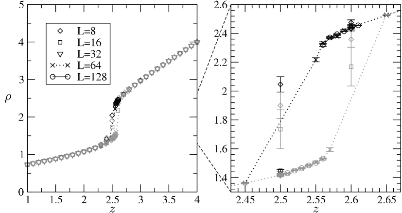
Figure 1: The measured values of $\rho$ as a function of $z$ for $q=10$ and $T=0$ using five different box sizes and $250+2500$ sweeps, all with both ordered (black) and disordered (grey) initial conditions. Only the equilibrated results have been shown, see the text for explanation.

The order of the transition was determined from the dependence of the observables on using either ordered or disordered initial conditions. If the different initial conditions led to different values of density, the transition was determined to be of first order. Our results also fully support the discussion made in section 3.2 which allows us to identify the two different results as properties of the different coexisting phases. Figures 1 and the $q=5$ part of 2 present typical examples of the behavior in these instances: both initial conditions lead to density fluctuations ${\cal O}\!\left(1/L\right)$, but the average values are separated by a constant ${\cal O}\!\left(1\right)$. (This is true only for large enough $L$. For very small $L$, there is a significant probability to jump from one density region to another, and then the result is some average of the values for each phase, and the standard deviation is of the order of the gap between these values.) In addition, the observed values are right-continuous for the ordered initial conditions, and left-continuous for the disordered ones.

In case the values agreed, we next looked at the behavior of $\rho^{\prime}$: since its maximum was then always found to diverge as some power of $L$ in a neighborhood of the percolation threshold, we call these second order transitions. In Figure 2 we have plotted the evolution of the density under our algorithm for the values in the borderline cases: the largest $q$ for which the transition was found to be of second order, $q=4$, and the smallest $q$ for which it was of first order, $q=5$.

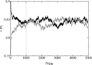
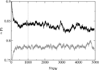
Figure 2: The evolution of $\rho/z$ under the algorithm for $q=4$ (the left figure) and $q=5$ (the right figure), and for two different initial conditions as described in the text: ordered (the black line) and disordered (the grey line). In all of these runs, $T=0$, $L=512$, and $z\approx z_{\text{c}}$ ($z=2.05125$ for $q=4$ and $z=2.168$ for $q=5$). $n_{\text{SW}}$ denotes the number of “sweeps” performed, and the dotted line represents the chosen equilibration cutoff, $n_{0}$.

In some cases, especially when using the “wrong” initial conditions near the borders of a first order transition region, the equilibration times turned out to be much longer than the chosen $n_{0}$ – see Figure 3 for a typical instance. Similar problems, combined with very long decorrelation times, plagued the $q=4$ simulations in large boxes as well; note, for instance, that $n_{0}=250$ is clearly insufficient for the left part in Figure 2. However, since typically only one of the initial conditions suffered from these long equilibration times, we decided, instead of redoing the simulations with very large $n_{0}$, to throw away the non-equilibrated value and use only the equilibrated one. This explains some of the apparently “missing points” in Figure 1. Nevertheless, we always kept at least one result for each $z$, redoing the simulations with larger $n_{0}$ when necessary.

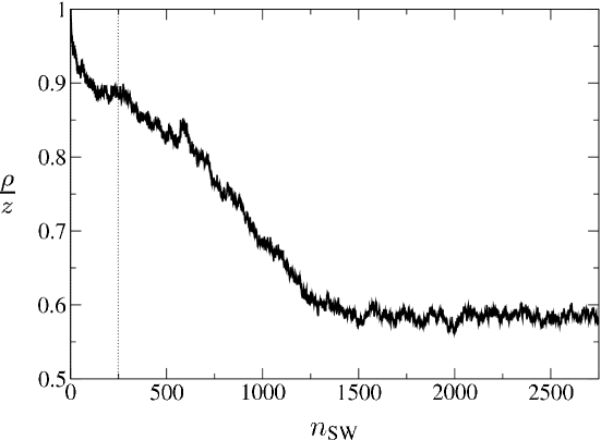
Figure 3: The evolution of $\rho/z$ for $q=10$, $T=0$, and $z=2.54$, using $L=128$ and ordered initial conditions. $n_{\text{SW}}$ denotes the number of sweeps performed, and the dotted line the preset equilibration cutoff.

	$T=0$			$T=0.5$
$q$	$z_{\text{c}}$		order	$z_{\text{c}}$		order
2	1.	718(7)	2nd	1.	86(4)	2nd
3	1.	907(8)	2nd	–		–
4	2.	051(4)	2nd	2.	273(7)	2nd
5	2.	1675(13)	1st	2.	424(2)	1st
10	2.	56(1)	1st	2.	965(25)	1st
50	3.	65(30)	1st	4.	95(65)	1st

Table 1: Estimates for the critical activity $z_{\text{c}}$ and the order of the transition in the $L\to\infty$ limit for several $q$ and at zero and one non-zero temperature. The error estimates are fairly conservative, see the text for how they were obtained from the simulations.

The results from this analysis are given in Table 1. For estimating finite-size effects, i.e., the difference of critical values from the $L\to\infty$ limit, we used certain monotonicity properties observed while doing the simulations. For second order transitions, the observable $\rho^{\prime}$ exhibits a divergence near the transition points, and the value quoted is the position of the maximum of the peak for the largest box size used. As can be seen also in Figure 4, this appears to increase monotonously with $L$, and therefore it can reasonably be taken as a lower bound for the limiting value. The error given, $\delta z_{c}$, is a value such that for $z\geq z_{c}+\delta z_{c}$ the measurements of $\rho^{\prime}$ for the two largest boxes agree with each other. Again, as seen in Figure 4, this is quite robust a value, fairly independent of $L$, and would in these cases be better understood as an upper bound for the error. For first order transitions, we used the property that the “coexistence window” between the disordered and ordered phase goes to zero as $L\to\infty$, apparently monotonously. In these cases, the error is given by the range of values in which both initial conditions were equilibrated but yielded differing results, plus one grid spacing. For instance, in the table we have $z_{c}=2.56(1)$ for $q=10$, $T=0$, which was obtained from the single coexistence value shown in Figure 1.

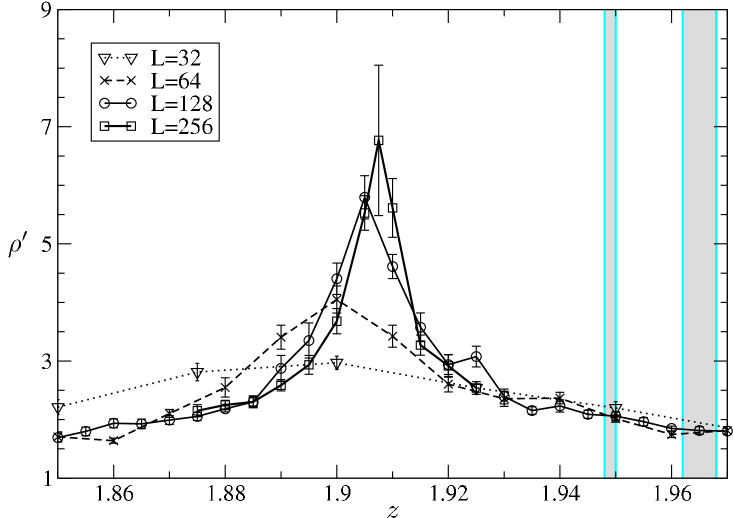
Figure 4: The measured values of $\rho^{\prime}$ as the function of $z$ for four different box sizes, computed for $q=3$ and $T=0$ using $250+2500$ sweeps. The value shown is an average of the results with ordered and disordered initial conditions. The shaded regions depict the results given in [12] for the critical $z$ with $L=160$ (left region) and with $L=40$ (right region).

5 Discussion

5.1 Comparison with earlier results

The Widom–Rowlinson and continuum Potts models have already been studied numerically before in [12] and [21]. These simulations used the so-called “invaded cluster” (IC) algorithm introduced in [16] for studying the lattice Potts models near criticality. This algorithm is similar to the Swendsen–Wang type of algorithms presented here. The main difference is that instead of generating samples for the finite volume Gibbs measure directly, a similar updating algorithm with a suitably chosen “stopping rule” is used for generating samples for a measure which differs from any of the finite volume Gibbs measures, but which is claimed to approach the correct Gibbs measure in the infinite volume limit.

The main advantage of the IC algorithm is that an advance scanning of the parameter space for finding the transition values is not necessary, as the stopping rule is assumed to be chosen so as to force the system to be at the transition point in the infinite volume limit. Two stopping rules are used in [12, 21] to study the continuum models: the percolation rule for $q\leq 3$ when the transition was expected to be of second order, and the fixed density rule for $q\geq 3$ to study whether the transition is of the first order. The main disadvantage of the IC algorithm is that the above mentioned convergence to the correct limit measure has not been proved so far and, in any case, it is quite difficult to control the finite size effects.

In Figure 4, we have compared the results for the critical activity $z_{c}$ for $q=3$ and $T=0$ from the present algorithm to those obtained using the percolating IC algorithm in [12]. The finite size effects appear to be more prominent in the percolating IC algorithm: by Figure 4 increasing the linear size fourfold from $L=40$ to $L=160$ does not appear even to halve the systematic error to the $L\to\infty$ value which we estimated (using lattice sizes up to $L=256$) from the position of the peak in $\rho^{\prime}$.

For $q=2$, $T=0$, we found for the limiting value $z_{c}=1.718(7)$, while in [12] $z_{c}=1.7262(4)$ for $L=160$, and $z_{c}=1.7201(7)$ for $L=40$ were measured. The finite size effects seem to be weaker in this case. In [21], simulations were performed also for a few non-zero temperatures. Unfortunately, there is only one instance in which we can directly compare our results with theirs: for $T=0.5$, $q=2$ we estimated $z_{c}(L=\infty)=1.86(4)$ while in [21] for $L=20$ with the same parameter values $z_{c}=1.8508(4)$ is given. Due to coarseness of our result, we cannot really compare the finite size effects in this case.

Let us offer a possible explanation for the observed differences between the results from these two methods. Since percolation (i.e., the existence of a cluster spanning the whole of $\Lambda$) was used as the stopping condition in the above quoted results, every sample configuration contains a percolating cluster. Even if we assume that samples approximating the infinite volume measure at the percolation threshold are generated by the IC-algorithm, this sampling method introduces some bias into the measurements. Actually, comparing the IC results with ours, it appears that the IC-method overestimates the critical activity $z_{c}$. This can be understood by observing that, in finite volume, the probability of having a percolating cluster is a continuous function of $z$ ascending from $0$ to $1$ around $z_{c}$, and thus is certainly not close to $1$ at $z_{c}$ but only when $z$ is sufficiently larger than $z_{c}$.

For first order transitions, we would expect exactly the opposite to happen: the percolating IC-algorithm should underestimate $z_{c}$. Indeed, since this algorithm produces only samples with a percolating cluster, the ordered phase gains an advantage over the disordered phase whenever there is a chance for it to occur. But, in finite volume, the ordered and disordered phases can coexist throughout a whole range of parameter values $z$ (rather than only at $z_{c}$, as in infinite volume). The threshold detected by the IC-algorithm therefore identifies only the lower end of the coexistence interval. Unfortunately, we cannot test this hypothesis, as the fixed-density stopping rule, and not the percolation one, was used in [21] for obtaining the critical activity for those $q$ exhibiting first order transitions.

Apart from these differences, our results confirm those found in [12] and [21]. For both the Widom–Rowlinson model ($T=0$) and the Potts model (at least with this particular non-zero temperature) we found only a single phase transition point, and the onset of percolation is an order parameter for this transition. As in these references, we also found that the transition is of second order for $q=2,3,4$, and of first order for $q\geq 5$.

5.2 Structure of pure phases

Apart from localizing the critical activity $z_{c}$ and clarifying the nature of the transition, our simulation measurements also provide some insight into the structure of the pure phases. Let us start by considering Figure 5 which shows the evolution of our observables $\rho$ (density), $\gamma$ (largest cluster size) and $d_{\text{perc}}$ (percolation distance) for $q=5$ during the simulation steps for two initial conditions: ordered (left-hand side) and disordered (right-hand side). It is clear that $\rho$ and $\gamma$ display more or less stationary fluctuations around some value that depends on the initial condition. This indicates the stability of the ordered and disordered phases over the observation period and allows to infer that these phases coexist; recall the discussion in Section 3.2. It also shows that the ordered phases have a higher particle density than the disordered phase, which means that the particle density in infinite volume should have a jump at $z_{c}$. Likewise, the proportion of particles in the largest cluster is nearly $1$ in the ordered case and nearly $0$ in the disordered case, from which we conclude that the typical configurations of the ordered phases contain a macroscopic cluster, while those of the disordered phase do not. A glance at the evolution of $d_{\text{perc}}$ reveals that, in the ordered case, the macroscopic cluster typically hits the central $4\times 4$ square. On the other hand, in the disordered case we see many “spikes”, telling that it can quite well happen that one can walk a long distance from the central $4\times 4$ square along the random graph, but the corresponding clusters are quite “fragile” and filamented, surviving only for a short time. All these effects become more pronounced when $q$ gets larger, as can be seen from Figure 6 for the case $q=10$.

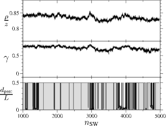
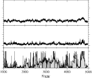
Figure 5: The evolution of the density, largest cluster size, and percolation distance, $\rho$, $\gamma$, and $d_{\text{perc}}$, respectively (see the text for precise definitions). Ordered initial conditions were used in the left case, disordered in the right, while otherwise in both cases $q=5$, $T=0$, $z=2.168\approx z_{\text{c}}$, and $L=512$.

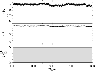
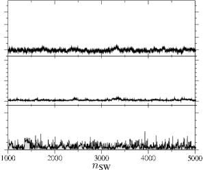
Figure 6: As in Figure 5, but for the case $q=10$, $T=0$, $z=2.56$, and $L=128$.

By way of contrast, Figures 7 and 8 show the corresponding structure in cases $q=2$ and $q=4$. It is obvious that essentially no difference can be found between the ordered and disordered initial conditions, and that the criticality of $z_{c}$ manifests itself only by very large fluctuations. We thus conclude that the phase transition is of second order. In fact, it also becomes clear that $q=4$ is a boundary case: the portion of particles in the largest cluster is typically quite large, and so is the percolation distance. This gives the hint that the onset of percolation at $z_{c}$ is quite rapid, and that the underlying value of $z$ in Figure 8 is actually slightly above $z_{c}$.

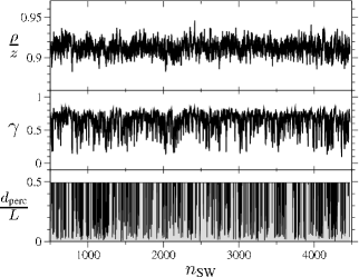
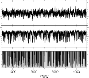
Figure 7: As in Figure 5, but for the case $q=2$, $T=0$, $z=1.72$, and $L=128$.

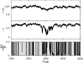
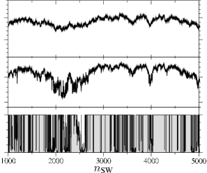
Figure 8: As in Figure 5, but for the case $q=4$, $T=0$, $z=2.05125$, and $L=512$.

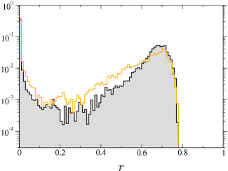
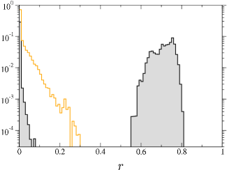
Figure 9: Histograms for the probabilities of finding a particle in a cluster which contains a portion $r$ of the particles. On the left, the data were obtained from the runs with $q=4$ depicted in Figure 8 with the shaded area giving the histograms for the ordered initial condition and the gray line for the disordered. The right figure shows the corresponding results for the $q=5$ runs given in Figure 5.

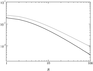
Figure 10: The probability of finding a particle in a cluster of size $s$. Measured from the same runs as the $q=5$ part of Figure 9, again black corresponding to the ordered initial condition and grey to the disordered one.

Figure 9 presents the cluster-size distributions in the second-order case $q=4$ and the first-order case $q=5$, again for ordered and disordered initial conditions. For $q=4$, there is again almost no influence of the initial conditions, while for $q=5$ there is a dramatic difference, and the different phases are separated by a range of values of cluster size which were not observed in either phase: those corresponding to the case when about half of the particles are in the maximal cluster. Finally, Figure 10 shows that in both phases the portion of particles in small clusters decays like a power-law of the cluster size (note the log-log scale in the figure). However, in the ordered phase the decay is clearly faster.

References

- [1] M. Aizenman, J. T. Chayes, L. Chayes, and C. M. Newman, The phase boundary in dilute and random Ising and and Potts ferromagnets, J. Phys. A 20 (1987), L313–L318.
- [2] J. Bricmont, K. Kuroda, and J.L. Lebowitz, First order phase transitions in lattice and continuous systems: Extension of Pirogov-Sinai theory, Commun. Math. Phys. 101 (1985), 501-538.
- [3] J. T. Chayes, L. Chayes, and R. Kotecký, The analysis of the Widom–Rowlinson model by stochastic geometric methods, Commun. Math. Phys. 172 (1995), 551–569.
- [4] L. Chayes, and J. Machta, Graphical representations and cluster algorithms, Part II, Physica A 254 (1998), 477–516.
- [5] A. Dembo, and O. Zeitouni, Large deviations techniques and applications, Boston London, Jones and Bartlett Publishers, 1993.
- [6] H.-O. Georgii, “Phase transition and percolation in Gibbsian particle models,” Statistical Physics and Spatial Statistics, The Art of Analyzing and Modeling Spatial Structures and Pattern Formation, Lecture Notes in Physics Vol. 554, Eds., K. L. Mecke, and D. Stoyan, 267-294. Springer, Berlin etc., 2000.
- [7] H.-O. Georgii and O. Häggström, Phase transition in continuum Potts models, Commun. Math. Phys. 181 (1996), 507–528.
- [8] H.-O. Georgii, O. Häggström and C. Maes, The random geometry of equilibrium phases, in: Phase Transitions and Critical Phenomena, C. Domb and J.L. Lebowitz (eds.), Academic Press (2000)
- [9] J. A. Given, and G. Stell, The Kirkwood-Salsburg equations for continuum percolation. J. Statist. Phys. 59 (1990), 981–1018.
- [10] O. Häggström, Random-cluster representations in the study of phase transitions, Markov Proc. Rel. Fields 4 (1998), 275–321.
- [11] O. Häggström, M. N. M. van Lieshout, and J. Møller, Characterization results and Markov chain Monte Carlo algorithms including exact simulation for some spatial point processes, Bernoulli 5 (1999), 641–658.
- [12] G. Johnson, H. Gould, J. Machta, and L. K. Chayes, Monte Carlo study of the Widom-Rowlinson fluid using cluster methods, Phys. Rev. Lett. 79 (1997), 2612–2615.
- [13] R. Kotecký, and S. Shlosman, First-order phase transitions in large entropy lattice systems, Commun. Math. Phys. 83 (1982), 493–550.
- [14] L. Laanait, A. Messager, S. Miracle-Solé, J. Ruiz, and S. Shlosman, Interfaces in the Potts model. I. Pirogov-Sinai theory of the Fortuin-Kasteleyn representation, Comm. Math. Phys. 140 (1991), 81–91.
- [15] J. L. Lebowitz, and E. H. Lieb, Phase transition in a continuum classical system with finite interactions, Phys. Lett. 39A (1972), 98–100.
- [16] J. Machta, Y. S. Choi, A. Lucke, T. Schweizer, and L. M. Chayes, Invaded cluster algorithm for Potts models, Phys. Rev. E 54 (1996), 1332–1345.
- [17] M. E. J. Newman and R. M. Ziff, Fast Monte Carlo algorithm for site or bond percolation, Phys. Rev. E 64 (2001), 016706:1–16.
- [18] R. B. Potts, Some generalized order–disorder transformations, Proc. Cambridge Phil. Soc. 48 (1952), 106-109
- [19] D. Ruelle, Existence of a phase transition in a continuous classical system. Phys. Rev. Lett. 27 (1971), 1040–1041.
- [20] F. H. Stillinger, Jr., and E. Helfand, Critical solution behavior in a binary mixture of Gaussian molecules, J. Chem. Phys. 41 (1964), 2495–2502.
- [21] R. Sun, H. Gould, J. Machta, and L. W. Chayes, Cluster Monte Carlo study of multicomponent fluids of the Stillinger-Helfand and Widom-Rowlinson type, Phys. Rev. E 62 (2000), 2226–2232.
- [22] R. H. Swendsen, and J.-S. Wang, Nonuniversal critical dynamics in Monte Carlo simulations, Phys. Rev. Lett. 58 (1987), 86–88.
- [23] B. Widom, and J. S. Rowlinson, New model for the study of liquid-vapor phase transition, J. Chem. Phys. 52 (1970), 1670–1684.