Quantum diffusion for the Anderson model
in the scaling limit.

Abstract

We consider random Schrödinger equations on ${\mathbb{Z}}^{d}$ for $d\geq 3$ with identically distributed random potential. Denote by $\lambda$ the coupling constant and $\psi_{t}$ the solution with initial data $\psi_{0}$. The space and time variables scale as $x\sim\lambda^{-2-\kappa/2},t\sim\lambda^{-2-\kappa}$ with $0<\kappa<\kappa_{0}(d)$. We prove that, in the limit $\lambda\to 0$, the expectation of the Wigner distribution of $\psi_{t}$ converges weakly to a solution of a heat equation in the space variable $x$ for arbitrary $L^{2}$ initial data. The diffusion coefficient is uniquely determined by the kinetic energy associated to the momentum $v$.

This work is an extension to the lattice case of our previous result in the continuum [8], [9]. Due to the non-convexity of the level surfaces of the dispersion relation, the estimates of several Feynman graphs are more involved.

AMS 2000 Subject Classification: 60J65, 81T18, 82C10, 82C44

1 Introduction

We consider the time evolution of the Anderson model [2] given by the random Schrödinger equation

$$i\partial_{t}\psi_{t}(x)=H\psi_{t}(x),\qquad\psi_{t}\in\ell^{2}({\mathbb{Z}}^{d}),\;\;t\in{\mathbb{R}}$$ (1.1)

on the $d$-dimensional square lattice ${\mathbb{Z}}^{d}$. The Hamiltonian is given by

$$H=-\frac{1}{2}\Delta+\lambda V_{\omega}\;,$$ (1.2)

where $\lambda>0$ is the coupling constant. The kinetic energy operator on $\ell^{2}(\mathbb{Z}^{d})$ is given by

$$(\Delta f)(x):=2d\;f(x)-\sum_{|e|=1}f(x+e)$$ (1.3)

and the random potential is given by

$$V_{\omega}(x)=\sum_{\alpha\in{\mathbb{Z}}^{d}}V_{\alpha}(x)\qquad V_{\alpha}(x):=v_{\alpha}\;\delta_{x,\alpha}$$ (1.4)

where $\{v_{\alpha}\;:\;\alpha\in{\mathbb{Z}}^{d}\}$ are i.i.d. random variables and $\delta_{x,\alpha}={\bf 1}\{x=\alpha\}$ is the usual Kronecker delta function and ${\bf 1}\{\cdot\}$ is the characteristic function. We will work in $d=3$ dimension, but our results and proofs extend to any $d\geq 3$ in a straight-forward manner.

We study the long time evolution of the equation (1.1). For a large coupling constant, $\lambda\geq\lambda_{0}$, the spectrum of $H$ is almost surely pure point and the dynamics is localized [2, 11, 1]. It is conjectured, but not yet proven, that the spectrum is absolutely continuous and the dynamics is diffusive if $\lambda<\lambda_{0}$ is sufficiently small. We will investigate the dynamics in this regime in the scaling limit, when time diverges as $\lambda\to 0$.

Up to time scales $t\sim\lambda^{-2}$ the dynamics is kinetic, typically with a finite number of collisions. The evolution on macroscopic space scales, $x\sim\lambda^{-2}$, is given by a linear Boltzmann equation [13, 6, 3, 12]. As the long time limit of the Boltzmann equation is the heat equation, the quantum evolution on scales $t\gg\lambda^{-2}$ is expected to exhibit diffusive behavior. In this paper we prove this statement up to time scale $t\sim\lambda^{-2-\kappa}$ with a positive $\kappa$.

We have proved the same statement (with a somewhat bigger $\kappa$) for a random Schrödinger operator in the continuum, ${\mathbb{R}}^{d}$ [8, 9]. The history of this problem and related works are summarized in [8] and will not be repeated here.

Our reasons to extend this work to the lattice case are: (i) to show that the methods initiated in [6, 5], and later developed in [8, 9] for longer time scales, can be applied to a lattice setting as well; (ii) to make a connection with the extended state conjecture of the Anderson model.

Anderson (de)localization is a large distance phenomenon, thus no physical difference is expected between the lattice and continuum models. The localization proofs, however, are typically simpler in the lattice models because of certain technical difficulties due to the ultraviolet regime in the continuum model.

We now explain briefly the differences between the continuum and lattice models in our analysis of the delocalization regime. The finite momentum space is an advantage in this regime as well; the artificial large momentum cutoffs introduced for the continuum model in [8] are not necessary here. Moreover, the computation of the main term is more direct since the Boltzmann collision kernel is homogeneous on the energy shells (compare (2.19) below with (2.19) of [8]). In particular, the diffusion coefficient can be computed explicitly.

However, an important technical estimate is considerably more involved for the lattice case. The complication stems from the non-convexity of the isoenergy surfaces of the lattice Laplacian. The isoenergy surfaces are the level sets, $\Sigma_{\alpha}:=\{p\in{\bf T}^{d}\;:\;e(p)=\alpha\}$, of the dispersion relation

$$e(p):=\sum_{j=1}^{d}\big{(}1-\cos(2\pi p^{(j)})\big{)},\qquad p=(p^{(1)},\ldots,p^{(d)})\in{\bf T}^{d}:=\Big{[}-\frac{1}{2},\frac{1}{2}\Big{]}^{d}\;.$$ (1.5)

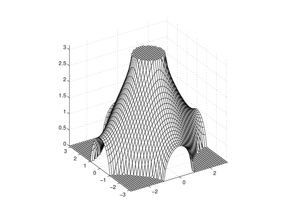
Figure 1: Level set of $e(p)=\alpha$ for $2<\alpha<4$

Our approach heavily uses estimates that integrals of resolvent functions, $|\alpha-e(p)+i\eta|^{-1}$, $\eta\ll 1$ are concentrated near $\Sigma_{\alpha}$. In particular, our most involved estimate (Four Denominator Lemma 3.4) translates naturally to a specific decay property of the Fourier transform of measures supported on the hypersurfaces $\Sigma_{\alpha}$. Such decay bounds are readily available for surfaces with non-vanishing Gauss curvature, but we were unable to find in the literature the necessary estimate for surfaces with Gauss curvature vanishing along a submanifold. Since in the energy range $\alpha\in(2,2d-2)$, the Gaussian curvature of the level sets $\Sigma_{\alpha}$ vanish along a codimension one submanifold (see Figure 1), we had to prove this estimate separately [10]. Another related bound (Two Denominator Lemma 7.7) will be proven in this paper.

The analogous bounds in the continuum model, with dispersion relation $e(p)=\frac{1}{2}p^{2}$, are much easier. The actual proofs (e.g. Proposition 2.3 in [4] or Lemma A.1 in [8]) use the explicit form of $e(p)$, but the key fact is that the level sets of the dispersion relation are convex.

Most importantly, the Two-Denominator Lemma is much stronger in the continuum case; the estimate in Lemma 7.7 carries a diverging factor $\eta^{-3/4-\kappa}$. The corresponding bound (formula (10.28) in [8]) is only logarithmically divergent in $d=3$. This makes the estimates of the error terms in [9] much easier.

We mention that the difficulty related to the non-convexity of the level sets is present in the proofs of the Boltzmann equation from a lattice model [3, 12] as well. On the kinetic time scale, however, weaker bounds (called crossing estimates) were sufficient (Lemma 7.8 of [3] or Assumption (DR4) of [12]).

The main inputs we use from our other works are: (i) the stopping rules (Section 3 of [9]); (ii) the basic integration procedure for non-repetition Feynman graphs (Sections 8-10 of [8]); (iii) the organization of the estimates on the error terms (Section 4 of [9]); and (iv) the Four Denominator Lemma proved in [10]. The new ingredients are: (i) the estimates of the error terms (with the Four Denominator Lemma replacing the strong form of the Two Denominator Lemma not available in the lattice case); (ii) the computation of the main term and the explicit diffusion coefficient.

2 Statement of the main result

2.1 Notations

In this paper we consider the random Schrödinger operator (1.2) acting on $\ell^{2}({\mathbb{Z}}^{d})$. The kinetic energy operator is given by the discrete Laplacian (1.3) and $V_{\omega}(x)$ is the random potential (1.4). Denote the moments of the single-site random potential by $m_{k}={\bf E}\;v_{\alpha}^{k}$. We assume that $m_{1}=m_{3}=m_{5}=0$, $m_{6}<\infty$, and $m_{2}=1$ by normalization. Universal constants will be denoted by $C$ and their value may vary from line to line.

On the lattice $(\delta{\mathbb{Z}})^{d}$, $\delta>0$, we introduce the notation

$$\int_{(\delta{\mathbb{Z}})^{d}}(\cdots){\rm d}x:=\delta^{d}\sum_{x\in(\delta{\mathbb{Z}})^{d}}(\cdots)\;.$$ (2.1)

On the dual space $({\bf T}/\delta)^{d}$, with ${\bf T}:=[-\frac{1}{2},\frac{1}{2}]$, the integration refers to the usual Lebesgue integral

$$\int_{({\bf T}/\delta)^{d}}(\cdots){\rm d}p\;.$$ (2.2)

We will use these formulas mostly for $\delta=1$ in which case we will drop the subscripts $(\delta{\mathbb{Z}})^{d}$ and $({\bf T}/\delta)^{d}$ indicating the integration domains in (2.1), (2.2). The letters $x,y,z$ will always denote lattice variables, while $p,q,r,u,v,w$ will be reserved for $d$-dimensional momentum variables on the torus. This notation will distinguish between the two integrations (2.1) and (2.2). Note that as $\delta\to 0$, both integrals converge to the standard Lebesgue integral on ${\mathbb{R}}^{d}$.

For any $f\in\ell^{2}((\delta{\mathbb{Z}})^{d})$ the Fourier transform is given by

$$\widehat{f}(p)\equiv({\cal F}f)(p):=\int_{(\delta{\mathbb{Z}})^{d}}e^{-2\pi ip\cdot x}f(x){\rm d}x=\delta^{d}\sum_{x\in(\delta{\mathbb{Z}})^{d}}e^{-2\pi ip\cdot x}f(x)\;,$$ (2.3)

where $p=(p^{(1)},\dots,p^{(d)})\in({\bf T}/\delta)^{d}$. The inverse Fourier transform is given by

$$({\cal F}^{-1}\widehat{g})(x)=\int_{({\bf T}/\delta)^{d}}\widehat{g}(p)e^{2\pi ip\cdot x}{\rm d}p\;.$$

The notations ${\cal F}(\cdot)$ and $\widehat{(\cdot)}$ will be used according to convenience. For functions defined on the phase space, $f(x,v)$, with $x\in(\delta{\mathbb{Z}})^{d}$, $v\in({\bf T}/\delta)^{d}$, the Fourier transform will always be taken only in the space variable, i.e.

$$\widehat{f}(\xi,v):=\int_{(\delta{\mathbb{Z}})^{d}}e^{-2\pi i\xi\cdot x}f(x,v){\rm d}x,\quad\xi\in({\bf T}/\delta)^{d}\;.$$

We also remark that addition and subtraction of momenta will always be defined on the torus, i.e. with periodic boundary conditions.

The Fourier transform of the kinetic energy operator (1.3) on $\ell^{2}({\mathbb{Z}}^{d})$ is given by

$$({\cal F}\Delta f)(p)=-2e(p)\widehat{f}(p)\;,$$

where $e(p)$ is the dispersion law defined in (1.5). For $h:{\bf T}^{d}\to{\bf C}$ and an energy value $e\in[0,2d]$ we introduce the notation

$$[h](e):=\int h(v)\delta(e-e(v)){\rm d}v:=\int_{\Sigma_{e}}h(q)\;\frac{{\rm d}\nu(q)}{|\nabla e(q)|}$$ (2.4)

where ${\rm d}\nu(q)={\rm d}\nu_{e}(q)$ is the restriction of the $d$-dimensional Lebesgue measure to the level surface

$$\Sigma_{e}:=\{q\;:\;e(q)=e\}\subset{\bf T}^{d}.$$

By the co-area formula it holds that

$$\int_{0}^{2d}[h](e){\rm d}e=\int h(v){\rm d}v\;.$$ (2.5)

We define the projection to the energy space of the free Laplacian by

$$\langle\,h(v)\,\rangle_{e}:=\frac{[h](e)}{\Phi(e)}\;,\quad\mbox{ where }\quad\Phi(e):=[1](e)=\int\delta(e-e(u)){\rm d}u\;.$$ (2.6)

Define the Wigner transform of a function $\psi\in\ell^{2}(\mathbb{Z}^{d})$

$$W_{\psi}(x,v):=2^{d}\sum_{y,z\in{\mathbb{Z}}^{d}\atop y+z=2x}e^{2\pi iv\cdot(y-z)}\overline{\psi(y)}\psi(z),\qquad x\in\Big{(}\frac{{\mathbb{Z}}}{2}\Big{)}^{d},\;v\in{\bf T}^{d}\;.$$ (2.7)

Notice that the position variable $x$ takes values on the refined lattice $({\mathbb{Z}}/2)^{d}$. It is easy to compute the Fourier transform of $W_{\psi}(x,v)$ in $x$ using (2.3) with $\delta=1/2$, and one obtains

$$\widehat{W}_{\psi}(\xi,v)=\overline{\widehat{\psi}\Big{(}v-\frac{\xi}{2}\Big{)}}\widehat{\psi}\Big{(}v+\frac{\xi}{2}\Big{)}\;,\qquad\xi\in(2{\bf T})^{d},\;v\in{\bf T}^{d}\;.$$ (2.8)

Note that $\widehat{W}_{\psi}(\xi,v)$ is periodic with respect to the double torus $(2{\bf T})^{d}$. It is easy to check that $W_{\psi}(x,v)$ reproduces the correct marginals in the following sense

$$\int W_{\psi}(x,v){\rm d}v=\left\{\begin{array}[]{cl}2^{d}|\psi(x)|^{2}&\mbox{if}\;\;x\in{\mathbb{Z}}^{d}\\ 0&\mbox{if}\;\;x\in({\mathbb{Z}}/2)^{d}\setminus{\mathbb{Z}}^{d}\end{array}\right.$$

$$\int_{({\mathbb{Z}}/2)^{d}}W_{\psi}(x,v){\rm d}x=2^{-d}\sum_{x\in({\mathbb{Z}}/2)^{d}}W_{\psi}(x,v)=|\widehat{\psi}(v)|^{2}\;,$$ (2.9)

and in particular

$$\int_{({\mathbb{Z}}/2)^{d}}\int W_{\psi}(x,v){\rm d}v{\rm d}x=\|\psi\|^{2}\;.$$

Recall that momentum integrations on unspecified domains are always considered on ${\bf T}^{d}$. Define the rescaled Wigner distribution as

$$W^{\varepsilon}_{\psi}(X,V):=\varepsilon^{-d}W_{\psi}\Big{(}\frac{X}{\varepsilon},V\Big{)}\;,\quad X\in(\varepsilon{\mathbb{Z}}/2)^{d},\;V\in{\bf T}^{d}\;.$$ (2.10)

Its Fourier transform in $X$ is given by

$$\widehat{W}^{\varepsilon}_{\psi}(\xi,V)={\cal F}\big{(}W^{\varepsilon}_{\psi}(\;\cdot\;,V)\big{)}(\xi)=\overline{\widehat{\psi}\Big{(}V-\frac{\varepsilon\xi}{2}\Big{)}}\widehat{\psi}\Big{(}V+\frac{\varepsilon\xi}{2}\Big{)}\;,\quad\xi\in(2{\bf T}/\varepsilon)^{d},\;V\in{\bf T}^{d}\;.$$

To test the rescaled Wigner transform against a Schwarz function ${\cal O}(x,v)$ on ${\mathbb{R}}^{d}\times{\bf T}^{d}$, we introduce the scalar products:

$$\langle\,{\cal O},W_{\psi}^{\varepsilon}\rangle: =\int_{(\varepsilon{\mathbb{Z}}/2)^{d}}{\rm d}X\int{\rm d}v\;{\cal O}(X,v)W_{\psi}^{\varepsilon}(X,v)$$

$$\langle\,\widehat{\cal O},\widehat{W}_{\psi}^{\varepsilon}\rangle: =\int_{(2{\bf T}/\varepsilon)^{d}}{\rm d}\xi\int{\rm d}v\;\widehat{\cal O}(\xi,v)\overline{\widehat{W}_{\psi}^{\varepsilon}}(\varepsilon\xi,v)\;.$$ (2.11)

By unitarity of the Fourier transform, $\langle\,{\cal O},W_{\psi}^{\varepsilon}\rangle=\langle\,\widehat{\cal O},\widehat{W}_{\psi}^{\varepsilon}\rangle$.

One may, of course, also define the Wigner transform of a function $\psi\in\ell^{2}({\mathbb{Z}}^{d})$ by first defining $\widehat{W}_{\psi}(\xi,v)$ for $\xi\in(2{\bf T})^{d}$ by (2.8), then taking the inverse Fourier transform in $\xi$ to reproduce the lattice function defined in (2.7). An interpretation of the Wigner function as a distribution starting from (2.8) for any $\xi\in{\mathbb{R}}^{d}$ was given in [12].

2.2 Main theorem

The weak coupling limit is defined by the following scaling:

$${\cal T}:=\varepsilon t,\quad{\cal X}:=\varepsilon x,\quad\varepsilon=\lambda^{2}\;.$$ (2.12)

It was proved [3] that in the limit $\varepsilon\to 0$ the Wigner distribution $W^{\varepsilon}_{\psi_{{\cal T}/\varepsilon}}({\cal X},{\cal V})$ converges weakly to the solution of the Boltzmann equation

$$\partial_{\cal T}F_{\cal T}({\cal X},V)+\sin(2\pi V)\cdot\nabla_{\cal X}F_{\cal T}({\cal X},V)$$

$$\hskip 56.9055pt=2\pi\int{\rm d}U\delta(e(U)-e(V))\Big{[}F_{\cal T}({\cal X},U)-F_{\cal T}({\cal X},V)\Big{]}\;,$$ (2.13)

with velocity vector $\sin(2\pi V):=(\sin(2\pi V_{1}),\sin(2\pi V_{2}),\sin(2\pi V_{3}))=\frac{1}{2\pi}\nabla e(V)$. Here ${\cal F}_{\cal T}({\cal X},{\cal V})$ is the time dependent limiting phase space density with ${\cal X}\in{\mathbb{R}}^{d}$, ${\cal V}\in{\bf T}^{d}$. Note that the Boltzmann equation can be viewed as the generator of a Markovian semigroup on phase space. In particular, all correlation effects become negligible in this scaling limit.

In this paper we consider the long time scaling

$$x=\lambda^{-\kappa/2-2}X=\varepsilon^{-1}X,\quad t=\lambda^{-\kappa-2}T=\varepsilon^{-1}\lambda^{-\kappa/2}T,\quad\varepsilon=\lambda^{\kappa/2+2}\;$$ (2.14)

with $\kappa>0$. Our main result is the following theorem.

Theorem 2.1

Let $d=3$ and $\psi_{0}\in\ell^{2}({\mathbb{Z}}^{d})$ be an initial wave function. Let $\psi(t)=\psi_{t,{\omega}}^{\lambda}$ solve the Schrödinger equation (1.1). Let ${\cal O}(x,v)$ be a Schwarz function on ${\mathbb{R}}^{d}\times{\bf T}^{d}$. For almost all energies $e\in[0,2d]$, $\big{[}|\widehat{\psi}_{0}(v)|^{2}\big{]}(e)$ is finite and for these energies let $f$ be the solution to the heat equation

$$\partial_{T}f(T,X,e)=\;\nabla_{X}\cdot D(e)\nabla_{X}f(T,X,e)$$ (2.15)

with the initial condition

$$f(0,X,e):=\delta(X)\Big{[}|\widehat{\psi}_{0}(v)|^{2}\Big{]}(e)$$

and the diffusion matrix $D$

$$D_{ij}(e):=\frac{\big{\langle}\,\sin(2\pi v^{(i)})\cdot\sin(2\pi v^{(j)})\,\big{\rangle}_{e}}{2\pi\;\Phi(e)}\;\qquad i,j=1,2,3.$$ (2.16)

Then for $\kappa<\kappa_{0}$ and $\varepsilon$ and $\lambda$ related by (2.14), the Wigner distribution satisfies

$$\lim_{\varepsilon\to 0}\int_{(\varepsilon{\mathbb{Z}}/2)^{d}}\!\!{\rm d}X\!\int\!{\rm d}v\;{\cal O}(X,v){\bf E}W^{\varepsilon}_{\psi(\lambda^{-\kappa-2}T)}(X,v)=\int_{{\mathbb{R}}^{d}}{\rm d}X\int\!\!{\rm d}v\;{\cal O}(X,v)f(T,X,e(v))\;,$$ (2.17)

and the limit is uniform on $T\in[0,T_{0}]$ with any fixed $T_{0}$. In $d=3$ dimensions, one can choose $\kappa_{0}=1/9800$.

Remarks. (i) We stated the Theorem and will carry out the proof in $d=3$ for simplicity but our method works for any $d\geq 3$.

(ii) The analogous theorem for the continuum model was proved in [8] and [9] with a somewhat larger threshold for $\kappa$. The threshold is obtained from technical estimates, it has no physical relevance and it can be improved with a more careful analysis.

(iii) By the symmetry of the measure $\langle\cdot\rangle_{e}$ under each sign flip $v_{j}\to-v_{j}$ and by the permutational symmetry of the coordinate axes, we see that $D(e)$ is a constant times the identity matrix:

$$D_{ij}(e)=D_{e}\;\delta_{ij},\qquad D_{e}:=\frac{\big{\langle}\sin^{2}(2\pi v^{(1)})\,\big{\rangle}_{e}}{2\pi\;\Phi(e)}\;,$$

in particular we see that the diffusion is nondegenerate.

(iv) The diffusion matrix can also be obtained from the long time limit of the Boltzmann equation (2.2) (see also the explanation to Figure 1 in [8]). For any fixed energy $e$, let

$$L_{e}f(v):=\int{\rm d}u\;\sigma(u,v)[f(u)-f(v)],\qquad e(v)=e\;,$$ (2.18)

be the generator of the momentum jump process on $\Sigma_{e}$ with the uniform stationary measure $\langle\cdot\rangle_{e}$. The collision kernel is

$$\sigma(U,V):=2\pi\delta(e(U)-e(V)).$$ (2.19)

The diffusion matrix in general is given by the velocity autocorrelation function

$$D_{ij}(e)=\int_{0}^{\infty}{\rm d}t\;\big{\langle}\sin(2\pi v^{(i)}(t))\cdot\sin(2\pi v^{(j)}(0))\big{\rangle}_{e}\;,$$ (2.20)

where $v(t)$ is the process generated by $L_{e}$. Since for any fixed $V$ the collision kernel $\sigma(U,V)$, is symmetric on the energy surface in the $U$ variable, the correlation between $v(t)$ and $v(0)$ vanishes after the first jump and we obtain (2.16), by using

$$\int{\rm d}u\;\sigma(u,v)=2\pi\Phi(e)\;,\qquad e(v)=e\;.$$

3 Preparations

3.1 Renormalization

The purpose of this procedure is to include immediate recollisions with the same obstacle into the propagator itself. Without renormalization, these graphs are exponentially large (“divergent”), but their sum is finite. Renormalization removes this instability and the analysis of the resulting Feynman graphs will become simpler.

The self-energy operator is given by the multiplication operator in momentum space

$$\theta(p):=\Theta(e(p)),\qquad\Theta(\alpha):=\lim_{\varepsilon\to 0+}\Theta_{\varepsilon}(\alpha)\;,$$ (3.1)

where

$$\Theta_{\varepsilon}(\alpha):=\int\frac{{\rm d}q}{\alpha-e(q)+i\varepsilon}\;.$$ (3.2)

The existence of the limit and related properties of $\Theta$ are proved in Lemma A.1

We rewrite the Hamiltonian as

$$H=H_{0}+\widetilde{V},$$

where

$$H_{0}:=\omega(p):=e(p)+\lambda^{2}\theta(p),\qquad\widetilde{V}:=\lambda V-\lambda^{2}\theta(p)\;.$$ (3.3)

We note that our renormalization is only an approximation to the standard self-consistent renormalization given by the solution to the equation

$${\omega}(p)=e(p)+\lambda^{2}\lim_{\varepsilon\to 0+0}\int\frac{{\rm d}q}{{\omega}(p)-{\omega}(q)+i\varepsilon}\;.$$ (3.4)

Due to our truncation procedure, the definition (3.1) is sufficient and is more convenient for us.

We also need a few properties of the function ${\omega}(p)$. First, ${\omega}(p)$ is symmetric under the permutation of the coordinate axes. Second, $e(p)$ is symmetric for reflections onto any coordinate axis: $e(p^{(1)},\ldots,p^{(d)})=e(\pm p^{(1)},\ldots,\pm p^{(d)})$ for any choices of the signs and these properties are inherited by $\theta(p)$ and ${\omega}(p)$. Moreover, $e({\bf\frac{1}{2}}-p)=2d-e(p)$, where ${\bf\frac{1}{2}}:=(\frac{1}{2},\frac{1}{2},\ldots,\frac{1}{2})$. Therefore $\Theta(\alpha)=-\overline{\Theta}(2d-\alpha)$ and

$$\theta({\bf\frac{1}{2}}-p)=-\overline{\theta(p)}\;.$$ (3.5)

These relations allow us to restrict our attention to the subdomain

$${\cal D}:=\Big{\{}p=(p^{(1)},p^{(2)},\ldots,p^{(d)})\in{\bf T}^{d}\;:\;0\leq p^{(1)}\leq p^{(2)}\leq\ldots\leq p^{(d)}\;,\sum_{j}p^{(j)}\leq\frac{d}{4}\Big{\}}$$ (3.6)

of the momentum space. On this domain we have the following estimate on $\theta(p)$:

Lemma 3.1

For any $d\geq 3$ there exist universal positive constants $c_{1},c_{2}$ such that

$$|\theta(p)|\leq c_{2}\;,$$ (3.7)

$$-c_{2}|p|^{d-2}\leq\mbox{Im}\;\theta(p)\leq-c_{1}|p|^{d-2}$$ (3.8)

for any $p\in{\cal D}$.

Using this bound and the symmetry properties of ${\omega}(p)$ above, we easily arrive at

Corollary 3.2

For $d\geq 3$ we have

$$\mbox{Im}\;{\omega}(p)\leq-c_{3}\lambda^{2}[D(p)]^{d-2},\qquad p\in{\bf T}^{d}$$ (3.9)

for some $c_{3}>0$, where

$$D(p):=\min\Big{\{}|p-v|\;:\;v=0\;\;\mbox{or}\;\;v=\Big{(}\pm\frac{1}{2},\;\pm\frac{1}{2},\ldots,\pm\frac{1}{2}\Big{)}\;\Big{\}}$$

is the distance between $p$ and the set consisting of the origin and the vertices of ${\bf T}^{d}$. $\;\;\Box$

We remark that this estimate would produce logarithmic corrections in $d=2$ dimensions, this is one of the reasons why the proof is somewhat simpler in $d\geq 3$.

Proof of Lemma 3.1. By the co-area formula (2.5) and recalling the definition (2.6) we can write $\Theta_{\varepsilon}(\alpha)$ as

$$\Theta_{\varepsilon}(\alpha)=\int_{0}^{2d}\frac{{\rm d}s}{\alpha-s+i\varepsilon}\;\Phi(s)\;,\qquad\mbox{with}\quad\Phi(s)=\int_{\Sigma_{s}}\frac{{\rm d}\nu(q)}{|\nabla e(q)|}\;.$$ (3.10)

Because of the symmetries of $e(q)$, it is sufficient to study

$$\widetilde{\Phi}(s):=\int_{\Sigma_{s}\cap{\cal D}}\frac{{\rm d}\nu(q)}{|\nabla e(q)|}\;,$$

i.e. where the integration is restricted to ${\cal D}$.

The critical values of $e(q)$ are the even integers, $2m$, between 0 and $d$, and within ${\cal D}$ they correspond to the critical points

$$p_{m}=\Big{(}0,0,\ldots,0,\underbrace{\frac{1}{2},\ldots,\frac{1}{2}}_{m\;\;\mbox{times}}\;\Big{)}$$

with $m\leq d/2$. If $s$ is away from a neighborhood of the critical values of $e(q)$, then $\Phi(s)$ is a bounded function with a strictly positive lower bound.

If $s$ is near a critical value, $s=2m+\beta$ with $\beta$ sufficiently small, then we can write

$$\widetilde{\Phi}(s)=\int_{\Sigma_{s}\cap{\cal D}}\frac{\chi_{m}(q)}{|\nabla e(q)|}\;{\rm d}\nu(q)+\int_{\Sigma_{s}\cap{\cal D}}\frac{1-\chi_{m}(q)}{|\nabla e(q)|}\;{\rm d}\nu(q)$$

where $\chi_{m}$ is a smooth cutoff function around the critical point $p_{m}$. The second integral is a regular function in $s$ that is separated away from 0. The first integral can be brought into the following normal form by a smooth local coordinate transformation:

$$\Phi^{\#}(\beta):=\int_{C(\beta)}\frac{\chi(q)}{|q|}\;{\rm d}q\;,$$

where $\chi$ is a smooth cutoff function around 0 and

$$C(\beta):=\Big{\{}q\in{\mathbb{R}}^{d}\;:\;\sum_{j=1}^{d-m}[q^{(j)}]^{2}-\sum_{j=d-m+1}^{d}[q^{(j)}]^{2}=\beta\;\Big{\}}\;.$$

It is a straightforward calculation to see the following behavior of the function $\Phi^{\#}>0$ for small $\beta$

$$\Phi^{\#}(\beta)=O\Big{(}\beta^{\frac{d}{2}-1}\Big{)},\qquad\frac{{\rm d}}{{\rm d}\beta}\Phi^{\#}(\beta)=O\Big{(}\beta^{\frac{d}{2}-2}\Big{)}\;\;\;\mbox{if}\;\;\;m=0$$ (3.11)

$$\Phi^{\#}(\beta)=O(1),\qquad\frac{{\rm d}}{{\rm d}\beta}\Phi^{\#}(\beta)=O(1)\;\;\;\mbox{if}\quad 1\leq m\leq d/2.$$

From these estimates, $\Phi$ is differentiable away from 0, bounded everywhere and $\Phi(s)$ behaves as $s^{1/2}$ near 0 in $d=3$ dimensions. For higher dimensions $\Phi^{\prime}$ is bounded. From the formula (3.10), we can rewrite $\Theta$ as

$$\Theta_{\varepsilon}(\alpha)=\int^{\alpha}_{\alpha-2d}\frac{{\rm d}s}{s+i\varepsilon}\;\Phi(\alpha-s)\;.$$ (3.12)

Using the above properties of $\Phi$ we can take the limit $\varepsilon\to 0$ and define $\Theta(\alpha):=\lim_{\varepsilon\to 0+0}\Theta_{\varepsilon}(\alpha)$. If we write $\Theta(e)={\cal R}(e)-i{\cal I}(e)$, where ${\cal R}(e)$ and ${\cal I}(e)$ are real functions, and recall $Im(x+i0)^{-1}=-\pi\delta(x)$, we have

$$\mbox{Im}\,\Theta(\alpha)=-\pi\int\delta(e(q)-\alpha){\rm d}q=-\pi\Phi(\alpha)\;.$$ (3.13)

Using the properties of $\Phi$, we can also check that for any $0\leq e\leq d$

$$\Phi(e)=f(e)e^{\frac{d}{2}-1},\qquad{\cal R}(e)=a(e)(1+e^{\frac{d}{2}-1}),\qquad{\cal I}(e)=b(e)e^{\frac{d}{2}-1}$$ (3.14)

where $a,b,f$ are bounded functions, uniformly separated away from zero and $f(e)>0$. We also have ${\cal I}(\alpha)=\pi\Phi(\alpha)$. The estimates in Lemma 3.1 then follow from the fact that $e(p)\geq cp^{2}$ on ${\cal D}$. Later we will also need the bounds

$$|\Phi^{\prime}(e)|\leq C(1+e^{\frac{d}{2}-2})\qquad|\Theta^{\prime}(e)|\leq|{\cal R}^{\prime}(e)|+|{\cal I}^{\prime}(e)|\leq C(1+e^{\frac{d}{2}-2})\;,$$ (3.15)

that can be proven by a similar analysis. $\;\;\;\Box$

The following lemma collects some estimates on the renormalized propagators we shall use to prove Theorem 2.1. Its proof will be given in the Appendix. These are technical bounds and their meanings will become clear when they are used.

Lemma 3.3

Suppose that $\lambda^{2}\geq\eta\geq\lambda^{2+4\kappa}$ with $\kappa\leq 1/12$. Then we have,

$$\sup_{\alpha}\int\frac{{\rm d}p}{|\alpha-{\omega}(p)+i\eta|}\leq C|\log\lambda|\;$$ (3.16)

and for $0\leq a<1$

$$\sup_{\alpha}\int\frac{{\rm d}p}{|\alpha-{\omega}(p)+i\eta|^{2-a}}\leq C_{a}\lambda^{-2(1-a)}.$$ (3.17)

For $a=0$, the following more precise estimate holds. There exists a universal constant $C_{0}$ such that

$$\begin{split}\sup_{\alpha}\int\frac{\lambda^{2}\;{\rm d}p}{|\alpha-\overline{\omega}(p)-i\eta|^{2}}&\leq 1+C_{0}\lambda^{1-12\kappa}\\ \sup_{\alpha,\beta,r}\int\frac{\lambda^{2}\;{\rm d}p}{|\alpha-\overline{\omega}(p+r)-i\eta|\;|\beta-{\omega}(p-r)+i\eta|}\;&\leq 1+C_{0}\lambda^{1-12\kappa}\;.\end{split}$$ (3.18)

3.2 Truncation

For any real number $\alpha$ we define

$$|\!|\!|\alpha|\!|\!|:=\min\{|\alpha|,|\alpha-2|,|\alpha-3|,|\alpha-4|,|\alpha-6|\}\;$$ (3.19)

in the $d=3$ dimensional model. The values $0,2,4,6$ are the critical values of $e(p)$. The value $\alpha=3$ is special, for which the level surface $\{e(p)=3\}$ has a flat point. For $|\!|\!|\alpha|\!|\!|$ separated away from zero, the following key estimate holds (the proof is given in [10]):

Lemma 3.4

[Four Denominator Lemma] For any $\Lambda>\eta$ there exists $C_{\Lambda}$ such that for any $\alpha\in[0,6]$ with $|\!|\!|\alpha|\!|\!|\geq\Lambda$,

$$\int\frac{{\rm d}p{\rm d}q{\rm d}r}{|\alpha-e(p)+i\eta||\alpha-e(q)+i\eta||\alpha-e(r)+i\eta||\alpha-e(p-q+r+u)+i\eta|}\leq C_{\Lambda}|\log\eta|^{14}$$

uniformly in $u$. $\;\;\Box$

In general, in $d\geq 3$ dimensions, $|\!|\!|\alpha|\!|\!|$ is the minimum of $|\alpha-d|$ and of all $|\alpha-2m|$, $0\leq m\leq d$.

We will prove the main Theorem 2.1 under the assumption that the initial wave function in Fourier space is continuously differentiable, $\|\widehat{\psi}_{0}\|_{C^{1}}<\infty$, and it satisfies the following condition: There exists $\Lambda>0$ such that

$$|\!|\!|e(p)|\!|\!|\geq 3\Lambda\qquad\mbox{on the support of}\;\;\widehat{\psi}_{0}\;.$$ (3.20)

Once the theorem is proven for such initial data, we can easily extend it for the general case. Since $e(p)$ is a Morse function, for any positive $\Lambda>0$ we can define a smooth cutoff function $0\leq\chi^{\Lambda}\leq 1$ on ${\bf T}^{d}$ with the property that

$$|\!|\!|e(p)|\!|\!|\geq 3\Lambda\qquad\mbox{on the support of}\;\;\chi^{\Lambda}$$

and

$$\lim_{\Lambda\to 0}\int|1-\chi^{\Lambda}(p)|^{2}{\rm d}p=0\;.$$

Moreover, we assume that $\chi^{\Lambda}\geq\chi^{\Lambda^{\prime}}$ pointwise if $\Lambda\leq\Lambda^{\prime}$. The wave function will be decomposed as

$$\psi(t)=\psi_{1}(t)+\psi_{2}(t)\;,$$

where $\psi_{1},\psi_{2}$ are defined in Fourier space as

$$\widehat{\psi}_{1}(t):=e^{-itH}(\chi^{\Lambda}\widehat{\psi}_{0})\qquad\widehat{\psi}_{2}(t):=e^{-itH}[(1-\chi^{\Lambda})\widehat{\psi}_{0}]\;.$$

The Wigner transform enjoys the following continuity property: if the random wave function is decomposed as $\psi=\psi_{1}+\psi_{2}$, then

$$\Big{|}{\bf E}\langle\widehat{\cal O},\widehat{W}_{\psi}^{\varepsilon}\rangle-{\bf E}\langle\widehat{\cal O},\widehat{W}_{\psi_{1}}^{\varepsilon}\rangle\Big{|}\leq\Big{(}\int_{(2{\bf T}/\varepsilon)^{d}}\sup_{v}|\widehat{\cal O}(\xi,v)|{\rm d}\xi\Big{)}\sqrt{{\bf E}\big{[}\|\psi_{1}\|^{2}+\|\psi_{2}\|^{2}\big{]}\cdot{\bf E}\|\psi_{2}\|^{2}}$$ (3.21)

(see Section 2.1 of [6], but due to a misprint, the $\|\psi_{2}\|^{2}$ term was erroneously omitted). Since

$$\|\psi_{2}(t)\|=\|e^{-itH}[(1-\chi^{\Lambda})\widehat{\psi}_{0}]\|_{2}=\|(1-\chi^{\Lambda})\widehat{\psi}_{0}\|_{2}\;,$$

by monotone convergence we see that

$$\lim_{\Lambda\to 0}\Big{|}{\bf E}\langle\widehat{\cal O},\widehat{W}_{\psi(t)}^{\varepsilon}\rangle-{\bf E}\langle\widehat{\cal O},\widehat{W}_{\psi_{1}(t)}^{\varepsilon}\rangle\Big{|}=0$$

uniformly in $t$ (and thus in $\varepsilon$). This means that the truncation procedure is continuous on the left hand side of (2.17).

Similarly, on the side of the limiting heat equation, we can define $f^{\Lambda}(T,X,e)$ to be the solution to (2.15) with initial data $f^{\Lambda}(0,X,e):=\delta(X)\big{[}|\chi^{\Lambda}\widehat{\psi}_{0}|^{2}\big{]}(e)$. Clearly $\big{[}|\chi^{\Lambda}\widehat{\psi}_{0}|^{2}\big{]}(e)$ monotonically converges to $\big{[}|\widehat{\psi}_{0}|^{2}\big{]}(e)$ as $\Lambda\to 0$ for any $e$ such that $|\!|\!|e|\!|\!|\neq 0$. Therefore $f^{\Lambda}(0,X,e)$ converges to $f(0,X,e)$ in $L^{1}(dX)$, and thus the same statement holds for the solution

$$f^{\Lambda}(T,X,e)\to f(T,X,e)\qquad\mbox{in}\;\;L^{1}(dX)$$

for almost all $e$ and uniformly in $T$. But then the right hand side of (2.17) is also continuous as $\Lambda\to 0$.

The condition, $\|\widehat{\psi}_{0}\|_{C^{1}}<\infty$ can also be removed by an analogous truncation argument, see Section 3.2 of [8] for details.

4 The proof of the Main Theorem 2.1

The structure of the proof is the same in the continuous and in the lattice case, so this section is almost identical to Sections 4 and 5 of [8]. There are three minor differences in the structure. First, in [8] the single site potentials were indexed by the finite set $\{1,2,\ldots,M\}$, while here they are indexed by ${\mathbb{Z}}^{d}$ (1.4). Second, in the continuous case the problem was first restricted to a finite box (Section 3.3 [8]) and this restriction was removed at the end of the analysis. This complication is absent here. Finally, the Boltzmann collision kernel contains an additional factor in the continuous case (compare (2.19) with the corresponding formula (2.19) of [8]).

We expand the unitary kernel of $H=H_{0}+\widetilde{V}$ (see (3.3)) by the Duhamel formula. For any fixed integer $N\geq 1$

$$\psi_{t}:=e^{-itH}\psi_{0}=\sum_{n=0}^{N-1}\psi_{n}(t)+\Psi_{N}(t)\;,$$ (4.1)

with

$$\psi_{n}(t):=(-i)^{n}\int_{0}^{t}[{\rm d}s_{j}]_{1}^{n+1}\;\;e^{-is_{n+1}H_{0}}\widetilde{V}e^{-is_{n}H_{0}}\widetilde{V}\ldots\widetilde{V}e^{-is_{1}H_{0}}\psi_{0}$$ (4.2)

being the fully expanded terms and

$$\Psi_{N}(t):=(-i)\int_{0}^{t}{\rm d}s\,e^{-i(t-s)H}\widetilde{V}\psi_{N-1}(s)$$ (4.3)

is the non-fully expanded or error term. We used the shorthand notation

$$\int_{0}^{t}[{\rm d}s_{j}]_{1}^{n}:=\int_{0}^{t}\ldots\int_{0}^{t}\Big{(}\prod_{j=1}^{n}{\rm d}s_{j}\Big{)}\delta\Big{(}t-\sum_{j=1}^{n}s_{j}\Big{)}\;.$$

Since each potential $\widetilde{V}$ in (4.2), (4.3) is a summation itself, $\widetilde{V}=-\lambda^{2}\theta(p)+\sum_{\alpha}\lambda V_{\alpha}$, both of these terms in (4.2) and (4.3) are actually big summations over so-called elementary wavefunctions, which are characterized by their collision history, i.e. by a sequence of obstacles and, occasionally, by $\theta(p)$. Denote by ${\tilde{\Gamma}}_{n}$, $n\leq\infty$, the set of sequences

$${\tilde{\gamma}}=({\tilde{\gamma}}_{1},{\tilde{\gamma}}_{2},\ldots,{\tilde{\gamma}}_{n}),\qquad{\tilde{\gamma}}_{j}\in{\mathbb{Z}}^{d}\cup\{\vartheta\}$$ (4.4)

and by $W_{\tilde{\gamma}}$ the associated potential

$$W_{\tilde{\gamma}}:=\left\{\begin{array}[]{cll}\lambda V_{\tilde{\gamma}}&\qquad\mbox{if}&{\tilde{\gamma}}\in{\mathbb{Z}}^{d}\\ -\lambda^{2}\theta(p)&\qquad\mbox{if}&{\tilde{\gamma}}=\vartheta\;.\end{array}\right.$$

The tilde refers to the fact that the additional $\{\vartheta\}$ symbol is also allowed. An element ${\tilde{\gamma}}\in{\mathbb{Z}}^{d}\cup\{\vartheta\}$ is identified with the potential $V_{\tilde{\gamma}}$ and it is called potential label if ${\tilde{\gamma}}\in{\mathbb{Z}}^{d}$, otherwise it is called a $\vartheta$-label. Potential labels carry a factor $\lambda$, $\vartheta$-labels carry a factor $\lambda^{2}$.

For any ${\tilde{\gamma}}\in{\tilde{\Gamma}}_{n}$ we define the following fully expanded wavefunction with truncation

$$\psi_{*t,{\tilde{\gamma}}}:=(-i)^{n-1}\int_{0}^{t}[{\rm d}s_{j}]_{1}^{n}\;\;W_{{\tilde{\gamma}}_{n}}e^{-is_{n}H_{0}}W_{{\tilde{\gamma}}_{n-1}}\ldots e^{-is_{2}H_{0}}W_{{\tilde{\gamma}}_{1}}e^{-is_{1}H_{0}}\psi_{0}$$ (4.5)

and without truncation

$$\psi_{t,{\tilde{\gamma}}}:=(-i)^{n}\int_{0}^{t}[{\rm d}s_{j}]_{1}^{n+1}\;\;e^{-is_{n+1}H_{0}}W_{{\tilde{\gamma}}_{n}}e^{-is_{n}H_{0}}W_{{\tilde{\gamma}}_{n-1}}\ldots e^{-is_{2}H_{0}}W_{{\tilde{\gamma}}_{1}}e^{-is_{1}H_{0}}\psi_{0}\;.$$ (4.6)

In the notation the star $(*)$ will always refer to truncated functions. Note that

$$\psi_{t,{\tilde{\gamma}}}=(-i)\int_{0}^{t}{\rm d}s\;e^{-i(t-s)H_{0}}\psi_{*s,{\tilde{\gamma}}}\;.$$

Every term (4.6) along the expansion procedure is characterized by its order $n$ and by a sequence ${\tilde{\gamma}}\in{\tilde{\Gamma}}_{n}$. The main term is given by the sequences that contain different potential labels only. Their set is defined as

$$\Gamma_{k}^{nr}:=\Big{\{}\gamma=(\gamma_{1},\ldots,\gamma_{k})\;:\;\gamma_{j}\in{\mathbb{Z}}^{d},\;\gamma_{i}\neq\gamma_{j}\;\mbox{if}\;i\neq j\Big{\}}\;.$$ (4.7)

Let

$$\psi_{t,k}^{nr}:=\sum_{\gamma\in\Gamma_{k}^{nr}}\psi_{t,\gamma}$$

denote the corresponding elementary wave functions.

The typical number of collisions up to time $t$ is of order $\lambda^{2}t$. To allow us for some room, we set

$$K:=[\lambda^{-\delta}(\lambda^{2}t)]\;,$$ (4.8)

($[\;\cdot\;]$ denotes integer part), where $\delta=\delta(\kappa)>0$ is a small positive number to be fixed later on. $K$ will serve as an upper threshold for the number of collisions in the expansion.

The proof of the Main Theorem 2.1 is divided into three theorems. The first one states that all terms other than $\psi_{t,k}^{nr}$, $0\leq k<K$, are negligible:

Theorem 4.1 ($L^{2}$-estimate of the error terms)

Let $t=O(\lambda^{-2-\kappa})$ and $K$ given by (4.8). If $\kappa<\kappa_{0}(d)$ and $\delta$ is sufficiently small (depending only on $\kappa$), then

$$\lim_{\lambda\to 0}{\bf E}\Big{\|}\psi_{t}-\sum_{k=0}^{K-1}\psi_{t,k}^{nr}\Big{\|}^{2}=0\;.$$

In $d=3$ dimensions, one can choose $\kappa_{0}(3)=\frac{1}{9800}$.

The second theorem gives an explicit formula for the main terms, $\psi_{t,k}^{nr}$, expressed in terms of the ladder diagrams. We introduce the renormalized propagator

$$R_{\eta}(\alpha,v):=\frac{1}{\alpha-{\omega}(v)+i\eta}\;.$$

Theorem 4.2 (Only the ladder diagram contributes)

Let $\kappa<\frac{1}{144}$, $\varepsilon=\lambda^{2+\kappa/2}$, $\eta=\lambda^{2+\kappa}$, $t=O(\lambda^{-2-\kappa})$, and $K$ given by (4.8). For a sufficiently small positive $\delta$ and for any $1\leq k<K$ we have

$${\bf E}\|\psi_{t,k}^{nr}\|^{2}=V_{\lambda}(t,k)+O\Big{(}\lambda^{\frac{1}{16}-9\kappa-O(\delta)}\Big{)}$$ (4.9)

$$\langle\widehat{\cal O},{\bf E}\widehat{W}^{\varepsilon}_{\psi_{t,k}^{nr}}\rangle=W_{\lambda}(t,k,{\cal O})+O\Big{(}\lambda^{\frac{1}{16}-9\kappa-O(\delta)}\Big{)}$$ (4.10)

as $\lambda\ll 1$. Here

$$V_{\lambda}(t,k):= \frac{\lambda^{2k}e^{2t\eta}}{(2\pi)^{2}}\int\!\!\int_{-\infty}^{\infty}{\rm d}\alpha{\rm d}\beta\;e^{i(\alpha-\beta)t}\int\Big{(}\prod_{j=1}^{k+1}{\rm d}p_{j}\Big{)}\;|\widehat{\psi}_{0}(p_{1})|^{2}$$

$$\times\prod_{j=1}^{k+1}\overline{R_{\eta}(\alpha,p_{j})}R_{\eta}(\beta,p_{j})\;,$$ (4.11)

$$W_{\lambda}(t,k,{\cal O}):= \frac{\lambda^{2k}e^{2t\eta}}{(2\pi)^{2}}\int\!\!\int_{-\infty}^{\infty}{\rm d}\alpha{\rm d}\beta\;e^{i(\alpha-\beta)t}\int_{(2{\bf T}/\varepsilon)^{d}}{\rm d}\xi\int\Big{(}\prod_{j=1}^{k+1}{\rm d}v_{j}\;\Big{)}\widehat{\cal O}(\xi,v_{k+1})\overline{\widehat{W}_{\psi_{0}}^{\varepsilon}}(\xi,v_{1})$$

$$\times\prod_{j=1}^{k+1}\overline{R_{\eta}\Big{(}\alpha,v_{j}+\frac{\varepsilon\xi}{2}\Big{)}}R_{\eta}\Big{(}\beta,v_{j}-\frac{\varepsilon\xi}{2}\Big{)}.$$ (4.12)

We adopt the notation $O(\delta)$ in the exponent of $\lambda$. This always means $\mbox{(const.)}\delta$ with universal, explicitly computable positive constants that depend on $\kappa$ and that can be easily computed from the proof. We note that the definition (4.12) does not apply literally to the free evolution term $k=0$; this term is defined separately:

$$W_{\lambda}(t,k=0,{\cal O}):=\int_{(2{\bf T}/\varepsilon)^{d}}{\rm d}\xi\int{\rm d}v\;e^{it\varepsilon\xi\cdot\nabla e(v)}\;e^{2t\lambda^{2}{\scriptsize\mbox{Im}}\,\theta(v)}\;\widehat{\cal O}(\xi,v)\overline{\widehat{W}_{\psi_{0}}}(\varepsilon\xi,v)\;.$$ (4.13)

The third theorem identifies the limit of $\sum_{k}W_{\lambda}(t,k,{\cal O})$ as $\lambda\to 0$ with the solution to the heat equation.

Theorem 4.3 (The ladder diagram converges to the heat equation)

Under the conditions of Theorem 4.2 and $t=\lambda^{-2-\kappa}T$, we have

$$\lim_{\lambda\to 0}\sum_{k=0}^{K-1}W_{\lambda}(t,k,{\cal O})=\int{\rm d}X\int{\rm d}v\;{\cal O}(X,v)f(T,X,e(v))\;,$$ (4.14)

where $f$ is the solution to the heat equation (2.15).

Proof of the Main Theorem 2.1 using Theorems 4.1, 4.2 and 4.3. We compute the expectation of the rescaled Wigner transform, ${\bf E}W^{\varepsilon}_{t}={\bf E}W^{\varepsilon}_{\psi_{t}}$, tested against a Schwarz function, $\langle{\cal O},{\bf E}W^{\varepsilon}_{t}\rangle$ (see (2.11)). By combining Theorem 4.1 with the $L^{2}$-continuity of the Wigner transform (3.21), it is sufficient to compute the Wigner transform of $\psi(t,K):=\sum_{k=0}^{K-1}\psi_{t,k}^{nr}$. The Wigner transform $W_{\psi(t,K)}$ contains a double summation

$$W_{\psi(t,K)}=\sum_{k,k^{\prime}=0}^{K-1}\overline{\psi^{nr}_{t,k}}(\cdots)\psi^{nr}_{t,k^{\prime}}(\cdots)\;.$$

The potential labels are not repeated within $\overline{\psi}$ and $\psi$. Moreover, the expectation of a single potential in (4.6) is zero. Thus the potential labels in the $\psi$ and $\overline{\psi}$ must pair, in particular taking expectation reduces this double sum to a single sum over $k$

$${\bf E}\,W_{\psi(t,K)}=\sum_{k=0}^{K-1}{\bf E}\,W_{\psi^{nr}_{t,k}}\;.$$

By using (4.10) and (4.14) together with $K=O(\lambda^{-\kappa-\delta})$, we obtain Theorem 2.1. $\;\;\Box$

5 Stopping rules

The Duhamel expansion (4.1) allows for the flexibility at every expansion step $N$ to decide if the full evolution $e^{-i(t-s)H}$ in (4.3) is expanded further or not. The decision is based upon the collision history of the expanded terms. The stopping rules organize the expansion. The basic idea is to expand up to the identification of the main terms, but not to expand error terms unnecessarily further. The stopping rules are identical in the continuous and lattice cases and they were given in Section 3 [9] in full details. Here we only summarize the concepts informally and refer to [9] for the precise definitions.

In a sequence ${\tilde{\gamma}}\in{\tilde{\Gamma}}_{n}$ we identify the immediate recollisions inductively starting from ${\tilde{\gamma}}_{1}$ (due to their graphical picture, they are also called gates). The gates must involve potential labels and not $\vartheta$. Any potential label which does not belong to a gate will be called skeleton label. The index $j$ of a skeleton label $\gamma_{j}$ in ${\tilde{\gamma}}$ is called skeleton index. The set of skeleton indices is $S({\tilde{\gamma}})$. The $\vartheta$ terms are never part of the skeleton. This definition is recursive so we can identify skeleton indices successively along the expansion procedure. Notice that the last skeleton index may become a gate index at the next step. Fig. 2 shows an example for these concepts, the formal definition is given in Definition 3.1 [9]. The number of skeleton indices will be denoted by $k({\tilde{\gamma}}):=|S({\tilde{\gamma}})|$. Let $t({\tilde{\gamma}})$ denote the number of $\vartheta$-labels in ${\tilde{\gamma}}$. Recalling that potential labels carry a factor $\lambda$ and $\vartheta$-labels carry a factor of $\lambda^{2}$, we let

$$r({\tilde{\gamma}}):=\frac{1}{2}[n-k({\tilde{\gamma}})]+t({\tilde{\gamma}})$$ (5.1)

denote the total $\lambda^{2}$-power collected from non-skeleton indices.

Figure 2: Skeleton indices and gates for ${\tilde{\gamma}}=(a,\vartheta,a,b,b,c,d,d,\vartheta,\vartheta,e,e,f)$.

Sequences where the only repetitions in potential labels occur within the gates are called non-repetitive sequences. A special case of them are the sequences in $\Gamma_{k}^{nr}$ (4.7) that contain no gates or $\vartheta$-labels. The repetitive sequences are divided into the following categories. If two non-neighboring skeleton labels coincide, then the collision history includes a genuine (non-immediate) recollision. If a skeleton label coincides with a gate label, then we have a triple collision of the same obstacle. If two neighboring skeleton labels coincide and are not immediate recollisions because there are gates or $\theta$’s in between, then we have a nest. The precise definitions are given in Definition 3.3 [9].

We stop the expansion at an elementary truncated wavefunction (4.5) characterized by ${\tilde{\gamma}}$, if any of the following happens:

$\bullet$ The number of skeleton indices in ${\tilde{\gamma}}$ reaches $K$. We denote the sum of the truncated elementary non-repetitive wave functions up to time $s$ with at most one $\lambda^{2}$ power from the non-skeleton indices or $\theta$’s and with $K$ skeleton indices by $\psi_{*s,K}^{(\leq 1),nr}$. The superscript $(\leq 1)$ refers the number of collected $\lambda^{2}$ powers.

$\bullet$ We have collected $\lambda^{4}$ from non-skeleton labels. We denoted by $\psi_{*s,k}^{(2),last}$ the sum of the truncated elementary wave functions up to time $s$ with two $\lambda^{2}$ power from the non-skeleton indices (the word last indicates that the last $\lambda$ power was collected at the last collision).

$\bullet$ We observe a repeated skeleton label, i.e., a recollision or a nest. The corresponding wave functions are denoted by $\psi_{*s,k}^{(\leq 1),rec},\psi_{*s,k}^{(\leq 1),nest}$.

$\bullet$ We observe three identical potential labels, i.e., a triple collision. The corresponding wave functions are denoted by $\psi_{*s,k}^{(\leq 1),tri}$.

Finally, $\psi_{t,k}^{(\leq 1),nr}$ denotes the sum of non-repetitive elementary wavefunctions without truncation (i.e. up to time $t$) with at most one $\lambda^{2}$ power from the non-skeleton indices or $\theta$’s and with $k$ skeleton indices. In particular, the non-repetition wave functions without gates or $\vartheta$ (denoted by $\psi_{t,k}^{nr}$ above) contribute to this sum. For convenience, we will rename $\psi_{t,k}^{(0),nr}:=\psi_{t,k}^{nr}$ indicating explicitly the number of $\lambda^{2}$-powers from non-skeleton labels, $r=0$.

This stopping rule gives rise to the following representation that is intuitively clear. The detailed proof is given in Proposition 3.2 of [9].

Proposition 5.1

[Duhamel formula] For any $K\geq 1$ we have

$$\psi_{t}=e^{-itH}\psi_{0}=\sum_{k=0}^{K-1}\psi_{t,k}^{(\leq 1),nr}\qquad\qquad\qquad\qquad\qquad\qquad\qquad\qquad\qquad$$ (5.2)

$$\qquad\qquad-i\int_{0}^{t}{\rm d}s\;e^{-i(t-s)H}\Bigg{\{}\psi_{*s,K}^{(\leq 1),nr}+\sum_{k=0}^{K}\Big{(}\psi_{*s,k}^{(2),last}+\psi_{*s,k}^{(\leq 1),rec}+\psi_{*s,k}^{(\leq 1),nest}+\psi_{*s,k}^{(\leq 1),tri}\Big{)}\Bigg{\}}\;.$$

6 Graphical representation

For Theorems 4.1 and 4.2, we need to compute expectations of quadratic functionals of elementary wavefunctions $\psi_{t,{\tilde{\gamma}}}$. This computation is organized by Feynman graphs. In the continuum model, the computation was shown for the non-repetition terms in details in Section 6 of [8] and the precise definitions of the Feynman graphs were given in Section 7 of [8]. For the lattice model, the Feynman graphs are very similar but somewhat simpler because the ultraviolet regime is absent and the Boltzmann collision kernel (2.19) depends only on the energy. We will not repeat the complete arguments here, but we introduce the necessary modifications for the lattice case.

6.1 Circle graphs and their values

We start with an oriented circle graph with two distinguished vertices denoted by $0$, $0^{*}$. The number of vertices is $N$. The vertex set is ${\cal V}$, the set of oriented edges is ${\cal L}({\cal V})$. For $v\in{\cal V}$ we use the notation $v-1$ and $v+1$ for the vertex right before and after $v$ in the circular ordering. We also denote $e_{v-}=(v-1,v)$ and $e_{v+}=(v,v+1)$ the edge right before and after the vertex $v$, respectively. For each $e\in{\cal L}({\cal C}_{N})$ we introduce a momentum $w_{e}$ and a real number $\alpha_{e}$ associated to this edge. The collection of momenta is denoted by ${\bf w}=\{w_{e}\;:\;e\in{\cal L}({\cal V})\}$ and ${\rm d}{\bf w}=\otimes_{e}\;{\rm d}w_{e}$ is the Lebesgue measure. The notation $v\sim e$ indicates that the edge $e$ and adjacent to the vertex $v$.

Let ${\bf P}=\{P_{\mu}\;:\;\mu\in I\}$ be a partition of the set ${\cal V}\setminus\{0,0^{*}\}$

$${\cal V}\setminus\{0,0^{*}\}=\bigcup_{\mu\in I}P_{\mu}\;,$$

(all $P_{\mu}$ are pairwise disjoint and non-empty), where $I=I({\bf P})$ is the index set to label the nonempty sets in the partition. Let $m({\bf P}):=|I({\bf P})|$. We will call the sets $P_{\mu}$ ${\bf P}$-lumps or simply lumps. Two elements of $v,v^{\prime}\in{\cal V}$ are called ${\bf P}$-equivalent if $v$, $v^{\prime}$ belong to the same lump of ${\bf P}$.

We will assign a variable (called auxiliary momenta), $u_{\mu}\in{\bf T}^{d}$, $\mu\in I({\bf P})$, to each lump. We will always assume that the auxiliary momenta add up to 0

$$\sum_{\mu\in I({\bf P})}u_{\mu}=0\;.$$ (6.1)

The set of all partitions of the vertex set ${\cal V}\setminus\{0,0^{*}\}$ is denoted by ${\cal P}_{\cal V}$. For any $P\subset{\cal V}$ we let

$$L_{+}(P):=\{(v,v+1)\in{\cal L}({\cal V})\;:\;v+1\not\in P,\;v\in P\}$$

denote the set of edges that go out of $P$, with respect to the orientation of the circle graph, and similarly $L_{-}(P)$ denote the set of edges that go into $P$. We set $L(P):=L_{+}(P)\cup L_{-}(P)$.

For any $\xi\in{\mathbb{R}}^{d}$, define the following product of delta functions

$$\Delta_{\xi}({\bf P},{\bf w},{\bf u}):=\delta\Big{(}\xi+\sum_{e\in L_{\pm}(\{0^{*}\})}\pm w_{e}\Big{)}\prod_{\mu\in I({\bf P})}\delta\Big{(}\sum_{e\in L_{\pm}(P_{\mu})}\pm w_{e}-u_{\mu}\Big{)}\;,$$ (6.2)

where ${\bf u}:=\{u_{\mu}\;:\;\mu\in I({\bf P})\}\in{\bf T}^{d}$ is a set of auxiliary momenta. The sign $\pm$ indicates that momenta $w_{e}$ is added or subtracted depending whether the edge $e$ is outgoing or incoming. We also recall that all momentum variables live on the torus, in particular addition is also defined on ${\bf T}^{d}$. The dependence on $\xi$ will be mostly omitted from the notation; $\Delta=\Delta_{\xi}$. All estimates will be uniform in $\xi$.

Summing up all arguments of these delta functions and using (6.1) we see that these delta functions force the two momenta corresponding to the two edges adjacent to $0$ to differ by $\xi$: $w_{e}-w_{e^{\prime}}=\xi$ for $e\in L_{+}(\{0\})$, $e^{\prime}\in L_{-}(\{0\})$. This will correspond to the momentum shift in the Wigner transform (2.8).

With these notations, we define for any ${\bf P}\in{\cal P}_{\cal V}$ and $\eta>0$ the $E$-value of the partition

$$E({\bf P},{\bf u},\mbox{\boldmath$\alpha$}):=\lambda^{N-2}\int\prod_{e\in{\cal L}({\cal V})}\frac{{\rm d}w_{e}}{|\alpha_{e}-{\omega}(w_{e})+i\eta|}\;\Delta({\bf P},{\bf w},{\bf u})|\widehat{\psi}_{0}(w_{e_{0+}})||\widehat{\psi}_{0}(w_{e_{0-}})|\;.$$ (6.3)

The prefactor $\lambda^{N-2}$ is due to the fact that in the applications all but two distinguished vertices, $0,0^{*}$, will carry a factor $\lambda$. The $E$-value depends on the parameters $\lambda$ and $\eta$ but this is omitted from the notation. In the applications, the regularization will be mostly chosen as $\eta=\lambda^{2+\kappa}$.

We will also need a slight modification of this definition, indicated by a lower star in the notation:

$$E_{*}({\bf P},{\bf u},\mbox{\boldmath$\alpha$}):=\lambda^{N-2}\!\!\int\!\!\prod_{e\in{\cal L}({\cal V})}{\rm d}w_{e}\!\!\prod_{e\in{\cal L}({\cal V})\atop e\not\in L(\{0^{*}\})}\frac{1}{|\alpha_{e}-{\omega}(w_{e})+i\eta|}\;\Delta({\bf P},{\bf w},{\bf u})|\widehat{\psi}_{0}(w_{e_{0+}})||\widehat{\psi}_{0}(w_{e_{0-}})|\;.$$ (6.4)

The only difference is that the denominators carrying the momenta associated to edges that are adjacent to $0^{*}$ are not present in $E_{*\eta}$. We will call $E_{*}$ the truncation of $E$. We will see that Feynman diagrams arising from the perturbation expansion can naturally be estimated by quantities of the form (6.3) or (6.4).

The formulas (6.3) and (6.4) are the lattice analogues of (7.5) and (7.6) of [8] in the continuous model, but the momentum cutoffs, the polynomially decaying factors for the special set ${\cal G}$ and the non-trivial collision kernel $\widehat{B}$ are absent.

Following the continuum model, we also define four operations on a partition given on the vertex set of a circle graph and we estimate how the the $E$-value changes. The estimates are somewhat simpler for the lattice case, so here we just summarize the results and prove an additional estimate (see (6.8) below). For the details see Lemma 9.5 of [8] and Appendix C of [9].

Lemma 6.1 (Operation I. Breaking up lumps)

Given ${\bf P}=\{P_{\mu}\;:\;\mu\in I({\bf P})\}\in{\cal P}_{\cal V}$, we break up one of the lumps into two smaller nonempty lumps; $P_{\nu}=P_{\nu^{\prime}}\cup P_{\nu^{\prime\prime}}$ with $P_{\nu^{\prime}}\cap P_{\nu^{\prime\prime}}=\emptyset$. Let ${\bf P}^{*}=\{P_{\nu^{\prime}},P_{\nu^{\prime\prime}},P_{\mu}\;:\;\mu\in I({\bf P})\setminus\{\nu\}\}$ denote the new partition. Then

$$E_{(*)}({\bf P},{\bf u},\mbox{\boldmath$\alpha$})\leq\int{\rm d}r\;E_{(*)}({\bf P}^{*},{\bf u}^{*}(r,\nu),\mbox{\boldmath$\alpha$})\;,$$ (6.5)

where the new set of momenta ${\bf u}^{*}={\bf u}^{*}(r,\nu)$ is given by $u^{*}_{\mu}:=u_{\mu}$, $\mu\in I({\bf P})\setminus\{\nu\}$ and $u^{*}_{\nu^{\prime}}=u_{\nu}-r$, $u^{*}_{\nu^{\prime\prime}}=r$. In particular,

$$\sup_{\bf u}E_{(*)}({\bf P},{\bf u},\mbox{\boldmath$\alpha$})\leq\sup_{\bf u}E_{(*)}({\bf P}^{*},{\bf u},\mbox{\boldmath$\alpha$})\;.\qquad\Box$$ (6.6)

The notation $E_{(*)}$ simultaneously refers to $E$ and $E_{*}$, i.e. to formulas with and without truncation.

Lemma 6.2 (Operation II. Removal of a single vertex)

Let $v\in{\cal V}\setminus\{0,0^{*}\}$ be a vertex and let ${\bf P}\in{\cal P}_{\cal V}$ such that $P_{\sigma}=\{v\}$ for some $\sigma\in I({\bf P})$, i.e. the single element set $\{v\}$ is a lump. Define ${\cal V}^{*}:={\cal V}\setminus\{v\}$, ${\cal L}({\cal V}^{*}):={\cal L}({\cal V})\cup\{(v-1,v+1)\}\setminus\{(v-1,v),(v,v+1)\}$, i.e. we simply remove the vertex $v$ from the graph and connect the vertices $v-1,v+1$. Let ${\bf P}^{*}:={\bf P}\setminus\{\;\{v\}\;\}\in{\cal P}_{{\cal V}^{*}}$, then

$$\sup_{\bf u}E_{(*)}({\bf P},{\bf u},\mbox{\boldmath$\alpha$})\leq\lambda\eta^{-1}\sup_{{\bf u}^{*}}E_{(*)}({\bf P}^{*},{\bf u}^{*},\mbox{\boldmath$\alpha$})\;.$$ (6.7)

Furthermore, if $v$ and $0^{*}$ are neighbors in the graph, then we have the following stronger estimate for the truncated value:

$$\sup_{\bf u}E_{*}({\bf P},{\bf u},\mbox{\boldmath$\alpha$})\leq\lambda\;(3d+|\alpha_{e}|)\sup_{{\bf u}^{*}}E({\bf P}^{*},{\bf u}^{*},\mbox{\boldmath$\alpha$})\;,$$ (6.8)

where $e$ is the edge connecting $0^{*}$ with its neighbor other than $v$.

Finally, if both neighbors of $0^{*}$, $v\neq v^{\prime}$, form single lumps in ${\bf P}$, then both of these lumps can be simultaneously removed to obtain a partition ${\bf P}^{*}:={\bf P}\setminus\{\{v\},\{v^{\prime}\}\}$ with the estimate

$$\sup_{\bf u}E_{*}({\bf P},{\bf u},\mbox{\boldmath$\alpha$})\leq\lambda^{2}\;\sup_{{\bf u}^{*}}E({\bf P}^{*},{\bf u}^{*},\mbox{\boldmath$\alpha$})\;.$$ (6.9)

Proof. Estimates (6.7) and (6.9) were proven in Appendix C of [9]. For the proof of (6.8), notice that if $v+1$ or $v-1$ is $0^{*}$, then the denominator $|\alpha_{e}-{\omega}(w_{e})+i\eta|^{-1}$ is not present in the truncated value for $e=(v-1,v)$ or $e=(v,v+1)$. Therefore the proof of (6.7) can be repeated without paying the $\eta^{-1}$ price. The extra factor estimates the missing denominator $|\alpha_{e}-{\omega}(w_{e})+i\eta|\leq|\alpha_{e}|+3d$. $\;\;\;\Box$

Lemma 6.3 (Operation III. Removal of half of a gate)

Let $v,v+1\in{\cal V}\setminus\{0,0^{*}\}$ form a gate in a partition ${\bf P}\in{\cal P}_{\cal V}$, i.e. $P_{\sigma}=\{v,v+1\}$ for some $\sigma\in I({\bf P})$. Define ${\cal V}^{*}:={\cal V}\setminus\{v+1\}$, ${\cal L}({\cal V}^{*}):={\cal L}({\cal V})\cup\{(v,v+2)\}\setminus\{(v,v+1),(v+1,v+2)\}$, i.e. we simply remove the vertex $v+1$ from the circle graph with the adjacent edges and add a new edge between the vertices $v,v+2$. Let ${\bf P}^{*}\in{\cal P}_{{\cal V}^{*}}$ be ${\bf P}$ after simply replacing the lump $\{v,v+1\}$ with $\{v\}$. Then

$$E_{(*)}({\bf P},{\bf u},\mbox{\boldmath$\alpha$})\leq\lambda|\log\eta|\;E_{(*)}({\bf P}^{*},{\bf u},\mbox{\boldmath$\alpha$})\;.\qquad\Box$$

Lemma 6.4 (Operation IV.: Removal of a gate)

Let $v,v+1\in{\cal V}\setminus\{0,0^{*}\}$ form a gate in ${\bf P}\in{\cal P}_{\cal V}$, i.e. $P_{\sigma}=\{v,v+1\}$ for some $\sigma\in I({\bf P})$. Define ${\cal V}^{*}:={\cal V}\setminus\{v,v+1\}$, ${\cal L}({\cal V}^{*}):={\cal L}({\cal V})\cup\{(v-1,v+2)\}\setminus\{(v-1,v),(v,v+1),(v+1,v+2)\}$, i.e. we simply remove the gate. Let ${\bf P}^{*}\in{\cal P}_{{\cal V}^{*}}$ be ${\bf P}$ after removing the lump $\{v,v+1\}$. Then

$$\sup_{\bf u}E_{(*)}({\bf P},{\bf u},\mbox{\boldmath$\alpha$})\leq\lambda^{2}\eta^{-1}|\log\eta|\;\sup_{{\bf u}^{*}}E_{(*)}({\bf P}^{*},{\bf u}^{*},\mbox{\boldmath$\alpha$})\;.\qquad\Box$$

6.2 Feynman graphs

Feynman graphs are special circle graphs that naturally arise in the perturbation expansion. Consider the cyclically ordered set ${\cal V}_{n,n^{\prime}}:=\{0,1,2,\ldots,n,0^{*},\tilde{n}^{\prime},\widetilde{n^{\prime}-1},\ldots,\tilde{1}\}$ and view this as the vertex set of an oriented circle graph on $N=n+n^{\prime}+2$ vertices. We set $I_{n}:=\{1,2,\ldots n\}$ and $\widetilde{I}_{n^{\prime}}:=\{\widetilde{1},\widetilde{2},\ldots,\widetilde{n}^{\prime}\}$ and the vertex set can be identified with ${\cal V}_{n,n^{\prime}}=I_{n}\cup\widetilde{I}_{n^{\prime}}\cup\{0,0^{*}\}$. The set of edges ${\cal L}({\cal V}_{n,n^{\prime}})$ is partitioned into ${\cal L}({\cal V}_{n,n^{\prime}})={\cal L}\cup\widetilde{\cal L}$ such that ${\cal L}$ contains the edges between $I_{n}\cup\{0,0^{*}\}$ and $\widetilde{\cal L}$ contains the edges between $\widetilde{I}_{n^{\prime}}\cup\{0,0^{*}\}$.

Let ${\cal P}_{n,n^{\prime}}$ be the set of partitions ${\bf P}$ of the set $I_{n}\cup\widetilde{I}_{n^{\prime}}$. Let $G=G({\bf P})$ be the set of edges that enter a single lump and let $g({\bf P}):=|G({\bf P})|$ be its cardinality. In case of $n=n^{\prime}$, we will use the shorter notation ${\cal V}_{n}={\cal V}_{n,n}$, ${\cal P}_{n}={\cal P}_{n,n}$ etc. In our applications we always have $|n-n^{\prime}|\leq 4$ and $n,n^{\prime}\leq K$.

Let $Q:{\mathbb{R}}^{d}\to{\bf C}$ be an arbitrary function that will represent the momentum dependence of the observable. For convenience, we can assume that $\|Q\|_{\infty}\leq 1$. For $\alpha,\beta\in{\mathbb{R}}$, ${\bf P}\in{\cal P}_{n,n^{\prime}}$, and we define

$$V_{\xi}({\bf P},\alpha,\beta):=\lambda^{n+n^{\prime}+g({\bf P})}\int{\rm d}{\bf w}\prod_{e\in{\cal L}}\frac{1}{\alpha-\overline{\omega}(w_{e})-i\eta}\prod_{e\in\widetilde{\cal L}}\frac{1}{\beta-{{\omega}}(w_{e})+i\eta}$$ (6.10)

$$\times\Delta_{\xi}({\bf P},{\bf w},{\bf u}\equiv 0)\prod_{e\in{\cal L}\cap G}[-\overline{\theta(w_{e})}]\prod_{e\in\widetilde{\cal L}\cap G}[-\theta(w_{e})]\;\overline{\widehat{\psi}(w_{e_{0+}})}\widehat{\psi}(w_{e_{0-}})Q\Big{[}\frac{1}{2}(w_{e_{0^{*}-}}+w_{e_{0^{*}+}})\,\Big{]}\;,$$

with ${\bf w}:=\{w_{e}\;:\;e\in{\cal L}\cup\widetilde{\cal L}\}$. The subscript $\xi$ will mostly be omitted.

The truncated version, $V_{*\xi}({\bf P},\alpha,\beta)$, is defined analogously but those $\alpha$ and $\beta$ denominators are removed that correspond to $e\in L(\{0^{*}\})$. We set

$$V_{(*)}({\bf P}):=\frac{e^{2t\eta}}{(2\pi)^{2}}\int\!\!\int_{-4d}^{4d}{\rm d}\alpha{\rm d}\beta\;e^{it(\alpha-\beta)}V_{(*)}({\bf P},\alpha,\beta)$$ (6.11)

and

$$E_{(*)}({\bf P},{\bf u}):=\frac{e^{2t\eta}}{(2\pi)^{2}}\int\!\!\int_{-4d}^{4d}{\rm d}\alpha{\rm d}\beta\;E_{(*)}({\bf P},{\bf u},\mbox{\boldmath$\alpha$})\;,$$

where $\alpha$ in $E_{(*)}({\bf P},{\bf u},\mbox{\boldmath$\alpha$})$ is defined as $\alpha_{e}=\alpha$ for $e\in{\cal L}$ and $\alpha_{e}:=\beta$ for $e\in\widetilde{\cal L}$. We will call these numbers the $V$-value and $E$-value of the partition ${\bf P}$, or sometimes, of the corresponding Feynman graph. Strictly speaking, they depend on the vector $\xi$ and on the function $Q$ as well; when necessary, we will use the notations $V_{(*)\xi}({\bf P},Q)$, $E_{(*)\xi}({\bf P},{\bf u},Q)$, etc.

Clearly

$$|V_{(*)}({\bf P})|\leq(C\lambda)^{g({\bf P})}\;E_{(*)}({\bf P},{\bf u}\equiv 0)\;.$$ (6.12)

If ${\bf u}\equiv 0$, we will use the notation $E_{(*)}({\bf P}):=E_{(*)}({\bf P},{\bf u}\equiv 0)$.

As we will see, in the graphical representation of the Duhamel expansion what we really need is

$$V_{(*)}^{\circ}({\bf P}):=\frac{e^{2t\eta}}{(2\pi)^{2}}\int\!\!\int_{\mathbb{R}}{\rm d}\alpha{\rm d}\beta\;e^{it(\alpha-\beta)}V_{(*)}({\bf P},\alpha,\beta)\;,$$ (6.13)

i.e. a version of $V_{(*)}({\bf P})$ with unrestricted ${\rm d}\alpha{\rm d}\beta$ integration (the circle superscript will refer to the unrestricted integration). However, the difference is negligible even after summing them up for all partitions.

Lemma 6.5

Assuming that $\eta\geq\lambda^{2+4\kappa}$ and $1\leq n+n^{\prime}\leq 2K$, we have

$$\sum_{{\bf P}\in{\cal P}_{n,n^{\prime}}}\Big{|}V_{(*)}({\bf P})-V_{(*)}^{\circ}({\bf P})\Big{|}=O(\lambda^{\frac{1}{2}(n+n^{\prime})})\;.$$ (6.14)

The same result holds if $V_{(*)}({\bf P})$ were defined by restricting the $\alpha,\beta$-integral to any domain that contains $[-4d,4d]\times[-4d,4d]$.

Proof. Outside of the regime $|\alpha|,|\beta|\leq 4d$, at least either the denominators with $\alpha$ or with $\beta$ in (6.10) are uniformly bounded since $|{\omega}(p)|\leq 2d+1$ for small $\lambda$. The other denominators can be integrated out at the expense of $(C|\log\lambda|)^{\max(n,n^{\prime})+1}$ by using (3.16). The contribution to $V_{(*)}({\bf P})$ from the complement of $|\alpha|,|\beta|\leq 4d$ is therefore bounded by

$$\Bigg{|}V_{(*)}({\bf P})-V_{(*)}^{\circ}({\bf P})\Bigg{|}\leq\lambda^{n+n^{\prime}+g({\bf P})}(C|\log\lambda|)^{\max(n,n^{\prime})+1}\;,$$

if $\lambda$ is small. Since the total number of partitions, $|{\cal P}_{n,n^{\prime}}|$, is bounded by $(n+n^{\prime})^{n+n^{\prime}}$ and $n+n^{\prime}\leq 2K=O(\lambda^{-\kappa-\delta})$, we obtain (6.14). $\;\;\Box$

Sometimes we will use a numerical labelling of the edges, see Fig, 3. In this case, we label the edge between $(j-1,j)$ by $e_{j}$, the edge between $(\widetilde{j},\widetilde{j-1})$ by $e_{\tilde{j}}$. At the special vertices $0,0^{*}$ we denote the edges as follows: $e_{n+1}:=(n,0^{*})$, $e_{\widetilde{n^{\prime}+1}}:=(0^{*},\tilde{n}^{\prime})$, $e_{1}=(0,1)$ and $e_{\widetilde{1}}:=(\widetilde{1},0)$. Therefore the edge set ${\cal L}={\cal L}({\cal V}_{n,n^{\prime}})$ is identified with the index set $I_{n+1}\cup\widetilde{I}_{n^{\prime}+1}$ and we set $p_{j}:=w_{e_{j}}$, ${\tilde{p}}_{j}:=w_{e_{\widetilde{j}}}$. These two notations will sometimes be used in parallel. Note that we always have

$$p_{1}-{\tilde{p}}_{1}=\xi\;.$$ (6.15)

Figure 3: Vertex and edge labels

6.3 Non-repetition Feynman graphs

Let ${\cal A}_{n}$ be the set of partitions of $I_{n}:=\{1,2,\ldots,n\}$, i.e. ${\bf A}=\{A_{\mu}\;:\;\mu\in I({\bf A})\}\in{\cal A}_{n}$ if $\cup_{\mu\in I({\bf A})}A_{\mu}=I_{n}$ and the elements of ${\bf A}$ are disjoint. The sets in the partition are labelled by the index set $I({\bf A})$ and let $m({\bf A})=|I({\bf A})|$ denote the number of elements in ${\bf A}$. The elements of the partition ${\bf A}$ will also be called lumps. A lump is trivial if it has only one element. The trivial partition, where every lump is trivial, is denoted by ${\bf A}_{0}$.

A partition ${\bf P}\in{\cal P}_{n}$ of $I_{n}\cup\widetilde{I}_{n}$ is called even if for any $P_{\mu}\in{\bf P}$ we have $|P_{\mu}\cap I_{n}|=|P_{\mu}\cap\widetilde{I}_{n}|$. In particular, in an even partition there are no single lumps, $G({\bf P})=\emptyset$.

Let ${\mathfrak{S}}_{n}$ be the set of permutations on $I_{n}$ and let $id$ be the identity permutation. Note that ${\bf A}\in{\cal A}_{n}$ and $\sigma\in{\mathfrak{S}}_{n}$, uniquely determine an even partition in ${\bf P}({\bf A},\sigma)\in{\cal P}_{n}$, by $I({\bf P}):=I({\bf A})$ and $P_{\mu}:=A_{\mu}\cup\sigma(A_{\mu})$. Conversely, given an even partition ${\bf P}\in{\cal P}_{n}$, we can define its projection onto $I_{n}$, ${\bf A}:=\pi({\bf P})\in{\cal A}_{n}$, by $I({\bf A}):=I({\bf P})$ and $A_{\mu}:=P_{\mu}\cap I_{n}$. We let

$${\mathfrak{S}}_{n}({\bf P}):=\{\sigma\in{\mathfrak{S}}_{n}\;:\;{\bf P}(\pi({\bf P}),\sigma)={\bf P}\}$$

be the set of permutations that are compatible with a given even partition ${\bf P}$. In other words, $\sigma\in{\mathfrak{S}}_{n}({\bf P})$ if for each $i\in I_{n}$ the pair $(i,\sigma(i))$ belongs to the same ${\bf P}$-lump. Clearly

$$|{\mathfrak{S}}_{n}({\bf P})|=\prod_{\mu\in I({\bf P})}\Big{(}\frac{|P_{\mu}|}{2}\Big{)}!=\prod_{\mu\in I(\pi({\bf A}))}|A_{\mu}|\,!\;.$$ (6.16)

We will use the notation

$$V_{(*)}({\bf A},\sigma,Q):=V_{(*)}({\bf P}({\bf A},\sigma),Q)$$ (6.17)

and similarly for $E_{(*)g}$ and $V^{\circ}_{(*)}$. In the proofs, $Q$ will be omitted. We also introduce

$$c({\bf A}):=\prod_{\nu\in I({\bf A})}c(|A_{\nu}|)\;,$$ (6.18)

where $c(n)$ are the coefficients of the connected graph formula defined in (6.23). With these notations we can state the representation of the non-repetition terms as a summation over Feynman diagrams.

Proposition 6.6

With $Q\equiv 1$ and $\xi=0$ we have

$${\bf E}\|\psi_{t,k}^{nr}\|^{2}=\sum_{\sigma\in{\mathfrak{S}}_{k}}\sum_{{\bf A}\in{\cal A}_{k}}c({\bf A})V_{\xi=0}^{\circ}({\bf A},\sigma,Q\equiv 1)$$ (6.19)

and with $Q_{\xi}(v):=\widehat{\cal O}(\xi,v)$ we have

$${\bf E}\langle\widehat{\cal O},\widehat{W}^{\varepsilon}_{\psi_{t,k}^{nr}}\rangle=\sum_{\sigma\in{\mathfrak{S}}_{k}}\sum_{{\bf A}\in{\cal A}_{k}}c({\bf A})\int_{(2{\bf T}/\varepsilon)^{d}}{\rm d}\xi\;V_{\varepsilon\xi}^{\circ}({\bf A},\sigma,Q_{\xi})\;.$$ (6.20)

The proof is essentially given in Section 6 and Proposition 7.2 of [8] with a few minor modifications. The restriction to the finite box $\Lambda_{L}$ is absent. The expectation value of the potentials in the expansion of ${\bf E}\|\psi_{t,k}^{nr}\|^{2}$ is given by

$${\bf E}\prod_{j=1}^{k}\overline{\widehat{V}_{\gamma_{j}}(p_{j+1}-p_{j})}\widehat{V}_{\gamma_{j}}({\tilde{p}}_{\sigma(j)+1}-{\tilde{p}}_{\sigma(j)})=\sum_{\gamma_{1},\ldots,\gamma_{k}\in{\mathbb{Z}}^{d}\atop\gamma_{i}\neq\gamma_{j}}\prod_{j=1}^{k}e^{2\pi i\gamma_{j}(p_{j+1}-p_{j}-({\tilde{p}}_{\sigma(j)+1}-{\tilde{p}}_{\sigma(j)}))}\;.$$ (6.21)

instead of (6.4) of [8]. The following identity was proven in Lemma 6.1 [8]:

Lemma 6.7

For any fixed $k$,

$$\sum_{\gamma_{1},\ldots,\gamma_{k}\in{\mathbb{Z}}^{d}\atop\gamma_{i}\neq\gamma_{j}}\prod_{j=1}^{k}e^{2\pi iq_{j}\gamma_{j}}=\sum_{{\bf A}\in{\cal A}_{k}}\prod_{\nu\in I({\bf A})}c(|A_{\nu}|)\delta\Big{(}\sum_{\ell\in A_{\nu}}q_{\ell}\Big{)}$$ (6.22)

with

$$c(n):=\sum_{\Gamma\subset K_{n}\atop\Gamma\;connected}(-1)^{|\Gamma|}\;,$$ (6.23)

where $K_{n}$ denotes the complete graph on $n$ vertices and $|\Gamma|$ denotes the number of edges in the subgraph $\Gamma$. The following estimate holds

$$|c(n)|\leq n^{n-2}\;.\qquad\Box$$ (6.24)

7 Proof of Theorem 4.2

We recall that the $E$- and $V$-values of the partitions depend on the parameters $\lambda,t,\xi$ and $k$; a fact that is not explicitly included in the notation. In Sections 7 and 8 we will always assume the following relations

$$\eta=\lambda^{2+\kappa},\quad t=\lambda^{-2-\kappa}T,\quad T\in[0,T_{0}],\quad K=[\lambda^{-\delta}(\lambda^{2}t)],\quad k<K,$$ (7.1)

with a sufficiently small positive $\delta>0$ that is independent of $\lambda$ but depends on $\kappa$. All estimates will be uniform in $\xi$ and in $T\in[0,T_{0}]$.

7.1 Estimates on graphs with high degree

We recall the key definition of the degree of a permutation $\sigma\in{\mathfrak{S}}_{k}$ from Definition 8.3 of [8]. Let $\sigma$ act on $I_{k}=\{1,2,\ldots,k\}$ and let ${\tilde{\sigma}}$ be its extension to $\{0,1,\ldots,k+1\}$, by ${\tilde{\sigma}}(0)=0$, ${\tilde{\sigma}}(k+1)=k+1$, otherwise ${\tilde{\sigma}}(i)=\sigma(i)$. An index $j\in I:=\{1,2,\ldots k\}$ is called ladder index of $\sigma$ if $\sigma(j)-1\in\{{\tilde{\sigma}}(j-1),{\tilde{\sigma}}(j+1)\}$. Let $I_{\ell}$ be the set of ladder indices and $\ell=\ell(\sigma):=|I_{\ell}|$. Finally, the degree of $\sigma$ is defined as

$$\mbox{deg}(\sigma):=k-\ell(\sigma)\;.$$

Starting with (6.19), we notice that the graph with the trivial partition ${\bf A}_{0}$ and with the identity permutation on $I_{k}$ gives the main term in Theorem 4.2 since

$$V_{\lambda}(t,k)=V^{\circ}_{\xi=0}({\bf A}_{0},id)\;,\qquad c({\bf A}_{0})=1\;.$$

This graph is called the ladder graph (Fig. 4).

Figure 4: Ladder graph

To prove that all other graphs are negligible, we first replace $V^{\circ}(\cdots)$ with $V(\cdots)$; the error is negligible by Lemma 6.5. We then first estimate $V({\bf A},\sigma)$ for the trivial partition ${\bf A}={\bf A}_{0}$, where every lump has one element. Since $|V({\bf A},\sigma)|\leq E({\bf A},\sigma,{\bf u}\equiv 0)$, the following bound is the key estimate:

Theorem 7.1

Assume (7.1) with $\kappa<\frac{1}{64}$ and let $\sigma\in{\mathfrak{S}}_{k}$. Then the $E$-value of the graph of the trivial partition with permutation $\sigma$ is estimated by

$$\sup_{\bf u}E_{(*)}({\bf A}_{0},\sigma,{\bf u})\leq C\Big{(}\lambda^{\frac{1}{16}-4\kappa}\Big{)}^{\mbox{\rm\scriptsize deg}(\sigma)}|\log\lambda|^{2}$$ (7.2)

if $\lambda\ll 1$.

The proof is essentially given in Section 10 of [8] with a few modifications that we will explain in Section 7.2 below. This theorem is complemented by the following combinatorial lemma that was proved in [8] (Lemma 8.5):

Lemma 7.2

Let $k\leq O(\lambda^{-\kappa-\delta})$, $D\geq 0$ integer, and let $\gamma>\kappa+\delta$ be fixed. Then

$$\sum_{\sigma\in{\mathfrak{S}}_{k}\atop\mbox{\rm\tiny deg}(\sigma)\geq D}\lambda^{\gamma\,\mbox{\rm\scriptsize deg}(\sigma)}\leq O\Big{(}\lambda^{D(\gamma-\kappa-\delta)}\Big{)}$$ (7.3)

for $\lambda\ll 1$. $\;\;\Box$

Since ${\rm deg}(\sigma)\geq 2$ if $\sigma\neq id$, from Theorem 7.1 and Lemma 7.2 we immediately obtain:

Proposition 7.3

Assuming (7.1) with $\kappa<\frac{1}{80}$ we have

$$\sum_{\sigma\in{\mathfrak{S}}_{k}\atop\sigma\neq id}|V({\bf A}_{0},\sigma)|\leq O\Big{(}\lambda^{\frac{1}{8}-10\kappa-O(\delta)}\Big{)}\;\qquad$$ (7.4)

for $\lambda\ll 1$. $\Box$

For the general case ${\bf A}\neq{\bf A}_{0}$, we need to recall the notion of joint degree of a permutation $\sigma\in{\mathfrak{S}}_{k}$ and a partition ${\bf A}\in{\cal A}_{k}$ from Definition 9.1 of [8]. Let $S({\bf A})$ be the union of non-trivial lumps in ${\bf A}$, and let $s({\bf A}):=|S({\bf A})|$ be its cardinality. The joint degree of a pair $(\sigma,{\bf A})$ is given by

$$q(\sigma,{\bf A}):=\max\Big{\{}\mbox{deg}(\sigma),\;\frac{1}{2}s({\bf A})\Big{\}}\;.$$

The following statement was proved in Lemma 9.3 [8] (recall the definition of the compatibility and that of the projection $\pi({\bf P})$ from Section 6.3).

Lemma 7.4

For any even partition ${\bf P}\in{\cal P}_{k}$ there exists a compatible permutation $\widehat{\sigma}=\widehat{\sigma}({\bf P})\in{\mathfrak{S}}_{k}({\bf P})$ such that

$${\rm deg}(\widehat{\sigma})\geq\frac{1}{2}s(\pi({\bf P}))\;.\qquad\Box$$ (7.5)

The following corollary shows that the estimate of a general partition can be reduced to that of a trivial partition with the help of Lemma 7.4. The proof is somewhat simpler than Corollary 9.4 of [8] in the continuous case.

Corollary 7.5

Given $\sigma\in{\mathfrak{S}}_{k}$ and ${\bf A}\in{\cal A}_{k}$, we have, for $\kappa<\frac{1}{64}$

$$\sup_{{\bf u}}E_{(*)}({\bf A},\sigma,{\bf u})\leq C|\log\lambda|^{2}\Big{(}\lambda^{\frac{1}{16}-4\kappa}\Big{)}^{q({\bf A},\sigma)}\;.$$ (7.6)

Proof of Corollary 7.5. We define a permutation $\sigma^{*}:=\sigma^{*}({\bf A},\sigma)$ as $\sigma^{*}:=\sigma$ if ${\rm deg}(\sigma)\geq\frac{1}{2}s({\bf A})$, and $\sigma^{*}:=\widehat{\sigma}({\bf P}({\bf A},\sigma))$ otherwise. By Lemma 7.4 we have ${\rm deg}(\sigma^{*})=q({\bf A},\sigma)$. Clearly ${\bf P}({\bf A},\sigma)={\bf P}({\bf A},\sigma^{*})$, in particular, $E_{(*)}({\bf A},\sigma,{\bf u})=E_{(*)}({\bf A},\sigma^{*},{\bf u})$. By Operation I. we can artificially break up all non-trivial lumps in ${\bf A}$ and use the auxiliary momenta to account for the additional Kirchoff rules. Using the estimate (6.5) and that $\int{\rm d}r=1$, we immediately see that

$$\sup_{{\bf u}}E_{(*)}({\bf A},\sigma^{*},{\bf u})\leq\sup_{{\bf u}}E_{(*)}({\bf A}_{0},\sigma^{*},{\bf u})\;,$$

and Theorem 7.1 completes the proof. $\;\;\Box$.

Finally, we have the following bound on the summation of general non-repetition graphs. The proof is the same as the proof of Proposition 9.2 of [8] but the estimate (7.6) replaces Corollary 9.4 of [8] in the argument:

Proposition 7.6

We assume (7.1). Let $D\geq 0$ and $s\geq 2$ be given integers, let $q:=\max\{D,\frac{1}{2}s\}$. For any $\kappa<\frac{1}{144}$ and $\delta\leq\delta(\kappa)$ sufficiently small, we have

$$\sum_{\sigma\in{\mathfrak{S}}_{k}\atop\mbox{\rm\tiny deg}(\sigma)\geq D}\sum_{{\bf A}\in{\cal A}_{k}\atop s({\bf A})\geq s}\sup_{{\bf u}}E_{(*)}({\bf A},\sigma,{\bf u})|c({\bf A})|\leq C\Big{(}\lambda^{\frac{1}{16}-9\kappa-O(\delta)}\Big{)}^{q}|\log\lambda|^{2}\;.\;\;\Box$$ (7.7)

Finally, the proof of Theorem 4.2 follows from Proposition 7.6 exactly as the proof of Theorem 5.2 in the continuous case explained in Section 7.3 of [8] (Proposition 6.6 replaces Proposition 7.2 of [8] and Lemma 6.5 replaces Lemma 7.1 of [8]). $\;\;\Box$

7.2 Proof of Theorem 7.1

The proof of Theorem 7.1 follows the integration scheme presented in Section 10 of [8] with a few modifications. Apart from the finite momentum space, the finite cutoff in the $\alpha,\beta$ variables and the simpler collision kernel, the main difference is that the Two Denominator Lemma is weaker in the lattice case (compare Lemma 7.7 below with Lemma 10.5 in [8]). This results in weaker $\lambda$-exponents in the estimates and eventually a smaller threshold $\kappa_{0}$ in the main result.

We define

$$|\!|\!|q|\!|\!|:=\eta+\min\{|q-\gamma^{(j)}|,\;j=1,2,\ldots,2^{d}\}$$ (7.8)

with $\gamma^{(j)}=\frac{1}{2}a(j)$ and $a(j)=(a_{1}(j),a_{2}(j),\ldots,a_{d}(j))$ is the dyadic expansion of $j-1$. In other words, $|\!|\!|q|\!|\!|-\eta$ is the minimal distance of $q$ from the critical points of $e(p)$ (measured on the torus ${\bf T}^{d}$). This is not a norm, but it satisfies the triangle inequality, $|\!|\!|p+q|\!|\!|\leq|\!|\!|p|\!|\!|+|\!|\!|q|\!|\!|$.

For any index set $I^{\prime}\subset I:=\{1,2,\ldots,k+1\}$, any $|I^{\prime}|\times(k+1)$ matrix $M$ and any vector ${\mathfrak{b}}=(b_{1},b_{2},\ldots,b_{k+1})\in{\mathbb{R}}^{k+1}$, we define

$$E(I^{\prime},M,{\mathfrak{b}}): = \lambda^{2k}\sup_{{\tilde{\bf u}},v}\int\!\!\int_{-4d}^{4d}{\rm d}\alpha{\rm d}\beta\sup_{p_{j}\;:\;j\not\in I^{\prime}}\int\prod_{j\in I^{\prime}}{\rm d}p_{j}\;\frac{1}{|\!|\!|{\mathfrak{b}}\cdot{\bf p}+v|\!|\!|}$$ (7.9)

$$\times\Bigg{(}\prod_{i\in I^{\prime}}\frac{1}{|\alpha-\overline{\omega}(p_{i})-i\eta|\,\big{|}\beta-{\omega}\big{(}\sum_{j=1}^{k+1}M_{ij}p_{j}+{\tilde{u}}_{i}\big{)}+i\eta\big{|}}\Bigg{)},$$

where $v\in{\mathbb{R}}^{3}$ is an additional dummy momentum and

$${\mathfrak{b}}\cdot{\bf p}:=b_{1}p_{1}+b_{2}p_{2}+\ldots+b_{k+1}p_{k+1}\in{\mathbb{R}}^{3}\;.$$

We will use the notation $E(I^{\prime},M,\emptyset)$ defined exactly as (7.9) but without the factor $|\!|\!|{\mathfrak{b}}\cdot{\bf p}+v|\!|\!|^{-1}$ in the integrand and without the supremum over $v$. We will refer to this case as choosing the “empty vector” ${\mathfrak{b}}=\emptyset$. Notice that the definition (7.9) is somewhat simpler than the corresponding (10.14) of [8].

For any permutation $\sigma\in{\mathfrak{S}}_{k}$ we associate a $(k+1)\times(k+1)$ matrix $M(\sigma)$ according to (8.7) of [8]. This matrix encodes the momentum dependencies in the delta function $\Delta$ in the $E$-value of the partition ${\bf P}({\bf A}_{0},\sigma)$. We have

$$\sup_{\bf u}E({\bf A}_{0},\sigma,{\bf u})\leq\|\widehat{\psi}_{0}\|_{\infty}^{2}\,E(I,M(\sigma),\emptyset)\;.$$ (7.10)

The truncated version, $E_{*}$, can be estimated by the untruncated one $E_{*}(\ldots)\leq CE(\ldots)$ because in the regime $|\alpha|,|\beta|\leq 4d$ every propagator is bounded from below.

An easy estimate is available for $E_{(*)}(I,M(\sigma),\emptyset)$ by first separating all but one $\alpha$ and $\beta$ denominator by a Schwarz inequality ($k\geq 1$):

$$E(I,M(\sigma),\emptyset)\leq \lambda^{2k}\sup_{{\tilde{\bf u}}}\int{\rm d}{\bf p}\int\!\!\int_{-4d}^{4d}\frac{{\rm d}\alpha{\rm d}\beta}{|\alpha-\overline{\omega}(p_{1})-i\eta||\beta-{\omega}(p_{1}+{\tilde{u}}_{1})+i\eta|}$$ (7.11)

$$\times\Bigg{[}\prod_{j=2}^{k+1}\frac{1}{|\alpha-\overline{\omega}(p_{j})-i\eta|^{2}}+\prod_{j=2}^{k+1}\frac{1}{|\alpha-{\omega}(q_{j})+i\eta|^{2}}\Bigg{]}\;,$$

where $q_{i}=\sum_{j}M_{ij}(\sigma)p_{j}+{\tilde{u}}_{i}$. The estimate for $E_{*}$ has one less denominator. Since $M(\sigma)$ is invertible with determinant $\pm 1$ (Proposition 8.2 of [8]), the contributions of the two terms in the square bracket are identical. To estimate the first term, we can integrate out all $p_{j}$ variables, $j=2,3,\ldots,k+1$, by using (3.18), yielding a factor $(1+C_{0}\lambda^{1-12\kappa})^{k}=O(1)$ since $k\leq K\ll\lambda^{-1+12\kappa}$. After integrating $\alpha,\beta$ and finally $p_{1}$, we obtain

$$\sup_{\sigma\in{\mathfrak{S}}_{k}}E(I,M(\sigma),\emptyset)\leq C|\log\lambda|^{2}$$ (7.12)

$$\sup_{\sigma\in{\mathfrak{S}}_{k}}E_{*}(I,M(\sigma),\emptyset)\leq C\lambda^{2}|\log\lambda|^{2}\;.$$

Note that the squared denominators can be integrated out in arbitrary order, unlike in the continuum case (Section 10.1.2 of [8]).

To obtain a bound of the form $\lambda^{(const.)\mbox{\rm\scriptsize deg}(\sigma)}$ for $E(I,M(\sigma),\emptyset)$, one has to gain a $\lambda$-power from the non-ladder variables. This requires a successive integration procedure described in Section 10.3 of [8]. We will not repeat here the formal procedure, but just mention the basic idea. The difficulty is that for a general $\sigma$ each variable $p_{j}$ appears in many denominators in (7.9). To break this complicated dependence structure, a set of carefully selected $\beta$-denominators in (7.9) are estimated trivially by $\eta^{-1}$. Performing then the $p_{j}$-integrations in a specific order, the remaining $\beta$ denominators can be integrated out (together with the $\alpha$-denominators) without losing further $\eta^{-1}$ factors. Each integration involves only two propagators (Two Denominator Lemma 7.7).

In principle, if the propagators corresponding to the ladder indices are estimated by a Schwarz inequality argument (7.11), one should gain $\lambda^{2}$ from each non-ladder index. This would give a bound of order $\lambda^{2\,\mbox{\rm\scriptsize deg}(\sigma)}$ in (7.2), modulo logarithmic corrections. Unfortunately, point singularities may arise from the repeated application of Lemma 7.7; this necessitates the factor $|\!|\!|{\mathfrak{b}}\cdot{\bf p}+v|\!|\!|^{-1}$ in (7.9). To avoid the accumulation of point singularities during the integration procedure, we estimate trivially not only the $\beta$-denominators with ladder indices, but several other ones as well. This accounts for the smaller power in (7.2).

The integration procedure removes the $\beta$-denominators one by one. Each $\beta$-denominator in (7.9) is labelled by an index $i\in I$ and we will treat them in increasing order of the index $i$. The index set $I=\{1,2,\ldots,k+1\}$ is partitioned into six disjoint subsets,

$$I=I_{p}\cup I_{v}\cup I_{\ell}\cup I_{cs}\cup I_{uc}\cup I_{last}$$ (7.13)

described in Definition 8.3 and Definition 10.3 of [8].

To bookkeep the integrations, in Section 10.3 of [8] we defined a sequence of matrices, $M^{(h)}$, a sequence of index sets, $I^{(h)}$, and a sequence of vectors, ${\mathfrak{b}}^{(h)}$, for $h=1,2,\ldots,k+1$. We set $E(h):=E(I^{(h)},M^{(h)},{\mathfrak{b}}^{(h)})$. Initially $I^{(0)}=I$, $M^{(0)}=M(\sigma)$ and ${\mathfrak{b}}^{(0)}=\emptyset$, so from (7.10)

$$\sup_{\bf u}E({\bf A}_{0},\sigma,{\bf u})\leq\|\widehat{\psi}_{0}\|_{\infty}^{2}E(0)\;.$$ (7.14)

As $h=1,2,\ldots$ increases, in each step we estimate $E(h-1)$ in terms of $E(h)$. The estimate depends on the set where $h\in I$ falls into according to the partition (7.13). The actual estimates are somewhat different in the lattice case than the corresponding bounds (10.19), (10.20), (10.25), (10.29), (10.32) and (10.35) of [8] in the continuous case. We will list the results only, the proofs are analogous to the arguments in [8].

In Case 1, $h\in I_{p}$, we have

$$E(h-1)\leq\eta^{-1}E(h)\;.$$ (7.15)

In Case 2, $h\in I_{\ell}$, we consider $h,h+1,\ldots,h+\tau-1\in I_{\ell}$ a maximal sequence of consecutive ladder indices (i.e. $h-1,\;h+\tau\not\in I_{\ell}$ with some $\tau\geq 1$), then

$$E(h-1)\leq C\lambda^{-2\tau}E(h+\tau-1)\;.$$ (7.16)

The proof is easier here in the lattice case: since the form factor $\widehat{B}$ is absent in (7.9), each ladder index can be integrated out independently by using (3.18). Note that the constant in (7.16) is independent of $\tau$.

In Case 3, $h\in I_{us}$, we use (3.16) and (A.29) from the Appendix, i.e., the lattice versions of (10.23) and (10.24) from [8]:

$$E(h-1)\leq C\eta^{-1-\kappa/2}|\log\eta|^{3}E(h)\leq C\eta^{-1-\kappa}E(h)\;.$$ (7.17)

In Case 4, $h\in I_{cs}$, we need the following lattice version of Lemma 10.5 in [8] that will be proved in the Appendix:

Lemma 7.7

[Two Denominator Lemma] For $\eta=\lambda^{2+\kappa}$ we have

$$\sup_{|\alpha|,|\beta|\leq 4d}\sup_{r}\int\frac{1}{|\alpha-\overline{\omega}(p)-i\eta|\;|\beta-{\omega}(p+q)+i\eta|}\frac{1}{|\!|\!|p-r|\!|\!|}\;{\rm d}p\;\leq\frac{C\eta^{-7/8-\kappa}}{|\!|\!|q|\!|\!|}$$ (7.18)

Without the point singularity we have

$$\sup_{|\alpha|,|\beta|\leq 4d}\int\frac{{\rm d}p}{|\alpha-\overline{\omega}(p)-i\eta|\;|\beta-{\omega}(p+q)+i\eta|}\leq\frac{C\eta^{-3/4-\kappa}}{|\!|\!|q|\!|\!|}\;.$$ (7.19)

Finally we have

$$\int_{-4d}^{4d}{\rm d}\alpha\int\frac{{\rm d}p}{|\alpha-\overline{\omega}(p)-i\eta|\;|\alpha-{\omega}(p+q)+i\eta|}\leq\frac{C\eta^{-1/2-\kappa}}{|\!|\!|q|\!|\!|}\;.$$ (7.20)

Notice that these bounds are weaker than the ones given in Lemma 10.5 [8] which themselves are not optimal. For example, the factor $\eta^{-7/8-\kappa}$ in (7.18) can be improved to $\eta^{-1/2}$ in the analogous estimate for the continuum model.

Using this bound and following the argument of Case 4 in Section 10.3 of [8], we have

$$E(h-1)\leq C\eta^{-7/8-\kappa}E(h)\;.$$ (7.21)

In Case 5, $h\in I_{v}$, we use

$$\sup_{|\alpha|,|\beta|\leq 4d}\sup_{r}\int\int\frac{{\rm d}p{\rm d}p^{\prime}}{|\alpha-\overline{\omega}(p)-i\eta|\;|\alpha-\overline{\omega}(p^{\prime})-i\eta|\;|\beta-{\omega}(p-p^{\prime}+q)+i\eta|}\frac{1}{|\!|\!|p-r|\!|\!|}$$

$$\leq C\eta^{-7/8-2\kappa}$$

instead of (10.31) of [8]. This inequality follows from (7.18) and (A.29). The same bound holds if the point singularity is of the form $|\!|\!|p\pm p^{\prime}-r|\!|\!|^{-1}$ (compare with (10.32) of [8]) or if there is no point singularity at all. Following the argument of Case 5 in [8], we obtain

$$E(h-1)\leq C\eta^{-7/8-2\kappa}E(h)\;.$$ (7.22)

if $h\in I_{v}$.

In the last step, $h=k+1\in I_{last}$, we can estimate $E(k+1)$ by directly integrating out $\alpha$ and $\beta$ similarly to (10.35) of [8] to obtain

$$E(k+1)\leq C\lambda^{2k}|\log\eta|^{2}\;.$$ (7.23)

Combining (7.14), (7.15)–(7.17) and (7.21)–(7.23), and using that Case 2 has been applied not more than $k-\ell=\mbox{deg}(\sigma)$-times (see [8]), we obtain

$$\sup_{\bf u}E({\bf A}_{0},\sigma,{\bf u})\leq C^{k-\ell}\lambda^{2(k-\ell)}\eta^{-|I_{p}|-(1+\kappa)|I_{us}|-(\frac{7}{8}+\kappa)|I_{cs}|-(\frac{7}{8}+2\kappa)|I_{v}|}|\log\eta|^{2}\;.$$

Using that $|I_{p}|=|I_{v}|\geq 1$, $|I_{us}|\leq v+1$ from [8] and that $|I_{p}|+|I_{v}|+|I_{us}|+|I_{cs}|=k-\ell$, we obtain

$$\sup_{\bf u}E({\bf A}_{0},\sigma,{\bf u})\leq C\big{(}\lambda^{\frac{1}{16}-4\kappa}\big{)}^{\mbox{\rm\scriptsize deg}(\sigma)}|\log\eta|^{2}$$

if $\kappa<1/64$ and $\lambda$ is sufficiently small. This proves Theorem 7.1. $\;\;\Box$

8 Error terms: Proof of Theorem 4.1

The main contribution to the wave function $\psi_{t}$ in (5.2) comes from the fully expanded non-recollision terms with $r=0$, i.e $\psi_{t,k}^{(0),nr}$. Here we show that the contribution of all other terms is negligible. Our result can be summarized in the following Theorem which will be proven in Sections 8 and 9.

Theorem 8.1

Assume (7.1) with $\kappa<1/9800$ and a sufficiently small $\delta$. Then, as $\lambda\to 0$,

$${\bf E}\|\psi_{*t,k}^{(r),\#}\|^{2}=o(\lambda^{4+2\kappa+2\delta})$$ (8.1)

for the following choices of the parameters: $\{\#=rec,r=0,1\}$; $\{\#=nest,tri,r=1\}$ or $\{\#=last,r=2\}$. Furthermore, for $k=K$ and $r=0,1$,

$${\bf E}\|\psi_{*t,K}^{(r),nr}\|^{2}=o(\lambda^{4+2\kappa+2\delta})\;$$ (8.2)

and for $k<K$

$${\bf E}\|\psi_{t,k}^{(1),nr}\|^{2}=o(\lambda^{2\kappa+2\delta})\;.$$ (8.3)

From this Theorem and from (5.2), Theorem 4.1 easily follows by using the unitarity estimate on the truncation of the Duhamel formula

$$\Big{\|}\int_{0}^{t}{\rm d}s\;e^{-i(t-s)H}\psi_{s}\Big{\|}^{2}\leq t^{2}\sup_{0\leq s\leq t}\|\psi_{s}\|^{2}\;.$$ (8.4)

Note that this estimate effectively loses a factor of $t$ by neglecting the oscillation on the left hand side. (See Section 4 of [9] for more details.)

Proof of Theorem 8.1. We start with a resummation and symmetrization for the core indices that identify the non-repetitive potential labels in a sequence of collisions $\gamma$. We repeat the Definition 4.2 [9] here:

Definition 8.2 (Core of a sequence)

Let ${\tilde{\gamma}}\in{\tilde{\Gamma}}_{n}$, then the set of core indices of ${\tilde{\gamma}}$ is defined as

$$I_{n}^{core}({\tilde{\gamma}}):=\Big{\{}j\in S({\tilde{\gamma}})\;:\;{\tilde{\gamma}}_{j}\neq{\tilde{\gamma}}_{i},\mbox{for}\;i\neq j\Big{\}}$$

and we set $c({\tilde{\gamma}})=|I_{n}^{core}({\tilde{\gamma}})|$. The corresponding ${\tilde{\gamma}}_{j}$ labels are called core labels. The subsequence of core labels form an element in $\Gamma_{c}^{nr}$, i.e. a sequence of different ${\mathbb{Z}}^{d}$-labels. The elements of

$$I_{n}^{nc}({\tilde{\gamma}}):=I_{n}\setminus[I_{n}^{core}({\tilde{\gamma}})\cup I_{n}^{\theta}({\tilde{\gamma}})]$$

are called non-core potential indices.

In other words, the core indices are those skeleton indices that do not participate in any recollision, gate, triple collision or nest. Given our stopping rule, the number of non-core potential indices and $\theta$-indices together is at most 4. The number of core indices $c$ is related to the number of skeleton indices $k$ as follows

$$c:=\left\{\begin{array}[]{c@{\quad\mbox{if}\quad}l}k&\#=nr,last\\ k-1&\#=triple\\ k-2&\#=nest,rec\end{array}\right.$$ (8.5)

8.1 Resummation and symmetrization

Let $\tau=\tau({\tilde{\gamma}})=(\tau_{1},\ldots,\tau_{c})\in{\tilde{\Gamma}}_{c}^{nr}$ denote the core labels of the sequence ${\tilde{\gamma}}$. We rewrite each error term by first summing over the core labels. When computing ${\bf E}\|\psi^{(r),\#}_{(*)t,k}\|^{2}={\bf E}\int\overline{\psi}(\ldots)\psi(\ldots)$ by using the expansions of both $\psi$ and $\overline{\psi}$, the core labels of $\psi$ and $\overline{\psi}$ are exactly paired, the pairing is given by a permutation $\sigma\in{\mathfrak{S}}_{c}$. The location of non-core indices within a sequence is encoded by a location code, $w$. The set of location codes, $W$, depends on $\#$, $c$ and $r$. Having specified the location of the $r$ gates/$\theta$-indices, we introduce another code, $h\in\{g,\theta\}^{r}$, called gate-code, to specify whether there is a gate or a $\theta$ at the given location. By using a Schwarz inequality, we symmetrize for the location codes in the estimate of ${\bf E}\|\psi^{(r),\#}_{(*)t,k}\|^{2}$, so both $\psi$ and $\overline{\psi}$ have the same location code, $w$. The two gate codes, $h,h^{\prime}$, corresponding to $\psi$ and $\overline{\psi}$ are not symmetrized, since we still have to exploit the cancellation between the gates and $\theta$’s and this effect would disappear after a Schwarz inequality. See Sections 4.2 and 4.3 [9] for the details.

For a given $\#$, $r$, a given number of core indices $c$, a given permutation of core indices, $\sigma\in{\mathfrak{S}}_{c}$, a given location code $w$ and for given gate codes, $h,h^{\prime}$ we define a partition ${\bf D}_{0}$ of the joint index set $I_{n}\cup\widetilde{I}_{n^{\prime}}$ of $\psi_{n}\overline{\psi}_{n^{\prime}}$. The partition ${\bf D}_{0}$ lumps exactly those indices that are required to carry the same potential label by the prescribed structure.

Some of the non-core indices may have further coincidences (e.g. two gates in the expansion may incidentally share the same potential label, creating a lump of four elements). This defines a new partition, ${\bf D}$, that is the coarsening of ${\bf D}_{0}$, in notation: ${\bf D}\succ{\bf D}_{0}$. Since the total number of non-core indices is bounded, the number of possible ${\bf D}$ is also bounded. The $\vartheta$-indices remain always single. Most lumps of ${\bf D}$ have two elements, and some gates may form quartets or sextets, their number is denoted by $\varrho_{4}({\bf D})$ and $\varrho_{6}({\bf D})$. Higher lumps do not appear.

Let ${\bf D}^{*}\subset{\bf D}$ denote the collection of non-single elements of ${\bf D}$. A distinct potential label is selected for each element of ${\bf D}^{*}$, in particular the connected graph formula is applied for the index set ${\bf D}^{*}$. Let ${\bf A}\in{\cal A}({\bf D}^{*})$ be a partition of the set ${\bf D}^{*}$. We define ${\bf P}({\bf A},{\bf D})\in{\cal P}_{n,n^{\prime}}$ to be the partition of $I_{n}\cup\widetilde{I}_{n^{\prime}}$ whose lumps are given by the equivalence relation that two elements of $I_{n}\cup\widetilde{I}_{n^{\prime}}$ are ${\bf P}({\bf A},{\bf D})$-equivalent if their ${\bf D}$-lump(s) are ${\bf A}$-equivalent. The single lumps of ${\bf D}$ remain single in ${\bf P}$ (these are the $\theta$ indices).

With all these notations, the following bound was proven in Proposition 4.3 of [9]:

Proposition 8.3

Under the choices of parameters $\#$, $r$ in Theorem 8.1, let $c$ be given by (8.5), and let $W=W^{(r),\#}_{c}$ be the set of location codes. Then

$${\bf E}\|\psi_{(*)t,k}^{(r),\#}\|^{2}\leq|W|\sum_{w\in W}\sum_{\sigma\in{\mathfrak{S}}_{c}}\sum_{h,h^{\prime}\in\{g,\theta\}^{r}}\sum_{{\bf D}\succ{\bf D}_{0}}\underline{m}^{\varrho({\bf D})}\sum_{{\bf A}\in{\cal A}({\bf D}^{*})}c({\bf A})V_{(*)}^{\circ}({\bf P}({\bf A},{\bf D}))\;,$$ (8.6)

where $m_{k}:={\bf E}\,v_{\alpha}^{k}$ are the moments of the single site random potential in (1.4) and $\underline{m}^{\varrho({\bf D})}:=m_{4}^{\varrho_{4}({\bf D})}m_{6}^{\varrho_{6}({\bf D})}$. $\;\;\Box$

The hidden parameters in the definition of the $V$-value of ${\bf P}({\bf A},{\bf D})$ (see (6.10)–(6.11)) will be chosen $\xi=0$ and $Q\equiv 1$ thoroughout the entire section.

8.2 Splitting into high and low complexity regimes

For a coarsening ${\bf D}\succ{\bf D}_{0}$, the partition ${\bf D}^{*}$ contains all core elements of ${\bf D}_{0}$. Any partition ${\bf A}\in{\cal A}({\bf D}^{*})$ can be naturally restricted onto the core elements and can thus be identified with a partition of $I_{c}$ (see Section 4.4 [9] for a precise definition). We denote this restricted partition by $\widehat{\bf A}$.

The sum (8.6) will be split into two parts and estimated differently. We set a threshold $q\geq 3$ for the joint degree $q(\widehat{\bf A},\sigma)$ of $\sigma$ and $\widehat{\bf A}$ and obtain

$${\bf E}\|\psi_{(*)t,k}^{(r),\#}\|^{2}\leq(I)+(II)+O(\lambda^{1/2})$$ (8.7)

with

$$(I):=|W|(c+4)^{4}\sum_{w\in W}\sum_{h,h^{\prime}}\sum_{\sigma\in{\mathfrak{S}}_{c}}\sum_{{\bf D}\succ{\bf D}_{0}}\underline{m}^{\varrho({\bf D})}\!\!\!\!\!\sum_{{\bf A}^{\prime}\in{\cal A}_{c}\atop q({\bf A}^{\prime},\sigma)\geq q}\sup_{\bf A}\Big{\{}|V_{(*)}({\bf P}({\bf A},{\bf D}))c({\bf A})|\;:\;\widehat{\bf A}={\bf A}^{\prime}\Big{\}}$$ (8.8)

where the supremum is over all possible ${\bf A}\in{\cal A}({\bf D}^{*})$ whose restriction $\widehat{\bf A}$ is the given partition ${\bf A}^{\prime}$; and

$$(II):=|W|\sum_{w\in W}\sum_{\sigma\in{\mathfrak{S}}_{c}}\Bigg{|}\sum_{h,h^{\prime}\in\{g,\theta\}^{r}}\sum_{{\bf D}\succ{\bf D}_{0}}\underline{m}^{\varrho({\bf D})}\sum_{{\bf A}\in{\cal A}({\bf D}^{*})\atop q(\widehat{\bf A},\sigma)<q}V_{(*)}({\bf P}({\bf A},{\bf D}))c({\bf A})\Bigg{|}\;.$$ (8.9)

The error term $O(\lambda^{1/2})$ comes from replacing $V_{(*)}^{\circ}(\cdots)$ with $V_{(*)}(\cdots)$ by using Lemma 6.5.

The high complexity regime, term (I), can be estimated by using Proposition 7.6. By applying Operation I (Lemma 6.1), we can break up all non-core lumps into single lumps, we then can remove them by Operation II (Lemma 6.2).. The remaining partition is identified with ${\bf P}(\widehat{\bf A},\sigma)$ on the core indices, $I^{core}_{n}\cup I^{core}_{n^{\prime}}$.

We lose at most a factor $(\lambda\eta^{-1})^{8}$ since Operation II is applied at most 8 times. Unlike in the continuous case, [9], Operation I does not cost extra factors. Following the argument of Section 4.5 of [9] and using the bound from Proposition 7.6 instead of its continuous version (Proposition 9.2. of [8]) used in [9], we see that (I) in (8.8) is negligible in the sense of Theorem 8.1 if

$$\kappa<\frac{q-192}{144q+288}$$ (8.10)

and $\delta\leq\delta(\kappa)$ is chosen sufficiently small.

In the low complexity regime we will use the special structure given by the recollisions, nests, triple collisions and gates. The combinatorics in (8.9) was estimated in Lemma 4.5 [9] which we recall here:

Lemma 8.4

For any $q\in{\bf N}$, $c\leq K$ and structure type $\#$, we have

$$\sup_{w,h,h^{\prime}}\sum_{\sigma\in{\mathfrak{S}}_{c}}\sup_{{\bf D}\succ{\bf D}_{0}}\sum_{{\bf A}\in{\cal A}({\bf D}^{*})\atop q(\widehat{\bf A},\sigma)<q}|c({\bf A})|\leq(CqK)^{3q+3}$$

where we recall that ${\bf D}_{0}$ depends on $(\#,c,\sigma,w,h,h^{\prime})$. $\;\;\Box$

The size of the individual terms in (8.9) are estimated in the following Proposition whose proof will be given in Section 9. This is the lattice version of Proposition 4.6 [9] and most of these estimates substantially differ from their continuous counterparts. The proof is given in Section 9.

Proposition 8.5

We assume (7.1) and we assume that the initial condition $\widehat{\psi}_{0}$ satisfies (3.20) for some $\Lambda>0$. Let $\sigma\in{\mathfrak{S}}_{c}$, $w\in W_{c}^{(r),\#}$, $h,h^{\prime}\in\{g,\theta\}^{r}$, where $\#$ and $r$ vary in the different cases and let ${\bf D}\succ{\bf D}_{0}(\#,c,\sigma,w,h,h^{\prime})$,

1) Let ${\bf A}\in{\cal A}({\bf D}^{*})$ such that $q(\widehat{\bf A},\sigma)<q$. Then the following estimates hold:

(1a) [Many collisions] Let $\#=nr$, $r=0,1$ and $c=K$, then

$$|V_{*}({\bf P}({\bf A},{\bf D}))|\leq C^{q}\lambda^{\frac{\delta}{2}K}\;.$$ (8.11)

(1b) [Recollision]. Let $\#=rec$, $r=0,1$, then

$$|V_{*}({\bf P}({\bf A},{\bf D}))|\leq C^{q}\lambda^{\frac{17}{4}-10\kappa}|\log\lambda|^{O(1)}$$ (8.12)

(1c) [Triple collision] Let $\#=triple$, $r=1$, then

$$|V_{*}({\bf B}({\bf A},{\bf D}))|\leq C^{q}\lambda^{6}|\log\lambda|^{O(1)}$$ (8.13)

2) Now let ${\bf A}^{\prime}\in{\cal A}_{c}$ be given. Then the following hold:

(2a) [Non-repetition with a gate] Let $\#=nr$, $r=1$, then

$$\sup_{\sigma,w}\Big{|}\sum_{h,h^{\prime}\in\{g,\theta\}^{r}}\sum_{{\bf D}\succ{\bf D}_{0}}\sum_{{\bf A}\in{\cal A}({\bf D}^{*})\atop\widehat{\bf A}={\bf A}^{\prime}}V({\bf P}({\bf A},{\bf D}))c({\bf A})\Big{|}\leq C\lambda^{\frac{1}{16}-10\kappa-O(\delta)}\;.$$ (8.14)

(2b) [Last] Let $\#=last$, $r=2$, then

$$\sup_{\sigma,w}\Big{|}\sum_{h,h^{\prime}\in\{g,\theta\}^{r}}\sum_{{\bf D}\succ{\bf D}_{0}}\sum_{{\bf A}\in{\cal A}({\bf D}^{*})\atop\widehat{\bf A}={\bf A}^{\prime}}V_{*}({\bf B}({\bf A},{\bf D}))c({\bf A})\Big{|}\leq C\lambda^{5-\frac{9}{2}\kappa}|\log\lambda|^{O(1)}$$ (8.15)

(2c) [Nest] Let $\#=nest$, $r=1$, then

$$\sup_{\sigma,w}\Big{|}\sum_{h,h^{\prime}\in\{g,\theta\}}\sum_{{\bf D}\succ{\bf D}_{0}}\sum_{{\bf A}\in{\cal A}({\bf D}^{*})\atop\widehat{\bf A}={\bf A}^{\prime}}V_{*}({\bf B}({\bf A},{\bf D}))c({\bf A})\Big{|}\leq C\lambda^{\frac{17}{4}-10\kappa}|\log\lambda|^{O(1)}\;.$$ (8.16)

All constants $C$ depend on $\Lambda$.

Combining Lemma 8.4 with these estimates, and using $|W|\leq K^{2}$, we obtain that the contributions of the error terms from (II) to ${\bf E}\|\psi_{(*)t,k}^{(r),\#}\|^{2}$ (see (8.7)) satisfy the bounds in Theorem 8.1 if

$$\kappa<\frac{1}{48q+368}$$ (8.17)

and $\delta$ is sufficiently small. Combining this with (8.10) and optimizing, we see that the biggest $\kappa$ that still guarantees a solution for $q$ is around $\kappa\sim 1/9800$ with $q=195$. $\;\;\;\Box$.

9 Proof of Proposition 8.5

9.1 Many collisions

The proof of Case (1a) is very similar to the proof of Case (1a) of Proposition 4.6 of [9]; actually the estimates are sharper because Operation I does not carry an additional factor $\Lambda=O(\lambda^{-2d\kappa-O(\delta)})$ (compare Lemma 9.5 of [8] with (6.6)). The proof of the key estimate,

$$\int{\rm d}{\bf p}|K(t,{\bf p},k)|^{2}\leq(C_{a}\lambda^{-2+\delta a})^{k-1}$$

($0\leq a<1$, $k\geq T\lambda^{-\kappa-\delta}$, $t=T\lambda^{-2-\kappa}$, see Lemma 5.1 of [9]), is also simpler in the discrete case since no additional large-momentum cutoff factors need to be introduced. The only estimate that is somewhat weaker in the discrete case than its continuum counterpart is (6.14) (compare with Lemma 7.1 of [8]), but for $n+n^{\prime}\geq 2K$ it still gives a negligible error. We do not repeat the details here.

9.2 Recollision and triple collision

The estimates for (1b) and (1c) substantially differ from their continuum counterparts (Proposition 4.6 of [9]). The main reason is that the two-denominator bound (7.19) is weaker by a factor $\eta^{-3/4-O(\kappa)}$ than its continuum version, (10.28) of [8]. Taking into account the $\lambda^{2}$-factor associated with these two denominators, each application of the two-denominator bound will improve the estimate by $\lambda^{2}\eta^{-3/4-O(\kappa)}=\eta^{1/4-O(\kappa)}$ compared with the ladder term. The corresponding improvement in the continuum case is $\eta^{1-O(\kappa)}$.

As we demonstrated in [9], a recollision Feynman graph can be evaluated by applying the two-denominator bound twice (recall that due to symmetrization, the recollision graphs have two recollision; one on the $\psi$- and one on the $\overline{\psi}$-side of the graph). The corresponding gain, $(\eta^{1-O(\kappa)})^{2}$, has easily beaten the additional factor $t$ from the truncation (8.4). In the discrete case, the recollision gain, $(\eta^{1/4-O(\kappa)})^{2}$, would not be sufficient. With the estimate (7.19) at hand, one would need to expand at least up to five recollisions, which would mean many more terms to estimate individually. Since this route is quite lengthy, although certainly possible, we follow a different argument based upon the following

Lemma 9.1

(i) For arbitrary $\alpha$, it holds that

$$\sup_{u}\int_{{\bf T}^{3}}\frac{{\rm d}p{\rm d}q{\rm d}r}{|\alpha-\overline{\omega}(p)-i\eta||\alpha-\overline{\omega}(q)-i\eta||\alpha-\overline{\omega}(r)-i\eta||\alpha-\overline{\omega}(p-q+r-u)-i\eta|}$$

$$\leq C\lambda^{-3/4-3\kappa}|\log\eta|^{4}\;.$$ (9.1)

(ii) For any $\Lambda>\eta$, there exists $C_{\Lambda}$ such that for any $\alpha\in[0,6]$ with $|\!|\!|\alpha|\!|\!|\geq\Lambda$ (recall the definition from (3.19)), we have

$$\sup_{u}\int\frac{{\rm d}p{\rm d}q{\rm d}r}{|\alpha-\overline{\omega}(p)-i\eta||\alpha-\overline{\omega}(q)-i\eta||\alpha-\overline{\omega}(r)-i\eta||\alpha-\overline{\omega}(p-q+r-u)-i\eta|}$$

$$\leq C_{\Lambda}\lambda^{-4\kappa}|\log\eta|^{14}\;.$$ (9.2)

Proof. The first statement (9.1) in Lemma 9.1 is a direct consequence of (A.24), (A.25), (A.29) and (3.16). For (9.2), we first use (A.24) then we use the Four Denominator Lemma 3.4. $\;\;\Box$

Now we start the proof of (1b)–(1c) of Proposition 8.5. Following Section 5.2 of [9], Operations I, II and IV can be used to break up the partition into a trivial one and remove all gates and $\theta$’s. The total cost is at most $\lambda^{-2\kappa}|\log\lambda|^{2}$. Then (8.12) and (8.13) follow from the Propositions 9.2 and 9.3 exactly as the proof of Cases (1b), (1c) in Proposition 4.6 in [9] followed from Propositions 5.2 and 5.3 of [9].

Proposition 9.2

Consider the Feynman graph on the vertex set ${\cal V}_{k}$, $k\geq 3$, choose numbers $a,b,a^{\prime},b^{\prime}\in I_{k}$ such that $b-a\geq 2$, $b^{\prime}-a^{\prime}\geq 2$. Let $\sigma$ be a bijection between $I_{k}\setminus\{a,b\}$ and $\widetilde{I}_{k}\setminus\{a^{\prime},b^{\prime}\}$. Let ${\bf P}^{*}$ be the partition on the set $I_{k}\cup\widetilde{I}_{k}$ consisting of the lumps $\{j,\sigma(j)\}$, $j\in I_{k}\setminus\{a,b\}$ and $\{a,b\}$, $\{a^{\prime},b^{\prime}\}$ (Fig. 6). We assume (3.20). Then for the truncated version

$$\sup_{\bf u}E_{*}({\bf P}^{*},{\bf u})\leq C\lambda^{\frac{17}{4}-8\kappa}|\log\lambda|^{O(1)}\;.$$ (9.3)

Figure 5: Estimate of a two-sided recollision graph

Figure 6: Estimate of a one-sided recollision graph

We also need a “one-sided” version of this estimate (Fig. 6).

Proposition 9.3

Consider the Feynman graph on the vertex set ${\cal V}_{k,k-2}$, $k\geq 3$, choose numbers $a,b\in I_{k}$ such that $b-a\geq 2$. Let $\sigma$ be a bijection between $I_{k}\setminus\{a,b\}$ and $\widetilde{I}_{k-2}$. Let ${\bf P}^{*}$ be the partition on the set $I_{k}\cup\widetilde{I}_{k-2}$ consisting of the lumps $\{j,\sigma(j)\}$, $j\in I_{k}\setminus\{a,b\}$ and $\{a,b\}$. We assume (3.20). Then

$$\sup_{\bf u}E({\bf P}^{*},{\bf u})\leq C\lambda^{1-\frac{7}{2}\kappa}|\log\lambda|^{O(1)}\;,$$ (9.4)

and for the truncated version

$$\sup_{\bf u}E_{*}({\bf P}^{*},{\bf u})\leq C\lambda^{3-\frac{7}{2}\kappa}|\log\lambda|^{O(1)}\;.$$ (9.5)

Proof of Propostion 9.2. We use ${\bf p}=(p_{1},\ldots,p_{k+1})$ and their tilde-counterparts to denote the momenta to express

$$E_{*}({\bf P}^{*},{\bf u})=\int_{-4d}^{4d}{\rm d}\alpha{\rm d}\beta\;\Xi(\alpha,\beta)$$

with

$$\Xi(\alpha,\beta):=\lambda^{2k}\int{\rm d}{\bf p}{\rm d}{\tilde{\bf p}}\prod_{j=1}^{k}\frac{1}{|\alpha-\overline{\omega}(p_{j})-i\eta|}\frac{1}{|\beta-{\omega}({\tilde{p}}_{j})+i\eta|}$$

$$\times\delta(p_{k+1}-{\tilde{p}}_{k+1})\delta\Big{(}p_{a+1}-p_{a}+(p_{b+1}-p_{b})-u_{a}\Big{)}\delta\Big{(}-{\tilde{p}}_{a^{\prime}+1}+{\tilde{p}}_{a^{\prime}}-({\tilde{p}}_{b^{\prime}+1}-{\tilde{p}}_{b^{\prime}})-{\tilde{u}}_{a^{\prime}}\Big{)}$$

$$\times\prod_{j=1\atop j\neq a,b}^{k}\delta\Big{(}p_{j+1}-p_{j}-({\tilde{p}}_{\sigma(j)+1}-{\tilde{p}}_{\sigma(j)})-u_{j}\Big{)}\;|\widehat{\psi}_{0}(p_{1})|^{2}$$

where the ${\bf u}$-momenta are labelled as ${\bf u}=(u_{1},\ldots,u_{b-1},u_{b+1},u_{k},{\tilde{u}}_{a^{\prime}})$.

We first prove the case $k=3$, when

$$E_{*}({\bf P}^{*},{\bf u})=\lambda^{6}\int_{-4d}^{4d}{\rm d}\alpha{\rm d}\beta\int{\rm d}{\tilde{p}}_{2}\int\frac{{\rm d}p_{1}}{|\alpha-\overline{\omega}(p_{1})-i\eta|}\frac{{\rm d}p_{2}}{|\alpha-\overline{\omega}(p_{2})-i\eta|}\frac{{\rm d}p_{3}}{|\alpha-\overline{\omega}(p_{3})-i\eta|}$$

$$\times\frac{1}{|\beta-{\omega}(p_{1})+i\eta|}\frac{1}{|\beta-{\omega}({\tilde{p}}_{2})+i\eta|}\frac{1}{|\beta-{\omega}({\tilde{p}}_{2}+p_{3}-p_{2}+u_{1}^{\prime})+i\eta|}\;.$$

The integral over ${\tilde{p}}_{2}$ is performed by using (7.19)

$$\int\frac{{\rm d}p}{|\beta-\overline{\omega}(p-v)+i\eta|\;|\beta-\overline{\omega}(p)+i\eta|}\leq\frac{C\eta^{-3/4-\kappa}|\log\eta|^{2}}{|\!|\!|v|\!|\!|}$$ (9.6)

collecting $|\!|\!|p_{3}-p_{2}+u_{1}^{\prime}|\!|\!|^{-1}$. Then ${\rm d}\beta$, ${\rm d}p_{2}$, ${\rm d}p_{3},{\rm d}p_{1}$ can be performed (in this order) using (A.29) to integrate the point singularity. The result is

$$E_{*}({\bf P}^{*},{\bf u})\leq C\lambda^{\frac{9}{2}-4\kappa}|\log\lambda|^{O(1)}\;.$$

From now on we can assume that $k\geq 4$.

The integration will be split into four domains, depending on whether $|\!|\!|\alpha|\!|\!|$ and $|\!|\!|\beta|\!|\!|$ are smaller or bigger than $\Lambda$, where we recall that on the support of $\widehat{\psi}_{0}(p)$ we have $|\!|\!|{\omega}(p)|\!|\!|\geq 2\Lambda$. By symmetry we can assume that $|\!|\!|\alpha|\!|\!|\geq|\!|\!|\beta|\!|\!|$ and we have effectively two cases:

$$E_{*}({\bf P}^{*},{\bf u})\leq(I)+2(II),$$

where

$$(I):=\int_{-4d}^{4d}{\rm d}\alpha{\rm d}\beta\;{\bf 1}(|\!|\!|a|\!|\!|\geq\Lambda,|\!|\!|\beta|\!|\!|\geq\Lambda)\Xi(\alpha,\beta)$$

$$(II):=\int_{-4d}^{4d}{\rm d}\alpha{\rm d}\beta\;{\bf 1}(|\!|\!|\beta|\!|\!|\leq\Lambda)\Xi(\alpha,\beta)\;.$$

Term (I): $|\!|\!|a|\!|\!|\geq\Lambda$, $|\!|\!|\beta|\!|\!|\geq\Lambda$.

Similarly to the proof of Proposition 5.2 in [9], we partition the set of all ${\bf p},{\tilde{\bf p}}$ momenta into two subsets of size $k+1$ each:

$$A:=\{p_{1},p_{2},\ldots,p_{b-1},p_{b+1},\ldots p_{k+1},{\tilde{p}}_{b^{\prime}}\}$$

$$B:=\{{\tilde{p}}_{1},{\tilde{p}}_{2},\ldots,{\tilde{p}}_{b^{\prime}-1},{\tilde{p}}_{b^{\prime}+1},\ldots{\tilde{p}}_{k+1},p_{b}\}\;.$$

Note that sets $A$ and $B$ are obtained by exchanging $p_{b}$ and ${\tilde{b}}_{b^{\prime}}$ in the sets $\{{\bf p}\}$ and $\{{\tilde{\bf p}}\}$.

It is straightforward to check that all $A$-momenta can be uniquely expressed in terms of linear combinations of the $B$-momenta (plus the ${\bf u}$-momenta) and conversely. In particular

$$p_{b-1}=p_{b}-({\tilde{p}}_{\sigma(b-1)+1}-{\tilde{p}}_{\sigma(b-1)})-u_{b}$$

$${\tilde{p}}_{b^{\prime}-1}={\tilde{p}}_{b^{\prime}}-(p_{m+1}-p_{m})+u_{m}\quad\mbox{with}\qquad m:=\sigma^{-1}(b^{\prime}-1)\;.$$

The letters on Fig. 6 indicate the indices of the correspoding $p$ or ${\tilde{p}}$ momenta.

By the Schwarz inequality, we have

$$\prod_{j=1}^{k}\frac{1}{|\alpha-\overline{\omega}(p_{j})-i\eta|}\frac{1}{|\beta-{\omega}({\tilde{p}}_{j})+i\eta|}\leq\frac{1}{2}\big{[}(a)+(b)\big{]}$$ (9.7)

$$(a):=\prod_{j=1,b-1,b}\frac{1}{|\alpha-\overline{\omega}(p_{j})-i\eta|}\frac{1}{|\beta-{\omega}({\tilde{p}}_{j^{\prime}})+i\eta|}\prod_{j=2\atop j\neq b-1,b}^{k}\frac{1}{|\alpha-\overline{\omega}(p_{j})-i\eta|^{2}}$$

$$(b):=\prod_{j=1,b-1,b}\frac{1}{|\alpha-\overline{\omega}(p_{j})-i\eta|}\frac{1}{|\beta-{\omega}({\tilde{p}}_{j^{\prime}})+i\eta|}\prod_{j=2\atop j\neq b^{\prime}-1,b^{\prime}}^{k}\frac{1}{|\beta-{\omega}({\tilde{p}}_{j})+i\eta|^{2}}\;.$$

(with a little abuse of notations we used $j^{\prime}$ for $1$, $b^{\prime}-1$ and $b^{\prime}$ when $j=1,b-1$ and $b$, respectively).

Integrating out all $B$-momenta in (a) and all $A$-momenta in (b), we have (with $m:=\sigma^{-1}(b^{\prime}-1)$)

$$(I)\leq 2\lambda^{2k}\int_{|\!|\!|\alpha|\!|\!|\geq\Lambda\atop|\alpha|\leq 4d}{\rm d}\alpha\int_{|\!|\!|\beta|\!|\!|\geq\Lambda\atop|\beta|\leq 4d}{\rm d}\beta\int{\rm d}{\tilde{p}}_{b^{\prime}}\Big{(}\prod_{j=1\atop j\neq b}^{k+1}{\rm d}p_{j}\Big{)}\frac{1}{|\alpha-\overline{\omega}(p_{1})-i\eta|}\frac{1}{|\beta-{\omega}(p_{1})+i\eta|}\;|\widehat{\psi}_{0}(p_{1})|^{2}$$

$$\times\frac{1}{|\alpha-\overline{\omega}(p_{b-1})-i\eta|}\frac{1}{|\beta-{\omega}({\tilde{p}}_{b^{\prime}}-(p_{m+1}-p_{m})+u_{m})+i\eta|}$$ (9.8)

$$\times\frac{1}{|\alpha-\overline{\omega}(p_{b+1}-p_{a}+p_{a+1}-u_{a})-i\eta|}\frac{1}{|\beta-{\omega}({\tilde{p}}_{b^{\prime}})+i\eta|}\prod_{j=2\atop j\neq b-1,b}^{k}\frac{1}{|\alpha-\overline{\omega}(p_{j})-i\eta|^{2}}\;.$$

The integration of ${\tilde{p}}_{b^{\prime}}$ is performed by using (9.6) with $v:=p_{m+1}-p_{m}-u_{m}$. We also integrate out ${\rm d}\beta$ and collect $C|\log\eta|$.

Now we integrate out all $p_{j}$’s with $j\neq 1,a,a+1,b-1,b,b+1,m,m+1$, each collects a factor $\lambda^{-2}(1+C_{0}\lambda^{1-12\kappa})$ by using Lemma 3.3. Moreover, we remove the square from the remaining five squared denominators with $j=a,a+1,b+1,m,m+1$ at the expense of $\eta^{-1}$ each. Let $S:=\{1,a,a+1,b-1,b+1,m,m+1\}$, then we obtain

$$(I)\leq C\lambda^{16}\eta^{-5-3/4-\kappa}(1+C_{0}\lambda^{1-12\kappa})^{k-8}|\log\eta|\int_{|\!|\!|\alpha|\!|\!|\geq\Lambda\atop|\alpha|\leq 4d}{\rm d}\alpha\int\Big{(}\prod_{j\in S}{\rm d}p_{j}\Big{)}$$ (9.9)

$$\times\frac{1}{|\!|\!|p_{m+1}-p_{m}-u_{m}|\!|\!|}\frac{1}{|\alpha-\overline{\omega}(p_{b+1}-p_{a}+p_{a+1}-u_{a})-i\eta|}\prod_{j\in S\setminus\{k+1\}}\frac{1}{|\alpha-\overline{\omega}(p_{j})-i\eta|}\;.$$

Strictly speaking, this argument is valid only if the indices $1,a,a+1,b-1,b,b+1,m,m+1$ are all distinct and $b,m\neq k$. If there is some coincidence, then we may use Lemma 3.3 for more $p_{j}$’s, but save an $\eta^{-1}$ factor each time, so the estimate still holds. In particular, this is the case when $3\leq k\leq 6$.

Suppose for the moment that $\{m,m+1\}\not\subset\{a,a+1,b+1\}$. In this case, we can integrate out all $p_{j}$, $j\in S\setminus\{a,a+1,b+1\}$, using (3.16) and (A.29) from the Appendix and the point singularity disappears at one of the integration. We obtain, by using $k\leq K\ll\lambda^{-(1-12\kappa)}$,

$$(I)\leq C\lambda^{\frac{9}{2}-9\kappa}|\log\eta|^{4}\int_{|\!|\!|\alpha|\!|\!|\geq\Lambda\atop|\alpha|\leq 4d}{\rm d}\alpha\;{\bf 1}(|\!|\!|\alpha|\!|\!|\geq\Lambda)\int{\rm d}p_{a}{\rm d}p_{a+1}{\rm d}p_{b+1}$$

$$\times\frac{1}{|\alpha-\overline{\omega}(p_{b+1}-p_{a}+p_{a+1}-u_{a})-i\eta|}\prod_{j=a,a+1,b+1\atop j\neq k+1}\frac{1}{|\alpha-\overline{\omega}(p_{j})-i\eta|}\;.$$

The proof of (9.3) is then completed by using Lemma 9.1.

Finally, we have to discuss the case when $\{m,m+1\}\subset\{a,a+1,b+1\}$. This can happen only if $b-a=2$ and $m=a+1$ (i.e. $\sigma(a+2)=\sigma(b)=b^{\prime}$). In this case the point singularity $|\!|\!|p_{m+1}-p_{m}-u_{m}|\!|\!|^{-1}$ would appear as an additional factor in the integrand with four denominators in Lemma 9.1. To avoid this situation, we choose exchange momenta different from $p_{b},{\tilde{p}}_{b^{\prime}}$ when defining the sets $A$ and $B$.

If $b^{\prime}-a^{\prime}>2$, then we can choose $p_{b}$ and ${\tilde{p}}_{a^{\prime}+1}$. The role of $m$ will be played $m^{*}:=\sigma^{-1}(a^{\prime}+1)$. Since $b^{\prime}-a^{\prime}>2$, we have $m\neq m^{*}$, in particular $\{m^{*},m^{*}+1\}\not\subset\{a,a+1,b+1\}$ and the previous proof goes through.

If $b^{\prime}-a^{\prime}=2$, then we can use ${\tilde{p}}_{a^{\prime}}$ or ${\tilde{p}}_{b^{\prime}+1}$ as a tilde exchange momenta instead of ${\tilde{p}}_{b^{\prime}}$, unless $a^{\prime}=1$ or $b^{\prime}=k$, respectively. The role of $m$ is played by $\sigma^{-1}(a^{\prime}-1)$ and $\sigma^{-1}(b^{\prime}+1)$, respectively.

Finally, if $b^{\prime}-a^{\prime}=2$, $a^{\prime}=1$, $b^{\prime}=k$, then $k=3$ and this case was already investigated.

Term (II): $|\!|\!|\beta|\!|\!|\leq\Lambda$.

From the support property of $\widehat{\psi}_{0}$ we know that

$$\frac{|\widehat{\psi}_{0}(p_{1})|^{2}}{|\beta-{\omega}(p_{1})+i\eta|}\leq C_{\Lambda}$$ (9.10)

so the $\beta$-denominator with $p_{1}$ can be eliminated.

We will again use a Schwarz inequality but we keep four $\alpha$- and four $\beta$-denominators on the first power, the corresponding index sets are ${\cal A}\subset I_{k}$ and ${\cal B}\subset I_{k}$:

$$\prod_{j=1}^{k}\frac{1}{|\alpha-\overline{\omega}(p_{j})-i\eta|}\frac{1}{|\beta-{\omega}({\tilde{p}}_{j})+i\eta|}\leq\lambda^{-\rho}(a)+\lambda^{\rho}(b)$$ (9.11)

$$(a):=\prod_{j\in{\cal A}}\frac{1}{|\alpha-\overline{\omega}(p_{j})-i\eta|}\prod_{j^{\prime}\in{\cal B}}\frac{1}{|\beta-{\omega}({\tilde{p}}_{j^{\prime}})+i\eta|}\prod_{j\in{\cal A}^{c}}\frac{1}{|\alpha-\overline{\omega}(p_{j})-i\eta|^{2}}$$

$$(b):=\prod_{j\in{\cal A}}\frac{1}{|\alpha-\overline{\omega}(p_{j})-i\eta|}\prod_{j^{\prime}\in{\cal B}}\frac{1}{|\beta-{\omega}({\tilde{p}}_{j^{\prime}})+i\eta|}\prod_{j^{\prime}\in{\cal B}^{c}}\frac{1}{|\beta-{\omega}({\tilde{p}}_{j})+i\eta|^{2}}\;.$$

Now we explain how we choose the four-element sets ${\cal A}$ and ${\cal B}$.

We set ${\cal A}:=\{1,2,b-1,b\}$ if $a\geq 2$. If $a=1$, then we set ${\cal A}:=\{1,2,3,k\}$ For the set ${\cal B}$ we set ${\cal B}:=\{1,2,b^{\prime}-1,b^{\prime}\}$ if $a^{\prime}\geq 2$. If $a^{\prime}=1$ and $b^{\prime}<k$, then we set ${\cal B}:=\{1,b^{\prime}-1,b^{\prime},k\}$. Finally, if $a^{\prime}=1$, $b^{\prime}=k$, we set again ${\cal B}:=\{1,2,b^{\prime}-1,b^{\prime}\}$. The exchange momentum is always ${\tilde{p}}_{b^{\prime}}$ from the tilde-variables. For the non-tilde variables we use $p_{b}$ if $a\geq 2$ and $p_{2}$ if $a=1$ as exchange momentum. The sets $A$ and $B$ are defined as before: $A$ contains all ${\bf p}$-momenta and $B$ contains all ${\tilde{\bf p}}$ momenta, except the two exchange momenta.

For simplicity, we will neglect all $u$ momenta in the formulas below, it can be checked that they play no role in the arguments.

First we compute (a), expressing everything in terms of $A$-momenta. The denominator $|\beta-{\omega}(p_{1})+i\eta|^{-1}$ disappears by (9.10). We express ${\tilde{p}}_{2}=p_{1}+p_{\sigma^{-1}(1)+1}-p_{\sigma^{-1}(1)}$ (with the understanding that if $p_{b}$ appears, it has to be reexpressed as $p_{b+1}-p_{a}+p_{a+1}$) and we use ${\tilde{p}}_{b^{\prime}-1}={\tilde{p}}_{b^{\prime}}-(p_{m+1}-p_{m})$ (with $m:=\sigma^{-1}(b^{\prime}-1)$) as before.

Suppose first that $a^{\prime}\geq 2$. Then only two of the four $\beta$-denominators contain ${\tilde{p}}_{b^{\prime}}$, so we can perform the ${\tilde{p}}_{b^{\prime}}$ integration by (9.6), collecting $\eta^{-3/4-\kappa}$. Then the last $\beta$-denominator is eliminated by the ${\rm d}\beta$-integral. For the $\alpha$-denominators we proceed similarly as before in (9.9). We integrate out all but (at most) three squared denominators by Lemma 3.3 and reduce the square to the first power in the remaining (at most) three denominators at the expense of $\eta^{-1}$ each. Finally we use (9.1). The result is $(a)\leq\lambda^{5-9\kappa}|\log\lambda|^{O(1)}$.

If $a^{\prime}=1$, $b^{\prime}<k$ then we observe that ${\tilde{p}}_{k}$ is independent of ${\tilde{p}}_{b^{\prime}}$, so the same argument can be used as for $a^{\prime}\geq 2$.

Now we assume that $a^{\prime}=1$, $b^{\prime}=k$, then both ${\tilde{p}}_{2}$ and ${\tilde{p}}_{b^{\prime}-1}$ depend on ${\tilde{p}}_{b^{\prime}}$. If $|\!|\!|\alpha|\!|\!|\geq\Lambda$, then we estimate the ${\tilde{p}}_{2}$ denominator by $\eta^{-1}$, integrate out ${\rm d}\beta{\rm d}{\tilde{p}}_{b^{\prime}}$ at the expense of $\eta^{-1/2-2\kappa}$ using (7.20). After reducing the squares of the $\alpha$-denominator we can use (9.2). The result is $\lambda^{5-10\kappa}|\log\lambda|^{O(1)}$. If $|\!|\!|\alpha|\!|\!|\leq\Lambda$, then we can also remove the $|\alpha-\overline{\omega}(p_{1})-i\eta|^{-1}$ denominator by (9.10). We remove $|\alpha-\overline{\omega}(p_{b+1}-p_{a}+p_{a+1})-i\eta|^{-1}$ by supremum norm and note that this was the only $\alpha$ denominator that may have contained $p_{1}$. If ${\tilde{p}}_{b^{\prime}-1}$ does not depend on $p_{1}$, then we can integrate out ${\rm d}p_{1}$ at the expense of $|\log\lambda|$, then we integrate ${\rm d}\beta{\rm d}{\tilde{p}}_{b^{\prime}}$ by (7.20) and finish the argument as before to collect $\lambda^{5-10\kappa}|\log\lambda|^{O(1)}$. If ${\tilde{p}}_{b^{\prime}-1}$ depends on $p_{1}$, then one can check that

$${\tilde{p}}_{b^{\prime}-1}={\tilde{p}}_{b^{\prime}}-p_{1}+(\ldots)$$

and

$${\tilde{p}}_{2}=p_{1}-{\tilde{p}}_{b^{\prime}}+(\ldots)\;,$$

where ($\ldots$) refers to further $A$-momenta. Thus we can change integration variables, instead of ${\rm d}p_{1}{\rm d}{\tilde{p}}_{b^{\prime}}$ we consider ${\rm d}(p_{1}-{\tilde{p}}_{b^{\prime}}){\rm d}{\tilde{p}}_{b^{\prime}}$. We first integrate out ${\rm d}{\tilde{p}}_{b^{\prime}}$ (one $\beta$-denominator is eliminated), then ${\rm d}\beta{\rm d}(p_{1}-{\tilde{p}}_{b^{\prime}})$ using (7.20). The net result of all cases is

$$(a)\leq\lambda^{5-10\kappa}|\log\lambda|^{O(1)}\;.$$ (9.12)

Now we turn to the estimate of (b). We express everything in terms of $B$-momenta. We start with the case $a\geq 2$. Only two of the four $\alpha$-denominators depend on $p_{b}$, so we can apply (9.6) to perform the ${\rm d}p_{b}$ integral to remove them. Then we estimate the denominator $|\beta-{\omega}({\tilde{p}}_{b^{\prime}+1}-{\tilde{p}}_{a^{\prime}}+{\tilde{p}}_{a^{\prime}+1})+i\eta|^{-1}$ by the supremum norm, thus removing the only $\beta$-denominator that may depend on ${\tilde{p}}_{1}$. Finally we use (7.20) to integrate out ${\rm d}\alpha{\rm d}{\tilde{p}}_{1}$ if $p_{2}$ depend on ${\tilde{p}}_{1}$, if not, then the estimate is even better. We collect $\lambda^{7/2-6\kappa}|\log\lambda|^{O(1)}$.

Now consider the case $a=1$. We first assume $b<k$, then $p_{k}$ is indepedent of $p_{2}$ (when expressed in terms of $B$-momenta), so we can use (9.6). Then we again estimate $|\beta-{\omega}({\tilde{p}}_{b^{\prime}+1}-{\tilde{p}}_{a^{\prime}}+{\tilde{p}}_{a^{\prime}+1})+i\eta|^{-1}$ by the supremum norm, thus removing the only $\beta$-denominator that may depend on ${\tilde{p}}_{1}$. If $p_{k}$ depends on ${\tilde{p}}_{1}$, we use (7.20) to integrate ${\rm d}\alpha{\rm d}{\tilde{p}}_{1}$, in the other case the estimate is better. We again obtain $\lambda^{7/2-6\kappa}|\log\lambda|^{O(1)}$.

Finally, we consider the case $a=1$, $b=k$. We estimate $|\beta-{\omega}({\tilde{p}}_{b^{\prime}+1}-{\tilde{p}}_{a^{\prime}}+{\tilde{p}}_{a^{\prime}+1})+i\eta|^{-1}$ by supremum norm so no $\beta$ denominator can depend on ${\tilde{p}}_{k+1}$. We express $p_{k}={\tilde{p}}_{k+1}-{\tilde{p}}_{1}+p_{2}$. If $p_{3}$ depends on ${\tilde{p}}_{k+1}$, then we perform ${\rm d}{\tilde{p}}_{k+1}$ using (9.6), then we can perform ${\rm d}p_{2}$ removing one $\alpha$-denominator and finally we integrate out $\alpha$ to remove the last $\alpha$-denominators (with $p_{1}$). The remaining $\beta$-denominators are independent and we collect $\lambda^{9/2-4\kappa}|\log\lambda|^{O(1)}$. If $p_{3}$ does not depend on ${\tilde{p}}_{k+1}$, then we integrate out ${\rm d}p_{k+1}$ to remove one $\alpha$-denominator (with $p_{k}$) and collecting $|\log\lambda|$. Then we integrate ${\tilde{p}}_{2}$ using (9.6) and finally perform the $\alpha$-integration. The result is again $\lambda^{9/2-4\kappa}|\log\lambda|^{O(1)}$.

In summary, we obtain

$$(b)\leq\lambda^{7/2-6\kappa}|\log\lambda|^{O(1)},$$ (9.13)

and together with (9.12) and optimizing for $\rho$ in (9.11) we obtain (9.3). This completes the proof of Proposition 9.2. $\;\;\Box$

Proof of Proposition 9.3. This proof is similar to the previous one but simpler. We choose the set of $A$ and $B$ momenta are as follows:

$$A:=\{p_{1},p_{2},\ldots,p_{b-1},p_{b+1},\ldots,p_{k+1}\}\;,\qquad B:=\{{\tilde{p}}_{1},{\tilde{p}}_{2},\ldots,{\tilde{p}}_{k-1},p_{b}\}\;$$

If $|\!|\!|\alpha|\!|\!|\geq\Lambda$, then the Schwarz estimate is the following

$$\prod_{j=1}^{k+1}\frac{1}{|\alpha-\overline{\omega}(p_{j})-i\eta|}\prod_{j=1}^{k-1}\frac{1}{|\beta-{\omega}({\tilde{p}}_{j})+i\eta|}\leq\lambda^{\rho}(a)+\lambda^{-\rho}(b)$$

$$(a):=\frac{1}{|\beta-{\omega}({\tilde{p}}_{1})-i\eta|}\prod_{j=1,b}\frac{1}{|\alpha-\overline{\omega}(p_{j})-i\eta|}\prod_{j=2\atop j\neq b}^{k+1}\frac{1}{|\alpha-\overline{\omega}(p_{j})-i\eta|^{2}}$$

$$(b):=\frac{1}{|\beta-{\omega}({\tilde{p}}_{1})-i\eta|}\prod_{j=1,b}\frac{1}{|\alpha-\overline{\omega}(p_{j})-i\eta|}\prod_{j=2}^{k-1}\frac{1}{|\beta-{\omega}({\tilde{p}}_{j})+i\eta|^{2}}\;.$$

To estimate the integral of $(a)$, we express ${\tilde{p}}_{1}=p_{1}$ and $p_{b}=p_{b+1}-p_{a}+p_{a+1}-u_{a}$, so every term in (a) will depend only on $A$-momenta. We first integrate ${\rm d}\beta$, then integrate all $p_{j}$, $j\neq a,a+1,b+1$ and reduce the square of the remaining denominators to the first power. Finally we use Lemma 9.1. The result is $C\lambda^{\rho-7\kappa}|\log\lambda|^{O(1)}$. The integral of (b) is even easier, after expressing $p_{1}={\tilde{p}}_{1}$, we can integrate it out in any order with an estimate $C\lambda^{2-\rho}|\log\lambda|^{O(1)}$. After optimizing for $\rho$ this gives $\lambda^{1-7\kappa/2}|\log\lambda|^{O(1)}$ as announced in (9.4).

If $|\!|\!|\alpha|\!|\!|\leq\Lambda$, then we use

$$\prod_{j=1}^{k+1}\frac{1}{|\alpha-\overline{\omega}(p_{j})-i\eta|}\prod_{j=1}^{k-1}\frac{1}{|\beta-{\omega}({\tilde{p}}_{j})+i\eta|}\leq\lambda^{\rho}(a)+\lambda^{-\rho}(b)$$

$$(a):=\prod_{j=1,2}\frac{1}{|\beta-{\omega}({\tilde{p}}_{j})-i\eta|}\prod_{j=1,b-1,b}\frac{1}{|\alpha-\overline{\omega}(p_{j})-i\eta|}\prod_{j=2\atop j\neq b-1,b}^{k+1}\frac{1}{|\alpha-\overline{\omega}(p_{j})-i\eta|^{2}}$$

$$(b):=\prod_{j=1,2}\frac{1}{|\beta-{\omega}({\tilde{p}}_{j})-i\eta|}\prod_{j=1,b-1,b}\frac{1}{|\alpha-\overline{\omega}(p_{j})-i\eta|}\prod_{j=3}^{k-1}\frac{1}{|\beta-{\omega}({\tilde{p}}_{j})+i\eta|^{2}}\;.$$

We use (9.10) to eliminate $|\alpha-\overline{\omega}(p_{1})-i\eta|^{-1}$.

In the term (a) we express everything in terms of $A$-momenta. We estimate $|\alpha-\overline{\omega}(p_{b+1}-p_{a}+p_{a+1})-i\eta|^{-1}$ by $\eta^{-1}$. Thus no more $\alpha$-denominator depends on $p_{1}$. Depending on whether ${\tilde{p}}_{2}$ depends on $p_{1}$ or not, we can use (7.20) or subsequent ${\rm d}p_{1}$ and ${\rm d}\beta$ integrations to remove all $\beta$-denominators. The remaining $\alpha$-denominators are independent and we collect

$$(a)\leq\lambda^{-1-2\kappa}|\log\lambda|^{O(1)}$$

In the term (b) we use the $B$-momenta for integration. Here only two $\alpha$-denominators depend on $p_{b}$, so we can use (7.20) to perform ${\rm d}p_{b}{\rm d}\alpha$, then all $\beta$-denominators are integrated independently. We obtain

$$(b)\leq\lambda^{3-2\kappa}|\log\lambda|^{O(1)}\;.$$

After optimizing for $\rho$, we obtain a bound smaller than (9.4).

The proof of (9.5) is the same, but the last squared denominators are missing, this is where the gain $\lambda^{2}$ comes from. $\;\;\Box$

9.3 Cancellation with a gate

The proof of (2a)–(2c) of Proposition 8.5 depends on a cancellation mechanism between a gate and a $\theta$ label. More precisely, if two Feynman graphs differ only by replacing a gate with a $\theta$-label, then their sum is by a factor $\lambda^{2}\eta^{-1/2}$ smaller than the $E$-value of the two partitions individually. Moreover, this cancellation effect is local in the graph: if another gate/$\theta$ pair occurs somewhere else in these graphs, doubling their number, then the sum of these four Feynman diagrams is smaller by a factor $(\lambda^{2}\eta^{-1/2})^{2}$. For the general statement, see Lemma 5.5 in [9]. Although this lemma is formulated for the continuum model, taking the collision function $\widehat{B}\equiv 1$ and considering all momemtum integrals in ${\bf T}^{3}$, the proof of Lemma 5.5 goes through for the lattice case as well.

The detailed proofs of (2a)–(2c) follow the arguments of Section 5.3.2–5.3.4 of [9] line by line and will not be repeated here. We only point out the three minor differences:

(i) The $\lambda$-exponent in the estimate on $E_{(*)}(A,\sigma,{\bf u})$ given in Corollary 7.5 differs from its continuum counterpart (9.4) of [8];

(ii) In the continuum model, each application of Operation I costs a factor $\lambda^{-2d\kappa-O(\delta)}$ (denoted by $\Lambda$ in [8, 9]), this loss is absent here;

(iii) The $\lambda$-power in the estimates (9.3)–(9.5) are weaker than their continuum analogues (Propositions 5.2 and 5.3 of [9]).

These changes account for the somewhat different $\lambda$-powers in (2a)–(2c) of Proposition 8.5 compared with Proposition 4.6 of [9]. $\;\;\Box$

10 The main term: Proof of Theorem 4.3

For simplicity, all results in this section are written for $d=3$, the calculation for higher dimensions is similar. We follow a different path than in the proof of the analogous theorem in Section 6 of [9]. Due to the uniformity of the Boltzmann collision kernel (2.19), we can circumvent the reference to the Boltzmann process and we identify the heat equation by a direct computation.

As in Section 6 of [9], we start with the identity

$$W_{\lambda}(t,k,{\cal O})=\int_{(2{\bf T}/\varepsilon)^{d}}V^{\circ}_{\varepsilon\xi}\big{(}{\bf A}_{0},\widehat{\cal O}(\xi,\cdot)\big{)}{\rm d}\xi,\qquad k\geq 1$$

with ${\bf A}_{0}$ being the trivial partition on $I_{k}$, where we chose the function $Q(v)$ in the definition of $V^{\circ}$ to be $\xi$-dependent, namely $Q(v)=Q_{\xi}(v):=\widehat{\cal O}(\xi,v)$ (see (6.10) and (6.13) for definitions).

Analogously to the argument in Section 6 of [9], the ${\rm d}\xi$ integration can be restricted to the regime $\{|\xi|\leq\lambda^{-\delta}\}$ with a negligible error (even after summation over $k$):

$$\sum_{1\leq k<K}W_{\lambda}(t,k,{\cal O})=\sum_{1\leq k<K}\Xi^{\circ}_{k}+o(1)\;,\qquad\Xi^{\circ}_{k}:=\int^{*}V^{\circ}_{\varepsilon\xi}\big{(}{\bf A}_{0},\widehat{\cal O}(\xi,\cdot)\big{)}{\rm d}\xi\;,$$ (10.1)

where we used the notation

$$\int^{*}\big{(}\cdots\big{)}{\rm d}\xi:=\int_{(2{\bf T}/\varepsilon)^{d}}\big{(}\cdots\big{)}{\bf 1}(|\xi|\leq\lambda^{-\delta}){\rm d}\xi\;.$$

The bound (10.1) follows from Lemma 6.5, from $\big{|}V_{\varepsilon\xi}\big{(}{\bf A}_{0},\widehat{\cal O}(\xi,\cdot)\big{)}\big{|}\leq\|Q_{\xi}\|_{\infty}\sup_{\xi,{\bf u}}E(\sigma=id,{\bf u})$, from the uniform bound (7.10)–(7.12) on $E(\sigma=id,{\bf u})$ and from the fast decay of $\|Q_{\xi}\|_{\infty}=\sup_{v}|\widehat{\cal O}(\xi,v)|$ in $\xi$.

Writing out the definition of $\Xi^{\circ}_{k}$ more explicitly, we have

$$\Xi_{k}^{\circ}= \lambda^{2k}\int\!\!\int_{\mathbb{R}}\frac{{\rm d}\alpha{\rm d}\beta}{(2\pi)^{2}}\;e^{it(\alpha-\beta)+2t\eta}\int^{*}{\rm d}\xi\int\prod_{j=1}^{k+1}{\rm d}v_{j}\;\widehat{\cal O}(\xi,v_{k+1})\overline{\widehat{W}_{\psi_{0}}}(\varepsilon\xi,v_{1})$$

$$\times\prod_{j=1}^{k+1}\Big{[}\overline{R_{\eta}\Big{(}\alpha,v_{j}+\frac{\varepsilon\xi}{2}\Big{)}}R_{\eta}\Big{(}\beta,v_{j}-\frac{\varepsilon\xi}{2}\Big{)}\Big{]}\;.$$ (10.2)

The estimates of the error terms were performed with the choice $\eta=\lambda^{2+\kappa}$. However, $\Xi_{k}^{\circ}$, given by (10.2), is independent of $\eta$. Therefore we can change the value of $\eta$ to $\eta:=\lambda^{2+4\kappa}$ for the rest of this calculation and we define

$$R(\alpha,v):=R_{\eta}(\alpha,v)\;,\qquad\mbox{with}\quad\eta:=\lambda^{2+4\kappa}\;.$$

We recall that the restriction of the ${\rm d}\alpha{\rm d}\beta$ integration in (10.2) to any set that contains $\{\alpha,\beta\,:\,|\alpha|,|\beta|\leq 4d\}$ results in negligible errors, even after the summation over $k$ (Lemma 6.5). We will consider the set $D:=\{(\alpha,\beta)\,:\,|\alpha+\beta|\leq 8d,|\alpha-\beta|\leq 8d\,\}$. We denote by $\Xi_{k}$ the version of $\Xi_{k}^{\circ}$ given by formula (10.2) with the ${\rm d}\alpha{\rm d}\beta$ integrals restricted to $D$,

$$\Xi_{k}:=\lambda^{2k}\int\!\!\int_{D}\frac{{\rm d}\alpha{\rm d}\beta}{(2\pi)^{2}}\;\Big{[}\mbox{Integrand from \eqref{9.511}}\Big{]}\;,$$

then

$$\sum_{1\leq k\leq K}|\Xi_{k}^{\circ}-\Xi_{k}|=o(1)\;.$$

We also remind the reader that this argument does not apply literally to the trivial $k=0$ case, when the ${\rm d}\alpha\;{\rm d}\beta$ integral in (10.2) gives free evolutions and this term is computed directly:

$$\Xi_{0}:=\int^{*}{\rm d}\xi{\rm d}v\;e^{it\varepsilon\xi\cdot\nabla e(v)}\;e^{2t\lambda^{2}\mbox{Im}\,\theta(v)}\;\widehat{\cal O}(\xi,v)\overline{\widehat{W}_{\psi_{0}}}(\varepsilon\xi,v)+o(1)\;.$$ (10.3)

The error term comes from the error term in $\overline{{\omega}}(v+\varepsilon\xi/2)-{\omega}(v-\varepsilon\xi/2)=\varepsilon\xi\cdot\nabla e(v)+2i\lambda^{2}{\cal I}(v)+O(\lambda^{2}\varepsilon\xi)+O(\varepsilon^{2}\xi^{2})$. By using $t\lambda^{2}\to\infty$, the bound (3.9), and the decay of the observable, one easily obtains that $|\Xi_{0}|=o(1)$.

We start with a crucial technical lemma which is proven in the Appendix.

Lemma 10.1

Let $\kappa<1/18$ and set $\gamma:=(\alpha+\beta)/2$. Let $\eta$ satisfy $\lambda^{2+4\kappa}\leq\eta\leq\lambda^{2+\kappa}$. Then for $|r|\leq\lambda^{2+\kappa/4}$ and any $f\in C^{1}({\bf T}^{d})$ we have,

$$\int\frac{\lambda^{2}f(p)}{\big{(}\alpha-\overline{\omega}(p-r)-i\eta\big{)}\big{(}\beta-{\omega}(p+r)+i\eta\big{)}}\;{\rm d}p$$ (10.4)

$$=-2\pi i\lambda^{2}\int\frac{f(p)\;\delta(e(p)-\gamma)}{(\alpha-\beta)+2(\nabla e)(p)\cdot r-2i[\lambda^{2}{\cal I}(\gamma)+\eta]}\,{\rm d}p+O(\lambda^{1/2-9\kappa})\|f\|_{C^{1}}\;.$$

We now apply this lemma to compute $\Xi_{k}$. Introduce new variables as $a:=(\alpha+\beta)/2$ and $b:=\lambda^{-2}(\alpha-\beta)$. Then

$$\lambda^{2}\int {\rm d}v\Upsilon(\xi,v)\;\overline{R\Big{(}\alpha,v+\frac{\varepsilon\xi}{2}\Big{)}}R\Big{(}\beta,v-\frac{\varepsilon\xi}{2}\Big{)}$$ (10.5)

$$=\int\frac{-2\pi i\Upsilon(\xi,v)\;\delta(e(v)-a)}{b+\varepsilon\lambda^{-2}(\nabla e)(v)\cdot\xi-2i[{\cal I}(a)+\lambda^{4\kappa}]}\;{\rm d}v+O(\lambda^{1/2-9\kappa})\|\Upsilon\|_{4d,1}\;.$$

We now replace the product of $k+1$ factors in the restricted version of (10.2) one by one. We need a $\lambda^{2}$ factor for each application of (10.5). The $(k+1)^{\rm st}$ factor $\lambda^{2}$ comes from the change of variables ${\rm d}\alpha{\rm d}\beta=\lambda^{2}{\rm d}a{\rm d}b$. We also define $D^{*}:=\{(a,b)\;:\;|a|\leq 4d,\;|b|\leq 8d\lambda^{-2}\}$ as the domain $D$ in the new variables.

Introduce the notation

$$F_{1}(\xi,v):=\overline{\widehat{W}_{\psi_{0}}}(\varepsilon\xi,v),\;\qquad F_{k+1}(\xi,v):=\widehat{\cal O}(\xi,v)\;$$

and $F_{j}(\xi,v):=1$ for $j=2,\ldots k$. Using (10.5) with $\Upsilon=F_{j}$ and using that $\|{\cal O}\|_{C^{1}}$ and $\|\widehat{W}_{\psi_{0}}\|_{C^{1}}$ are bounded, we obtain by a telescopic summation that

$$\Bigg{|}\sum_{k<K}\Xi_{k}-\sum_{k<K} \int^{*}{\rm d}\xi\int_{D^{*}}\frac{{\rm d}a{\rm d}b}{(2\pi)^{2}}\;e^{it\lambda^{2}b+2t\eta}$$

$$\times\Bigg{(}\prod_{j=1}^{k+1}\int\frac{-2\pi iF_{j}(\xi,v_{j})\;\delta(e(v_{j})-a)}{b+\varepsilon\lambda^{-2}(\nabla e)(v_{j})\cdot\xi-2i[{\cal I}(a)+\lambda^{4\kappa}]}{\rm d}v_{j}\Bigg{)}\Bigg{|}$$

$$\leq\sum_{k<K}\sum_{\ell\leq k}{\cal F}_{k,\ell}+o(1)$$ (10.6)

with

$${\cal F}_{k,\ell}:=O(\lambda^{1/2-9\kappa}) \int^{*}{\rm d}\xi\int_{D^{*}}\frac{{\rm d}a{\rm d}b}{(2\pi)^{2}}\prod_{j=1}^{\ell-1}\Bigg{(}\int\Bigg{|}\frac{2\pi i\;\delta(e(v_{j})-a)}{b+\varepsilon\lambda^{-2}(\nabla e)(v_{j})\cdot\xi-2i[{\cal I}(a)+\lambda^{4\kappa}]}\Bigg{|}{\rm d}v_{j}\Bigg{)}$$

$$\times\prod_{j=\ell+1}^{k+1}\Bigg{(}\lambda^{2}\int\Bigg{|}R\Big{(}\alpha,v_{j}+\frac{\varepsilon\xi}{2}\Big{)}R\Big{(}\beta,v_{j}-\frac{\varepsilon\xi}{2}\Big{)}\Bigg{|}{\rm d}v_{j}\Bigg{)}\;.$$ (10.7)

The first factor in (10.7) is zero if $a\not\in(0,2d)$, otherwise it can be estimated by

$$\int\Bigg{|}\frac{2\pi i\;\delta(e(v)-a)}{b+\varepsilon\lambda^{-2}(\nabla e)(v)\cdot\xi-2i[{\cal I}(a)+\lambda^{4\kappa}]}\Bigg{|}{\rm d}v\leq\frac{1}{{\cal I}(a)}\int\;\pi\;\delta(e(v)-a){\rm d}v=1\;$$ (10.8)

by using (3.13). The second factor in (10.7) can by bounded by the Schwarz inequality and by (3.18):

$$\lambda^{2}\sup_{\alpha}\int|R(\alpha,v)|^{2}{\rm d}v\leq 1+O(\lambda^{1-12\kappa})\;.$$

Thus the right hand side of (10) vanishes in the limit $\lambda\to 0$ since the double summation yields only a factor $K^{2}=O(\lambda^{-2\kappa-2\delta})$.

Now we concentrate on the main term, i.e. on the sum on the left hand side of (10). We first remove $\lambda^{4\kappa}$ from the denominator in the main term in (10). To estimate this replacement error, we first notice that the large regimes of $a$ or $b$ are harmless. Due to $\delta(e(v_{j})-a)$, the integrand is zero unless $a\in(0,2d)$. In the large $b$ regime, each denominator can be estimated by $(|b|+1)^{-1}$ since $|\varepsilon\lambda^{-2}(\nabla e)(v_{j})\cdot\xi|\ll 1$ and there are at least two denominators ($k\geq 1$), so the tail of the ${\rm d}b$ integration is small.

The integration in $a$ is divided into two cases. In the regime where ${\cal I}(a)\geq\lambda^{3\kappa/2}$, the error of the replacement in one denominator is bounded by

$$C\|F_{j}\|_{\infty}\int\frac{\lambda^{4\kappa}\;\delta(e(v)-a)}{{\cal I}(a)[{\cal I}(a)+\lambda^{4\kappa}]}\;{\rm d}v\leq O(\lambda^{5\kappa/2})\;,$$

by using a resolvent expansion. For the complement regime, ${\cal I}(a)\leq\lambda^{3\kappa/2}$, we will use the trivial estimate (10.8). Therefore we obtain

$$\int \frac{-2\pi iF_{j}(\xi,v_{j})\;\delta(e(v_{j})-a)}{b+\varepsilon\lambda^{-2}(\nabla e)(v_{j})\cdot\xi-2i[{\cal I}(a)+\lambda^{\kappa/4}]}\;{\rm d}v_{j}$$

$$=\int\frac{-2\pi iF_{j}(\xi,v_{j})\;\delta(e(v_{j})-a)}{b+\varepsilon\lambda^{-2}(\nabla e)(v_{j})\cdot\xi-2i{\cal I}(a)}\;{\rm d}v_{j}+O(\lambda^{5\kappa/2})+O(1){\bf 1}({\cal I}(a)\leq\lambda^{3\kappa/2})\;.$$ (10.9)

In the regime ${\cal I}(a)\geq\lambda^{3\kappa/2}$, similarly to the telescopic estimate leading to (10), we can remove the $\lambda^{\kappa/4}$ terms from each denominator on the left hand side of (10) one by one, the error is controlled by $CK^{2}\lambda^{-\delta d}\lambda^{5\kappa/2}\to 0$ if $\delta$ is sufficiently small. For ${\cal I}(a)\leq\lambda^{3\kappa/2}$ we use the trivial estimate (10.8) for each denominator, and the fact that

$$\int{\rm d}a\;{\bf 1}({\cal I}(a)\leq\lambda^{3\kappa/2}) \int|\widehat{W}_{\psi_{0}}(\varepsilon\xi,v_{1})|\;\delta(e(v_{1})-a){\rm d}v_{1}$$

$$\leq C\|\widehat{\psi}_{0}\|^{2}_{\infty}\int{\cal I}(a)\;{\bf 1}({\cal I}(a)\leq\lambda^{3\kappa/2}){\rm d}a=C\lambda^{3\kappa/2}\|\widehat{\psi}_{0}\|^{2}_{\infty}\;.$$ (10.10)

Together with the summation and the ${\rm d}\xi$-integration, this yields an error term of order $K\lambda^{3\kappa/2}\lambda^{-\delta d}\to 0$. We therefore obtain

$$\sum_{k<K}\Xi_{k} =o(1)$$ (10.11)

$$+\sum_{k\leq K}\int^{*}{\rm d}\xi\!\!\int\!\!\int_{\mathbb{R}}\frac{{\rm d}a{\rm d}b}{(2\pi)^{2}}\;e^{it\lambda^{2}b+2t\eta}\Bigg{(}\prod_{j=1}^{k+1}\int\frac{-2\pi iF_{j}(\xi,v_{j})\;\delta(e(v_{j})-a)}{b+\varepsilon\lambda^{-2}(\nabla e)(v_{j})\cdot\xi-2i{\cal I}(a)}{\rm d}v_{j}\Bigg{)}\;.$$

Notice that we removed the constraint ${\cal I}(a)\geq\lambda^{3\kappa/2}$ after having used it and we extended the ${\rm d}a{\rm d}b$ integration from $D^{*}$ to ${\mathbb{R}}^{2}$. The corresponding errors are negligible by arguments similar to the previous ones.

Next we perform a change of variable $b\to b(2{\cal I}(a))^{-1}$ so that

$${\rm d}b\;e^{it\lambda^{2}b+2t\eta}\to 2{\cal I}(a)\;{\rm d}b\;e^{i2\lambda^{2}{\cal I}(a)tb+2t\eta}$$

Since $t\eta=\lambda^{3\kappa}\to 0$, we shall drop the $e^{2t\eta}$ factor. Denote $H(v):=\frac{\nabla e(v)}{2{\cal I}(a)}$. Introduce the probability measure ${\rm d}\mu_{a}(v)$ on the level surface $\Sigma_{a}=\{e(v)=a\}$ by

$$\int h(v){\rm d}\mu_{a}(v):=\langle h\rangle_{a}=\frac{\pi}{{\cal I}(a)}\int h(v)\delta(e(v)-a){\rm d}v\;.$$

Then

$$\int\frac{-2\pi iF_{j}(\xi,v)\;\delta(e(v)-a)}{b+\varepsilon\lambda^{-2}(\nabla e)(v)\cdot\xi-2i{\cal I}(a)}\;{\rm d}v\mapsto\;\;\int\frac{-iF_{j}(\xi,v)}{b+\varepsilon\lambda^{-2}H(v)\cdot\xi-i}\;{\rm d}\mu_{a}(v)$$

with the new variable $b$ on the right hand side.

From (3.14), $H$ is bounded above, i.e., $\sup_{v}|H(v)|\leq C$. With this bound, we expand the fraction up to second order in $\varepsilon\lambda^{-2}|\xi|\leq\lambda^{\kappa/2-\delta}\ll 1$ for $2\leq j\leq k$

$$\int\frac{-i}{b+\varepsilon\lambda^{-2}H(v)\cdot\xi-i}\;{\rm d}\mu_{a}(v)$$

$$=\frac{-i}{b-i}\int\Bigg{[}1-\frac{\varepsilon\lambda^{-2}H(v)\cdot\xi}{b-i}+\frac{\varepsilon^{2}\lambda^{-4}[H(v)\cdot\xi]^{2}}{(b-i)^{2}}+O\Big{(}(\varepsilon\lambda^{-2}|\xi|)^{3}\Big{)}\Bigg{]}{\rm d}\mu_{a}(v)$$ (10.12)

Since $\varepsilon=\lambda^{2+\kappa/2}$, $|\xi|\leq\lambda^{-\delta}$ and $K=O(\lambda^{-\kappa-\delta})$, the last error term, $O\Big{(}(\varepsilon\lambda^{-2}|\xi|)^{3}\Big{)}$, even after summation in $k$, is negligible:

$$K(\varepsilon\lambda^{-2}|\xi|)^{3}=o(1)\;.$$ (10.13)

By symmetry, $H(v)=-H(-v)$. Therefore the linear term in $\xi$ on the right hand side of (10) vanishes after the ${\rm d}\mu_{a}$ integration since ${\rm d}\mu_{a}(v)={\rm d}\mu_{a}(-v)$.

For $j=1,k+1$ we will use the following simple estimate

$$\int\frac{-iF_{j}(\xi,v)}{b+\varepsilon\lambda^{-2}H(v)\cdot\xi-i}{\rm d}\mu_{a}(v) =\frac{-i}{b-i}\Bigg{[}\int{F_{j}(\xi,v)}{\rm d}\mu_{a}(v)+o(1)\Bigg{]}\;.$$ (10.14)

We also define the matrix

$$D(a):=\frac{2{\cal I}(a)}{(2\pi)^{2}}\int{\rm d}\mu_{a}(v)\;H(v)\otimes H(v)=\frac{1}{2\pi\Phi(a)}\langle\;\sin(2\pi v)\otimes\sin(2\pi v)\rangle_{a}\;$$

using ${\cal I}(e)=\pi\Phi(e)$. The quadratic form of $D(a)$ is denoted by $(\xi,D(a)\xi)$, $\xi\in{\mathbb{R}}^{d}$.

By applying (10.14) to $j=1,k+1$ and (10) to the rest of the ${\rm d}v_{j}$ integrals in (10.11), we obtain

$$\sum_{1\leq k<K}W_{\lambda}(t,k,{\cal O})= \frac{1}{(2\pi)^{2}}\int^{*}{\rm d}\xi\int_{\mathbb{R}}{\rm d}a\;2{\cal I}(a)\int\overline{\widehat{W}_{\psi_{0}}}(\varepsilon\xi,v_{1}){\rm d}\mu_{a}(v_{1})$$

$$\times\int\widehat{\cal O}(\xi,v){\rm d}\mu_{a}(v)\int_{\mathbb{R}}{\rm d}b\;e^{2i\lambda^{2}{\cal I}(a)tb}$$ (10.15)

$$\times\sum_{1\leq k<K}\Big{(}\frac{-i}{b-i}\Big{)}^{k+1}\Bigg{[}1+\frac{(2\pi)^{2}\varepsilon^{2}\lambda^{-4}(\xi\cdot D(a)\xi)}{2{\cal I}(a)}\frac{1}{(b-i)^{2}}\Bigg{]}^{k-1}\;,$$

modulo negligible errors. We shall also change the last exponent from $k-1$ to $k+1$ to simplify the computation. Since $\varepsilon^{2}\lambda^{-4}\to 0$, this modification causes only negligible errors.

Since $\varepsilon$ is small, we can replace $\overline{\widehat{W}_{\psi_{0}}}(\varepsilon\xi,v_{1})$ by $\widehat{W}_{\psi_{0}}(0,v_{1})\in{\mathbb{R}}$ with a negligible error, by recalling that $\widehat{\psi}_{0}\in C^{1}$ (Section 3.2), in particular,

$$\int\overline{\widehat{W}_{\psi_{0}}}(\varepsilon\xi,v_{1}){\rm d}\mu_{a}(v_{1})=g(a)+O(\varepsilon)\;,\qquad g(a):=\big{[}|\widehat{\psi}_{0}|^{2}\big{]}_{a}\;.$$

Let $A:=2\lambda^{2}{\cal I}(a)\neq 0$ and $B:=2\pi\varepsilon\lambda^{-2}\Big{(}\frac{(\xi,D(a)\xi)}{2{\cal I}(a)}\Big{)}^{1/2}$. Note that $B\ll 1$ uniformly in $a$.

Suppose that we can extend the summation in $k$ to infinity in (10). Then

$$\sum_{k=0}^{\infty}\Big{(}\frac{-i}{b-i}\Big{)}^{k+1}\Bigg{[}1+\frac{B^{2}}{(b-i)^{2}}\Bigg{]}^{k+1}=(-i)\frac{(b-i)^{2}+B^{2}}{(b-i)^{3}+i(b-i)^{2}+iB^{2}}$$

and we compute

$$(-i)\int_{\mathbb{R}}{\rm d}b\;e^{itAb}\;\frac{(b-i)^{2}+B^{2}}{(b-i)^{3}+i(b-i)^{2}+iB^{2}}\;.$$

The roots of the denominator are $b_{1},b_{2},b_{3}$ and using that $B\ll 1$, we obtain

$$b_{1}=iB^{2}+O(B^{4}),\qquad b_{2}=i+iB+O(B^{2}),\qquad b_{3}=i-iB+O(B^{2})\;.$$

The roots $b_{2},b_{3}$ give exponentially small contributions since $e^{itAb_{2,3}}\leq e^{-tA}=\exp(-\lambda^{-\kappa}\Phi(a))$. The main contribution comes from $b_{1}$, so

$$(-i)\int_{\mathbb{R}}{\rm d}b\;e^{itAb}\;\frac{(b-i)^{2}+B^{2}}{(b-i)^{3}+i(b-i)^{2}+iB^{2}}=2\pi e^{-tAB^{2}}(1+O(B))+o(1)\;.$$

We have

$$tAB^{2}=(2\pi)^{2}\varepsilon^{2}\lambda^{-4-\kappa}T(\xi,D(a)\xi)=(2\pi)^{2}T(\xi,D(a)\xi).$$

Note that to get a nontrivial limit, the space scale $\varepsilon$ has to be chosen as $\varepsilon=\lambda^{-2-\kappa/2}$ here. Thus we obtain

$$\lim_{\lambda\to 0}\sum_{1\leq k<K} W_{\lambda}(t,k,{\cal O})=$$ (10.16)

$$=\int_{{\mathbb{R}}^{d}}{\rm d}\xi\int_{\mathbb{R}}\frac{{\rm d}a}{2\pi}\;2{\cal I}(a)\Big{(}\int{\cal O}(\xi,v){\rm d}\mu_{a}(v)\Big{)}g(a)\exp\Big{(}-(2\pi)^{2}T(\xi,D(a)\xi)\Big{)}$$

Since $f(T,X,a)$ satisfies the heat equation (2.15) with initial condition $f(0,X,a):=\delta(X)g(a)$, its Fourier transform in $X$ is given by $\widehat{f}(T,\xi,a)=g(a)\exp(-(2\pi)^{2}T(\xi,D(a)\xi))$. Thus

$$\lim_{\lambda\to 0}\sum_{1\leq k<K}W_{\lambda}(t,k,{\cal O}) =(2\pi)^{-1}\int_{{\mathbb{R}}^{d}}{\rm d}\xi\int_{\mathbb{R}}{\rm d}a\;2{\cal I}(a)\int\widehat{\cal O}(\xi,v){\rm d}\mu_{a}(v)\widehat{f}(T,\xi,a)$$

$$=\int_{{\mathbb{R}}^{d}}{\rm d}\xi\int{\rm d}v\;\widehat{\cal O}(\xi,v)\widehat{f}(T,\xi,e(v))\;,$$

where we used the definiton of ${\rm d}\mu_{a}$. This proves Theorem 2.1.

It remains to prove the contribution from $k\geq K$ is negligible. By the residue theorem

$$\int_{\mathbb{R}}{\rm d}b\;e^{itAb}\;\Big{(}\frac{-i}{b-i}\Big{)}^{k+1}\Bigg{[}1+\frac{B^{2}}{(b-i)^{2}}\Bigg{]}^{k+1}=(2\pi)\frac{(At)^{k}}{k!}e^{-tA}\sum_{\ell=0}^{k+1}C_{k,\ell}\frac{1}{\ell!}\Big{[}-\frac{(BAt)^{2}}{k}\Big{]}^{\ell}$$ (10.17)

with

$$C_{k,\ell}:=\frac{k!(k+1)!k^{\ell}}{(k+2\ell)!(k+1-\ell)!}.$$

It is easy to check that

$$C_{k,0}=1,\qquad C_{k,\ell}\leq 1\;.$$

If $k\geq K=O(\lambda^{-\kappa-\delta})$, then $At/k=O(\lambda^{\delta})$ and $(BAt)^{2}/k\leq\lambda^{\delta}$ (using that ${\cal I}(a)$ and $D(a)$ are bounded), so (10.17) is smaller than

$$\frac{(At)^{k}}{k!}e^{-tA}\leq C^{k}\lambda^{k\delta}\;,$$

which is negligible even after summing up for all $k\geq K$. $\;\;\Box$

Appendix A Estimates on Propagators

A.1 Proof of Lemma 3.3.

Let $\|g\|_{C^{1}}=\|g\|_{\infty}+\|\nabla g\|_{\infty}$ denote the $C^{1}$ norm of a function on the torus ${\bf T}^{d}$. We start with the following Lemma.

Lemma A.1

For any $\alpha,\alpha^{\prime}$ real and $\varepsilon\geq\varepsilon^{\prime}>0$, we have in $d\geq 3$,

$$\int\left[\frac{1}{\alpha-e(p)+i\varepsilon}-\frac{1}{\alpha^{\prime}-e(p)+i\varepsilon^{\prime}}\right]g(p){\rm d}p\leq C\Big{[}\varepsilon^{-1/2}|\alpha-\alpha^{\prime}|+\varepsilon^{1/2}\Big{]}\|g\|_{C^{1}}\;.$$ (A.1)

In particular, with $g=1$ we have

$$|\Theta_{\varepsilon}(\alpha)-\Theta_{\varepsilon^{\prime}}(\alpha^{\prime})|\leq C\Big{[}\varepsilon^{-1/2}|\alpha-\alpha^{\prime}|+\varepsilon^{1/2}\Big{]}\;.$$ (A.2)

The functions $\Phi$ (from (3.10)) and $\Theta$ are Hölder continuous with exponent $\frac{1}{2}$ for $d\geq 3$:

$$|\Phi(e)-\Phi(e^{\prime})|,\;\;|\Theta(e)-\Theta(e^{\prime})|\leq C|e-e^{\prime}|^{1/2}\;.$$ (A.3)

We also have

$$\int\left[\frac{1}{\alpha-{\omega}(p)+i\eta}-\frac{1}{\alpha-e(p)+i\eta}\right]g(p){\rm d}p\leq C\lambda^{1-4\kappa}|\log\lambda|\;\|g\|_{C^{1}}$$ (A.4)

for any $\eta$ satisfying $\lambda^{2+4\kappa}\leq\eta\leq\lambda^{2+\kappa}$.

Proof. We shall consider the case $d=3$ only, for $d>3$ the proof is similar. We first describe a local coordinate system. Let $I_{+}^{j}=\{p_{j}:|p_{j}|\leq 2\pi/3\}$ and $I_{-}^{j}=\{p_{j}:|p_{j}|\geq\pi/3\}$. Let $\sigma\in\{(\pm,\pm,\pm)\}$. We can find a smooth partition of unity $\chi_{\sigma}$ in the sense that

$$\sum_{\sigma}\chi_{\sigma}(p)=1$$ (A.5)

and $\chi_{\sigma}$ is supported in $I_{\sigma}=\prod_{j=1}^{3}I^{j}_{\sigma_{j}}$. Each $I_{\sigma}$ contains exactly one critical point of $e(p)$.

Clearly, $g(p)=\sum_{\sigma}\chi_{\sigma}(p)g(p)$ and we can prove the lemma for each $\sigma$ fixed with $g$ replaced by $g\chi_{\sigma}$. We now consider the case $\sigma=(+,+,-)$ which corresponds to a hyperbolic critical point. Define

$$u_{j}=\sqrt{2}\sin(\pi p_{j}),\;j=1,2;\quad u_{3}=\sqrt{2}\cos(\pi p_{3})$$ (A.6)

We have

$${\rm d}p_{1}{\rm d}p_{2}{\rm d}p_{3}=J(u){\rm d}u_{1}{\rm d}u_{2}{\rm d}u_{3}$$ (A.7)

where $J(u)$ is a smooth, non-vanishing function on $I_{\sigma}$. In terms of $u$, the dispersion relation in $I_{\sigma}$ can be written in the canonical form

$$e(p)=u_{1}^{2}+u_{2}^{2}-u_{3}^{2}+2$$ (A.8)

Thus $u=0$ is a hyperbolic critical point. For all $\sigma$ fixed, we can perform a similar change of variables. There are two elliptic points and six hyperbolic points. The following argument for $\sigma=(+,+,-)$ applies to all hyperbolic points. For the elliptic points, after the change of variables into the canonical form, the same result was proved in Lemma 3.10 of [6].

Returning to the case $\sigma=(+,+,-)$, we need to estimate

$$\int\left[\frac{1}{\alpha-(u_{1}^{2}+u_{2}^{2}-u_{3}^{2})+i\varepsilon}-\frac{1}{\alpha^{\prime}-(u_{1}^{2}+u_{2}^{2}-u_{3}^{2})+i\varepsilon^{\prime}}\right]f(u){\rm d}u$$ (A.9)

where we have replaced $\alpha-2$ by $\alpha$ and $\alpha^{\prime}-2$ by $\alpha^{\prime}$. Here $f(u)=g(p(u))\chi_{\sigma}(p(u))J(u)$, where the regular function $p(u)$ is given by the inverse of the change of variables formula (A.6).

Define $u_{1}=Q^{1/2}\cos\phi,u_{2}=Q^{1/2}\sin\phi$,

$$f^{\ast}(Q,u_{3}):= \int_{0}^{2\pi}f(Q^{1/2}\cos\phi,Q^{1/2}\sin\phi,u_{3}){\rm d}\phi$$ (A.10)

$$Y(z,u_{3}):= \int_{0}^{2}\frac{f^{\ast}(Q,u_{3})}{z-Q}{\rm d}Q$$ (A.11)

Let $z=\alpha+u_{3}^{2}+i\varepsilon$ and $z^{\prime}=\alpha^{\prime}+u_{3}^{2}+i\varepsilon^{\prime}$. For any fixed $u_{3}$, we can follow the proof of (3.69) in the appendix of [6] to have

$$|Y(z,u_{3})-Y(z^{\prime},u_{3})|\leq C\|f^{\ast}\|_{\infty}|\log z-\log z^{\prime}|+C|z-z^{\prime}|\varepsilon^{-1/2}\|f\|_{C_{1}}\;.$$ (A.12)

We point out that there is a typo on the right side of equation (A.7) of [6]. The correct bound should be const.$|\mbox{Im }\xi|^{-1/2}\|f\|_{C_{1}}$, which leads to (A.12).

Since

$$|z-z^{\prime}|\leq|\alpha-\alpha^{\prime}|+\varepsilon\;,$$

the last term on the right hand side of (A.12), after integration in $u_{3}$, is of the form stated in (A.1). For the first term, we use

$$\int_{0}^{\sqrt{2}}{\rm d}u_{3}\big{|}\log(\alpha+u_{3}^{2}+i\varepsilon)-\log(\alpha^{\prime}+u_{3}^{2}+i\varepsilon^{\prime})\big{|}=\int_{0}^{2}\frac{{\rm d}Q}{Q^{1/2}}\big{|}\log(\alpha+Q+i\varepsilon)-\log(\alpha^{\prime}+Q+i\varepsilon^{\prime})\big{|}\;.$$

The last integral is very similar to the equation following (A.6) in [6]. We can follow the proof in [6] after (A.6) to estimate this integral by $C|z-z^{\prime}|\varepsilon^{-1/2}$. We thus bound both terms in (A.12) and prove (A.1). Equation (A.3) follows from optimizing $\varepsilon$ in (A.1).

To prove (A.4), we rewrite it as

$$\begin{split}&\int\left[\frac{1}{\alpha-{\omega}(p)+i\eta}-\frac{1}{\alpha-e(p)+i\eta}\right]g(p){\rm d}p\\ =&\int\frac{\lambda^{2}(\Theta(e(p))-\Theta(\alpha))}{(\alpha-e(p)-\lambda^{2}\Theta(e(p))+i\eta)(\alpha-e(p)-\lambda^{2}\Theta(\alpha)+i\eta)}\;g(p){\rm d}p\\ &+\int\left[\frac{1}{\alpha-e(p)-\lambda^{2}\Theta(\alpha)+i\eta}-\frac{1}{\alpha-e(p)+i\eta}\right]g(p){\rm d}p\;,\end{split}$$ (A.13)

recalling that ${\omega}(p)=e(p)+\lambda^{2}\Theta(e(p))$. From the Hölder continuity estimate (A.3), we can bound the first term on the right hand side by

$$C\|g\|_{\infty}\int\Bigg{|}\frac{|e(p)-\alpha|^{1/2}}{(\alpha-{\omega}(p)+i\eta)}\frac{\lambda^{2}}{(\alpha-e(p)-\lambda^{2}\Theta(\alpha)+i\eta)}\,\Bigg{|}{\rm d}p\;.$$ (A.14)

Since

$$|e(p)-\alpha|^{1/2}\leq|{\omega}(p)-\alpha|^{1/2}+O(\lambda)\;,$$

the integral in (A.14) is bounded by

$$(\lambda^{2}\eta^{-1/2}+\lambda^{3}\eta^{-1})\int\frac{{\rm d}p}{|\alpha-e(p)-\lambda^{2}\Theta(\alpha)+i\eta|}\;.$$

By the co-area formula (2.5), the last integral is bounded by

$$\int\frac{{\rm d}p}{|\alpha-e(p)-\lambda^{2}\Theta(\alpha)+i\eta|}=\int_{0}^{2d}\frac{{\rm d}s}{|\alpha-s-\lambda^{2}\Theta(\alpha)+i\eta|}\;\Phi(s)\leq C|\log\eta|\;.$$ (A.15)

Here we have used that $\Phi$ is bounded according to (3.11). This bounds the first term in (A.13). The second term is bounded $O(\lambda)$ from (A.3). This proves Lemma A.1. $\Box$

Proof of Lemma 3.3. The proof for (3.16) and (3.17) is similar to the argument from (A.13) to (A.15) and we shall not repeat it here. We now prove the more accurate estimate (3.18); it is is similar to the proof of (2.9) in [9] (Appendix B.1).

From the Schwarz inequality and a change of variables, it suffices to prove only the first estimate of (3.18). We can assume that $|\alpha|\leq 4d$, since otherwise there is no singularity at all and the Lemma trivially holds.

Recall $\omega(p):=e(p)+\lambda^{2}\theta(p),\theta(u)=\Theta(e(u))$ and $\Theta(e)={\cal R}(e)-i{\cal I}(e)$ with ${\cal I}(e)\geq 0$. We have

$$\frac{\lambda^{2}}{|\alpha-\overline{\omega}(u)-i\eta|^{2}}=\frac{\lambda^{2}}{\lambda^{2}{\cal I}(e(u))+\eta}\;\mbox{Im}\;\frac{1}{\alpha-e(u)-\lambda^{2}{\cal R}(e(u))-i(\lambda^{2}{\cal I}(e(u))+\eta)}\;.$$

From the resolvent identity and with the notations $e=e(u)$, $\widetilde{\alpha}=\alpha-\lambda^{2}{\cal R}(\alpha)$, this is equal to $(I)+(II)+(III)$, where

$$(I) :=\frac{\lambda^{2}}{\lambda^{2}{\cal I}(\widetilde{\alpha})+\eta}\;\mbox{Im}\;\frac{1}{\widetilde{\alpha}-e-i(\lambda^{2}{\cal I}(\widetilde{\alpha})+\eta)}$$ (A.16)

$$(II) :=-\frac{\lambda^{2}}{\lambda^{2}{\cal I}(\widetilde{\alpha})+\eta}\;\frac{\lambda^{2}({\cal I}(e)-{\cal I}(\widetilde{\alpha}))}{\lambda^{2}{\cal I}(e)+\eta}\;\mbox{Im}\frac{1}{\alpha-e-\lambda^{2}\Theta(e)-i\eta}$$

$$(III) :=-\frac{\lambda^{2}}{\lambda^{2}{\cal I}(\widetilde{\alpha})+\eta}\;\mbox{Im}\Bigg{[}\frac{1}{\widetilde{\alpha}-e-i(\lambda^{2}{\cal I}(\alpha)+\eta)}\;\frac{\lambda^{2}(\Theta(\alpha)-\Theta(e))}{\alpha-e-\lambda^{2}\Theta(e)-i\eta}\Bigg{]}\;.$$

We will estimate $\int{\rm d}u[(I)+(II)+(III)]$. The main term will be the first one. In this term we first use the definition (3.2) and the estimate (A.2) with $\varepsilon:=\lambda^{2}{\cal I}(\widetilde{\alpha})+\eta=O(\lambda^{2})$ to obtain

$$\int(I)\;{\rm d}u\leq\frac{\lambda^{2}}{\lambda^{2}{\cal I}(\widetilde{\alpha})+\eta}\Big{[}{\cal I}(\widetilde{\alpha})+O(\lambda)\Big{]}\leq 1+O(\lambda^{3}\eta^{-1})\;.$$

In the second term of (A.16) we use (A.3)

$$|(II)|\leq C\lambda^{2}\Big{(}\frac{\lambda^{2}}{\eta}\Big{)}^{2}\frac{|\widetilde{\alpha}-e|^{1/2}}{|\widetilde{\alpha}-e+\lambda^{2}({\cal R}(\widetilde{\alpha})-{\cal R}(e))|^{2}+\eta^{2}}\;,$$

where we also used that $\Big{[}\lambda^{2}({\cal R}(\widetilde{\alpha})-{\cal R}(\alpha))\Big{]}^{2}=O(\lambda^{6})\ll\eta^{2}$ based upon (A.3).

To perform the ${\rm d}u$ integration (recall $e=e(u)$), we distinguish two regimes depending on whether $|\widetilde{\alpha}-e(u)|$ is bigger or smaller than $K_{0}\lambda^{4}$ for a sufficiently large fixed $K_{0}$. When $|\widetilde{\alpha}-e(u)|\geq K_{0}\lambda^{4}$, then $\lambda^{2}|{\cal R}(\widetilde{\alpha})-{\cal R}(e(u))|<\frac{1}{2}|\widetilde{\alpha}-e(u)|$. Hence

$$|(II)|\leq C\lambda^{2}\Big{(}\frac{\lambda^{2}}{\eta}\Big{)}^{2}\frac{\eta^{-1/2}}{|\widetilde{\alpha}-e(u)|+\eta}\;,$$

and the corresponding integral is of order $O(\lambda^{6}\eta^{-5/2}|\log\eta|)$ using the co-area formula and the boundedness of $\Phi$. When $|\widetilde{\alpha}-e(u)|\leq K_{0}\lambda^{4}$, then we can trivially estimate $|(II)|\leq C(\lambda^{2}\eta^{-1})^{4}$ and the volume factor is given by

$$\int_{0}^{2d}{\bf 1}(|\widetilde{\alpha}-s|\leq K_{0}\lambda^{4})\Phi(s){\rm d}s=O(\lambda^{4})\;.$$

Therefore the integral is of order $O((\lambda^{3}\eta^{-1})^{4})$.

Finally, the last term in (A.16) is estimated as

$$|(III)|\leq C\lambda^{2}\Big{(}\frac{\lambda^{2}}{\eta}\Big{)}\frac{1}{|\widetilde{\alpha}-e|+\eta}\;\frac{|\alpha-e|^{1/2}}{|\alpha-e+\lambda^{2}{\cal R}(e)|+\eta}\;$$

In the regime where $|\alpha-e(u)|\geq K_{0}\lambda^{2}$ (with some large $K_{0}$) we obtain

$$|(III)|\leq C\lambda^{2}\Big{(}\frac{\lambda^{2}}{\eta}\Big{)}\;\frac{|\alpha-e|^{1/2}}{(|\alpha-e|+\eta)^{2}}\leq C\lambda^{2}\eta^{-1/2}\Big{(}\frac{\lambda^{2}}{\eta}\Big{)}\frac{1}{|\alpha-e|+\eta}$$

and after integration we collect $O(\lambda^{4}\eta^{-3/2}|\log\eta|)$. In the regime where $|\alpha-e(u)|\leq K_{0}\lambda^{2}$ we have $|(III)|\leq O(\lambda^{5}\eta^{-3})$ and the volume factor is $O(\lambda^{2})$. Therefore the integral is $O(\lambda^{7}\eta^{-3})$. Collecting the error terms, we arrive at the proof of Lemma 3.3. $\;\;\Box$

A.2 Proof of Lemma 10.1

We can assume that $f$ is a real function. We can also assume that $|\alpha-\beta|\leq\lambda$, otherwise the two singularities are separated by $O(\lambda)$ and at least one of the denominator can be estimated by $O(\lambda^{-1})$ and the other one integrated out by (3.16) to give $O(\lambda|\log\lambda|)$.

We use the partition of unity $1=\sum_{\sigma}\chi_{\sigma}$ introduced in (A.5) and let $f_{\sigma}:=f\chi_{\sigma}$. Fix a $\sigma$ around a hyperbolic critical point; the proof for the elliptic point is similar but easier. We choose the case $\sigma=(+,+,-)$ as in the proof of Lemma A.1. Recall the new coordinate system on $I_{\sigma}$ from (A.6), where $|u_{j}|\leq\sqrt{2}-c_{0}$ with some positive $c_{0}$. In terms of $u$, the dispersion relation in $I_{\sigma}$ can be written in the canonical form (A.8). Introduce the notations

$$G_{j}(u):=2\pi\sqrt{2-u_{j}^{2}}\;u_{j},\;j=1,2;\qquad G_{3}(u):=-2\pi\sqrt{2-u_{3}^{2}}\;u_{3}\;,$$

then the vector-field $G$ is regular on the integration domain. Note that

$$(\nabla e)(p(u))=G(u)\;.$$

Let

$$\widetilde{f}(u)=f_{\sigma}(p(u))J(u)\;,$$ (A.17)

where $J(u)$ is the Jacobian (A.7). We expand in $r$ as $e(u\pm r)=e(u)\pm\nabla e(u)\cdot r+O(r^{2})$ and we also use the Hölder continuity of $\Theta$ given in (A.3):

$$\Theta(e(p(u)\pm r))=\Theta(\gamma)+O(|\gamma-e(p(u))|^{1/2})+O(|r|^{1/2})\;.$$

Thus we can write the integral (10.4) around the selected critical point as

$$\int{\rm d}u{\widetilde{f}(u)}$$ (A.18)

$$\times\frac{\lambda}{\widetilde{\alpha}-(u_{1}^{2}+u_{2}^{2}-u_{3}^{2})-G(u)\cdot r+O(r^{2}+\lambda^{2}|r|^{1/2})-\lambda^{2}\overline{\Theta}(\gamma)+O(\lambda^{2}|\gamma-e|^{1/2})-i\eta}$$

$$\times\frac{\lambda}{\widetilde{\beta}-(u_{1}^{2}+u_{2}^{2}-u_{3}^{2})+G(u)\cdot r+O(r^{2}+\lambda^{2}|r|^{1/2})-\lambda^{2}{\Theta}(\gamma)+O(\lambda^{2}|\gamma-e|^{1/2})+i\eta}$$

where $e=e(p(u))$, $\widetilde{\alpha}:=\alpha-2$, $\widetilde{\beta}:=\beta-2$.

The error terms can be removed from the denominators by an argument similar to the proof of Lemma 3.3 in Appendix A.1. Using the resolvent identity for the first denominator in (A.18)

$$\frac{1}{A+B-i\eta}=\frac{1}{A-i\eta}-\frac{B}{(A+B-i\eta)(A-i\eta)}\;,$$

with $A:=\widetilde{\alpha}-(u_{1}^{2}+u_{2}^{2}-u_{3}^{2})-G(u)\cdot r-\lambda^{2}\overline{\Theta}(\gamma)$, $B:=O(r^{2}+\lambda^{2}|r|^{1/2})+O(\lambda^{2}|\gamma-e|^{1/2})$, and $|\gamma-e|^{1/2}\leq|\alpha-e|^{1/2}+O(\lambda^{1/2})\leq|A|^{1/2}+O(\lambda^{1/2})$, we can estimate the error term by

$$\Big{|}\frac{B}{(A+B-i\eta)(A-i\eta)}\Big{|}\leq O\big{(}\,\eta^{-2}\big{[}\,\lambda^{5/2}+r^{2}+\lambda^{2}|r|^{1/2}\,\big{]}\,\big{)}+O(\lambda^{2}\eta^{-3/2})=O(\lambda^{-3/2-8\kappa})\;.$$

Then we can integrate out the denominator with $\widetilde{\beta}$ to collect an extra $|\log\lambda|$ factor. This term, together with the $\lambda^{2}$ in the numerators of (A.18), is included in the error term in Lemma 10.1.

Now we compute the main term

$$M:=\int{\rm d}u{\widetilde{f}(u)} \Bigg{[}\frac{\lambda}{\widetilde{\alpha}-(u_{1}^{2}+u_{2}^{2}-u_{3}^{2})-G(u)\cdot r-\lambda^{2}\overline{\Theta}(\gamma)-i\eta}$$ (A.19)

$$\times\frac{\lambda}{\widetilde{\beta}-(u_{1}^{2}+u_{2}^{2}-u_{3}^{2})+G(u)\cdot r-\lambda^{2}{\Theta}(\gamma)+i\eta}\Bigg{]}\;.$$

We introduce spherical coordinates in the $(u_{1},u_{2})$ plane. Let $Q:=u_{1}^{2}+u_{2}^{2}$ and

$$u_{1}=Q^{1/2}\cos\phi,\qquad u_{2}=Q^{1/2}\sin\phi\;.$$

We shall use $Q,\phi,u_{3}=y$ as coordinates instead of $u_{1},u_{2},u_{3}$ then

$${\rm d}u_{1}{\rm d}u_{2}{\rm d}u_{3}=\frac{1}{2}{\rm d}Q{\rm d}y{\rm d}\phi\;.$$

Thus

$$M=\frac{1}{2}\int{\rm d}y{\rm d}Q{\rm d}\phi{\widetilde{f}(Q,y,\phi)} \Bigg{[}\frac{\lambda}{\widetilde{\alpha}+y^{2}-Q-G(Q,\phi,y)\cdot r-\lambda^{2}\overline{\Theta}(\gamma)-i\eta}$$ (A.20)

$$\times\frac{\lambda}{\widetilde{\beta}+y^{2}-Q+G(Q,\phi,y)\cdot r-\lambda^{2}{\Theta}(\gamma)+i\eta}\Bigg{]}\;.$$

The integration domains are $Q\in[0,4]$, $y\in[-\sqrt{2},\sqrt{2}]$, $\phi\in[0,2\pi]$, but since $\widetilde{f}$ is compactly supported on this domain, we can assume that $Q\in[0,\infty)$ and $y\in{\mathbb{R}}$. Set $\rho:=\widetilde{\gamma}+y^{2}$, $\widetilde{\gamma}=\gamma-2$, and distinguish three cases (subdomains of integration).

Case 1: $|\rho|<3\lambda$. After a Schwarz inequality, estimating $\widetilde{f}$ by its maximum and a change of variable $Q\to\widetilde{Q}:=Q\pm G(Q,\phi,y)\cdot r$ we estimate

$$\int{\rm d}y{\rm d}\widetilde{Q}{\rm d}\phi\;\frac{\lambda^{2}\cdot 1(|\widetilde{\gamma}+y^{2}|\leq 3\lambda)}{|\widetilde{\alpha}+y^{2}-\widetilde{Q}-\lambda^{2}\overline{\Theta}(\gamma)-i\eta|^{2}}\leq C\lambda^{2}\eta^{-1}\int{\rm d}y\;{\bf 1}(|\widetilde{\gamma}+y^{2}|\leq 3\lambda)\leq O(\lambda^{1/2-4\kappa})\;.$$

Case 2: $\rho<-3\lambda$. The contribution of this regime, after a Schwarz inequality and the estimate ${\bf 1}(\widetilde{\gamma}+y^{2}\leq-3\lambda)\leq{\bf 1}(\widetilde{\alpha}+y^{2}\leq-2\lambda)$, is bounded by

$$\lambda^{2}\int{\rm d}y{\rm d}\phi\int_{-\lambda^{2}}^{5} {\rm d}\widetilde{Q}\;\frac{{\bf 1}(\widetilde{\alpha}+y^{2}\leq-2\lambda)}{|\widetilde{\alpha}+y^{2}-\widetilde{Q}-\lambda^{2}\overline{\Theta}(\gamma)-i\eta|^{2}}\leq C\lambda^{2}\int\frac{{\rm d}y{\rm d}\phi{\rm d}\widetilde{Q}}{|-\widetilde{Q}-i\eta|\;|\widetilde{\alpha}+y^{2}-i\eta|}$$ (A.21)

$$\leq O(\lambda^{2}\eta^{-1/2}|\log\lambda|^{2})\leq O(\lambda^{1/2})\;.$$

The integration domain of $\widetilde{Q}$ comes from the definition of $\widetilde{Q}$, $Q\geq 0$ and $r\ll\lambda^{2}$.

Case 3: $\rho\geq 3\lambda$. We replace $G(Q,\phi,y)$ by $G(\widetilde{\gamma}+y^{2},\phi,y)$ in (A.20). Since $G$ is regular on the integration domain, the error of this replacement in $M$ is estimated by $O(\lambda^{1/2-8\kappa})$ by a similar argument as we removed the error terms in (A.18). Therefore the contribution of the regime $\rho\geq 3\lambda$ to (A.20) is (up to negligible errors)

$$M_{3}:= \frac{1}{2}\int_{\widetilde{\gamma}+y^{2}\geq 3\lambda}{\rm d}y{\rm d}\phi\int{\rm d}Q\;\widetilde{f}(Q,y,\phi)$$

$$\times\Bigg{[}\frac{\lambda}{\widetilde{\alpha}+y^{2}-Q+G(\widetilde{\gamma}+y^{2},\phi,y)\cdot r-\lambda^{2}\overline{\Theta}(\gamma)-i\eta}$$

$$\quad\times\frac{\lambda}{\widetilde{\beta}+y^{2}-Q+G(\widetilde{\gamma}+y^{2},\phi,y)\cdot r-\lambda^{2}{\Theta}(\gamma)+i\eta}\Bigg{]}$$

$$= \lambda^{2}\int\frac{1(\widetilde{\gamma}+y^{2}\geq 3\lambda){\rm d}y{\rm d}\phi}{\widetilde{\alpha}-\widetilde{\beta}+2G(\widetilde{\gamma}+y^{2},\phi,y)\cdot r-2i\lambda^{2}{\cal I}(\gamma)-2i\eta}$$ (A.22)

$$\times\frac{1}{2}\;\int_{0}^{\infty}{\rm d}Q\;\widetilde{f}(Q,y,\phi)\Bigg{[}\frac{1}{\widetilde{\beta}-Q+R-\lambda^{2}{\Theta}(\gamma)+i\eta}-\frac{1}{\widetilde{\alpha}-Q+R-\lambda^{2}\overline{\Theta}(\gamma)-i\eta}\Bigg{]}$$

with $R:=y^{2}+G(\widetilde{\gamma}+y^{2},\phi,y)\cdot r$ and recalling that $\Theta={\cal R}-i{\cal I}$.

Lemma A.2

Let $F$ be a $C^{1}$-function on ${\mathbb{R}}$ with compact support and let

$$Y(z):=\int_{0}^{\infty}\frac{F(Q)}{z-Q}\;{\rm d}Q$$

for any $z=\alpha+i\Lambda$ with $\Lambda>0$. Then

$$|Y(z)-Y(z^{\prime})|\leq C|z-z^{\prime}||\log\Lambda|$$

where $z^{\prime}=\alpha^{\prime}+i\Lambda^{\prime}$ and $\Lambda\geq\Lambda^{\prime}>0$.

The proof is analogous to that of Lemma 3.10 in [6] and will not be repeated here.

We change $\widetilde{\beta}$ to $\widetilde{\alpha}$ in the first denominator in the big bracket in (A.22), the error is estimated by $\lambda^{2}\eta^{-1}|\widetilde{\alpha}-\widetilde{\beta}||\log\eta|\leq O(\lambda^{1/2})$ using Lemma A.2. Then we compute

$$\frac{1}{2}\int_{0}^{\infty}{\rm d}Q\;\widetilde{f}(Q,y,\phi)\Bigg{[}\frac{1}{\widetilde{\alpha}-Q+R-\lambda^{2}{\Theta}(\gamma)+i\eta}-\frac{1}{\widetilde{\alpha}-Q+R-\lambda^{2}\overline{\Theta}(\gamma)-i\eta}\Bigg{]}$$

$$=i\,\mbox{Im}\int_{0}^{\infty}{\rm d}Q\;\frac{\widetilde{f}(Q,y,\phi)}{\widetilde{\alpha}-Q+R-\lambda^{2}\Theta(\gamma)+i\eta}\;.$$

Note that $\widetilde{\alpha}+R\geq\widetilde{\gamma}+y^{2}-\lambda-O(r)\geq\lambda$ since $\varrho\geq 3\lambda$, so we can use the estimate (for $\varepsilon>\varepsilon^{\prime}>0$)

$$\mbox{Im}\int_{-\varepsilon}^{\infty}\frac{g(x)}{x+i\varepsilon^{\prime}}\;{\rm d}x=-\pi g(0)+O(\varepsilon^{\prime}/\varepsilon)+O(\varepsilon^{\prime}|\log\varepsilon^{\prime}|)\;$$

where the constants depend on $\|g\|_{C^{1}}$. We obtain

$$\mbox{Im}\int_{0}^{\infty}\frac{\widetilde{f}(Q,y,\phi)\;{\rm d}Q}{\widetilde{\alpha}-Q+R-\lambda^{2}\Theta(\gamma)+i\eta} =-\pi\widetilde{f}\Big{(}\,\widetilde{\alpha}+R-\lambda^{2}{\cal R}(\gamma),y,\phi\,\Big{)}+O(\eta/\lambda)$$

$$=-\pi\widetilde{f}(\widetilde{\gamma}+y^{2},y,\phi)+O(\lambda)\;,$$

where ${\cal R}$ is the real part of $\Theta$ and in the last estimate we used the smoothness of $\widetilde{f}$ and $|\widetilde{\alpha}-\widetilde{\gamma}|=O(\lambda)$. The result of these calculations is summarized as

$$M_{3}=-\lambda^{2}i\pi\int\frac{{\bf 1}(\widetilde{\gamma}+y^{2}\geq 3\lambda)\widetilde{f}(\widetilde{\gamma}+y^{2},y,\phi){\rm d}y{\rm d}\phi}{\widetilde{\alpha}-\widetilde{\beta}+2G(\widetilde{\gamma}+y^{2},\phi,y)\cdot r-2i\lambda^{2}{\cal I}(\gamma)-2i\eta}+O(\lambda^{1/2-8\kappa}|\log\lambda|)$$

as the contribution for Case 3.

Using (A.17) and changing back the variables and adding the errors from Cases 1 and 2, we obtain

$$M=-\lambda^{2}i\pi\int\frac{f_{\sigma}(\widetilde{\gamma}+y^{2},y,\phi)J(\widetilde{\gamma}+y^{2},y,\phi){\rm d}y{\rm d}\phi}{\widetilde{\alpha}-\widetilde{\beta}+2G(\widetilde{\gamma}+y^{2},\phi,y)\cdot r-2i\lambda^{2}{\cal I}(\gamma)-2i\eta}+O(\lambda^{1/2-8\kappa}|\log\lambda|)$$

$$=-2\lambda^{2}i\pi\int\frac{f_{\sigma}(p)\,\delta(e(p)-\gamma)\;{\rm d}p}{\alpha-\beta+2(\nabla e)(p)\cdot r-2i[\lambda^{2}{\cal I}(\gamma)+\eta]}+O(\lambda^{1/2-9\kappa})\;.\qquad\Box$$

A.3 Proof of Lemma 7.7.

In this section we prefer to avoid the $2\pi$ factors in the arguments of the trigonometric functions. Therefore we change variables $p\to\frac{p}{2\pi}$, we redefine the dispersion relation

$$\widetilde{e}(p):=e(\frac{p}{2\pi})=\sum_{i=1}^{d}(1-\cos(p^{(i)}))\;,$$ (A.23)

the integration domain, $\widetilde{\bf T}^{d}:=[-\pi,\pi]^{d}$, and the triple norm, $|\!|\!|u|\!|\!|\widetilde{}:=|\!|\!|\frac{u}{2\pi}|\!|\!|$. The task of proving Lemma 7.7 with the redefined data is equivalent to the original formulation up to changing the universal constant. For simplicity, we then remove all tildes from the notation. Hence in this section the integration domain is $p\in[-\pi,\pi]^{d}$ and $e(p)=\sum_{i=1}^{d}(1-\cos(p^{(i)}))$. As before, we work in $d=3$ dimensions.

To prove the estimates in Lemma 7.7, we first replace ${\omega}(p)$ with $e(p)$ in the propagators at the expense of an extra factor $\lambda^{2}\eta^{-1}=\eta^{-\kappa/(2+\kappa)}$ using a straightforward resolvent expansion:

$$\frac{1}{|\alpha-{\omega}(p)+i\eta|}\leq\frac{1}{|\alpha-e(p)+i\eta|}+\frac{c\lambda^{2}}{|\alpha-e(p)+i\eta||\alpha-{\omega}(p)+i\eta|}\leq\frac{1+c\lambda^{2}\eta^{-1}}{|\alpha-e(p)+i\eta|}\;.$$ (A.24)

Therefore Lemma 7.7 will immediately follow from

Lemma A.3

$$I:=\int\frac{{\rm d}p}{|\alpha-e(p)+i\eta|}\frac{1}{|\beta-e(p+q)+i\eta|}\leq\frac{c\eta^{-3/4}|\log\eta|^{3}}{|\!|\!|q|\!|\!|}$$ (A.25)

$$I(r):=\int\frac{{\rm d}p}{|\alpha-e(p)+i\eta|}\frac{1}{|\beta-e(p+q)+i\eta|}\frac{1}{|\!|\!|p-r|\!|\!|}\leq\frac{c\eta^{-7/8}|\log\eta|^{3}}{|\!|\!|q|\!|\!|}$$ (A.26)

uniformly in $r,\alpha,\beta$, and

$$\widetilde{I}:=\int_{-4d}^{4d}d\alpha\int\frac{{\rm d}p}{|\alpha-e(p)+i\eta|}\frac{1}{|\alpha-e(p+q)+i\eta|}\leq\frac{c\eta^{-1/2}|\log\eta|^{3}}{|\!|\!|q|\!|\!|}\;.$$ (A.27)

We remark that these estimates are far from being optimal, e.g. (A.25) and (A.26) are expected to hold with a prefactor $\eta^{-1/2}$ instead of $\eta^{-3/4}$ and $\eta^{-7/8}$.

Before the proof of Lemma A.3, we establish the following

Proposition A.4

$$\int\frac{{\rm d}p}{|\alpha-e(p)+i\eta|}\frac{1}{|\!|\!|p-r|\!|\!|}\leq c|\log\eta|^{3}\;,$$ (A.28)

$$\int\frac{{\rm d}p}{|\alpha-{\omega}(p)+i\eta|}\frac{1}{|\!|\!|p-r|\!|\!|}\leq c\eta^{-\kappa/2}|\log\eta|^{3}\;.$$ (A.29)

Proof of Proposition A.4. The second inequality follows immediately from the first one by (A.24). For the proof of the first one, we consider the integral restricted on the set where $|\!|\!|p-r|\!|\!|=|p-r|+\eta$, i.e. the closest critical point to $p-r$ is 0. The other regimes are treated analogously. Since $|p-r|\geq|p_{1}-r_{1}|$, we have

$$\int\frac{{\rm d}p}{|\alpha-e(p)+i\eta|}\frac{1}{|p-r|+\eta}\leq\int\frac{{\rm d}p_{1}}{|p_{1}-r_{1}|+\eta}\int\frac{{\rm d}p_{2}{\rm d}p_{3}}{|\alpha-\cos p_{1}-\cos p_{2}-\cos p_{3}+i\eta|}\;.$$

The inner integral is computed for any fixed $p_{1}$ by using

$$\sup_{c}\int\frac{{\rm d}p_{2}{\rm d}p_{3}}{|c-\cos p_{2}-\cos p_{3}+i\eta|}\leq c|\log\eta|^{2}\;.$$ (A.30)

Then (A.28) follows after the ${\rm d}p_{1}$ integration.

To see (A.30), let $f(p):=\cos p_{2}+\cos p_{3}$. On the set $\{(p_{2},p_{3})\;:\;|\nabla f(p)|\leq\eta\}$, we use the trivial $\eta^{-1}$ bound on the integrand. The volume of this set is $O(\eta^{2})$, so this contribution is negligible. On the complement set, $|\nabla f|\geq\eta$, we use the coarea formula,

$$\int\frac{{\bf 1}(|\nabla f|\geq\eta){\rm d}p_{2}{\rm d}p_{3}}{|c-f(p)+i\eta|}=\int_{-2}^{2}\frac{{\rm d}a}{|c-a+i\eta|}\int_{S(a)}\frac{{\bf 1}(|\nabla f|\geq\eta){\rm d}\ell}{|\nabla f(p)|}$$

with $S(a)=\{(p_{2},p_{3})\;:\;f(p)=a\}$ and ${\rm d}\ell$ is the arclength on $S(a)$ that is an analytic curve with finite length. Since $|\nabla f(p)|\geq|\!|\!|p|\!|\!|+\eta$, the integral on the set $S(a)$ is bounded by $|\log\eta|$ since in the worst case it is a regularized $1/|x|$ singularity on a one dimensional piecewise smooth curve. $\Box$

Proof of estimate (A.26) in Lemma A.3. We first show how the estimate (A.26) follows from (A.25). We distinguish two cases. If $|\!|\!|q|\!|\!|\leq 100\eta^{1/8}$, then we estimate the $\beta$ denominator trivially by $\eta^{-1}$ and use Proposition A.4. The total estimate is

$$c\eta^{-1}|\log\eta|^{3}\leq\frac{c\eta^{-7/8}|\log\eta|^{3}}{|\!|\!|q|\!|\!|}\;.$$

Now we assume that $|\!|\!|q|\!|\!|\geq 100\eta^{1/8}$. Let $S:=\{p\;:\;|\!|\!|p-r|\!|\!|\leq\frac{1}{100}\eta^{1/8}\}$. On the set $S^{c}$ we will estimate the $|\!|\!|p-r|\!|\!|^{-1}$ term by $c\eta^{-1/8}$ and we use (A.25).

Finally, we consider the integral on the set $S$. From

$$\inf_{x}\Big{(}|\sin x|+|\sin(x+y)|\Big{)}\geq\frac{1}{10}\min\{|y-k\pi|\;:\;k\in{\mathbb{Z}}\}\;,$$

we see that

$$|\nabla e(r)|+|\nabla e(r+q)|\geq\frac{1}{10}|\!|\!|q|\!|\!|\;.$$

Hence we can assume that $|\nabla e(r)|\geq\frac{1}{20}|\!|\!|q|\!|\!|$ (the other case being identical). Since $\sup_{u}\|e^{\prime\prime}(u)\|\leq 1$ for the usual matrix norm of the Hessian, we see that, for all $p\in S$,

$$|\nabla e(p)|\geq\frac{1}{20}|\!|\!|q|\!|\!|-\frac{1}{100}\eta^{1/8}\geq c|\!|\!|q|\!|\!|\;.$$ (A.31)

We again estimate the $\beta$ denominator trivially by $\eta^{-1}$ in $I(r)$ and use the coarea formula to obtain

$$\eta^{-1}\int\frac{{\bf 1}(p\in S){\rm d}p}{|\alpha-e(p)+i\eta|}\frac{1}{|\!|\!|p-r|\!|\!|}=\eta^{-1}\int_{0}^{6}\frac{{\rm d}a}{|\alpha-a+i\eta|}\int_{\Sigma(a)}\frac{{\bf 1}(|\!|\!|p-r|\!|\!|\leq\frac{1}{100}\eta^{1/8}){\rm d}\sigma}{|\!|\!|p-r|\!|\!|\;|\nabla e(p)|}$$

where $\Sigma_{a}$ is the level surface $\{p\;:\;e(p)=a\}$, consisting of finitely many smooth pieces and ${\rm d}\sigma$ is the surface measure. Using (A.31), we continue with

$$\eta^{-1}\int\frac{{\bf 1}(p\in S){\rm d}p}{|\alpha-e(p)+i\eta|}\frac{1}{|\!|\!|p-r|\!|\!|}\leq\frac{c\eta^{-1}}{|\!|\!|q|\!|\!|}\int_{0}^{6}\frac{{\rm d}a}{|\alpha-a+i\eta|}\int_{\Sigma(a)}\frac{{\bf 1}(|\!|\!|p-r|\!|\!|\leq\frac{1}{100}\eta^{1/8}){\rm d}\sigma}{|\!|\!|p-r|\!|\!|}$$

$$\leq\frac{c\eta^{-7/8}|\log\eta|}{|\!|\!|q|\!|\!|}\int_{0}^{6}\frac{{\rm d}a}{|\alpha-a+i\eta|}\leq\frac{c\eta^{-7/8}|\log\eta|^{2}}{|\!|\!|q|\!|\!|}\;.$$

Here we used that the regularized $1/|x|$ singularity on two dimensional regular surfaces $\Sigma$ can be estimated as

$$\int_{\Sigma}\frac{{\bf 1}(|x|\leq\varepsilon){\rm d}\sigma(x)}{|x|+\eta}\sim\int_{{\mathbb{R}}^{2}}\frac{{\bf 1}(|x|\leq\varepsilon)}{|x|+\eta}\leq\varepsilon|\log\eta|\;.$$

This completes the proof of (A.26). $\;\;\Box$

Proof of estimate (A.25) in Lemma A.3. We fix $q$ throughout the proof and we assume that $|\!|\!|q|\!|\!|=|q|+\eta$; the proof for the neighborhood of other critical points are analogous. We can assume that $|q_{2}|\geq\frac{1}{3}|\!|\!|q|\!|\!|$ by permuting the indices and we can also assume $q_{2}\in[-\pi/2,\pi/2]$, by a shift.

We use the coarea formula

$$I:=\int\frac{{\rm d}p}{|\alpha-e(p)+i\eta|}\frac{1}{|\beta-e(p+q)+i\eta|}=\int_{0}^{6}\int_{0}^{6}\frac{{\rm d}a{\rm d}b}{|\alpha-a+i\eta|\;|\beta-b+i\eta|}\int_{S(a,b)}\frac{{\rm d}\ell}{|F(p)|}\;,$$ (A.32)

where we define the vector

$$F(p):=\nabla e(p)\wedge\nabla e(p+q)=\begin{pmatrix}\sin p_{2}\sin(p_{3}+q_{3})-\sin p_{3}\sin(p_{2}+q_{2})\cr\sin p_{3}\sin(p_{1}+q_{1})-\sin p_{1}\sin(p_{3}+q_{3})\cr\sin p_{1}\sin(p_{2}+q_{2})-\sin p_{2}\sin(p_{1}+q_{1})\;\end{pmatrix}\;,$$ (A.33)

the set

$$S(a,b):=\{p\in{\bf T}^{3}\;:\;e(p)=a,\;e(p+q)=b\}$$

and let ${\rm d}\ell$ denote the arclength measure. Since $e(p)$ is analytic, the set $S(a,b)$ consists of piecewise analytic curves with the exception of finitely many $a,b$. The lengths of the curves are bounded.

Let $f(p_{2})$ be the first component of $F(p)$ as a function of $p_{2}$ with fixed $p_{3}$,

$$f(p_{2}):=\sin p_{2}\sin(p_{3}+q_{3})-\sin p_{3}\sin(p_{2}+q_{2})\;,$$ (A.34)

and compute

$$f^{\prime}(p_{2}):=\cos p_{2}\sin(p_{3}+q_{3})-\sin p_{3}\cos(p_{2}+q_{2})\;.$$

For $q_{2}\in[-\pi/2,\pi/2]$ a simple estimate shows that

$$|f(p_{2})|^{2}+|f^{\prime}(p_{2})|^{2}\geq\Big{(}|\sin(p_{3}+q_{3})|+|\sin p_{3}|\Big{)}^{2}\sin^{2}\frac{q_{2}}{2}\;.$$

Therefore

$$|f(p_{2})|+|f^{\prime}(p_{2})|\geq c\Big{(}|\sin(p_{3}+q_{3})|+|\sin p_{3}|\Big{)}|q_{2}|$$ (A.35)

uniformly in $p_{2}$. We also note that

$$|f^{\prime\prime}(p_{2})|=|\sin(p_{3}+q_{3})|+|\sin p_{3}|\;.$$

We now need the following one dimensional lemma:

Lemma A.5

Let $f\in C^{2}[-\pi,\pi]$ satisfying

$$\inf_{p}(|f(p)|+|f^{\prime}(p)|)\geq\delta,\qquad\|f^{\prime\prime}\|_{\infty}\leq M\;.$$

Then for $\varepsilon\leq 1/2$

$$\mbox{Vol}\Big{\{}p\;:\;|f(p)|\leq\varepsilon\delta\Big{\}}\leq 8\varepsilon\min\{8\pi M\delta^{-1},1\}\;.$$

Proof. We can clearly assume that $\varepsilon M\leq\delta/32$, otherwise the statement is trivial. Suppose now that for some $p_{0}$ we have $|f(p_{0})|\leq\varepsilon\delta$. Then $|f^{\prime}(p_{0})|\geq\delta/2$. For definiteness, assume that $f^{\prime}(p_{0})\geq\delta/2$. Clearly $f^{\prime}(p)\geq\delta/4$ for all $|p-p_{0}|\leq\frac{1}{4}\delta M^{-1}$ since $f^{\prime}(p)\geq f^{\prime}(p_{0})-\|f^{\prime\prime}\|_{\infty}|p-p_{0}|$. For any $p$ with $8\varepsilon<|p-p_{0}|\leq\frac{1}{4}\delta M^{-1}$ we thus have $|f(p)|>\varepsilon\delta$ and this set is non-empty since $\varepsilon M\leq\delta/32$.

Define the intervals $I_{1}:=\big{\{}p\in[-\pi,\pi]\;:\;|p-p_{0}|\leq\frac{1}{4}\delta M^{-1}\big{\}}$ and $I_{2}:=\big{\{}p\in[-\pi,\pi]\;:\;|p-p_{0}|\leq 8\varepsilon\}$, then clearly $I_{2}\subset I_{1}$ and $|f(p)|>\varepsilon\delta$ for any $p\in I_{1}\setminus I_{2}$. Thus $I_{2}$ occupies at most

$$\frac{8\varepsilon}{|I_{1}|}\leq\min\{32M\varepsilon\delta^{-1},4\varepsilon/\pi\}$$

proportion of $I_{1}$. Repeating this argument for each interval where $|f(p)|\leq\delta\varepsilon$, we obtain the lemma. $\Box$

Using this lemma for $f$ from (A.34), we obtain

$$\mbox{Vol}\Big{\{}p_{2}\;:\;|F_{1}(p)|\leq c\varepsilon\Big{(}|\sin(p_{3}+q_{3})|+|\sin p_{3}|\Big{)}|q_{2}|\Big{\}}\leq\frac{c\varepsilon}{|q_{2}|}$$ (A.36)

for any $\varepsilon\leq\frac{1}{2}$ and uniformly in all other variables. It is trivial to see that

$$\mbox{Vol}\Big{\{}p_{3}\;:\;|\sin(p_{3}+q_{3})|+|\sin p_{3}|\leq\mu\Big{\}}\leq c\mu$$

for any $\mu>0$, uniformly in $q_{3}$. Let

$$M_{j}:=\Big{\{}p_{3}\;:\;2^{-j}\leq|\sin(p_{3}+q_{3})|+|\sin p_{3}|\leq 2^{-j+1}\Big{\}}$$

then

$$\mbox{Vol}(M_{j})\leq c\cdot 2^{-j}\;.$$

We consider these sets for $j$’s such that $2^{-j}\geq 2\eta^{3/4}$ and set

$$M^{*}:=\Big{\{}p_{3}\;:\;|\sin(p_{3}+q_{3})|+|\sin p_{3}|\leq 2\eta^{3/4}\Big{\}}$$

for the rest.

Let

$$M:=\Big{\{}(p_{2},p_{3})\;:\;|F_{1}(p)|\leq c\varepsilon\mu|q_{2}|\Big{\}}$$

then

$$\mbox{Vol}(M)\leq\mbox{Vol}(M^{*})+\sum_{j}\mbox{Vol}(M\cap M_{j})$$

$$\leq c\eta^{3/4}+\sum_{j}\Big{\{}(p_{2},p_{3})\;:\;p_{3}\in M_{j}\;,\;|F_{1}(p)|\leq c\varepsilon\mu\cdot 2^{j}(|\sin(p_{3}+q_{3})|+|\sin p_{3}|)|q_{2}|\Big{\}}$$

$$\leq c\eta^{3/4}+\sum_{j}\mbox{Vol}(M_{j})\frac{\varepsilon\mu\cdot 2^{j}}{|q_{2}|}\leq c\eta^{3/4}+\frac{c\varepsilon\mu|\log\eta|}{|q_{2}|}$$

from (A.36) with $\varepsilon$ modified to $\varepsilon\mu\cdot 2^{j}$ and using the uniformity of these estimates. At the end we will choose $\varepsilon\mu=\eta^{3/4}$, so the constraint $2^{-j}\geq 2\eta^{3/4}$ will guarantee that the condition $\varepsilon\leq 1/2$ in Lemma A.5 holds for the modified $\varepsilon$.

We split the $I$ integral into two parts:

$$I=\int\frac{[{\bf 1}(M)+{\bf 1}(M^{c})]{\rm d}p}{|\alpha-e(p)+i\eta|}\frac{1}{|\beta-e(p+q)+i\eta|}\;.$$

On $M$ we use the trivial $\eta^{-1}$ bound for the second denominator and integrate out the other one in the $p_{1}$ variable (independent of $M$) to bound its contribution to $I$ by

$$C\eta^{-3/2}\Big{(}\eta^{3/4}+|\log\eta|\cdot\frac{c\varepsilon\mu}{|q_{2}|}\Big{)}\;,$$ (A.37)

since

$$\sup_{c}\int_{-\pi}^{\pi}\frac{{\rm d}p_{1}}{|c-\cos p_{1}+i\eta|}\leq c\eta^{-1/2}\;.$$ (A.38)

On $M^{c}$ we use (A.32) and the estimate $|F|^{-1}\leq(c\varepsilon\mu|q_{2}|)^{-1}$ to get

$$\frac{c|\log\eta|^{2}}{\varepsilon\mu|q_{2}|}\;.$$ (A.39)

The bounds in (A.37) and (A.39) are optimized for $\varepsilon\mu=\eta^{3/4}$ and give (A.25). Finally the proof of (A.27) is almost identical, except that instead of (A.38) we integrate out $\alpha$ to collect only $|\log\eta|$ instead of $\eta^{-1/2}$. $\Box$

References

- [1] M. Aizenman and S. Molchanov, Localization at large disorder and at extreme energies: an elementary derivation, Commun. Math. Phys. 157, 245–278 (1993)
- [2] P. Anderson, Absences of diffusion in certain random lattices, Phys. Rev. 109, 1492–1505 (1958)
- [3] T. Chen, Localization Lengths and Boltzmann Limit for the Anderson Model at Small Disorders in Dimension 3. J. Stat. Phys. 120 (2005), no. 1-2, 279-337.
- [4] D. Eng and L. Erdős, The Linear Boltzmann Equation as the Low Density Limit of a Random Schrödinger Equation. Rev. Math. Phys, 17, No. 6 (2005) 669-743.
- [5] L. Erdős, Linear Boltzmann equation as the long time dynamics of an electron weakly coupled to a phonon field. J. Stat. Phys., 107, 1043-1128 (2002)
- [6] L. Erdős and H.-T. Yau, Linear Boltzmann equation as the weak coupling limit of the random Schrödinger equation, Commun. Pure Appl. Math. LIII, 667-735, (2000).
- [7] L. Erdős, M. Salmhofer and H.-T. Yau, Towards the quantum Brownian motion. Lecture Notes in Physics, 690, Mathematical Physics of Quantum Mechanics, Selected and Refereed Lectures from QMath9. Eds. Joachim Asch and Alain Joye. pp. 233-258 (2006)
- [8] L. Erdős, M. Salmhofer and H.-T. Yau, Quantum diffusion of the random Schrödinger evolution in the scaling limit. Submitted to Acta Math. http://xxx.lanl.gov/abs/math-ph/0512014
- [9] L. Erdős, M. Salmhofer and H.-T. Yau, Quantum diffusion of the random Schrödinger evolution in the scaling limit II. The recollision diagrams. Commun. Math. Phys. 271, 1-53 (2007)
- [10] L. Erdős and M. Salmhofer, Decay of the Fourier transform of surfaces with vanishing curvature. To appear in Math Z. http://xxx.lanl.gov/abs/math-ph/0604039
- [11] J. Fröhlich and T. Spencer, Absence of diffusion in the Anderson tight binding model for large disorder or low energy, Commun. Math. Phys. 88, 151–184 (1983)
- [12] J. Lukkarinen and H. Spohn, Kinetic limit for wave propagation in a random medium. Arch. Ration. Mech. Anal. 183 (2007), no.1. 93-162.
- [13] H. Spohn: Derivation of the transport equation for electrons moving through random impurities. J. Statist. Phys.17 (1977), no. 6., 385-412.