Effective integration of the Nonlinear Vector Schrödinger Equation

Abstract.

A comprehensive algebro-geometric integration of the two component Nonlinear Vector Schrödinger equation (Manakov system) is developed. The allied spectral variety is a trigonal Riemann surface, which is described explicitly and the solutions of the equations are given in terms of $\theta$-functions of the surface. The final formulae are effective in that sense that all entries like transcendental constants in exponentials, winding vectors etc. are expressed in terms of prime-form of the curve and well algorithmized operations on them. That made the result available for direct calculations in applied problems implementing the Manakov system. The simplest solutions in Jacobian $\vartheta$-functions are given as particular case of general formulae and discussed in details.

1. Introduction

The Vector Nonlinear Schrödinger equation (VNSE) usefully models the propagation of a polarized optical beam along an optical fiber. The vector nature of the dependent variable models the polarization state of the beam. It is intended in this article to derive and investigate a general class of periodic and quasi-periodic solutions of this equation. As the spectral curve for this system is trigonal – rather then hyperelliptic as for the scalar case – existing formulae for these solutions are rather formal and not tractable for applications. Here, we use a method first devised by Krichever [Kri77] to effect an explicit integration of the VNSE. This approach permits us to investigate some special cases where the formal solutions thus obtained reduced to simpler types expressible in terms of hyperelliptic or elliptic functions.

In this paper we shall consider the integrable 2 dimensional focusing Vector Nonlinear Schrödinger equation (VNSE)

(1.1) $$\,\mathrm{i}\,\frac{\partial q_{1}}{\partial t}+\frac{\partial^{2}q_{1}}{\partial x^{2}}+2\left(|q_{1}|^{2}+|q_{2}|^{2}\right)q_{1} = 0,$$

(1.2) $$\,\mathrm{i}\,\frac{\partial q_{2}}{\partial t}+\frac{\partial^{2}q_{2}}{\partial x^{2}}+2\left(|q_{1}|^{2}+|q_{2}|^{2}\right)q_{2} = 0.$$

It was proven by Manakov [Man74] that this system is completely integrable and, in consequence, (1.1,1.2) are now known as the Manakov system.

Manakov’s method is based on the Lax representation

(1.3) $$\phi_{x} = M\phi,$$

(1.4) $$\phi_{t} = B\phi,$$

where

(1.5) $$M(z)=\left(\begin{array}[]{ccc}-\,\mathrm{i}\,z&q_{1}&q_{2}\\ -\bar{q}_{1}&\,\mathrm{i}\,z&0\\ -\bar{q}_{2}&0&\,\mathrm{i}\,z\end{array}\right).$$

and

(1.6) $$B(z)=-\,\mathrm{i}\,\left(\begin{array}[]{ccc}2z^{2}-|q_{1}|^{2}-|q_{2}|^{2}&2\,\mathrm{i}\,q_{1}z-q_{1x}&2\,\mathrm{i}\,q_{2}z-q_{2x}\\ -2\,\mathrm{i}\,\bar{q}_{1}z-\bar{q}_{1x}&-2z^{2}+|q_{1}|^{2}&\bar{q}_{1}q_{2}\\ -2\,\mathrm{i}\,\bar{q}_{2}z-\bar{q}_{2x}&q_{1}\bar{q}_{2}&-2z^{2}+|q_{2}|^{2}\end{array}\right),$$

where bar denotes complex conjugation. The Manakov system can be represented in the form

(1.7) $$B_{x}-M_{t}=[M,B].$$

The simplest solution Manakov’s soliton has the form

$$\boldsymbol{q}_{sol}(x,t) = 2\eta\,\mathrm{sech}(2\eta(x+4\xi t))$$

$$\times \mathrm{exp}\{-2\,\mathrm{i}\,\xi x-4\,\mathrm{i}\,(\xi^{2}-\eta^{2})t\}\boldsymbol{c},$$

where $\boldsymbol{c}=(c_{1},c_{2})^{T}$ is a unit vector, $|c_{1}|^{2}+|c_{2}|^{2}=1$, independent of both $x$ and $t$, and $\xi$ and $\eta$ are real constants.

Periodic and quasi-periodic solutions expressed in terms of explicit $\theta$-functional formulae have been quoted by several authors. The one component case, i.e. standard nonlinear Schrödinger equation was developed in [Its76], [IK76], and [Pre85] (see also monograph [BBE⁺94]). The multi-component case was studied in [Kri77, AHH90]. while the special case of reduction to a dynamical system with two degree of freedom was studied in [CEEK00]. In recent years attention has been directed to modulation instabilities of the multi-component equation and searching for homoclinic orbits [FSW00], [FMMW00], [WF00]. Although we are not touching this interesting and important subject we believe that effective $\theta$-functional formulae could shed some new light on it. Indeed, we believe that they will be as useful for studying homoclinic orbits of the Manakov model as the one component $\theta$-functional formulae are for studying the homoclinic orbits of the standard nonlinear Schrödinger equation (see Sections 4.4 and 4.5 of [BBE⁺94]).

The article is organized as listed in Contents. The work is a mixture of analysis and computer algebra implementations using the Maple code described in [DvH01].

2. Zero-curvature representation

Denote by $t_{1}=x,t_{2}=t,\ldots,t_{n},\ldots$ a set of “times” and introduce the set of $3\times 3$ matrices $\mathcal{L}_{1}(z),\mathcal{L}_{2}(z),\ldots,\mathcal{L}_{n}(z),\ldots$ satisfying the zero curvature representation,

(2.1) $$\frac{\partial}{\partial t_{i}}\mathcal{L}_{j}(z)-\frac{\partial}{\partial t_{j}}\mathcal{L}_{i}(z)=[\mathcal{L}_{i}(z),\mathcal{L}_{j}(z)],$$

where the matrices ${\mathcal{L}}_{1}$ and ${\mathcal{L}}_{2}$ are chosen to satisfy the Lax representation (1.3)- (1.6). More generally, ${\mathcal{L}}_{n}(z)$ is expanded as the $n$-th degree polynomial

(2.2) $$\mathcal{L}_{n}(z)=(2z)^{n}L_{0}+(2z)^{n-1}L_{1}+\ldots+(2z)L_{n-1}+L_{n},\quad n=1,\ldots,$$

having the property

(2.3) $${\mathcal{L}}_{n}^{\dagger}({\bar{z}})=-{\mathcal{L}}_{n}(z),$$

where dagger $\dagger$ denotes conjugate transpose: $\boldsymbol{c}^{\dagger}=\bar{\boldsymbol{c}}^{T}$.

Here

$$L_{0} = \left(\begin{array}[]{cc}-\frac{1}{2}\,\mathrm{i}&\boldsymbol{0}^{T}\\ \boldsymbol{0}&\frac{1}{2}\,\mathrm{i}\,1_{2}\end{array}\right),\quad L_{1}=\left(\begin{array}[]{cc}0&\boldsymbol{q}^{T}\\ -\bar{\boldsymbol{q}}&0_{2}\end{array}\right),$$

$$L_{2} = \,\mathrm{i}\,\left(\begin{array}[]{cc}\boldsymbol{q}^{T}\bar{\boldsymbol{q}}&\boldsymbol{q}_{x}^{T}\\ \bar{\boldsymbol{q}}_{x}&-\bar{\boldsymbol{q}}\boldsymbol{q}^{T}\end{array}\right),$$

where

$$\boldsymbol{q}=(q_{1},q_{2})^{T},$$

while, for $k>2$ introduce the following ansatz

(2.6) $$L_{k}=\left(\begin{array}[]{cc}\alpha_{k}&\boldsymbol{\beta}_{k-1}^{T}\\ \boldsymbol{\gamma}_{k-1}&{\mathcal{A}}_{k}\end{array}\right)+L_{k}^{(0)}.$$

In equation (2.6) $\mathcal{A}$ denotes a $2\times 2$-matrix and $L_{k}^{(0)}$ denotes a constant matrix of the form

(2.7) $$L_{k}^{(0)}=\left(\begin{array}[]{ccc}c_{1,1}^{k}&0&0\\ 0&c_{2,2}^{k}&c_{2,3}^{k}\\ 0&c_{3,2}^{k}&c_{3,3}^{k}\end{array}\right)$$

with arbitrary entries $c_{p,q}^{k}$. In this article we set $L^{(0)}_{k}=0$.

The following theorem is valid

Theorem 2.1.

The entries to the matrix (2.6) in the zero-curvature representation are defined as follows

• the vectors $\boldsymbol{\beta}_{n}$ and $\boldsymbol{\gamma}_{n}$ are given by the equations

  $$\boldsymbol{\beta}_{n} =\left(\,\mathrm{i}\,D\right)^{n}\boldsymbol{q},\quad\boldsymbol{\gamma}_{n}=-\bar{\boldsymbol{\beta}}_{n},$$

  where $D$ acts on a vector $\boldsymbol{f}(x)$ as

  (2.8) $$D\boldsymbol{f}(x)=\frac{\partial}{\partial x}\boldsymbol{f}(x)+\int\limits_{.}^{x}\left\{\boldsymbol{q}(x^{\prime})^{\dagger},\boldsymbol{f}(x^{\prime})\right\}_{A}dx^{\prime}\boldsymbol{q}(x),$$

  where $\{\cdot,\cdot\}_{A}$ denotes the matrix which is the anti-hermitian part of anticommutator, so that

  (2.9) $$\{\boldsymbol{a}^{\dagger},\boldsymbol{b}\}_{A}=\left(\boldsymbol{a}^{\dagger}\boldsymbol{b}-\boldsymbol{b}^{\dagger}\boldsymbol{a}\right)1_{2}+\boldsymbol{b}\boldsymbol{a}^{\dagger}-\boldsymbol{a}\boldsymbol{b}^{\dagger}.$$

  Therefore, the flows are defined as

  (2.10) $$\boldsymbol{q}_{n}\equiv\frac{\partial}{\partial t_{n}}\boldsymbol{q}=\,\mathrm{i}\,\left(\,\mathrm{i}\,D\right)^{n}\boldsymbol{q}.$$

• The $(1,1)$ element of the matrix $L_{k+2}$ is defined recursively as follows

  (2.11) $$\alpha_{k+2}=-\,\mathrm{i}\,\sum_{j=0}^{k}\boldsymbol{\gamma}^{T}_{k-j}\boldsymbol{\beta}_{j}-\,\mathrm{i}\,\sum_{j=0}^{k-2}\alpha_{k-j}\alpha_{j+2},$$

  with

  $$\alpha_{0}=-\frac{\,\mathrm{i}\,}{2},\quad\alpha_{1}=0,\quad\alpha_{2}=\,\mathrm{i}\,\boldsymbol{q}^{T}\bar{\boldsymbol{q}},$$

  while the associated right lower $2\times 2$ minor ${\mathcal{A}}_{k+2}$ is given recursively as

  (2.12) $${\mathcal{A}}_{k+2}=\,\mathrm{i}\,\sum_{j=0}^{k}\boldsymbol{\gamma}_{k-j}\boldsymbol{\beta}_{j}^{T}+\,\mathrm{i}\,\sum_{j=0}^{k-2}\alpha_{k-j}{\mathcal{A}}_{j+2}$$

  with

  $${\mathcal{A}}_{0}=\frac{\,\mathrm{i}\,}{2}1_{2},\quad{\mathcal{A}}_{1}=0,\quad{\mathcal{A}}_{2}=-\,\mathrm{i}\,\bar{\boldsymbol{q}}\boldsymbol{q}^{T}.$$

In each case, contributions from the second sum appear only for $k\geq 2$.

Proof.

The proof of these results follows from the substitution of ansatz (2.2), (2.6) into (2.1) with $i=1$ and $j=n$ and solving the equation recursively. Also, one has to take into account that $\frac{\partial}{\partial t_{i}}\mathrm{Tr}({\mathcal{L}}_{n}^{2})=0$. ∎

3. The spectral curve

The spectral curve is fixed by defining the stationary flow as follows: let the system depend only on times $t_{1},\ldots,t_{n-1}$. Then the zero curvature representation (2.1) written for $\mathcal{L}_{1}$ and $\mathcal{L}_{n}$ has the form

(3.1) $$\frac{\partial}{\partial x}\mathcal{L}_{n}(z)[\mathcal{L}_{1}(z),\mathcal{L}_{n}(z)].$$

This relation suggests we consider the polynomial equation

(3.2) $$f(z,w)=0,\qquad f(z,w)=\mathrm{det}(\mathcal{L}_{n}(z)-w1_{3}).$$

We shall call the polynomial equation

(3.3) $$X:=\{(z,w)|f(z,w)=0\}.$$

the spectral curve. Evidently coefficients of monomials $z^{k}w^{l}$ of the polynomial $f(z,w)$ are constants of motion. In what follows we shall consider the Riemann surface of the curve $X$, which we shall denote by the same letter.

To proceed we recall that any rational function of its arguments, $\phi(z,w)$ is called a function on the curve $f(z,w)=0$. The order of the function $\phi(z,w)$ on the curve $X$ is the number $N$ of common zeros $(z_{1},w_{1}),\ldots,(z_{N},w_{N})$ of equations $f(z,w)=0$ and $\phi(z,w)=0$. The curve is hyperelliptic if it admits a function of the second order, it is trigonal if it admits a function of third order etc.

In the case considered, the spectral curve can be written in the explicit form as

$$X=\{(z,w)|f(z,w)=0\},$$

(3.4) $$f(z,w)=(w+\frac{\,\mathrm{i}\,}{2}(2z)^{n})(w-\frac{\,\mathrm{i}\,}{2}(2z)^{n})^{2}$$

(3.5) $$+(w-\frac{\,\mathrm{i}\,}{2}(2z)^{n})\sum_{j=n}^{2n-1}\lambda_{j}(2z)^{2n-j-1}+\sum_{j=0}^{n-2}\mu_{n-2-j}(2z)^{j},$$

where $2n-1$ parameters $\lambda_{i}$ $i=n,\ldots,n-1$ and $\mu_{j}$, $j=0,\ldots,n-2$ are constants of motion and can be taken arbitrary, but satisfying conditions given below in (3.10). The coordinate $z$ of the curve is a function of the third order and therefore the curve is trigonal.

The parameters $\lambda_{j}$ of the curve $X$ can be computed in terms of $\boldsymbol{q}$ as follows:

(3.6) $$\lambda_{j} = -\frac{1}{2}\sum_{k=j-n}^{n-1}\boldsymbol{\gamma}^{T}_{k}\boldsymbol{\beta}_{j-k-1}$$

$$- \frac{1}{2}\sum_{k=j-n-1}^{n-2}\alpha_{k+2}\alpha_{j-k-1},\quad j=n,\ldots,2n-1.$$

In particular,

(3.7) $$\lambda_{n} = \alpha_{0}\alpha_{n+1},$$

(3.8) $$\lambda_{n+1} = \alpha_{0}\alpha_{n+2}+\frac{1}{2}\boldsymbol{\gamma}^{T}_{n}\boldsymbol{\beta}_{0}+\frac{1}{2}\boldsymbol{\gamma}^{T}_{0}\boldsymbol{\beta}_{n}.$$

The structure of the second term in (3.5) has been obtained analytically, including the stated expressions for $\lambda_{j}$. By contrast,information concerning the final term has been obtained using Maple, which gives the polynomial structure of degree $n-2$ indicated.

It follows from (2.3) that the curve $X$ admits the anti-involution property

(3.9) $$\sigma:X\longrightarrow X,\quad\text{where}\quad\sigma:(z,w)\rightarrow(\bar{z},-\bar{w})$$

That implies in accordance with explicit formula for $\lambda_{i}$

(3.10) $$\begin{split}\bar{\lambda}_{i}&=\lambda_{i},\quad i=n,\ldots,2n-1,\\ \bar{\mu}_{j}&=-\mu_{j},\quad j=0,\ldots,n-2.\end{split}$$

Therefore we have

(3.11) $$\sigma\circ f(z,w)=f(\bar{z},-\bar{w})=-\overline{f(z,w)},$$

what means that the curve $X$ has required anti-involution property.

Let us clarify now the question on the genus $g$ of the curve $X$.

Lemma 3.1.

Let $L_{n}^{(0)}=0$ and the curve $X$ is given by the equation (3.5) with parameters $\lambda_{i},\mu_{j}$ in general position. Then the genus of $X$ is given by the formula

(3.12) $$g=2n-3.$$

Proof.

Write equation (3.5) in the form

$$f(z,w)=(w+\frac{\,\mathrm{i}\,}{2}(2z)^{n})(w-\frac{\,\mathrm{i}\,}{2}(2z)^{n})^{2}$$

(3.13) $$+(w-\frac{\,\mathrm{i}\,}{2}(2z)^{n})P_{n-1}(z)+P_{n-2}(z)=0,$$

where $P_{n-1}(z)$ and $P_{n-2}(z)$ are polynomials of degrees $n-1$ and $n-2$ correspondingly. The discriminant of (3.13) be of the form

$$\mathrm{Discriminant}(X)=\mathrm{Resultant}\left(f(z,w),\frac{\partial}{\partial w}f(z,w),w\right)$$

$$=256\,\mathrm{i}\,P_{n-2}(z)z^{3n}+16P_{n-1}(z)^{2}z^{2n}+27P_{n-2}(z)^{2}$$

$$+72\,\mathrm{i}\,P_{n-2}(z)P_{n-1}(z)z^{n}+16P_{n-1}(z)^{2}z^{2n}+4P_{n-1}(z)^{3}.$$

The degree in $z$ of the $\mathrm{Discriminant}(X)$ be $4n-2$ because coefficient of the leading power be

(3.14) $$\lambda_{n}^{2}-4\,\mathrm{i}\,\mu_{0}\neq 0,\quad n=2,3,\ldots$$

for $\lambda_{i},\mu_{j}$ in general position. Moreover for general values of parameters the $\mathrm{Discriminant}(X)$ has no multiple roots and all zeros are simple branch points of the curve $X$. Beside of that we remark that the curve $X$ has no branch points at infinities, $\infty_{1},\infty_{2},\infty_{3}$ Therefore the curve $X$ has $4n-2$ simple branch points altogether, which we will denote $e_{1}$, $e_{2}$, …, $e_{4n-2}$ . The application of the Riemann-Hurwitz formula

(3.15) $$g=\frac{B}{2}-N+1,$$

where $B$ is total branch number, being equal in the case $4n-2$ and $N$ is the number of sheets of the cover over Riemann sphere, which is 3 in the case, completes the proof. ∎

We remark that our formula for genus (3.12) is addressed to the concrete curve which is fixed for our analysis. The inclusion of constant matrices $L_{k}^{(0)}$ can increase the genus. The discrepancy of our formulae with results of [AHH90] and [Wri99] is due to the fact that in there an estimate of upper bound for genus was given for more general curve then our be.

Introduce further the Riemann surface of the curve $X$. To do that we define local coordinate $\xi(P)$ of a point $P=(x,y)\in X$ in vicinity of another point $P=(z,w)\in X$ as follows

(3.16) $$x=\begin{cases}z+\xi&\text{if}\;P=(z,w)\;\text{is regular point},\\ a+\xi^{2}&\text{if}\;P=(a,w(a))\;\text{is branch point},\\ \frac{1}{\xi}&\text{if}\;P=(\infty,\infty)\;\text{is regular point at infinity}.\\ \end{cases}$$

To comment this definition we remark that for general values of parameters $\lambda_{i}$ and $\mu_{i}$ the curve has only simple branch points with ramification number one, what leads to the structure of the second line of the definition. The curve $X$ has 3-sheeted structure with regular points at infinities, $\infty_{1},\infty_{2}$ and $\infty_{3}$ where the coordinate of the curve behave as follows

(3.17) $$\begin{split}z=\frac{1}{\xi},\quad&w=-\frac{2^{n-1}\,\mathrm{i}\,}{\xi^{n}}-\frac{\,\mathrm{i}\,}{2}\lambda_{n}\xi+O(\xi^{2})\quad\text{on the first sheet},\\ z=\frac{1}{\xi},\quad&w=\frac{2^{n-1}\,\mathrm{i}\,}{\xi^{n}}+\frac{\,\mathrm{i}\,}{4}(\lambda_{n}+\sqrt{\lambda_{n}^{2}-4\,\mathrm{i}\,\mu_{0}})\xi+O(\xi^{2})\quad\text{on the second sheet},\\ z=\frac{1}{\xi},\quad&w=\frac{2^{n-1}\,\mathrm{i}\,}{\xi^{n}}+\frac{\,\mathrm{i}\,}{4}(\lambda_{n}-\sqrt{\lambda_{n}^{2}-4\,\mathrm{i}\,\mu_{0}})\xi+O(\xi^{2})\quad\text{on the third sheet}.\end{split}$$

We shall also assume that the branch points are all complex, form the conjugated pairs, i.e.

(3.18) $$\bar{e}_{2k-1}=e_{2k},\quad\mbox{Im}\,e_{2k-1}<0,$$

and Re $e_{2k-1}<$ Re $e_{2k+1}$.

We are in position now to introduce a suitable homology basis on the Riemann surface of the curve (3.5). A canonical basis of cycles $\mathfrak{a}_{i}$ and $\mathfrak{b}_{i}$ respecting intersection property $\mathfrak{a}_{i}\circ\mathfrak{a}_{j}=0$, $\mathfrak{b}_{i}\circ\mathfrak{b}_{j}=0$, $\mathfrak{a}_{i}\circ\mathfrak{b}_{j}=-\mathfrak{b}_{i}\circ\mathfrak{a}_{j}=\delta_{ij}$ which also respect the involution property

(3.19) $$\sigma(\mathfrak{a}_{j}) =-\mathfrak{a}_{j},$$

$$\sigma(\mathfrak{b}_{j}) =\mathfrak{b}_{j}-2\mathfrak{a}_{j}-\sum_{k\neq j}\mathfrak{a}_{k}.$$

The homology basis for the case $g=3$ is shown in figure 1; here, the solid, dashed and dash-dotted lines connecting points $e_{1}$ to $e_{2}$ etc. are cuts connecting the first to second, second to third and third to first sheets respectively. See caption for further comments. The homology basis for higher genera can be plotted analogously.

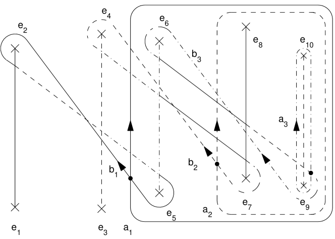
Figure 1. Basis of cycles of the curve $X$ of genus $3$. The solid, dashed and dash-dotted lines denote paths on the first, second and third sheets respectively. Correspondingly the solid to dashed line, dashed to dot-dashed line, and dot-dashed to solid lines illustrate trajectories passing through these cuts. The cuts are similarly encoded for clarity.

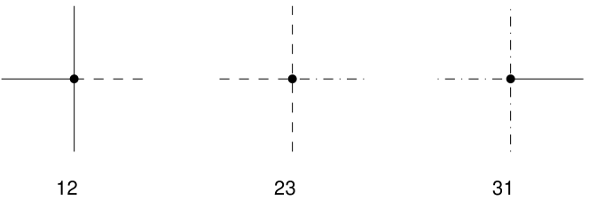
Figure 2. Contours passing from sheet 1 to sheet 2, from sheet 2 to sheet 3 and from sheet 3 to sheet 1

4. Differentials and Integrals

4.1. Holomorphic differentials and integrals

Let $X$ be algebraic curve (3.5) of genus $g$ and let $d\boldsymbol{u}(Q)=(du_{1}(Q),\ldots,du_{g}(Q))^{T}$ be the set of canonical holomorphic differentials, which are given at $n>2$ explicitly as

(4.1) $$\begin{split}du_{j}(Q)&=\frac{\,\mathrm{i}\,z^{j-1}}{\frac{\partial}{\partial w}f(z,w)}dz,\quad j=1,\ldots,n-2,\\ du_{j}(Q)&=\frac{z^{2n-3-j}\left(w-\frac{\,\mathrm{i}\,}{2}(2z)^{n}\right)}{\frac{\partial}{\partial w}f(z,w)}\,dz,\quad j=n-1,\ldots,2n-3,\end{split}$$

where $f(z,w)$ be the polynomial defining the curve (3.5). At $n=2$ the curve is elliptic; this case is studied in detail in Section 6.

If $du=\phi(z,w)dz$ is an Abelian differential, then the action of the involution $\sigma$, $\sigma^{\ast}$ say, is defined by the relation

$$\sigma^{\ast}du=\phi(\bar{z},-\bar{w})\overline{dz}.$$

For the differentials $du_{j}$ we have that

(4.2) $$\sigma^{\ast}du_{j}=-\overline{du_{j}}.$$

Introduce the matrix of $\mathfrak{a}$-periods,

$$A=\left(\oint\limits_{\mathfrak{a}_{j}}du_{k}\right)_{j,k=1,\ldots,g}.$$

From the properties (3.19) and (4.2) of $\sigma^{\ast}$ it follows that all elements of the matrix $A$ are real. Normalized form of the above differential is introduced as

(4.3) $$dv_{j}=\sum_{l=1}^{g}C_{jl}du_{l},$$

where the matrix $C=A^{-1}$. Evidently,

(4.4) $$\overline{dv_{j}}=-\sigma^{\ast}dv_{j}.$$

Now introduce $\tau$-matrix, as a matrix of $\mathfrak{b}$-periods of normalized differentials,

(4.5) $$\tau=\left(\oint\limits_{\mathfrak{b}_{j}}dv_{k}\right)_{j,k=1,\ldots,g}.$$

Then using (3.19) and (4.4) we find

$$\overline{\tau_{jk}} =\oint\limits_{\mathfrak{b}_{j}}\overline{dv}_{k}=-\oint\limits_{\mathfrak{b}_{j}}\sigma^{\ast}dv_{k}=-\oint\limits_{\sigma(\mathfrak{b}_{j})}dv_{k}$$

$$=-\tau_{jk}+2\delta_{jk}+\sum_{l\neq j}\delta_{lk}.$$

In other words we have

(4.6) $$\overline{\tau}=-\tau+\tau_{0},$$

where all diagonal elements of $\tau_{0}$ are 2 and all off-diagonal elements are 1.

4.2. Meromorphic differentials and integrals

Our construction is based on the existence of certain Abelian integrals $\Omega_{1}(Q)$ and $\Omega_{2}(Q)$ of the second kind, and similar integrals $h_{2}(Q)$ and $h_{3}(Q)$ of the third kind. We shall define these integrals as follows:

Definition 4.1.

Define normalized Abelian integrals $\Omega_{1}(Q)$ and $\Omega_{2}(Q)$ of the second kind

(4.7) $$\oint_{{\mathfrak{a}}_{j}}d\Omega_{1}=0,\quad\oint_{{\mathfrak{a}}_{j}}d\Omega_{2}=0,\quad j=1,\ldots,g,$$

where $d\Omega_{1}(Q)$, $d\Omega_{2}(Q)$, are the second kind Abelian differentials in such a way that integrals $\Omega_{1}(Q)$, and $\Omega_{2}(Q)$, have poles at the infinities $\infty_{1}$, $\infty_{2}$, $\infty_{3}$ in the vicinity of which the following expansions are valid

(4.8) $$\Omega_{1}(Q) =\begin{cases}-\,\mathrm{i}\,z+\frac{1}{2}(E_{1}+E_{2})+O\left(\frac{1}{z}\right)&\text{at}\quad Q\longrightarrow\;\infty_{1},\\ \,\mathrm{i}\,z+\frac{1}{2}(E_{2}-E_{1})+O\left(\frac{1}{z}\right)&\text{at}\quad Q\longrightarrow\;\infty_{2}\\ \,\mathrm{i}\,z-\frac{1}{2}(E_{2}-E_{1})+O\left(\frac{1}{z}\right)&\text{at}\quad Q\longrightarrow\;\infty_{3};\end{cases}$$

and

(4.9) $$\Omega_{2}(Q) =\begin{cases}-2\,\mathrm{i}\,z^{2}-\frac{1}{2}(N_{1}+N_{2})&\text{at}\quad Q\longrightarrow\;\infty_{1},\\ 2\,\mathrm{i}\,z^{2}-\frac{1}{2}(N_{2}-N_{1})&\text{at}\quad Q\longrightarrow\;\infty_{2},\\ 2\,\mathrm{i}\,z^{2}+\frac{1}{2}(N_{2}-N_{1})&\text{at}\quad Q\longrightarrow\;\infty_{3},\end{cases}$$

where $E_{1},E_{2}$ and $N_{1},N_{2}$ are certain constants.

We now compute $\mathfrak{b}$-periods for the second kind differentials. Let $P$ be a point in the vicinity of $\infty_{i}$ and $\xi$ be the local coordinate. Then the expansion of the vector of normalized holomorphic integrals reads

(4.10) $$\left.\int\limits_{Q}^{P}d\boldsymbol{v}\right|_{P\to\infty_{i}}=\boldsymbol{U}_{i}+\boldsymbol{V}^{(i)}\xi+\boldsymbol{W}^{(i)}\xi^{2}+\boldsymbol{Z}^{(i)}\xi^{3}+\ldots,\quad i=1,2,3,$$

where $\boldsymbol{U}_{i}$ are constant vectors depending on the initial point $Q$ and $\infty_{i}$,

$$\boldsymbol{U}_{i}=\int\limits_{Q}^{\infty_{i}}d\boldsymbol{v}.$$

It follows from the Bilinear Riemann Relation written for the differentials $d\Omega_{1},dv_{j}$ and $d\Omega_{2},dv_{j}$, that

(4.11) $$\boldsymbol{V} =\,\mathrm{i}\,\boldsymbol{V}^{(1)}-\,\mathrm{i}\,\boldsymbol{V}^{(2)}-\,\mathrm{i}\,\boldsymbol{V}^{(3)},$$

(4.12) $$\boldsymbol{W} =4\,\mathrm{i}\,\boldsymbol{W}^{(1)}-4\,\mathrm{i}\,\boldsymbol{W}^{(2)}-4\,\mathrm{i}\,\boldsymbol{W}^{(3)},$$

where the vectors $\boldsymbol{V}$ and $\boldsymbol{W}$ are defined as

(4.13) $$V_{j} =\frac{1}{2\,\mathrm{i}\,\pi}\oint\limits_{\mathfrak{b}_{j}}d\Omega_{1}(Q),\quad W_{j}=\frac{1}{2\,\mathrm{i}\,\pi}\oint\limits_{\mathfrak{b}_{j}}d\Omega_{2}(Q),\quad j=1,\ldots,g.$$

We shall refer below to the winding vectors $\boldsymbol{V}$ and $\boldsymbol{W}$ as the main winding vectors while the vectors $\boldsymbol{V}^{(i)}$ and $\boldsymbol{W}^{(i)}$, $i=1,2,3$ we shall call auxiliary winding vectors.

It is easy to see that the differentials $d\Omega_{1}$ and $d\Omega_{2}$ satisfy the same symmetry property (4.4) as the differentials $dv_{k}$. Hence, similar to the derivation of (4.6), we arrive to the relations

(4.14) $$\overline{V_{j}}=V_{j},\quad\overline{W_{j}}=W_{j},...,j=1,...,g.$$

Moreover, we claim that

(4.15) $$\overline{E_{k}}=-E_{k},\quad\overline{N_{k}}=-N_{k},...,k=1,2.$$

To prove the symmetry properties (4.15) let us notice that the constants $E_{1,2}$ and $N_{1,2}$ can be determined via the asymptotic relations,

(4.16) $$\int_{Q_{2}}^{Q_{1}}d\Omega_{1}=-2\,\mathrm{i}\,z+E_{1}+O\left(\frac{1}{z}\right),\quad z\to\infty,$$

(4.17) $$\int_{Q_{3}}^{Q_{1}}d\Omega_{1}=-2\,\mathrm{i}\,z+E_{2}+O\left(\frac{1}{z}\right),\quad z\to\infty,$$

(4.18) $$\int_{Q_{2}}^{Q_{1}}d\Omega_{2}=-4\,\mathrm{i}\,z^{2}-N_{1}+O\left(\frac{1}{z}\right),\quad z\to\infty,$$

(4.19) $$\int_{Q_{3}}^{Q_{1}}d\Omega_{2}=-4\,\mathrm{i}\,z^{2}-N_{2}+O\left(\frac{1}{z}\right),\quad z\to\infty,$$

where the point $Q_{j}$ belongs to the $j$-th sheet of the Riemann surface $X$,

$$\quad\pi(Q_{1})=\pi(Q_{2})=\pi(Q_{3})=z,$$

and $\pi:X\to{\mathbb{C}}$ is the canonical covering map. We assume that $z$ is a large real positive number and that the contours of integration in the integrals $\int_{Q_{2}}^{Q_{1}}$ and $\int_{Q_{3}}^{Q_{1}}$ do not intersect the basic cycles and do not pass through the points $\infty_{j}$. We shall denote these contours $\mathfrak{l}_{2}$ and $\mathfrak{l}_{3}$, respectively. The involution $\sigma$ acts on the contours $\mathfrak{l}_{j}$ as follows,

(4.20) $$\sigma(\mathfrak{l}_{2})=\mathfrak{l}_{2}+\sum_{\nu=1}^{g}n^{(2)}_{\nu}\mathfrak{a}_{\nu}+m^{(2)}\alpha_{1}+n^{(2)}\alpha_{2}+k^{(2)}\alpha_{3},$$

(4.21) $$\sigma(\mathfrak{l}_{3})=\mathfrak{l}_{3}+\sum_{\nu=1}^{g}n^{(3)}_{\nu}\mathfrak{a}_{\nu}+m^{(3)}\alpha_{1}+n^{(3)}\alpha_{3}+k^{(3)}\alpha_{2},$$

where $\alpha_{j}$ denotes a positively oriented circle around the point $\infty_{j}$ and $m^{(2,3)}$, $n^{(2,3)}$, $k^{(2,3)}$, and $n_{\nu}^{(2,3)}$ are integers. It should be also noticed, although we won’t use it right now, that the integers $m^{(2,3)}$ and $n^{(2,3)}$ have the property,

(4.22) $$m^{(j)}-n^{(j)}=\mbox{odd number},\quad j=2,3.$$

From (4.20) and (4.21) we obtain that

$$\overline{\int_{Q_{j}}^{Q_{1}}d\Omega_{k}}=\oint_{\mathfrak{l}_{j}}\overline{d\Omega_{k}}=-\oint_{\mathfrak{l}_{j}}\sigma^{*}d\Omega_{k}=-\oint_{\sigma(\mathfrak{l}_{j})}d\Omega_{k}$$

$$=-\oint_{\mathfrak{l}_{j}}d\Omega_{k}=-\int_{Q_{j}}^{Q_{1}}d\Omega_{k},\quad j=2,3,\quad k=1,2,$$

and (4.15) follows in virtue of the asymptotic (4.16) - (4.19).

Definition 4.2.

Define normalized Abelian integrals $h_{2}(Q)$ and $h_{3}(Q)$ of the third kind

(4.23) $$\oint_{{\mathfrak{a}}_{j}}dh_{2}=0,\quad\oint_{{\mathfrak{a}}_{j}}dh_{3}=0,\quad j=1,\ldots,g.$$

The integral $h_{2}(Q)$ has logarithmic singularities only and only at infinities on the first and second sheets, $\infty_{1,2}$ where it behaves locally as

(4.24) $$h_{2}(Q) =\begin{cases}\mathrm{ln}\,z-\mathrm{ln}\delta_{2}+o(1)&\text{at}\quad Q\longrightarrow\infty_{2},\\ -\mathrm{ln}\,z+\mathrm{ln}\delta_{2}+o(1)&\text{at}\quad Q\longrightarrow\infty_{1}.\end{cases}$$

The integral $h_{3}(Q)$ has logarithmic singularities only and only at infinities on the first and third sheets, $\infty_{1,3}$ where it behaves locally as

(4.25) $$h_{3}(Q) =\begin{cases}\mathrm{ln}\,z-\mathrm{ln}\delta_{3}+o(1)&\text{at}\quad Q\longrightarrow\infty_{3},\\ -\mathrm{ln}\,z+\mathrm{ln}\delta_{3}+o(1)&\text{at}\quad Q\longrightarrow\infty_{1}.\end{cases}$$

In (4.24) and (4.25) $\delta_{2}$ and $\delta_{3}$ are certain constants.

Observe that the $\mathfrak{b}$-periods of integrals $h_{2}(Q),h_{3}(Q)$ are given as

$$\frac{1}{2\pi\,\mathrm{i}\,}\oint_{{\mathfrak{b}}_{j}}dh_{2}=\int\limits_{\infty_{2}}^{\infty_{1}}dv_{j},\qquad\frac{1}{2\pi\,\mathrm{i}\,}\oint_{{\mathfrak{b}}_{j}}dh_{3}=\int\limits_{\infty_{3}}^{\infty_{1}}dv_{j},\quad j=1,\ldots,g.$$

Denote these periods as $-\boldsymbol{r}_{2,3}$, so that

(4.26) $$\int\limits_{\infty_{1}}^{\infty_{2,3}}d\boldsymbol{v}=\boldsymbol{r}_{2,3}.$$

Taking into account that $\sigma(\infty_{j})=\infty_{j}$ (cf. (3.17)) and, once again, (4.4), we conclude that

(4.27) $$\overline{\boldsymbol{r}_{2,3}}=-\boldsymbol{r}_{2,3}\quad\mbox{mod}\,\,{\mathbb{Z}}.$$

The $\sigma$ - invariance of the leading terms of the asymptotic of the differentials $dh_{2}$, $dh_{3}$ at the points $\infty_{k}$ (cf. (4.24) and (4.25)) implies, instead of (4.4), the symmetry equations,

(4.28) $$\sigma^{*}dh_{2,3}=\overline{dh_{2,3}}.$$

Similar to (4.16) - (4.19), the constant terms in the asymptotic (4.24) - (4.25) can be determined with the help of the relations

(4.29) $$\int_{Q_{k}}^{Q_{1}}dh_{k}\equiv\oint_{\mathfrak{l}_{k}}dh_{k}-2\ln z+2\ln\delta_{k}+O\left(\frac{1}{z}\right),$$

$$z\to+\infty,\quad k=2,3.$$

Similar to the case of the integrals $\Omega_{1,2}$, we can now use the symmetry properties (4.20), (4.21), and (4.28) to see that

(4.30) $$\overline{\delta_{2,3}}=-\delta_{2,3}\,.$$

Indeed, for $k=2,3$ we have

$$\overline{\oint_{\mathfrak{l}_{k}}dh_{k}}=\oint_{\mathfrak{l}_{k}}\overline{dh_{k}}=\oint_{\mathfrak{l}_{k}}\sigma^{*}dh_{k}$$

$$=\oint_{\sigma(\mathfrak{l}_{k})}dh_{k}=\oint_{\mathfrak{l}_{k}}dh_{k}+2\pi\,\mathrm{i}\,m^{(k)}\mbox{res}|_{\infty_{1}}dh_{k}+2\pi\,\mathrm{i}\,n^{(k)}\mbox{res}|_{\infty_{k}}dh_{k}$$

$$=\oint_{\mathfrak{l}_{k}}dh_{k}+2\pi\,\mathrm{i}\,(m^{(k)}-n^{(k)}),$$

and (4.30) follows in virtue of the asymptotic relation (4.29) and the parity relation (4.22 ) ( equation (4.22) is now important - it is responsible for the minus sign in (4.30)).

In the next section we shall construct explicitly the integrals $\Omega_{1,2}(P)$ and $h_{2,3}(P)$ and compute the constants $E_{1,2},N_{1,2},\delta_{2,3}$ in terms of $\theta$-functions of the curve $X$.

4.3. $\theta$-function and prime-form

The $\theta$-function of the curve $X$ with characteristic $[\varepsilon]$

$$[\varepsilon]=\left[\begin{array}[]{c}{\boldsymbol{\varepsilon}^{\prime}}^{T}\\ \boldsymbol{\varepsilon}^{T}\end{array}\right]=\left[\begin{array}[]{ccc}\varepsilon_{1}^{\prime}&\ldots&\varepsilon_{g}^{\prime}\\ \varepsilon_{1}&\ldots&\varepsilon_{g}\end{array}\right]$$

is given by the formula

(4.31) $$\theta[\varepsilon](\boldsymbol{v}) =\sum_{{\boldsymbol{n}}\in{\mathbb{Z}}^{g}}\mathrm{exp}\left\{\,\mathrm{i}\,\pi(\boldsymbol{n}+\boldsymbol{\varepsilon}^{\prime})^{T}\tau(\boldsymbol{n}+\boldsymbol{\varepsilon}^{\prime})+2\,\mathrm{i}\,\pi(\boldsymbol{n}+\boldsymbol{\varepsilon}^{\prime})^{T}(\boldsymbol{v}+\boldsymbol{\varepsilon})\right\}.$$

In this paper we are considering only half-integer characteristics, $\varepsilon_{k}^{\prime},\varepsilon_{l}=0$ or $\frac{1}{2}$ for any $k,l=1,\ldots,g$. Even characteristic $[\varepsilon]$ ($e^{4i\pi\boldsymbol{\varepsilon}^{T}\boldsymbol{\varepsilon}^{\prime}}=1$) is nonsingular if $\theta[\varepsilon](\boldsymbol{0})\neq 0$. Odd characteristic ($e^{4i\pi\boldsymbol{\varepsilon}^{T}\boldsymbol{\varepsilon}^{\prime}}=-1$) is nonsingular if the gradient $\nabla\theta[\varepsilon](\boldsymbol{0})=(\frac{\partial}{\partial v_{1}}\theta[\varepsilon](\boldsymbol{v})\big{|}_{\boldsymbol{v}=0},\ldots,\frac{\partial}{\partial v_{g}}\theta[\varepsilon](\boldsymbol{v})\big{|}_{\boldsymbol{v}=0})^{T}$ is non-zero.

The canonical $\theta$-function is the $\theta$-function with zero characteristic

(4.32) $$\theta(\boldsymbol{v})=\sum_{{\boldsymbol{n}}\in{\mathbb{Z}}^{g}}\mathrm{exp}\left\{\,\mathrm{i}\,\pi\boldsymbol{n}^{T}\tau\boldsymbol{n}+2\,\mathrm{i}\,\pi\boldsymbol{n}^{T}\boldsymbol{v}\right\}.$$

The $\theta$-function with a characteristic $[\varepsilon]$ possesses the periodicity property:

(4.33) $$\begin{split}\theta[\varepsilon](\boldsymbol{v}+\boldsymbol{e}_{k})&=\mathrm{exp}\{-2\,\mathrm{i}\,\pi\varepsilon^{\prime}_{k}\}\theta[\varepsilon](\boldsymbol{v}),\\ \theta[\varepsilon](\boldsymbol{v}+\boldsymbol{\tau}_{k})&=\mathrm{exp}\{-\,\mathrm{i}\,\pi\tau_{kk}-2\,\mathrm{i}\,\pi v_{k}-2\,\mathrm{i}\,\pi\varepsilon_{k}\}\theta[\varepsilon](\boldsymbol{v}),\end{split}$$

where $\boldsymbol{e}_{k}=(0,\ldots,1,\ldots,0)^{T}$, $\boldsymbol{\tau}_{k}=(\tau_{1k},\ldots,\tau_{gk})^{T}$ and $k=1,\ldots,g$. Using the relationship between $\overline{\tau}$ and $\tau$ derived above (see (4.6)) and definition of the $\theta$-function, we have that

(4.34) $$\overline{\theta[\varepsilon](\boldsymbol{v})}e^{-\,\mathrm{i}\,\pi{\boldsymbol{\varepsilon}^{\prime}}^{T}\tau_{0}\boldsymbol{\varepsilon}^{\prime}}\theta[\varepsilon](\overline{\boldsymbol{v}}),$$

and for the canonical $\theta$ - function,

(4.35) $$\overline{\theta(\boldsymbol{v})}=\theta(\overline{\boldsymbol{v}}).$$

The Schottky-Klein prime form [Bak95, Fay73] is defined everywhere on $X\times X$ and is introduced by the formula

(4.36) $${\mathcal{E}}(P,Q)=\frac{\theta[\varepsilon]\left(\int\limits_{Q}^{P}d\boldsymbol{v}\right)}{\sqrt{\sum_{k=1}^{g}\frac{\partial\theta[\varepsilon](\boldsymbol{0})}{\partial v_{k}}dv_{k}(P)}\sqrt{\sum_{k=1}^{g}\frac{\partial\theta[\varepsilon](\boldsymbol{0})}{\partial v_{k}}dv_{k}(Q)}},$$

where $P=(x,y)\in X$ and $Q=(z,w)\in X$ are arbitrary points and $\theta[\varepsilon](\boldsymbol{v})$ is the $\theta$-function, with non-singular odd half-integer characteristic $[\varepsilon]$. Concerning the characteristic $[\varepsilon]$ it is natural to suppose without loosing generality that the vector

$$\boldsymbol{e}=\boldsymbol{\varepsilon}+\tau\boldsymbol{\varepsilon}^{\prime}\in(\theta)\subset\mathrm{Jac}(X),\quad\theta(\boldsymbol{e})=0,$$

where $(\theta)$ be $\theta$-divisor, is parametrized as

(4.37) $$\boldsymbol{e}=\sum_{k=1}^{g-1}\int\limits_{P}^{P_{k}}d\boldsymbol{v}-\boldsymbol{K}_{P},$$

where $\boldsymbol{K}_{P}$ is vector of Riemann constants with base point $P$ and points $P_{1},\ldots,P_{g-1}$ are different branch points of the curve $X$.

The prime-form ${\mathcal{E}}(P,Q)$ vanishes only on the diagonal, $P=Q$, in the vicinity of which it is expanded in power series as

(4.38) $${\mathcal{E}}(P,Q)\sqrt{d\xi(P)d\xi(Q)}=\xi(P)-\xi(Q)+O(\xi(P)-\xi(Q)),$$

where $\xi(P)$ and $\xi(Q)$ are local coordinates of the points $P$ and $Q$ around $P_{0}$, $\xi(P_{0})=0$.

The prime-form (4.36) permits to construct symmetric second kind differential 2-differential which is called Bergmann kernel on $X\times X$ as

(4.39) $$d\omega(P,Q)= \frac{\partial^{2}}{\partial x\partial z}\;\mathrm{ln}\,{\mathcal{E}}(P,Q)\,dxdz$$

$$=\frac{\partial^{2}}{\partial x\partial z}\;\mathrm{ln}\,\theta[\varepsilon]\left(\int\limits_{Q}^{P}d\boldsymbol{v}\right)\,dxdz,$$

where $[\varepsilon]$ are non-singular odd half-integer characteristics.

The differential $d\omega(P,Q)$, where the coordinates $P,Q$ are given as $P=(x,y)$, $Q=(z,w)$ has the properties:

i) It is symmetric, $d\omega(P,Q)=d\omega(Q,P)$.

ii) It is holomorphic except on the diagonal set ($P=Q$) where it has a double pole. If the points $P,Q$ are places in the vicinity of the point $P_{0}$ and $\xi$ is the local coordinate around $P_{0}$, $\xi(P_{0})=0$ then the expansion of $d\omega(P,Q)$ near $P_{0}$ takes the form

(4.40) $$d\omega(P,Q)=\left(\frac{1}{(\xi(P)-\xi(Q))^{2}}+\frac{1}{6}S(P_{0})+O(\xi(P)-\xi(Q))\right)d\xi(P)d\xi(Q),$$

where $S(P_{0})$ holomorphic projective connection (explicit expression in terms of $\theta$-functions is given e.g. in [Fay73]).

iii) The $\mathfrak{a}$-periods taken in variable $P$ or $Q$ vanish,

(4.41) $$\oint\limits_{\mathfrak{a}_{i}}d\omega(P,Q)=0,\quad i=1,\ldots,g.$$

Introduce following notations for the directional derivatives:

$$\partial_{\boldsymbol{V}}f(\boldsymbol{v})= \sum_{k=1}^{g}V_{k}\frac{\partial}{\partial v_{k}}f(\boldsymbol{v}),$$

$$\partial^{2}_{\boldsymbol{V},\boldsymbol{W}}f(\boldsymbol{v}) \sum_{k=1}^{g}\sum_{l=1}^{g}V_{k}W_{l}\frac{\partial^{2}}{\partial v_{k}\partial v_{l}}f(\boldsymbol{v}),\;\text{etc.},$$

where $\boldsymbol{V}=(V_{1},\ldots,V_{g})^{T}$, $\boldsymbol{W}=(W_{1},\ldots,W_{g})^{T}$ are constant vectors and $f(\boldsymbol{v})$ is a function of the vector argument $\boldsymbol{v}=(v_{1},\ldots,v_{g})^{T}$. The following theorem can be found in [Fay73],[Jor92] concerning directional derivatives along the $\theta$-divisor.

Theorem 4.1.

For any nonzero vectors $\boldsymbol{a}=(a_{1},\ldots,a_{g})^{T}$, $\boldsymbol{b}=(b_{1},\ldots,b_{g})^{T}\in\mathbb{C}^{g}$ and points $P_{1},\ldots,P_{g-1}$ on $X$ the following identity holds

(4.42) $$\frac{\sum\limits_{j=1}^{g}\frac{\partial\theta}{\partial v_{j}}(\boldsymbol{e})a_{j}}{\sum\limits_{j=1}^{g}\frac{\partial\theta}{\partial v_{j}}(\boldsymbol{e})b_{j}}=\frac{\mathrm{det}\left[\boldsymbol{a}|{d}\boldsymbol{v}(P_{1})|\ldots|{d}\boldsymbol{v}(P_{g-1})\right]}{\mathrm{det}\left[\boldsymbol{b}|{d}\boldsymbol{v}(P_{1})|\ldots|{d}\boldsymbol{v}(P_{g-1})\right]},$$

where the point $\boldsymbol{e}$ is given by

(4.43) $$\boldsymbol{e}=\sum_{k=1}^{g-1}\int\limits_{P}^{P_{k}}\mathrm{d\boldsymbol{v}}-\boldsymbol{K}_{P}$$

and the matrices in (4.42) have been expressed by indicating each of $g$ columns.

Lemma 4.2.

Let $[\varepsilon]$ be non-singular odd half-integer characteristic of the curve $X$. Then

(4.44) $$\theta[\varepsilon]\left(\int\limits_{\infty_{i}}^{\infty_{j}}d\boldsymbol{v}\right)\neq 0,\quad i\neq j=1,2,3,$$

(4.45) $$\partial_{\boldsymbol{V}^{(i)}}\theta[\varepsilon](\boldsymbol{0})\neq 0,\quad i=1,2,3.$$

Proof.

The holomorphic differential $\mathrm{d}u_{1}=\,\mathrm{i}\,\mathrm{d}z/f_{w}$ vanishes at $\infty_{i}$, $i=1,2,3$ to the order $4n-8=2g-2$ and therefore $(2g-2)\infty_{i}$ is equivalent to the canonical class. Hence the vector of Riemann constants with the base point at $\infty_{i}$ is a half-period [FK80]. The curve considered has only simple branch points (see the proof of Lemma 3.1) and therefore non-singular odd half-period corresponding to the characteristic $[\varepsilon]$ can be given by the formula (4.43) with $P_{i}$, $i=1,\ldots$ being branch points.

First prove (4.45) for $i=1$, $j=2$. Suppose the opposite. Then the vanishing of the directional derivative $\partial_{\boldsymbol{V}^{(2)}}\theta(\boldsymbol{0})=0$ will lead, according to (4.42), to the vanishing of the determinant

$$\mathrm{det}\left[\boldsymbol{V}^{(2)}|{d}\boldsymbol{v}(P_{1})|\ldots|{d}\boldsymbol{v}(P_{g-1})\right]=\mathrm{det}\left[\left.\left.\left.\frac{{d}\boldsymbol{v}(\infty_{2})}{d\xi(\infty_{2})}\right|{d}\boldsymbol{v}(P_{1})\right|\ldots\right|{d}\boldsymbol{v}(P_{g-1})\right]$$

But there is no $\infty_{2}$ among branch points $P_{i}$ as that was shown earlier. The contradiction obtained proves the statement. Other cases are considered analogously.

Prove (4.44). Suppose the opposite. Consider further the prime-form $\mathcal{E}(P,\infty_{1})$ given by the formula (4.36). It is well defined because directional derivative $\partial_{\boldsymbol{V}^{(1)}}\theta(\boldsymbol{0})\neq 0$. According to principal property of the prime-form it vanishes only at $P=\infty_{1}$. Therefore the supposed vanishing of the $\theta$-function should lead to vanishing of the directional derivative in the denominator. The contradiction obtained proves the statement. ∎

4.4. $\theta$-functional construction of meromorphic integrals

To construct the required second and third kind integrals $\Omega_{1,2}(Q)$ and $h_{2,3}(Q)$ we first construct corresponding meromorphic differentials with the aid of prime-form introduced.

The normalized meromophic differential of the third kind, $dh_{2}$ with the poles in $\infty_{1}$ and $\infty_{2}$ of the first order and residues $\pm 1$ in the poles is given as

(4.46) $$dh_{2}(P)=d_{z}\,\mathrm{ln}\,\frac{{\mathcal{E}}(P,\infty_{1})}{{\mathcal{E}}(P,\infty_{2})}.$$

Analogously the normalized meromophic differential of the third kind, $dh_{3}$ with the poles in $\infty_{1}$ and $\infty_{3}$ the first order and residues $\pm 1$ in the poles is given as

(4.47) $$dh_{3}(P)=d_{z}\,\mathrm{ln}\,\frac{{\mathcal{E}}(P,\infty_{1})}{{\mathcal{E}}(P,\infty_{3})}.$$

We are in position now to give $\theta$-functional representation for the second and third kind integrals, which permit us to compute 6 constants $E_{1,2}$, $N_{1,2}$ and $\delta_{2,3}$ in terms of $\theta$-functions.

Consider three quantities

(4.48) $$\begin{split}\Omega^{(i)}_{1}(P)&=\left.\int dx\left\{\frac{\partial}{\partial x\partial z}\mathrm{ln}\,\theta[\varepsilon]\left(\int\limits_{Q}^{P}d\boldsymbol{v}\right)dz\right\}\right|_{Q=\infty_{i}}\frac{1}{d\xi(\infty_{i})}\\ &=\left.\sum_{k=1}^{g}V_{k}^{(i)}\frac{\partial}{\partial v_{k}}\,\mathrm{ln}\,\theta[\varepsilon](\boldsymbol{v})\right|_{\boldsymbol{v}=\int\limits_{\infty_{i}}^{P}d\boldsymbol{v}}\\ &=\partial_{\boldsymbol{V}^{(i)}}\,\mathrm{ln}\,\theta[\varepsilon]\left(\int\limits_{\infty_{i}}^{P}d\boldsymbol{v}\right),\end{split}$$

where $i=1,2,3$ and the point $Q$ has coordinates $(z,w)$.

Lemma 4.3.

The quantities $\Omega^{(i)}_{1}(P)$, $i=1,2,3$ are second kind Abelian integrals with unique pole of the first order at corresponding to the index $i$ infinity $\infty_{i}$ with $\boldsymbol{\mathfrak{a}}$ and $\boldsymbol{\mathfrak{b}}$-periods,

(4.49) $$\oint\limits_{\mathfrak{a}_{l}}d\Omega^{(i)}_{1}(P)=0,\quad\oint\limits_{\mathfrak{b}_{l}}d\Omega^{(i)}_{1}(P)=-2\,\mathrm{i}\,\pi V_{l}^{(i)}\quad l=1,\ldots,g$$

and following behaviour at the infinities $\infty_{1},\infty_{2},\infty_{3}$ on different sheets

(4.50) $$\begin{split}\Omega_{1}^{(1)}(P)&=\begin{cases}\frac{1}{\xi}+c_{1}^{(1)}+O(\xi),\\ X_{1,2}+O(\xi),\\ X_{1,3}+O(\xi),\end{cases}\qquad\Omega_{1}^{(2)}(P)=\begin{cases}X_{2,1}+O(\xi),\\ \frac{1}{\xi}+c_{1}^{(2)}+O(\xi),\\ X_{2,3}+O(\xi),\end{cases}\\ \Omega_{1}^{(3)}(P)&=\begin{cases}X_{3,1}+O(\xi),\\ X_{3,2}+O(\xi),\\ \frac{1}{\xi}+c_{1}^{(3)}+O(\xi),\end{cases}\end{split}$$

where

(4.51) $$X_{i,j} =\partial_{\boldsymbol{V}^{(i)}}\mathrm{ln}\theta[\varepsilon]\left(\int\limits_{\infty_{i}}^{\infty_{j}}d\boldsymbol{v}\right),\quad i\neq j=1,2,3,$$

(4.52) $$c_{1}^{(i)} =\frac{1}{2}\frac{\partial^{2}_{\boldsymbol{V}^{(i)},\boldsymbol{V}^{(i)}}\theta[\varepsilon](\boldsymbol{0})}{\partial_{\boldsymbol{V}^{(i)}}\theta[\varepsilon](\boldsymbol{0})}-\frac{\partial_{\boldsymbol{W}^{(i)}}\theta[\varepsilon](\boldsymbol{0})}{\partial_{\boldsymbol{V}^{(i)}}\theta[\varepsilon](\boldsymbol{0})},\quad i=1,2,3.$$

Proof.

Relations (4.49) for periods follow immediately from definition and periodicity properties (4.33) of the $\theta$-function, while expansions (4.50) result direct computation. The quantities (4.51) and (4.52) are well defined because of inequalities (4.44) and (4.45). ∎

Similar statement is valid for three quantities

(4.53) $$\Omega^{(i)}_{2}(P)=\left(2\partial_{\boldsymbol{W}^{(i)}}-\partial^{2}_{\boldsymbol{V}^{(i)},\boldsymbol{V}^{(i)}}\right)\mathrm{ln}\,\theta[\varepsilon]\left(\int\limits_{\infty_{i}}^{P}d\boldsymbol{v}\right),$$

where $i=1,2,3$ and the point $Q$ has coordinates $(z,w)$.

Lemma 4.4.

The quantities $\Omega^{(i)}_{2}(P)$, $i=1,2,3$ are second kind Abelian integrals with unique pole of second order at corresponding to the index $i$ infinity $\infty_{i}$ with $\boldsymbol{\mathfrak{a}}$ and $\boldsymbol{\mathfrak{b}}$-periods,

(4.54) $$\int\limits_{\mathfrak{a}_{l}}d\Omega^{(i)}_{2}(P)=0,\quad\int\limits_{\mathfrak{b}_{l}}d\Omega^{(i)}_{2}(P)=-4\,\mathrm{i}\,\pi W_{l}^{(i)}\quad l=1,\ldots,g$$

and following behavior at the infinities on different sheets

(4.55) $$\begin{split}\Omega_{2}^{(1)}(P)&=\begin{cases}\frac{1}{\xi^{2}}+c_{2}^{(1)}+O(\xi),\\ Y_{1,2}+O(\xi),\\ Y_{1,3}+O(\xi),\end{cases}\qquad\Omega_{2}^{(2)}(P)=\begin{cases}Y_{2,1}+O(\xi),\\ \frac{1}{\xi^{2}}+c_{2}^{(2)}+O(\xi),\\ Y_{2,3}+O(\xi),\end{cases}\\ \Omega_{2}^{(3)}(P)&=\begin{cases}Y_{3,1}+O(\xi),\\ Y_{3,2}+O(\xi),\\ \frac{1}{\xi^{2}}+c_{2}^{(3)}+O(\xi),\end{cases}\end{split}$$

where

(4.56) $$Y_{i,j} =\left(2\partial_{\boldsymbol{W}^{(i)}}-\partial^{2}_{\boldsymbol{V}^{(i)},\boldsymbol{V}^{(i)}}\right)\mathrm{ln}\theta[\varepsilon]\left(\int\limits_{\infty_{i}}^{\infty_{j}}d\boldsymbol{v}\right),$$

(4.57) $$c_{2}^{(i)} =-\left(\frac{\partial_{\boldsymbol{W}^{(i)}}\theta[\varepsilon](\boldsymbol{0})}{\partial_{\boldsymbol{V}^{(i)}}\theta[\varepsilon](\boldsymbol{0})}\right)^{2}+\frac{1}{3}\frac{\partial^{3}_{\boldsymbol{V}^{(i)},\boldsymbol{V}^{(i)},\boldsymbol{V}^{(i)}}\theta[\varepsilon](\boldsymbol{0})}{\partial_{\boldsymbol{V}^{(i)}}\theta[\varepsilon](\boldsymbol{0})}+\frac{\partial_{\boldsymbol{Z}^{(i)}}\theta[\varepsilon](\boldsymbol{0})}{\partial_{\boldsymbol{V}^{(i)}}\theta[\varepsilon](\boldsymbol{0})}.$$

Proof.

The second term in (4.53) does not contribute to periods – it is meromorphic function but the first term in (4.53) leads to the relations (4.54). The expansions (4.55) result direct computation. The quantities (4.56) and (4.57) are well defined because of inequalities (4.44) and (4.45). ∎

The normalized meromorphic differential of the second kind $d\Omega_{1}(P)$ and $d\Omega_{2}(P)$ are then given as

(4.58) $$\Omega_{1}(P) =-\,\mathrm{i}\,\Omega_{1}^{(1)}(P)+\,\mathrm{i}\,\Omega_{1}^{(2)}(P)+\,\mathrm{i}\,\Omega_{1}^{(3)}(P)+C_{1},$$

(4.59) $$\Omega_{2}(P) =-2\,\mathrm{i}\,\Omega_{2}^{(1)}(P)+2\,\mathrm{i}\,\Omega_{2}^{(2)}(P)+2\,\mathrm{i}\,\Omega_{2}^{(3)}(P)+C_{2},$$

where $C_{k}$, $k=1,2$ are constants and integrals $\Omega_{i}^{(j)}(P)$ are given in (4.48) and (4.53).

The representations (4.58,4.59) of the meromorphic differentials permits to compute the constants $E_{1,2},N_{1,2}$ and $\delta_{2,3}$ in terms of $\theta$-functions

Theorem 4.5.

The following $\theta$-functional expressions are valid for the constants $E_{1,2},N_{1,2}$ and $\delta_{2,3}$:

(4.60) $$\begin{split}E_{1}&=\,\mathrm{i}\,\left(X_{12}+X_{21}+X_{31}-X_{32}-c_{1}^{(2)}-c_{1}^{(1)}\right),\\ E_{2}&=\,\mathrm{i}\,\left(X_{13}+X_{31}+X_{21}-X_{23}-c_{1}^{(3)}-c_{1}^{(1)}\right)\end{split}$$

and

(4.61) $$\begin{split}N_{1}&=-2\,\mathrm{i}\,\left(Y_{12}+Y_{21}+Y_{31}-Y_{32}-c_{2}^{(2)}-c_{2}^{(1)}\right),\\ N_{2}&=-2\,\mathrm{i}\,\left(Y_{13}+Y_{31}+Y_{21}-Y_{23}-c_{2}^{(3)}-c_{2}^{(1)}\right)\end{split}$$

and

(4.62) $$\delta_{2,3} =\frac{\,\mathrm{i}\,}{\theta[\varepsilon](\boldsymbol{r}_{2,3})}\sqrt{\partial_{\boldsymbol{V}^{(2,3)}}\theta[\varepsilon](\boldsymbol{0})}\sqrt{\partial_{\boldsymbol{V}^{(1)}}\theta[\varepsilon](\boldsymbol{0})},$$

where quantities $X_{i,j},Y_{i,j},c_{k}^{(i)}$ are defined in (4.51), (4.56), (4.52) and (4.57).

Proof.

Consider first integral with the first order poles at infinities. Expand (4.58) at $\infty_{1},\infty_{2},\infty_{3}$ and compare with the asymptotic conditions (4.8) to obtain equations

$$\,\mathrm{i}\,X_{21}+\,\mathrm{i}\,X_{31}+C_{1}-\,\mathrm{i}\,c_{1}^{(1)} =\frac{1}{2}E_{1}+\frac{1}{2}E_{2},$$

$$-\,\mathrm{i}\,X_{12}+\,\mathrm{i}\,X_{32}+C_{1}+\,\mathrm{i}\,c_{1}^{(2)} =\frac{1}{2}E_{2}-\frac{1}{2}E_{1},$$

$$-\,\mathrm{i}\,X_{13}+\,\mathrm{i}\,X_{23}+C_{1}+\,\mathrm{i}\,c_{1}^{(3)} =-\frac{1}{2}E_{2}+\frac{1}{2}E_{1}.$$

We find (4.60) and the following expression for the constant

$$C_{1} =\frac{\,\mathrm{i}\,}{2}\left(X_{12}+X_{13}\right)-\frac{\,\mathrm{i}\,}{2}\left(X_{32}+X_{23}\right)+\frac{\,\mathrm{i}\,}{2}(c_{1}^{(2)}+c_{1}^{(3)}).$$

Consider further the integral with the second order poles at infinities. Expand (4.59) at $\infty_{1},\infty_{2},\infty_{3}$ and compare with the asymptotic conditions (4.9). Solving linear equations as before we find (4.61) and the following expression for the constant

$$C_{2} =\frac{\,\mathrm{i}\,}{2}\left(Y_{12}+Y_{13}\right)-\frac{\,\mathrm{i}\,}{2}\left(Y_{32}+Y_{23}\right)+\frac{\,\mathrm{i}\,}{2}(c_{2}^{(2)}+c_{2}^{(3)}).$$

Consider further the third kind integral

(4.63) $$h_{2}(P)=\mathrm{ln}\,\frac{{\mathcal{E}}(P,\infty_{1})}{{\mathcal{E}}(P,\infty_{2})}+C_{h}.$$

On the first sheet we have that, as $P\to\infty_{1}$,

$$h_{2}(P) =\mathrm{ln}\frac{\theta[\varepsilon]\left(\int\limits_{\infty_{1}}^{P}d\boldsymbol{v}\right)}{\theta[\varepsilon]\left(\int\limits_{\infty_{2}}^{P}d\boldsymbol{v}\right)}\frac{\sqrt{\sum_{k=1}^{g}\frac{\partial\theta[\varepsilon](\boldsymbol{0})}{\partial v_{k}}dv_{k}(\infty_{2})}}{\sqrt{\sum_{k=1}^{g}\frac{\partial\theta[\varepsilon](\boldsymbol{0})}{\partial v_{k}}dv_{k}(\infty_{1})}}+C_{h}+O(\xi)$$

(4.64) $$=\mathrm{ln}\,\xi+\mathrm{ln}\sqrt{\sum_{k=1}^{g}V_{k}^{(2)}\frac{\partial}{\partial v_{k}}\,\theta[\varepsilon](\boldsymbol{0})}\sqrt{\sum_{k=1}^{g}V_{k}^{(1)}\frac{\partial}{\partial v_{k}}\,\theta[\varepsilon](\boldsymbol{0})}$$

$$-\mathrm{ln}\,\theta[\varepsilon](-\boldsymbol{r}_{2})+C_{h}+O(\xi)$$

whilst on the second sheet, as $P\to\infty_{2}$, we have

$$h_{2}(P) =-\mathrm{ln}\,\xi-\mathrm{ln}\sqrt{\sum_{k=1}^{g}V_{k}^{(2)}\frac{\partial}{\partial v_{k}}\,\theta[\varepsilon](\boldsymbol{0})}\sqrt{\sum_{k=1}^{g}V_{k}^{(1)}\frac{\partial}{\partial v_{k}}\,\theta[\varepsilon](\boldsymbol{0})}$$

(4.65) $$+\mathrm{ln}\,\theta[\varepsilon](\boldsymbol{r}_{2})+C_{h}+O(\xi).$$

Comparison of expansions (4.64) and (4.65) with the expansions (4.24) leads to $C_{h}=\frac{\,\mathrm{i}\,\pi}{2}$, and

$$\delta_{2}=\frac{\,\mathrm{i}\,}{\theta[\varepsilon](\boldsymbol{r}_{2})}\sqrt{\sum_{k=1}^{g}V_{k}^{(2)}\frac{\partial}{\partial v_{k}}\,\theta[\varepsilon](\boldsymbol{0})}\sqrt{\sum_{k=1}^{g}V_{k}^{(1)}\frac{\partial}{\partial v_{k}}\,\theta[\varepsilon](\boldsymbol{0})}.$$

The expression for $\delta_{2}$ in (4.62) follows. The expression for $\delta_{3}$ in (4.62) is derived analogously. ∎

We emphasize that the constants described in the Theorem 4.5 are fundamental: expression for the constants $c_{2}^{(i)}$ coincide with accuracy to a trivial multiplier with values of the projective connection, $S(P)$ (see (4.40)) at infinities, $S(\infty_{i}),i=1,2,3$. The quantities $X_{i,j}$ and $Y_{i,j}$ can be expressed in terms of multidimensional Kleinian $\zeta$ and $\wp$-function whose classical and modern treatment, in the hyperelliptic case, can be found in [Bak95] and [BEL97] correspondingly. We also remark that analogous expressions for constants $E_{1,2}$, $N_{1,2}$ in terms of $\theta$-functions and winding vectors for Thirring model which is associated with a hyperelliptic curve are obtained in [EGH00], see also [GH03].

The important symmetry relations for the costants $E_{1,2}$, $N_{1,2}$, and $\delta_{2,3}$, which have been derived earlier (see (4.15) and (4.30)), can be also easily obtained from the $\theta$-functional formulae of Theorem 4.5 with the help of equation (4.34).

5. Algebro-geometric solutions of the Manakov system

We now summarize a list of basic objects which are related to the curve (3.5)

1. A homology basis of oriented cycles $\mathfrak{a}_{j}$ and $\mathfrak{b}_{j}$ as discussed in the Section 3.

2. The differentials $dv_{j}$ introduced in the Section 4.1 are normalized.

3. The matrix of the $\mathfrak{b}$-periods of the trigonal curve $X$ and the associated $\theta$-functions as defined by equations (4.5) and (4.31) respectively.

4. The Abelian integrals $\Omega_{1}(Q)$, $\Omega_{2}(Q)$, $h_{1}(Q)$ and $h_{2}(Q)$, $Q\in X$ which are fixed by the conditions (4.8), (4.9) and (4.24), (4.25).

5. An arbitrary divisor $\mathcal{D}$ with degree $\mathrm{deg}{\mathcal{D}}=g$ of general position, i.e.

$$\mathcal{D}=\sum_{i=1}^{g}Q_{i},\quad\pi(Q_{i})\neq e_{i},\quad i\neq k\Rightarrow\pi(Q_{i})\neq\pi(Q_{j}),$$

where $\pi(P)$ is three sheeted covering

$$\pi:X\longrightarrow\mathbb{CP}^{1},\qquad\pi^{-1}(\infty)=(\infty_{1},\infty_{2},\infty_{3}),$$

and $e_{i}$ are the branch points of the curve $X$.

The vector valued Baker-Akhiezer function

$$\boldsymbol{\Psi}(Q,x,t)=(\psi_{1}(Q,x,t),\psi_{2}(Q,x,t),\psi_{3}(Q,x,t))^{T}$$

is uniquely defined by two conditions. The first of these conditions describes the analytic structure of $\boldsymbol{\Psi}$ on $X/\{\infty_{1,2,3}\}$

I. $\psi_{i}(Q,x,t)$, $i=1,2,3$ are meromorphic on $X/\{\infty_{1,2,3}\}$. Their divisor of poles coincides with $\mathcal{D}$.

The second condition describes the asymptotic behavior of $\boldsymbol{\Psi}(Q,x,t)$ at $\infty_{1,2,3}$ and shows that $\boldsymbol{\Psi}(Q,x,t)$ has essential singularities at $\infty_{1,2,3}$

II. As $Q\to\infty_{1,2,3}$, the asymptotic behavior of $\boldsymbol{\Psi}(Q,x,t)$ is given by the equations,

$$\boldsymbol{\Psi}(Q) = \left[\left(\begin{array}[]{c}1\\ 0\\ 0\end{array}\right)+O(z^{-1})\right]\mathrm{exp}(-\,\mathrm{i}\,zx-2\,\mathrm{i}\,z^{2}t)$$

at $$Q\longrightarrow\infty_{1},\quad z=\pi(Q),$$

$$\boldsymbol{\Psi}(Q) = \frac{z}{\delta_{2}}\left[\left(\begin{array}[]{c}0\\ 1\\ 0\end{array}\right)+O(z^{-1})\right]\mathrm{exp}(\,\mathrm{i}\,zx+2\,\mathrm{i}\,z^{2}t)$$

at $$Q\longrightarrow\infty_{2},\quad z=\pi(Q),$$

$$\boldsymbol{\Psi}(Q) = \frac{z}{\delta_{3}}\left[\left(\begin{array}[]{c}0\\ 0\\ 1\end{array}\right)+O(z^{-1})\right]\mathrm{exp}(\,\mathrm{i}\,zx+2\,\mathrm{i}\,z^{2}t)$$

at $$Q\longrightarrow\infty_{3},\quad z=\pi(Q),$$

where $\delta_{2},\delta_{3}\in\mathbb{C}$ are non-zero constants. Indeed, we shall take $\delta_{2}$ and $\delta_{3}$ from (4.24) and (4.25), respectively.

Then, $\boldsymbol{\Psi}(Q,x,t)=(\psi_{1}(Q,x,t),\psi_{2}(Q,x,t),\psi_{3}(Q,x,t))^{T}$ is uniquely determined by the conditions I. and II. and may be explicitly constructed by the formula

(5.4) $$\psi_{1}(Q) =\frac{\theta\left(\int\limits_{\infty_{1}}^{Q}d\boldsymbol{v}+\boldsymbol{\Gamma}\right)\theta(\boldsymbol{D})}{\theta\left(\int\limits_{\infty_{1}}^{Q}d\boldsymbol{v}-\boldsymbol{D}\right)\theta(\boldsymbol{\Gamma})}\mathrm{exp}\{x\Omega_{1}(Q)+t\Omega_{2}(Q)-Ex+Nt\},$$

$$\psi_{2}(Q) =\frac{\theta\left(\int\limits_{\infty_{1}}^{Q}d\boldsymbol{v}+\boldsymbol{\Gamma}-\boldsymbol{r}_{2}\right)\theta(\boldsymbol{D}-\boldsymbol{r}_{2})}{\theta\left(\int\limits_{\infty_{1}}^{Q}d\boldsymbol{v}-\boldsymbol{D}\right)\theta(\boldsymbol{\Gamma})}$$

(5.5) $$\qquad\times\mathrm{exp}\{x\Omega_{1}(Q)+t\Omega_{2}(Q)-E^{\prime}x+N^{\prime}t+h_{2}\},$$

$$\psi_{3}(Q) =\frac{\theta\left(\int\limits_{\infty_{1}}^{Q}d\boldsymbol{v}+\boldsymbol{\Gamma}-\boldsymbol{r}_{3}\right)\theta(\boldsymbol{D}-\boldsymbol{r}_{3})}{\theta\left(\int\limits_{\infty_{1}}^{Q}d\boldsymbol{v}-\boldsymbol{D}\right)\theta(\boldsymbol{\Gamma})}$$

(5.6) $$\qquad\times\mathrm{exp}\{x\Omega_{1}(Q)+t\Omega_{2}(Q)+E^{\prime}x-N^{\prime}t+h_{3}\},$$

where

(5.7) $$\boldsymbol{\Gamma}\boldsymbol{V}x+\boldsymbol{W}t-\boldsymbol{D}$$

and

(5.8) $$\boldsymbol{D}=\sum_{j=1}^{g}\int\limits_{\infty_{1}}^{Q_{j}}d\boldsymbol{v}-\boldsymbol{K}_{\infty_{1}}.$$

Here, $\boldsymbol{K}_{\infty_{1}}$ is the vector of Riemann constants with the base point $\infty_{1}$. The constants $E,E^{\prime},N,N^{\prime}$ are defined by $E=(E_{1}+E_{2})/2$, $E^{\prime}=-(E_{1}-E_{2})/2$, and $N=(N_{1}+N_{2})/2$, $N^{\prime}=-(N_{1}-N_{2})/2$, where $E_{1},E_{2},N_{1}$ and $N_{2}$ are the basic constants from (4.8) and (4.9).

The parameters appearing in the above expressions $\psi_{i}(Q,x,t)$ are defined in (4.13), and vectors $\boldsymbol{r}_{2,3}$ are defined in (4.26).

The proof of formulae (5.4,5.5,5.6) is based on the standard arguments of the theory of algebro-geometric integration: the Riemann theorem, which provides the condition I., the non-speciality of the divisor $\mathcal{D}$, which guarantee the uniqueness of the function $\boldsymbol{\Psi}(Q,x,t)$, and the periodicity properties (4.33) of the $\theta$ - function, which ensure that the equations (5.4) - (5.6) define a single-valued (meromorphic) function on $X$. (For more details - see e.g. the similar proof for the usual, one-component NLS discussed in Ch. 4 of [BBE⁺94].)

We now fix some connected neighborhood $U$ of the point $z=\infty$ on $\mathbb{C}\mathbb{P}^{1}$ which has no branch points. Then, for each $z\in U$, $\pi^{-1}(z)$ contains exactly three points denoted by $Q_{j}\in X$, $j=1,2,3$, so that $Q_{j}\to\infty_{j}$ when $z\to\infty$. For $z\in U$ the matrix function

(5.9) $$\Psi(z,x,t)=\left(\boldsymbol{\Psi}(Q_{1},x,t),\boldsymbol{\Psi}(Q_{2},x,t),\boldsymbol{\Psi}(Q_{3},x,t)\right)$$

is now correctly defined to enable us to use the [BBE⁺94] version of Krichever’s method [Kri77] to solve the VNSE. This will require the asymptotic form for $\Psi(z,x,t)$, whose leading term is

$$\left(\begin{array}[]{lllll}\mathrm{e}^{\{-ixz-2\,\mathrm{i}\,tz^{2}\}}&\begin{array}[]{l}\vdots\\ \vdots\\ \vdots\end{array}&\begin{array}[]{l}\frac{\theta(\boldsymbol{r}_{2}+\boldsymbol{\Gamma})\theta(\boldsymbol{D})}{\theta(\boldsymbol{r}_{2}-\boldsymbol{D})\theta(\boldsymbol{\Gamma})}\\ \times\mathrm{e}^{\{ixz+2\,\mathrm{i}\,tz^{2}\}}\\ \times\mathrm{e}^{\{-E_{1}x+N_{1}t\}}\end{array}&\begin{array}[]{l}\vdots\\ \vdots\\ \vdots\end{array}&\begin{array}[]{l}\frac{\theta(\boldsymbol{r}_{3}+\boldsymbol{\Gamma})\theta(\boldsymbol{D})}{\theta(\boldsymbol{r}_{3}-\boldsymbol{D})\theta(\boldsymbol{\Gamma})}\\ \times\mathrm{e}^{\{ixz+2\,\mathrm{i}\,tz^{2}\}}\\ \times\mathrm{e}^{\{-E_{2}x+N_{2}t\}}\end{array}\\ \dotfill&\dotfill&\dotfill&\dotfill&\dotfill\\ \begin{array}[]{l}\frac{\delta_{2}}{z}\frac{\theta(\boldsymbol{r}_{2}-\boldsymbol{\Gamma})\theta(\boldsymbol{D}-\boldsymbol{r}_{2})}{\theta(\boldsymbol{D})\theta(\boldsymbol{\Gamma})}\\ \times\mathrm{e}^{\{-ixz-2\,\mathrm{i}\,tz^{2}\}}\\ \times\mathrm{e}^{\{E_{1}x-N_{1}t\}}\end{array}&\begin{array}[]{l}\vdots\\ \vdots\\ \vdots\end{array}&\frac{z}{\delta_{2}}\mathrm{e}^{\{ixz+2\,\mathrm{i}\,tz^{2}\}}&\begin{array}[]{l}\vdots\\ \vdots\\ \vdots\end{array}&\begin{array}[]{l}\frac{\theta(\boldsymbol{r}_{3}-\boldsymbol{r}_{2}+\boldsymbol{\Gamma})\theta(\boldsymbol{D}-\boldsymbol{r}_{2})}{\theta(\boldsymbol{r}_{3}-\boldsymbol{D})\theta(\boldsymbol{\Gamma})}\\ \times\mathrm{e}^{\{ixz+2\,\mathrm{i}\,tz^{2}\}}\\ \times\mathrm{e}^{\{-(E_{2}-E_{1})x+(N_{2}-N_{1})t\}}\end{array}\\ \dotfill&\dotfill&\dotfill&\dotfill&\dotfill\\ \begin{array}[]{l}\frac{\delta_{3}}{z}\frac{\theta(\boldsymbol{r}_{3}-\boldsymbol{\Gamma})\theta(\boldsymbol{D}-\boldsymbol{r}_{3})}{\theta(\boldsymbol{D})\theta(\boldsymbol{\Gamma})}\\ \times\mathrm{e}^{\{-ixz-2\,\mathrm{i}\,tz^{2}\}}\\ \times\mathrm{e}^{\{E_{2}x-N_{2}t\}}\end{array}&\begin{array}[]{l}\vdots\\ \vdots\\ \vdots\end{array}&\begin{array}[]{l}\frac{\theta(\boldsymbol{r}_{2}-\boldsymbol{r}_{3}+\boldsymbol{\Gamma})\theta(\boldsymbol{D}-\boldsymbol{r}_{2})}{\theta(\boldsymbol{r}_{2}-\boldsymbol{D})\theta(\boldsymbol{\Gamma})}\\ \times\mathrm{e}^{\{ixz+2\,\mathrm{i}\,tz^{2}\}}\\ \times\mathrm{e}^{\{(E_{2}-E_{1})x-(N_{2}-N_{1})t\}}\end{array}&\begin{array}[]{l}\vdots\\ \vdots\\ \vdots\end{array}&\frac{z}{\delta_{3}}\mathrm{e}^{\{ixz+2\,\mathrm{i}\,tz^{2}\}}\end{array}\right)$$

$$= \left(\begin{array}[]{lllll}\qquad\qquad 1+O\left(\frac{1}{z}\right)&\begin{array}[]{l}\vdots\\ \vdots\\ \vdots\end{array}&\begin{array}[]{l}\frac{\delta_{2}}{z}\frac{\theta(\boldsymbol{r}_{2}+\boldsymbol{\Gamma})\theta(\boldsymbol{D})}{\theta(\boldsymbol{r}_{2}-\boldsymbol{D})\theta(\boldsymbol{\Gamma})}\\ \times\mathrm{e}^{\{-E_{1}x+N_{1}t\}}\\ +O\left(\frac{1}{z^{2}}\right)\end{array}&\begin{array}[]{l}\vdots\\ \vdots\\ \vdots\end{array}&\begin{array}[]{l}\frac{\delta_{3}}{z}\frac{\theta(\boldsymbol{r}_{3}+\boldsymbol{\Gamma})\theta(\boldsymbol{D})}{\theta(\boldsymbol{r}_{3}-\boldsymbol{D})\theta(\boldsymbol{\Gamma})}\\ \times\mathrm{e}^{\{-E_{2}x+N_{2}t\}}\\ +O\left(\frac{1}{z^{2}}\right)\end{array}\\ \dotfill&\dotfill&\dotfill&\dotfill&\dotfill\\ \begin{array}[]{l}\frac{\delta_{2}}{z}\frac{\theta(\boldsymbol{r}_{2}-\boldsymbol{\Gamma})\theta(\boldsymbol{D}-\boldsymbol{r}_{2})}{\theta(\boldsymbol{D})\theta(\boldsymbol{\Gamma})}\\ \times\mathrm{e}^{\{E_{1}x-N_{1}t\}}\\ +O\left(\frac{1}{z^{2}}\right)\end{array}&\begin{array}[]{l}\vdots\\ \vdots\\ \vdots\end{array}&\qquad\qquad 1+O\left(\frac{1}{z}\right)&\begin{array}[]{l}\vdots\\ \vdots\\ \vdots\end{array}&\begin{array}[]{l}\frac{\delta_{3}}{z}\frac{\theta(\boldsymbol{r}_{3}-\boldsymbol{r}_{2}+\boldsymbol{\Gamma})\theta(\boldsymbol{D}-\boldsymbol{r}_{2})}{\theta(\boldsymbol{r}_{3}-\boldsymbol{D})\theta(\boldsymbol{\Gamma})}\\ \times\mathrm{e}^{\{-(E_{2}-E_{1})x+(N_{2}-N_{1})t\}}\\ +O\left(\frac{1}{z^{2}}\right)\end{array}\\ \dotfill&\dotfill&\dotfill&\dotfill&\dotfill\\ \begin{array}[]{l}\frac{\delta_{3}}{z}\frac{\theta(\boldsymbol{r}_{3}-\boldsymbol{\Gamma})\theta(\boldsymbol{D}-\boldsymbol{r}_{3})}{\theta(\boldsymbol{D})\theta(\boldsymbol{\Gamma})}\\ \times\mathrm{e}^{\{E_{2}x-N_{2}t\}}\\ +O\left(\frac{1}{z^{2}}\right)\end{array}&\begin{array}[]{l}\vdots\\ \vdots\\ \vdots\end{array}&\begin{array}[]{l}\frac{\delta_{2}}{z}\frac{\theta(\boldsymbol{r}_{2}-\boldsymbol{r}_{3}+\boldsymbol{\Gamma})\theta(\boldsymbol{D}-\boldsymbol{r}_{2})}{\theta(\boldsymbol{r}_{2}-\boldsymbol{D})\theta(\boldsymbol{\Gamma})}\\ \times\mathrm{e}^{\{(E_{2}-E_{1})x-(N_{2}-N_{1})t\}}\\ +O\left(\frac{1}{z^{2}}\right)\end{array}&\begin{array}[]{l}\vdots\\ \vdots\\ \vdots\end{array}&\qquad\qquad 1+O\left(\frac{1}{z}\right)\end{array}\right)$$

$$\qquad\qquad\qquad\qquad\times\mathrm{exp}\{\,\mathrm{i}\,zxJ+2\,\mathrm{i}\,z^{2}tJ\}\left(\begin{array}[]{ccc}1&{}\hfil&{}\hfil\\ {}\hfil&\frac{z}{\delta_{2}}&{}\hfil\\ {}\hfil&{}\hfil&\frac{z}{\delta_{3}}\end{array}\right),$$

where

(5.10) $$J=\left(\begin{array}[]{cc}-1&\boldsymbol{0}^{T}\\ \boldsymbol{0}&1_{2}\end{array}\right).$$

Theorem 5.1.

Let ${\mathcal{D}}=Q_{1}+\ldots,Q_{g}$ be non-special divisor of degree $g$ satisfying the reality condition,

(5.11) $$\overline{\boldsymbol{D}}=\boldsymbol{D},\quad\boldsymbol{D}\equiv\sum_{j=1}^{g}\int\limits_{\infty_{1}}^{Q_{j}}d\boldsymbol{v}-\boldsymbol{K}_{\infty_{1}}$$

Then the solution of the Manakov system reads

$$q_{1,2}(x,t) =2\,\mathrm{i}\,A_{1,2}\frac{\theta\left(\boldsymbol{V}x+\boldsymbol{W}t-\boldsymbol{D}+\boldsymbol{r}_{2,3}\right)}{\theta\left(\boldsymbol{V}x+\boldsymbol{W}t-\boldsymbol{D}\right)}\mathrm{exp}\left\{-E_{1,2}x+N_{1,2}t\right\},$$

(5.12) $$A_{1,2} =\delta_{2,3}\mathrm{exp}\left\{\,\mathrm{i}\,\;\mathrm{arg}\left(\frac{\theta(\boldsymbol{D})}{\theta(\boldsymbol{r}_{2,3}-\boldsymbol{D})}\right)\right\}.$$

The constants $E_{1,2},N_{1,2}$ and $\delta_{2,3}$ are defined in (4.60), (4.61) and (4.62), the vectors $\boldsymbol{r}_{2,3}$ are defined in (4.26), and the winding vectors $\boldsymbol{V}$ and $\boldsymbol{W}$ are given in (4.11) - (4.13).

Following the methodology of [BBE⁺94], we shall first prove two general lemmas.

Lemma 5.2.

Let $\Psi(z,x,t)$ be $3\times 3$ matrix function holomorphic in some neighborhood of infinity on the Riemann sphere smoothly dependent on $x,t$ with the following asymptotic expansion at infinity

$$\left.\Psi(z,x,t)\right|_{z\rightarrow\infty} =\left[1_{3}+\sum\limits_{k=1}^{\infty}m_{k}(x,t)z^{-k}\right]$$

(5.13) $$\times\exp\{\,\mathrm{i}\,zxJ+2\,\mathrm{i}\,z^{2}tJ\}C(z),$$

where $J$ is defined in (5.10) and $C_{x}(z)=C_{t}(z)=0$ Then assuming that (5.13) is differentiable in $x$ and $t$

$$\Psi_{x}\Psi^{-1} = M(z)+o(z^{-1}),$$

$$\Psi_{t}\Psi^{-1} = B(z)+o(z^{-1}),$$

where $z\longrightarrow\infty$ and

(5.16) $$M(z)=\,\mathrm{i}\,zJ+\,\mathrm{i}\,[m_{1},J]\equiv\left(\begin{array}[]{cc}-\,\mathrm{i}\,z&\boldsymbol{q}^{T}\\ -\boldsymbol{p}&\,\mathrm{i}\,z1_{2}\end{array}\right),$$

where

$$\boldsymbol{p}=2\,\mathrm{i}\,\left(\begin{array}[]{c}m_{1,21}\\ m_{1,31}\end{array}\right),\qquad\boldsymbol{q}=2\,\mathrm{i}\,\left(\begin{array}[]{c}m_{1,12}\\ m_{1,13}\end{array}\right)$$

and

$$B(z)=2\,\mathrm{i}\,z^{2}J+2\,\mathrm{i}\,z[m_{1},J]$$

(5.17) $$+2\,\mathrm{i}\,[m_{2},J]-2\,\mathrm{i}\,[m_{1},J]m_{1}.$$

Proof.

Direct calculations ∎

Lemma 5.3.

Suppose that $\Psi(z)$ satisfies the condition of the Lemma 5.2 and equations,

$$\Psi_{x}=M\Psi,\quad\Psi_{t}=B\Psi$$

with $M(z)$ and $B(z)$ defined in (5.16) and (5.17). Then $M(z)$ and $B(z)$ are of the form presented in the Introduction, but $\boldsymbol{p}$ replaces $\overline{\boldsymbol{q}}$.

Proof.

¿From $\Psi_{x}=M\Psi$ it follows that

(5.18) $$m_{1,x}=-\,\mathrm{i}\,[m_{2},J]+\,\mathrm{i}\,[m_{1},J]m_{1}.$$

Given any $3\times 3$ matrix $A$, we can represent it as

$$A=\left(\begin{array}[]{ccc}a_{11}&0&0\\ 0&a_{22}&a_{23}\\ 0&a_{32}&a_{33}\end{array}\right)+\left(\begin{array}[]{ccc}a&a_{12}&a_{13}\\ a_{21}&0&0\\ a_{31}&0&0\end{array}\right)\equiv A_{d}+A_{off}.$$

Note that $[A,J]_{d}=0$. To prove the Lemma we only need to check that

$$B_{0}\equiv 2\,\mathrm{i}\,[m_{2},J]-2\,\mathrm{i}\,[m_{1},J]m_{1}=\left(\begin{array}[]{cc}\,\mathrm{i}\,\boldsymbol{p}^{T}\boldsymbol{q}&\,\mathrm{i}\,\boldsymbol{q}_{x}^{T}\\ \,\mathrm{i}\,\boldsymbol{p}_{x}&-\,\mathrm{i}\,\boldsymbol{p}\boldsymbol{q}^{T}\end{array}\right).$$

Direct calculation shows that

$$(B_{0})_{d}=\left(-2\,\mathrm{i}\,[m_{1},J_{1}]m_{1}\right)_{d}=\left(\begin{array}[]{cc}\,\mathrm{i}\,\boldsymbol{p}^{T}\boldsymbol{q}&\boldsymbol{0}^{T}\\ \boldsymbol{0}&-\,\mathrm{i}\,\boldsymbol{p}\boldsymbol{q}^{T}\end{array}\right).$$

At the same time taking into the account (5.18)

$$(B_{0})_{off}=-2(m_{1,x})_{off}=\left(\begin{array}[]{cc}0&\,\mathrm{i}\,\boldsymbol{q}_{x}^{T}\\ \,\mathrm{i}\,\boldsymbol{p}_{x}&0_{2}\end{array}\right).$$

∎

We can now proceed with the proof of theorem 5.1. Consider the matrix $\Psi(z,x,t)$ defined in (5.9); we claim that

(A) $\Psi(z,x,t)$ satisfies conditions of the Lemma 5.2 with

$$C(z)=\left(\begin{array}[]{ccc}1&0&0\\ 0&\frac{z}{\delta_{2}}&0\\ 0&0&\frac{z}{\delta_{3}}\end{array}\right),$$

(B) $\Psi(z,x,t)$ satisfies conditions of the Lemma 5.3

Proof.

(A) has already been established - see the asymptotic form of $\Psi(z,x,t)$ presented above. Moreover, we have from this form the following expressions for the relevant vectors $\boldsymbol{q}$ and $\boldsymbol{p}$.

(5.19) $$q_{1,2} =2\,\mathrm{i}\,\delta_{2,3}\frac{\theta\left(\boldsymbol{r}_{2,3}+\boldsymbol{\Gamma}\right)\theta\left(\boldsymbol{D}\right)}{\theta\left(\boldsymbol{r}_{2,3}-\boldsymbol{D}\right)\theta\left(\boldsymbol{\Gamma}\right)}\mathrm{exp}\left\{-E_{1,2}x+N_{1,2}t\right\},$$

(5.20) $$p_{1,2} =2\,\mathrm{i}\,\delta_{2,3}\frac{\theta\left(\boldsymbol{r}_{2,3}-\boldsymbol{\Gamma}\right)\theta\left(\boldsymbol{r}_{2,3}-\boldsymbol{D}\right)}{\theta\left(\boldsymbol{D}\right)\theta\left(\boldsymbol{\Gamma}\right)}\mathrm{exp}\left\{E_{1,2}x-N_{1,2}t\right\}.$$

To prove (B) it is enough to show that $\boldsymbol{\Psi}_{x}(Q)=M(z)\boldsymbol{\Psi}(Q)$ and $\boldsymbol{\Psi}_{t}(Q)=B(z)\boldsymbol{\Psi}(Q)$ for all $Q\in X$. Consider the first equation. Put

$$\boldsymbol{f}(Q)=\boldsymbol{\Psi}_{x}(Q)-M(z)\boldsymbol{\Psi}(Q)$$

and note that if $Q$ is in a neighborhood of the point $\infty_{j}$, then

$$\boldsymbol{f}(Q)\equiv\left({F}(z)\right)_{j},\qquad F(z)=\Psi_{x}(z)-M(z)\Psi(z),\quad\pi(Q)=z,$$

where $(A)_{j}$ denotes the $j$th column of a matrix $A$. We have at $z\rightarrow\infty$

(5.21) $$F(z) = [\Psi_{x}\Psi^{-1}-M]\Psi$$

(5.25) $$= O\left(\frac{1}{z}\right)\left(\begin{array}[]{ccc}e&O(1)e^{-1}&O(1)e^{-1}\\ O(z^{-1})e&O(z)e^{-1}&O(1)e^{-1}\\ O(z^{-1})e&O(1)e^{-1}&O(z)e^{-1}\end{array}\right),$$

where $e=\mathrm{exp}(-\,\mathrm{i}\,zx-2\,\mathrm{i}\,z^{2}t)$.

It follows that

$$\boldsymbol{f}(Q)=\begin{cases}o(1)\exp\{-\,\mathrm{i}\,zt-2\,\mathrm{i}\,z^{2}x\}&\text{at}\quad Q\rightarrow\infty_{1},\\ O(1)\exp\{\,\mathrm{i}\,zt+2\,\mathrm{i}\,z^{2}x\}&\text{at}\quad Q\rightarrow\infty_{2,3}.\end{cases}$$

Hence by the non-speciality of the divisor ${\mathcal{D}}$ we conclude that $\boldsymbol{f}(Q)\equiv 0$ (cf. [Kri77]; see also Corollary 2.26 [BBE⁺94]), which implies $\boldsymbol{\Psi}_{x}(Q)=M(z)\boldsymbol{\Psi}(Q)$ and the validity of the first equation follows.

The second equation can be proven by considering

$$\widetilde{\boldsymbol{f}}(Q)=\boldsymbol{\Psi}_{t}(Q)-B(z)\boldsymbol{\Psi}(Q)$$

and applying exactly the same arguments.

∎

As an immediate consequence we arrive to the following corollary.

Corollary 5.4.

The functions $\boldsymbol{q}(x,t)$ and $\boldsymbol{p}(x,t)$ defined in (5.19) and (5.20) form a solution of the equations

$$\,\mathrm{i}\,\boldsymbol{q}_{t}+\boldsymbol{q}_{xx}+2\boldsymbol{p}^{T}\boldsymbol{q}\boldsymbol{q}=0,$$

$$- \,\mathrm{i}\,\boldsymbol{p}_{t}+\boldsymbol{p}_{xx}+2\boldsymbol{q}^{T}\boldsymbol{p}\boldsymbol{p}=0.$$

Using conjugation properties (4.14), (4.27), (4.15), (4.30) of the quantities $\boldsymbol{V}$, $\boldsymbol{W}$, $\boldsymbol{r}_{2,3}$, $E_{1,2}$, $N_{1,2}$, $\delta_{2,3}$, the symmetry property (4.35) of the $\theta$-function, and taking into account condition (5.11) which we imposed on the divisor ${\mathcal{D}}$ we see that

(5.26) $${p}_{j}(x,t)={\alpha_{j}}\bar{q}_{j}(x,t),\quad j=1,2,$$

where

(5.27) $$\alpha_{1,2}=\frac{\theta(\boldsymbol{r}_{2,3}-\boldsymbol{D})\theta(\boldsymbol{r}_{2,3}+\boldsymbol{D})}{\theta^{2}(\boldsymbol{D})}=\left|\frac{\theta(\boldsymbol{r}_{2,3}-\boldsymbol{D})}{\theta(\boldsymbol{D})}\right|^{2}.$$

Hence $q_{1}$ and $q_{2}$ satisfy the evolution equations

$$\,\mathrm{i}\,\frac{\partial q_{1}}{\partial t}+\frac{\partial^{2}q_{1}}{\partial x^{2}}+2(\alpha_{1}|q_{1}|^{2}+\alpha_{2}|q_{2}|^{2})q_{1}=0,$$

$$\,\mathrm{i}\,\frac{\partial q_{2}}{\partial t}+\frac{\partial^{2}q_{2}}{\partial x^{2}}+2(\alpha_{1}|q_{1}|^{2}+\alpha_{2}|q_{2}|^{2})q_{2}=0.$$

A trivial rescaling

(5.28) $$q_{1}\mapsto\sqrt{\alpha_{1}}{q}_{1},\quad q_{2}\mapsto\sqrt{\alpha_{2}}{q}_{2}$$

complete the proof of the theorem.

We emphasize that the solution (5.12) obtained is effective because computation of all parameters of solution, such as winding vectors, constants coming into exponentials was reduced to computation of holomorphic differentials, their periods and $\theta$-functions. These last computations are well algorithmized by Deconinck and van Hoeij in Maple for arbitrary curve, see also their paper [DvH01]. At the end of the paper we describe a computing procedure based on Maple software to compute algebro-geometric solutions to the Manakov system.

6. Example: solution in elliptic functions

In this section we shall show how the construction works in the simplest case of genus one. The spectral curve $X$ reads

(6.1) $$(w+2\,\mathrm{i}\,z^{2})(w-2\,\mathrm{i}\,z^{2})^{2}+(2\lambda_{2}z+\lambda_{3})(w-2\,\mathrm{i}\,z^{2})+\mu_{0}=0,$$

where the parameters $\lambda_{2},\lambda_{3}$ and $\mu_{0}$ are

$$\lambda_{2} =\alpha_{3}=\,\mathrm{i}\,(\boldsymbol{\gamma}_{1}^{T}\boldsymbol{\beta}_{0}+\boldsymbol{\gamma}_{0}^{T}\boldsymbol{\beta}_{1})=-\,\mathrm{i}\,(\boldsymbol{q}^{T}\bar{\boldsymbol{q}}_{x}-\boldsymbol{q}^{T}_{x}\bar{\boldsymbol{q}}),$$

(6.2) $$\lambda_{3} =\alpha_{4}-\,\mathrm{i}\,\boldsymbol{\gamma}_{2}^{T}\boldsymbol{\beta}_{0}-\,\mathrm{i}\,\boldsymbol{\gamma}_{0}^{T}\boldsymbol{\beta}_{2}=\boldsymbol{q}_{x}^{T}\bar{\boldsymbol{q}}_{x}+(\boldsymbol{q}^{T}\bar{\boldsymbol{q}})^{2},$$

$$\mu_{0} =\,\mathrm{i}\,|q_{1x}q_{2}-q_{2x}q_{1}|^{2}.$$

As commented earlier, the expression for $\mu_{0}$, and the fact that the last term in (6.1) is a polynomial of degree zero is obtained from Maple. We also remark that parameters $\lambda_{2,3}$ are real whilst $\mu_{0}$ be pure imaginary as that was stated in (3.10)

Let us denote quantity (see (3.14)) $\Delta=\lambda_{2}^{2}-4\,\mathrm{i}\,\mu_{0}>0$. The discriminant of the curve has not multiple roots if and only if

$$\mu_{0}\Delta(27\Delta^{2}-64\lambda_{3}^{3})[-27\,\mathrm{i}\,\mu_{0}(\Delta+\,\mathrm{i}\,\mu_{0})^{3}+\lambda_{3}^{3}(\lambda_{3}^{3}+54\,\mathrm{i}\,\mu_{0}\Delta-270\mu_{0})]\neq 0$$

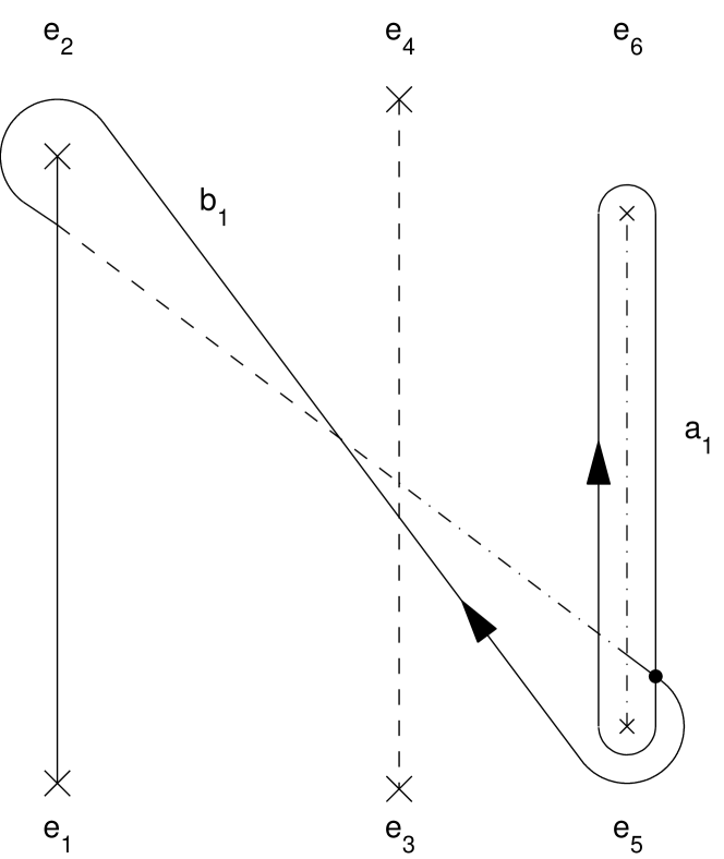
Figure 3. Basis of cycles of the elliptic curve $X$ of genus $1$. The solid line, dashed line and dashed-dotted lines denote paths on the first, second and third sheets correspondingly. The cuts between the first and second, second and the third and third and the first sheets are denoted as correspondingly

This curve is of genus 1 and admits the following behavior on the sheets at infinities

(6.3) $$\begin{split}z=\frac{1}{\xi},\quad&w=-\frac{2\,\mathrm{i}\,}{\xi^{2}}-\frac{\,\mathrm{i}\,}{2}\lambda_{2}\xi+O(\xi^{2})\quad\text{on the first sheet},\\ z=\frac{1}{\xi},\quad&w=\frac{2\,\mathrm{i}\,}{\xi^{2}}+\frac{\,\mathrm{i}\,}{4}(\lambda_{2}+\sqrt{\Delta})\xi+O(\xi^{2})\quad\text{on the second sheet},\\ z=\frac{1}{\xi},\quad&w=\frac{2\,\mathrm{i}\,}{\xi^{2}}+\frac{\,\mathrm{i}\,}{4}(\lambda_{2}-\sqrt{\Delta})\xi+O(\xi^{2})\quad\text{on the third sheet}.\end{split}$$

The holomorphic differential on $X$ be of the form

(6.4) $$du=\frac{(w-2\,\mathrm{i}\,z^{2})dz}{3w^{2}+4\,\mathrm{i}\,wz^{2}+4z^{4}+\lambda_{2}z+\lambda_{3}}.$$

Denote $A=\oint_{\mathfrak{a}}du$ its $\mathfrak{a}$-period, then the normalized holomorphic differential $dv=du/A$.

In the case considered we have $r_{2}=-r_{3}=r$,

(6.5) $$r=\frac{1}{A}\int\limits_{\infty_{1}}^{\infty_{2}}du.$$

Indeed, because of expansions (3.17) the function on the curve $w-2\,\mathrm{i}\,z^{2}$ has second order pole at the first sheet and first order zeros on the second and third sheets. Then the Abel theorem says $r_{2}+r_{3}=0$.

The auxiliary winding numbers (4.13) are computed with the aid of (3.17) as follows

(6.6) $$\begin{split}V^{(1)}&=\frac{1}{4A},\quad V^{(2)}=\frac{-\sqrt{\Delta}-\lambda_{2}}{8A\sqrt{\Delta}},\quad V^{(3)}=\frac{-\sqrt{\Delta}+\lambda_{2}}{8A\sqrt{\Delta}}.\\ W^{(1)}&=0,\quad W^{(2)}=\frac{\,\mathrm{i}\,\lambda_{3}\mu_{0}}{8A\sqrt{\Delta^{3}}},\quad W^{(2)}=-\frac{\,\mathrm{i}\,\lambda_{3}\mu_{0}}{8A\sqrt{\Delta^{3}}.}\end{split}$$

Therefore we have for the main winding numbers

(6.7) $$V=\frac{1}{2A},\quad W=0.$$

To perform further calculations it is convenient to transform the curve $X$ to the form of standard Weierstrass cubic. Namely there exists a birational transformation $T$

(6.8) $$\begin{split}T&:X\rightarrow\widetilde{X}\quad z=\frac{y-8\lambda_{2}}{8x},\quad w=\frac{\,\mathrm{i}\,}{32x^{2}}\left((y^{2}-8\lambda_{2})^{2}-8x^{3}\right)\\ T^{-1}&:\widetilde{X}\rightarrow{X}\quad x=4\,\mathrm{i}\,(w-2\,\mathrm{i}\,z^{2}),\quad y=32\,\mathrm{i}\,z(w-2\,\mathrm{i}\,z^{2})+8\lambda_{2}\end{split}$$

of the curve $X$ to $\widetilde{X}=(x,y)$

(6.9) $$y^{2}=4x^{3}-g_{2}x-g_{3}$$

with parameters

(6.10) $$g_{2}=64\lambda_{3},\quad g_{3}=-64\Delta.$$

The discriminant of $\widetilde{X}$, coincides with multiplier $27\Delta^{2}-64\lambda_{3}^{3}$ of the expression for the discriminant $X$. In what follows we shall use Weierstrass functions of the curve $\widetilde{X}$.

The transformation $T$ maps canonical holomorphic differential $du$ to $dx/y$. The point $2\omega r$ appeared to be a zero of the Weierstrass $\wp$-function,

(6.11) $$\wp(2\omega r)=0$$

what follows from the fact that the map $T$ is mapping $\infty_{1}$ of the curve $X$ to the $\infty$ of the curve $\widetilde{X}$ and $\infty_{2,3}$ of the curve $X$ to points $(0,\pm\,\mathrm{i}\,\sqrt{g_{3}})$ of curve $\widetilde{X}$. Remark that solution of (6.11) are given in [EZ82] in terms of Eisenstein series what will be of importance for developing computational algorithms.

Direct computations gives

(6.12) $$E_{1}=-E_{2}=E=-\frac{1}{2}(\zeta(2\omega r)-2\eta r),\quad N_{1,2}=0.$$

The equalities $W=0,N_{1,2}=0$ are in accordance to our analysis which leads to the statement that the time $t=t_{2}$ is stationary for the flow yielded the Manakov matrix $B$ (see 1.7).

The solution has the form

(6.13) $$\begin{split}q_{1,2}(x)&=2\,\mathrm{i}\,A_{1,2}\frac{\vartheta_{3}(Vx\pm r-D)}{\vartheta_{3}(Vx-D)}\mathrm{e}^{\pm Ex},\\ A_{1,2}&=\pm\frac{\,\mathrm{i}\,}{4\sqrt{2}A}\frac{\lambda_{2}\mp\sqrt{\Delta}}{\sqrt{\Delta}}\frac{\vartheta_{1}^{\prime}(0)}{\vartheta_{1}(r)}\mathrm{exp}\left\{\,\mathrm{i}\,\mathrm{arg}\left(\frac{\vartheta_{3}(D)}{\vartheta_{3}(\pm r-D)}\right)\right\},\end{split}$$

where $\theta(z)=\vartheta_{3}(z)$ is canonical $\theta$-function of the genus one curve (6.1), $D$ is arbitrary constant satisfying $\theta(D)\neq 0$. Substitution of the elliptic solution (6.13) to the expressions for levels of the integrals of motion (6.2) leads to equivalences and permit moreover to compute the link between periods $A$ and $2\omega$ as

(6.14) $$A=-2\omega.$$

It is remarkable that the simplest solution to the Manakov system, i.e. solution of genus one independent in time and as the result it soliton limit enable to yield Manakov soliton (1). We can guess (1) can be obtain as the result of degeneration of the genus three curve.

7. Summary: computational algorithm

This section is addressed to a reader who wants to know the computing algorithm without going through the arguments of the paper. The procedure to compute algebro-geometric solutions to the Vector Nonlinear Schrödinger equation

$$\,\mathrm{i}\,\frac{\partial q_{1}}{\partial t}+\frac{\partial^{2}q_{1}}{\partial x^{2}}+2\left(|q_{1}|^{2}+|q_{2}|^{2}\right)q_{1} = 0,$$

$$\,\mathrm{i}\,\frac{\partial q_{2}}{\partial t}+\frac{\partial^{2}q_{2}}{\partial x^{2}}+2\left(|q_{1}|^{2}+|q_{2}|^{2}\right)q_{2} = 0$$

can be formulate as follows.

• Fix positive integer $n\in\{2,3,\ldots\}$.

• Fix a polynomial in two variables (algebraic curve)

  $$f(z,w)=(w+\frac{\,\mathrm{i}\,}{2}(2z)^{n})(w-\frac{\,\mathrm{i}\,}{2}(2z)^{n})^{2}+(w-\frac{\,\mathrm{i}\,}{2}(2z)^{n})P_{n-1}(z)+\,\mathrm{i}\,P_{n-2}(z)=0,$$

  with arbitrary real polynomials $P_{n-2}$ and $P_{n-1}$ of degrees $n-2$ and $n-1$ correspondingly. Compute its genus $g$ by using [DvH01] and Maple. For polynomials $P_{n-2}$ and $P_{n-1}$ in general position $g=2n-3$.

• Compute the vector of holomorphic differentials $d\boldsymbol{u}(Q)=(du_{1}(Q),\ldots,du_{g}(Q))^{T}$.

  $$du_{j}(Q) =\frac{\,\mathrm{i}\,z^{j}}{\frac{\partial}{\partial w}f(z,w)}dz,\quad j=0,\ldots,n-3,$$

  $$du_{j}(Q) =\frac{z^{n-2-j}\left(w-\frac{\,\mathrm{i}\,}{2}(2z)^{n}\right)}{\frac{\partial}{\partial w}f(z,w)}\,dz,\quad j=n-2,\ldots,2n-3.$$

• Compute vector of normalized holomorphic differentials

  $$d\boldsymbol{v}(Q)=A^{-1}d\boldsymbol{u}(Q)$$

• Compute auxiliary winding vectors $\boldsymbol{V}^{(i)},\boldsymbol{W}^{(i)},\boldsymbol{Z}^{(i)}$, $i=1,2,3$ from expansions

  $$\left.\int\limits_{Q}^{P}d\boldsymbol{v}\right|_{P\to\infty_{i}}=O(1)+\boldsymbol{V}^{(i)}\xi+\boldsymbol{W}^{(i)}\xi^{2}+\boldsymbol{Z}^{(i)}\xi^{3}+\ldots,\quad i=1,2,3,$$

  Set for main winding vectors

  $$\boldsymbol{V} =\,\mathrm{i}\,\boldsymbol{V}^{(1)}-\,\mathrm{i}\,\boldsymbol{V}^{(2)}-\,\mathrm{i}\,\boldsymbol{V}^{(3)},\quad\boldsymbol{W}=4\,\mathrm{i}\,\boldsymbol{W}^{(1)}-4\,\mathrm{i}\,\boldsymbol{W}^{(2)}-4\,\mathrm{i}\,\boldsymbol{W}^{(3)}.$$

• Compute vectors $\boldsymbol{r}_{2,3}$

  $$\boldsymbol{r}_{2,3}=\int\limits_{\infty_{1}}^{\infty_{2,3}}d\boldsymbol{v}.$$

• Compute 6 constants

  $$E_{1,2} =\,\mathrm{i}\,\left(\partial_{\boldsymbol{V}^{(1)}}-\partial_{\boldsymbol{V}^{(2,3)}}\right)\mathrm{ln}\theta[\varepsilon](\boldsymbol{r}_{2,3})-\,\mathrm{i}\,\partial_{\boldsymbol{V}^{(3,2)}}\mathrm{ln}\left[{\theta[\varepsilon](\boldsymbol{r}_{3,2})}{\theta[\varepsilon](\boldsymbol{r}_{2,3}-\boldsymbol{r}_{3,2})}\right]$$

  $$-\,\mathrm{i}\,c_{1}^{(2,3)}-\,\mathrm{i}\,c_{1}^{(1)},$$

  $$N_{1,2} =4\,\mathrm{i}\,\left(\partial_{\boldsymbol{W}^{(1)}}-\partial_{\boldsymbol{W}^{(2,3)}}\right)\mathrm{ln}\theta[\varepsilon](\boldsymbol{r}_{2,3})-4\,\mathrm{i}\,\partial_{\boldsymbol{W}^{(3,2)}}\mathrm{ln}\left[{\theta[\varepsilon](\boldsymbol{r}_{3,2})}{\theta[\varepsilon](\boldsymbol{r}_{2,3}-\boldsymbol{r}_{3,2})}\right]$$

  $$-2\,\mathrm{i}\,\left(\partial^{2}_{\boldsymbol{V}^{(1)},\boldsymbol{V}^{(2,3)}}-\partial^{2}_{\boldsymbol{V}^{(2,3)},\boldsymbol{V}^{(1)}}\right)\mathrm{ln}\theta[\varepsilon](\boldsymbol{r}_{2,3})$$

  $$+2\,\mathrm{i}\,\partial^{2}_{\boldsymbol{V}^{(3,2)},\boldsymbol{V}^{(2,3)}}\mathrm{ln}\left[\frac{\theta[\varepsilon](\boldsymbol{r}_{3,2})}{\theta[\varepsilon](\boldsymbol{r}_{2,3}-\boldsymbol{r}_{3,2})}\right]-\,\mathrm{i}\,c_{2}^{(2,3)}-\,\mathrm{i}\,c_{2}^{(1)},$$

  $$\delta_{2,3} =\frac{\,\mathrm{i}\,}{\theta[\varepsilon](\boldsymbol{r}_{2,3})}\sqrt{\partial_{\boldsymbol{V}^{(2,3)}}\theta[\varepsilon](\boldsymbol{0})}\sqrt{\partial_{\boldsymbol{V}^{(1)}}\theta[\varepsilon](\boldsymbol{0})},$$

  where $[\varepsilon]$ be non-singular odd characteristic, $\partial_{\boldsymbol{V}}$, $\partial_{\boldsymbol{W}}$ and $\partial_{\boldsymbol{Z}}$ are directional derivatives,

  $$\partial_{\boldsymbol{V}}= \sum_{k=1}^{g}V_{k}\frac{\partial}{\partial v_{k}},\quad\partial^{2}_{\boldsymbol{V},\boldsymbol{W}}=\sum_{k=1}^{g}\sum_{l=1}^{g}V_{k}W_{l}\frac{\partial^{2}}{\partial v_{k}\partial v_{l}},\quad\text{etc.}$$

  and also 6 constants, at $i=1,2,3$,

  $$c_{1}^{(i)} =\frac{1}{2}\frac{\partial^{2}_{\boldsymbol{V}^{(i)},\boldsymbol{V}^{(i)}}\theta[\varepsilon](\boldsymbol{0})}{\partial_{\boldsymbol{V}^{(i)}}\theta[\varepsilon](\boldsymbol{0})}-\frac{\partial_{\boldsymbol{W}^{(i)}}\theta[\varepsilon](\boldsymbol{0})}{\partial_{\boldsymbol{V}^{(i)}}\theta[\varepsilon](\boldsymbol{0})},$$

  $$c_{2}^{(i)} =-\left(\frac{\partial_{\boldsymbol{W}^{(i)}}\theta[\varepsilon](\boldsymbol{0})}{\partial_{\boldsymbol{V}^{(i)}}\theta[\varepsilon](\boldsymbol{0})}\right)^{2}+\frac{1}{3}\frac{\partial^{3}_{\boldsymbol{V}^{(i)},\boldsymbol{V}^{(i)},\boldsymbol{V}^{(i)}}\theta[\varepsilon](\boldsymbol{0})}{\partial_{\boldsymbol{V}^{(i)}}\theta[\varepsilon](\boldsymbol{0})}+\frac{\partial_{\boldsymbol{Z}^{(i)}}\theta[\varepsilon](\boldsymbol{0})}{\partial_{\boldsymbol{V}^{(i)}}\theta[\varepsilon](\boldsymbol{0})}.$$

• The algebro-geometric solution is of the form

  $$q_{1,2}(x,t) =2\,\mathrm{i}\,A_{1,2}\frac{\theta\left(\boldsymbol{V}x+\boldsymbol{W}t-\boldsymbol{D}+\boldsymbol{r}_{2,3}\right)}{\theta\left(\boldsymbol{V}x+\boldsymbol{W}t-\boldsymbol{D}\right)}\mathrm{exp}\left\{-E_{1,2}x+N_{1,2}t\right\},$$

  $$A_{1,2} =\delta_{2,3}\mathrm{exp}\left\{\,\mathrm{i}\,\;\mathrm{arg}\left(\frac{\theta(\boldsymbol{D})}{\theta(\boldsymbol{r}_{2,3}-\boldsymbol{D})}\right)\right\},$$

  where $\boldsymbol{D}$ is arbitrary vector satisfying condition $\theta(\boldsymbol{D})\neq 0$.

8. Appendix

Write in addition to (6.6) the third auxiliary winding numbers

(8.1) $$Z^{(1)}=0,\quad Z^{(2,3)}=\pm\frac{\,\mathrm{i}\,}{16}\frac{\lambda_{2}\mu_{0}\lambda_{3}^{2}}{A\Delta^{\frac{5}{2}}}$$

The constants $c_{l}^{(k)},$ $l=1,2$ and $k=1,2,3$ are

(8.2) $$c_{1}^{(1)}==0,\quad c_{1}^{(2,3)}==\frac{\lambda_{3}(\lambda_{2}\pm\sqrt{\Delta})}{4\Delta}$$

and

$$c_{2}^{(1)} =-\frac{1}{48A^{2}}\frac{\vartheta_{1}^{\prime\prime\prime}(0)}{\vartheta_{1}^{\prime}(0)},$$

$$c_{2}^{(2,3)} =\frac{\,\mathrm{i}\,\mu_{0}\lambda_{3}^{2}(\,\mathrm{i}\,\mu_{0}-\lambda_{2}^{2}\pm\sqrt{\Delta})}{(\lambda_{2}\mp\sqrt{\Delta})^{2}\Delta^{2}}-\frac{1}{192A^{2}}\frac{(\lambda_{2}\pm\sqrt{\Delta})^{2}}{\Delta^{2}}\frac{\vartheta_{1}^{\prime\prime\prime}(0)}{\vartheta_{1}^{\prime}(0)}.$$

Compute first $E_{1}-E_{2}$. We have

$$E_{1}-E_{2} =\,\mathrm{i}\,(X_{12}-X_{13})-\,\mathrm{i}\,(X_{32}-X_{23})+\,\mathrm{i}\,(c_{1}^{(3)}-c_{1}^{(2)})$$

$$=2\,\mathrm{i}\,V^{(1)}\left(\mathrm{ln}\,\vartheta_{1}(r)\right)^{\prime}-\,\mathrm{i}\,(V^{(2)}+V^{(3)})\left(\mathrm{ln}\,\vartheta_{1}(2r)\right)^{\prime}-\frac{\,\mathrm{i}\,\lambda_{3}}{2\sqrt{\Delta}}$$

$$=\frac{\,\mathrm{i}\,}{4A}[4\omega\zeta(2\omega r)-8\eta\omega r]+\frac{\,\mathrm{i}\,}{4A}[2\omega\zeta(4\omega r)-8\eta\omega r]-\frac{\,\mathrm{i}\,\lambda_{3}}{2\sqrt{\Delta}}.$$

Apply the duplication formula

$$\zeta(2z)=2\zeta(z)+\frac{1}{2}\frac{\wp^{\prime\prime}(z)}{\wp^{\prime}(z)},$$

which in the case considered reads

$$\zeta(4\omega r)=\zeta(2\omega r)-\frac{2\lambda_{3}}{\sqrt{\Delta}}$$

to obtain

(8.3) $$E_{1}-E_{2}=V(4\omega\zeta(2\omega r)-8\eta\omega r)-\frac{\,\mathrm{i}\,\lambda_{3}}{\sqrt{\Delta}}\left(\frac{\omega}{A}+\frac{1}{2}\right).$$

Analogously obtain

$$E_{1}+E_{2} =2\,\mathrm{i}\,(X_{2ń}+X_{31})-\,\mathrm{i}\,(X_{32}+X_{23})-\,\mathrm{i}\,(c_{1}^{(3)}+c_{1}^{(2)})$$

$$=\,\mathrm{i}\,(V^{(3)}-V^{(2)})(2\left(\mathrm{ln}\,\vartheta_{1}(r)\right)^{\prime}-\left(\mathrm{ln}\,\vartheta_{1}(2r)\right)^{\prime})-\frac{\,\mathrm{i}\,\lambda_{2}\lambda_{3}}{2\Delta}$$

$$=-\frac{\,\mathrm{i}\,\lambda_{2}\lambda_{3}}{\Delta}\left(\frac{\omega}{A}+\frac{1}{2}\right).$$

To complete computation of $E_{1,2}$ we must find relation between period $A$ of the curve $X$ and period $2\omega$ of the curve $\widetilde{X}$. We shall do that by substituting (6.13) to the (6.2) which should lead to equivalence. We have

$$q_{1x}q_{2}-q_{2x}q_{1}=-4\delta_{2}\delta_{3}\mathrm{exp}[(E_{1}+E_{2})x]$$

$$\times\left\{\frac{V}{\vartheta_{1}(Vx^{\prime})^{2}}(\vartheta_{1}(Vx^{\prime}-r)\vartheta_{1}^{\prime}(Vx^{\prime}+r)-\vartheta_{1}(Vx^{\prime}+r)\vartheta_{1}^{\prime}(Vx^{\prime}-r))\right.$$

$$\left.\qquad\qquad+\frac{E_{2}-E_{1}}{\vartheta_{1}(Vx^{\prime})^{2}}\vartheta_{1}(Vx^{\prime}-r)\vartheta_{1}(Vx^{\prime}+r)\right\},$$

where $x^{\prime}=x-\frac{1}{2V}(1+\tau)$. Substituting instead of derivatives $\vartheta_{1}^{\prime}(z)$ Weierstrass $\zeta$-functions we transform the expression in the curly brackets to

$$\frac{\vartheta_{1}(Vx^{\prime}-r)\vartheta_{1}(Vx^{\prime}+r)}{\vartheta_{1}(Vx^{\prime})^{2}}\left[2\omega V\zeta(2Vx^{\prime}\omega+2\omega r)\right.$$

$$-\left.2\omega V\zeta(2Vx^{\prime}\omega-2\omega r)-8V\omega\eta r+E_{2}-E_{1}\right]$$

$$=\sigma(2\omega r)^{2}\mathrm{exp}\left\{-\frac{r^{2}\eta}{\omega}\right\}\wp(2\omega Vx^{\prime})$$

$$\times\left[4\omega V\zeta(2\omega r)-8V\eta\omega r+E_{2}-E_{1}+\frac{2\omega\sqrt{g_{3}}}{\wp(2\omega Vx^{\prime})}\right],$$

where we applied addition formula for the Weierstrass $\sigma$ and $\zeta$-functions and took into account (6.11). Because this quantity should be a constant with respect to $x$ we set

(8.4) $$E_{1}-E_{2}=4\omega V(\zeta(2\omega r)-2\eta r),\quad E_{1}+E_{2}=0$$

what in combination with (8.3) gives relation (6.14) between $\mathfrak{a}$-periods of the curve $X$ and $\widetilde{X}$. Therefore the derivation of expressions for $E_{1,2}$ given in (6.12) is completed. But let us continue the computation of the integral level. We have now

$$|q_{1x}q_{2}-q_{2x}q_{1}|^{2}=256\left|\omega^{4}\delta_{2}^{2}\delta_{3}^{2}g_{3}\frac{\vartheta_{1}(r)^{2}}{\vartheta_{1}(0)^{2}}\right|.$$

But

$$\delta_{2}^{3}\delta_{3}^{2}=\frac{\,\mathrm{i}\,\mu_{0}}{256A^{4}\Delta}\frac{\vartheta_{1}(0)^{2}}{\vartheta_{1}(r)^{2}}\quad\text{and}\quad g_{3}=-64\Delta,$$

what completes the derivation of equivalence.

It remains to show that $N_{1,2}=0$. Develop expression for $N_{1}$. It is the sum of 3 terms which are

$$-c_{2}^{(2)}-c_{2}^{(1)}=-\frac{\eta\omega(-3\lambda_{2}^{2}+10\,\mathrm{i}\,\mu_{0}+\lambda_{2}\sqrt{\Delta})}{8A^{2}\Delta}-\frac{\,\mathrm{i}\,\mu_{0}\lambda_{3}^{2}(\,\mathrm{i}\,\mu_{0}-\lambda_{2}^{2}+\lambda_{2}\sqrt{\Delta})}{\Delta^{2}(\lambda_{2}-\sqrt{\Delta})^{2}}$$

$$2(W^{(1)}-W^{(2)}+W^{(3)})(\mathrm{ln}\,\vartheta_{1}(r))^{\prime}-2W^{(3)}(\mathrm{ln}\,\vartheta_{1}(2r))^{\prime}=\frac{\,\mathrm{i}\,\lambda_{3}^{2}\mu_{0}\omega}{A\Delta^{2}}$$

$$2((V^{(1)})^{2}+(V^{(2)})^{2}+(V^{(3)})^{2})(\mathrm{ln}\,\vartheta_{1}(r))^{\prime\prime}-2(V^{(3)})^{2}(\mathrm{ln}\,\vartheta_{1}(2r))^{\prime\prime}$$

$$=\frac{\eta\omega(-3\lambda_{2}^{2}+10\,\mathrm{i}\,\mu_{0}+\lambda_{2}\sqrt{\Delta})}{8A^{2}\Delta}-\frac{\omega^{2}\lambda_{3}^{2}(\lambda_{2}+\sqrt{\Delta})^{2}}{4A^{2}\Delta^{2}}.$$

Taking into the account equality (6.11) and substituting then (6.14) to the sum we obtain necessary equality. The equality $N_{2}=0$ is derived in analogous way.

It could be also of interest to check by direct substitution that solution (6.13) satisfies to the Manakov system. To check that we first compute

(8.5) $$2(|q_{1}(x,t)|^{2}+|q_{2}(x,t)|^{2})=8(\delta_{2}^{2}+\delta_{3}^{2})\frac{\vartheta_{3}(Vx^{\prime}+r)\vartheta_{3}(Vx^{\prime}-r)}{\vartheta_{3}(Vx)^{2}}$$

$$=-\frac{\vartheta_{1}^{\prime}(0)}{8\omega^{2}}\frac{\vartheta_{3}(Vx^{\prime}+r)\vartheta_{3}(Vx^{\prime}-r)}{\vartheta_{3}(Vx)^{2}\vartheta_{1}(r)^{2}}-\frac{\sigma(2\omega Vx+2\omega r)\sigma(2\omega Vx-2\omega r)}{2\sigma^{2}(2*\omega V)\sigma^{2}(2\omega r)}$$

$$=-\frac{1}{2}\wp(2\omega Vx),$$

where we used again in the Weierstrass addition theorem (6.11). Further the first derivative

$$\frac{\partial}{\partial x} q_{1}(x,t)$$

$$=q_{1}(x,t)\left(2V\omega\zeta(2\omega r)-4V\eta\omega-E+\frac{V\omega(\wp^{\prime}(2\omega V)-\,\mathrm{i}\,\sqrt{g_{3}})}{\wp(2\omega Vx)}\right)$$

The first 3 terms in brackets vanish because of expression for $E$ given in (6.12). Therefore

(8.6) $$\frac{\partial^{2}}{\partial x^{2}}q_{1}(x,t)$$

$$=q_{1}(x,t)\left[\left(\frac{V\omega(\wp^{\prime}(2\omega V)-\,\mathrm{i}\,\sqrt{g_{3}})}{\wp(2\omega Vx)}\right)^{2}+\frac{\partial}{\partial x}\left(\frac{V\omega(\wp^{\prime}(2\omega V)-\,\mathrm{i}\,\sqrt{g_{3}})}{\wp(2\omega Vx)}\right)\right]$$

$$=\frac{1}{2}q_{1}(x,t)\wp(2\omega Vx).$$

Combining (8.5) and (8.6) we obtain the equiality (1.1). Validity of the (1.2) is proved analogously.

References

- [AHH90] M. R. Adams, J. Harnad, and J. Hurtubise, Isospectral Hamiltonian flows in finite and infinite dimension. II. Integration of flows, Commun. Math. Phys. 134 (1990), 555–585.
- [Bak95] H. F. Baker, Abel’s theorem and the allied theory of theta functions, Cambridge Univ. Press, Cambridge, 1897, reprinted 1995.
- [BBE+94] E. D. Belokolos, A. I. Bobenko, V. Z. Enolskii, A. R. Its, and V. B. Matveev, Algebro Geometric Approach to Nonlinear Integrable Equations, Springer, Berlin, 1994.
- [BEL97] V. M. Buchstaber, V. Z. Enolskii, and D. V. Leykin, Kleinian functions, hyperelliptic Jacobians and applications, Reviews in Mathematics and Mathematical Physics (London) (S. P. Novikov and I. M. Krichever, eds.), vol. 10:2, Gordon and Breach, 1997, pp. 1–125.
- [CEEK00] P. L. Christiansen, J. C. Eilbeck, V. Z. Enolskii, and N. A. Kostov, Quasi periodic solutions of Manakov type coupled nonlinear Schrödinger equations, Proc. R. Soc. Lond. A 456 (2000), 2263–2281.
- [DvH01] B. Deconinck and M. van Hoeij, Computing Riemann matrices of algebraic curves, Physica D 152-153 (2001), 28–46.
- [EZ82] M Eichler and D Zagier, On the zeroes of the Weierstrass -function, Math. Ann. 258 (1982), 399–407.
- [EGH00] V. Z. Enolskii, F. Gesztesy, and H. Holden, The classical massive Thirring system revisited, Stochastic Processes, Physics and Geometry: New Interplays. I. A Volume in Honor of S. Albeverio, Canadian Mathematical Society Conference Proceeding Series (Providence, RI, USA) (F. Gesztesy, H. Holden, J. Jost, S. Paycha, M. Röckner, and S. Scarlatti, eds.), American Mathematical Society for Canadian Mathematical Society, 2000.
- [FK80] H. Farkas, I. Kra Riemann surfaces, Springer, 1980.
- [Fay73] J. D. Fay, Theta functions on Riemann surfaces, Lectures Notes in Mathematics (Berlin), vol. 352, Springer, 1973.
- [FMMW00] M. G. Forest, D. W. McLaughlin, D. J. Muraki, and O. C. Wright, Nonfocusing Instabilities in Coupled, Integrable Nonlinear Schrödinger pdes, J. Nonlinear Sci. 10 (2000), 291–331.
- [FSW00] M. G. Forest, S. P. Sheu, and O. C. Wright, On the construction of orbits homoclinic to plane waves in integrable coupled nonlinear Schrödinger system, Phys. Lett. A 266 (2000), no. 1, 24–33.
- [GH03] F. Gesztesy and H. Holden, Soliton Equations and Their Algebro-Geometric Solutions. -Dimensional Continuous Models, Cambridge University Press, Cambridge, U.K., 2003.
- [Its76] A. R. Its, Inversion of hyperelliptic integrals and integration of nonlinear differential equations, Vestnik Leningrad University, N 7 (Ser. Math. Mekh. Astr. vyp. 2) 7 (1976), 39-46; English transl. in Vestnik Leningrad University, Math. 9 (1981), 121 - 129.
- [IK76] A. R. Its, V. P. Kotlyarov, Explicit formulas for solutions of the nonlinear Schrödinger equation, Dokl. Akad. Nauk Ukraine. SSSR, ser. A 11 (1976), 965 - 968.
- [Jor92] J. Jorgenson, On directional derivatives of the theta function along its divisor, Israel J.Math. 77 (1992), 274–284.
- [Kri77] I. M. Krichever, The method of algebraic geometry in the theory of nonlinear equations, Russian. Math. Surveys 32 (1977), 180–208.
- [Man74] S. V. Manakov, On the theory of two-dimensional stationary self-focusing of electromagnetic waves, Soviet JETP 38 (1974), 248–253.
- [Pre85] E. Previato, Hyperelliptic quasiperiodic and soliton solutions of the nonlinear Schrödinger equation, Duke Math. J. 52 (1985), no. 2, 328–377.
- [WF00] O. C. Wright and M. G. Forest, On the Bäcklund-gauge transformation and homoclinic orbits of a coupled nonlinear Schrödinger system, Physica D: Nonlinear Phenomena 141 (2000), no. 1-2, 104–116.
- [Wri99] O. C. Wright, The stationary equations of a coupled nonlinear Schrödinger system, Physica D 126 (1999), no. 3-4, 275–289.