On the Quantum variance of matrix elements for the cat map on the 4-dimensional torus

Abstract.

For many classically chaotic systems, it is believed that in the semiclassical limit, the matrix elements of smooth observables approach the phase space average of the observable. In the approach to the limit the matrix elements can fluctuate around this average. Here we study the variance of these fluctuations, for the quantum cat map on $\mathbb{T}^{4}$. We show that for certain maps and observables, the variance has a different rate of decay, than is expected for generic chaotic systems.

1. Introduction

The basic question of “Quantum Chaos” is what signatures of the classical (chaotic) dynamics one can still find in the quantized system. One important such signature is given by the asymptotic behavior of expectation values, and the limit distribution around their average in the semiclassical limit.

For classically chaotic systems, the average of smooth observables on phase space, along the trajectories of the system, tend almost always to the phase space average (i.e., the classical dynamics is ergodic). The quantum analog of this, following the correspondence principle, is that the expectation values of an observable should tend to the phase space average of the observable in the semiclassical limit. The first result in this direction is “Šhnirel’man’s theorem”, which states that at least in the sense of convergence in the mean square, when taking Planck’s constant $h\rightarrow 0$, the matrix elements converge to the phase space average  [2, 3, 19, 20]. This notion is usually referred to as “Quantum Ergodicity” (Q.E.).

In the approach to the limit, the different matrix elements can fluctuate about their classical limit. In  [7] Feingold and Peres proposed a formula for the variance of the fluctuations in the semiclassical limit. As mentioned above, according to Šhnirel’man’s theorem the variance vanishes as $h\rightarrow 0$. Nevertheless, after normalizing by an appropriate power of $h$, the Feingold-Peres formula relates the variance of the matrix elements to classical correlations of the observable. In  [5], Eckhardt et al. developed a semiclassical theory for the variance of these fluctuations, giving support for the validity of the Feingold-Peres formula, and suggesting that after normalizing by the variance, the fluctuation should be Gaussian (at least for hyperbolic systems). The analysis in [5], for the fluctuations of the matrix elements, can be extended to deal with quantum maps  [18]. In particular, for generic hyperbolic quantum maps on the 2d-torus $\mathbb{T}^{2d}$, it predicts Gaussian distribution with variance of order $\frac{\alpha}{N^{d}}$, where $N=1/h$ plays the role of the inverse of Planck’s constant, and $\alpha$ is related to the classical variance of the observable.

A fundamental example for a quantum map on the torus is the quantum cat map, originally introduced by Hannay and Berry [9]. Here the classical dynamics is simply the iteration of a symplectic linear map $A\in\mathrm{Sp}(2d,\mathbb{Z})$ on $\mathbb{T}^{2d}=\mathbb{R}^{2d}/\mathbb{Z}^{2d}$. When $A$ has no roots of unity for eigenvalues, the classical dynamics is ‘chaotic’ (i.e., ergodic and mixing).

For the quantization of the cat map, the admissible values of Planck’s constant are inverses of integers, and the space of quantum states is then $\mathcal{H}_{N}=L^{2}[(\mathbb{Z}/N\mathbb{Z})^{d}]$. The semiclassical limit is achieved by taking $N\rightarrow\infty$, and we restrict the discussion to the case where $N$ is prime. For $f\in C^{\infty}(\mathbb{T}^{2d})$ a smooth observable, we denote by $\mbox{Op}_{N}(f):\mathcal{H}_{N}\rightarrow\mathcal{H}_{N}$ its quantization. The quantization of the map $A$, is then a unitary operator $U_{N}(A)$ acting on $\mathcal{H}_{N}$.

For $d=1$, this model was studied extensively and it exhibits some interesting features [9, 6, 16, 15]. It is shown to be (Q.E.), but not (Q.U.E.). However, in [15] Kurlberg and Rudnick introduced a group of symmetries of the system, a family of commuting unitary maps of $\mathcal{H}_{N}$ that commute with $U_{N}(A)$. These operators are called Hecke operators, in analogy to a similar setup on the modular surface [10]. The space $\mathcal{H}_{N}$ has an orthonormal basis consisting of joint eigenstates $\{\phi_{j}\}_{j=1}^{N}$ called “Hecke eigenstates”. For these states the system is shown to be (Q.U.E.) [15].

In [16] Kurlberg and Rudnick studied the fluctuation of the matrix elements for the desymmetrized system and gave a conjecture for the limit distribution, which is radically different from the behavior expected in the generic case. In particular, a fourth moment calculation for the distribution showed that it is not Gaussian. Furthermore, though the variance of the fluctuation is of order $\frac{1}{N}$ as expected, the classical factor is different from the classical variance, in contrast to the Feingold-Peres formula (for comparison see [16]).

Remark 1.1.

In [17] Luo and Sarnak showed similar behavior of the variance for Hecke eigenforms on the modular surface. For this system, the variance of the fluctuations after appropriately normalizing, does not converge to the classical variance of the observable. However the classical variance can be recovered, after inserting some arithmetic correction. Furthermore the limit distribution for the Hecke eigenforms is again not Gaussian (pending on conjectures of Keating and Snaith [11]).

In this note we look at the matrix elements for quantized cat maps on $\mathbb{T}^{4}$, and the variance of their fluctuations. Here we find that for certain maps and observables, the variance has a different rate of decay than that predicted by the Feingold-Peres formula.

Let $A\in\mathrm{Sp}(4,\mathbb{Z})$ be a matrix with $4$ distinct eigenvalues. For the dynamics to be ergodic we assume that $A$ has no roots of unity for eigenvalues. We further assume that the vector space $\mathbb{Q}^{4}$ decomposes into two rational orthogonal symplectic subspaces, invariant under the action of $A$. Denote by $Z_{1},Z_{2}$, the lattices obtained by intersecting these subspaces with $\mathbb{Z}^{4}$.

Analogously to the treatment of the case $d=1$ we introduce Hecke operators, a family of commuting operators that commute with $U_{N}(A)$, and consider a basis of joint eigenstates $\left\{\phi_{j}\right\}_{j=1}^{N^{2}}$, referred to as the Hecke basis. For any smooth observable $f\in C^{\infty}(\mathbb{T}^{4})$, denote the quantum variance in the Hecke basis by

$$S_{2}(f,N)=\frac{1}{N^{2}}\sum_{j=1}^{N^{2}}\bigg{|}\langle\mbox{Op}_{N}(f)\phi_{j},\phi_{j}\rangle-\int_{\mathbb{T}^{4}}f\bigg{|}^{2}.$$

Theorem 1.

Let $f(\vec{x})=e^{2\pi i\vec{n}\cdot\vec{x}},\;\vec{n}\neq 0$. Then, as $N\rightarrow\infty$ through primes, the variance of these observables is given by

$$S_{2}(f,N)=\left\{\begin{array}[]{cc}\frac{1}{N}+O(\frac{1}{N^{2}})&\mbox{if }\vec{n}\in Z_{1}\cup Z_{2},\\ \frac{1}{N^{2}}+O(\frac{1}{N^{3}})&\mbox{ otherwise }.\end{array}\right.$$

This result is in contrast to the expected rate of $\frac{1}{N^{2}}$, predicted to hold for all observables in generic hyperbolic systems.

Remark 1.2.

This result can be extended to any smooth observable $f\in C^{\infty}(\mathbb{T}^{4})$, to state that $S_{2}(f,N)=\frac{V_{1}(f)}{N^{2}}+O(\frac{1}{N^{3}})$, if the Fourier coefficients of $f$ are supported outside the lattices $Z_{1}\cup Z_{2}$, and $S_{2}(f,N)=\frac{V_{2}(f)}{N}+O(\frac{1}{N^{2}})$ otherwise. The terms $V_{1}(f),V_{2}(f)$ can be expressed as quadratic forms in the Fourier coefficients of $f$, see [12] for more details.

After knowing the variance of the fluctuation, we can renormalize the matrix elements and consider the limit distribution. We present some numerical calculations of this distribution, for the two types of elementary observables (figures 1,2 respectively). The numerical evidence suggests that when $\vec{n}\in Z_{1}\cup Z_{2}$, the distribution of the normalized matrix elements is given by the semicircle law, where otherwise after appropriately normalizing, it corresponds to the product of two semicircle random variables. This result, is in agreement with the conjecture presented in [16] for the limit distribution for the cat map on $\mathbb{T}^{2}$.

Furthermore, assuming that all matrix elements are roughly of the same order, the square root of the variance obtained here, gives an estimate of the rate of their decay. In figure 3, we present numerical calculation for this decay, strongly supporting the validity of this estimate.

2. Background

The full details for the cat map and it’s quantization can be found in  [15] for one dimensional system, and in [1, 12] for higher dimensions. We briefly review the setup for the quantization of the cat map on $\mathbb{T}^{4}$.

2.1. Classical dynamics

The classical dynamics are given by the iteration of a symplectic linear map $A\in\mathrm{Sp}(4,\mathbb{Z})$.

$$\vec{x}=\left(\begin{array}[]{c}\vec{p}\\ \vec{q}\\ \end{array}\right)\in\mathbb{T}^{4}\mapsto A\vec{x}.$$

Given an observable $f\in C^{\infty}(\mathbb{T}^{4})$, the classical evolution defined by $A$ is $f\mapsto f\circ A$. If $A$ has no eigenvalues that are roots of unity then the classical dynamics is ergodic and mixing [14].

2.2. Quantum kinematics

For doing quantum mechanics on the torus, one takes Planck’s constant to be $1/N$, as the Hilbert space of states one takes $\mathcal{H}_{N}=L^{2}((\mathbb{Z}/N\mathbb{Z})^{2})$, where the inner product is given by:

$$\langle\phi,\psi\rangle=\frac{1}{N^{2}}\sum_{\vec{y}\mod{N}}\phi(\vec{y})\overline{\psi(\vec{y})}.$$

For $\vec{n}=(\vec{n}_{1},\vec{n}_{2})\in\mathbb{Z}^{4}$ (where $\vec{n}_{i}\in\mathbb{Z}^{2}$), define elementary operators $T_{N}(\vec{n})$ acting on $\psi\in\mathcal{H}_{N}$ via:

(2.1) $$T_{N}(\vec{n})\psi(\vec{y})=e_{N}(\frac{\vec{n}_{1}\cdot\vec{n}_{2}}{2})e_{N}(\vec{n}_{2}\cdot\vec{y})\psi(\vec{y}+\vec{n}_{1}^{t}),$$

where $e_{N}(x)=e^{\frac{2\pi ix}{N}}$

For any smooth classical observable $f\in C^{\infty}(\mathbb{T}^{4})$ with Fourier expansion $f(\vec{x})=\sum_{\vec{n}\in\mathbb{Z}^{4}}\hat{f}(\vec{n})e^{2\pi i\vec{n}\cdot\vec{x}}$, its quantization is given by

$$Op_{N}(f)=\sum_{\vec{n}\in\mathbb{Z}^{4}}\hat{f}(\vec{n})T_{N}(\vec{n}).$$

The main properties of the elementary operators $T_{N}(\vec{n})$ are summarized in the following proposition.

Proposition 2.1.

For the operators $T_{N}(\vec{n})$ defined above:

1. $T_{N}(\vec{n})$ only depends on $\vec{n}\mod{2N}$.

2. $T_{N}(\vec{n})$ are unitary operators.

3. The composition of two elementary operators is

   $$T_{N}(\vec{m})T_{N}(\vec{n})=e_{2N}(\omega(\vec{m},\vec{n}))T_{N}(\vec{n}+\vec{m}),$$

   where $\omega(\vec{m},\vec{n})=\vec{m}_{1}\cdot\vec{n}_{2}-\vec{m}_{2}\cdot\vec{n}_{1}$, is the symplectic inner product.

4. If $\vec{n}=0\pmod{N}$, then $T_{N}(\vec{n})=(-1)^{(\vec{n}_{1}\cdot{\vec{n}_{2}})}I$.

These properties are easily derived from equation 2.1. Moreover, these properties uniquely characterize these operators, in the sense that if $\widetilde{T}_{N}(\vec{n})$ are operators acting on an $N^{2}$-dimensional Hilbert space fulfilling the above properties, then they are unitarily equivalent to $T_{N}(\vec{n})$.

2.3. Quantum dynamics:

For $A\in\mathrm{Sp}(4,\mathbb{Z})$ which satisfies certain parity conditions (namely $A=I\!\pmod{2}$), we assign unitary operators $U_{N}(A)$, acting on $L^{2}((\mathbb{Z}/N\mathbb{Z})^{2})$ having the following important properties:

1. “Exact Egorov”: For all observables $f\in C^{\infty}(\mathrm{\mathbb{T}}^{4})$

   $$U_{N}(A)^{-1}Op_{N}(f)U_{N}(A)=Op_{N}(f\circ A).$$

2. The quantization depends on $A$ modulo $2N$.

3. The quantization preserves commutation relations:
   if $AB=BA\!\pmod{2N}$ then $U_{N}(A)U_{N}(B)=U_{N}(B)U_{N}(A)$.

Note that if we multiply the operators by arbitrary phases, then all the above properties still hold. In fact the converse also holds, that is if $\tilde{U}_{N}(A)$ is an operator satisfying these properties, then $\tilde{U}_{N}(A)=e^{i\alpha}U_{N}(A)$.

Remark 2.1.

Eventually, we are interested in the eigenfunctions of these operators, which are not affected by the choice of phase. Thus, in order to simplify the discussion we do not set explicit phases for the quantization. However, we note that one can make a specific choice of phases for which this quantization is multiplicative, $U_{N}(AB)=U_{N}(A)U_{N}(B)$. In particular this implies property (3) above, indeed holds for any choice of phases.

Since we assume that $N$ is odd, and the quantization factors through the group

$$\left\{B\in\mathrm{Sp}(4,\mathbb{Z}/2N\mathbb{Z})|B=I\!\!\!\!\!\pmod{2}\right\}\simeq\mathrm{Sp}(4,\mathbb{Z}/N\mathbb{Z}),$$

we can define a (projective) representation of $\mathrm{Sp}(4,\mathbb{Z}/N\mathbb{Z})$:
For any element $B\in\mathrm{Sp}(4,\mathbb{Z}/N\mathbb{Z})$, let $\bar{B}\in\mathrm{Sp}(4,\mathbb{Z}/2N\mathbb{Z})$ be the unique element s.t. $B=\bar{B}\pmod{N},\;\;\bar{B}=I\pmod{2}$, and identify $U_{N}(B):=U_{N}(\bar{B})$. For the rest of this note we will use this convention for the quantization of $\mathrm{Sp}(4,\mathbb{Z}/N\mathbb{Z})$.

2.4. Hecke eigenfunctions

Let $A\in\mathrm{Sp}(4,\mathbb{Z})$, $A=I\!\!\pmod{2}$ and let $C(N,A)$ be a maximal commutative subgroup of $\mathrm{Sp}(4,\mathbb{Z}/N\mathbb{Z})$, which includes $A$ modulo $N$.

Remark 2.2.

In general, this group is not necessarily unique. However if all the eigenvalues of $A\!\!\!\mod{N}$ are distinct then $C(N,A)$ is unique. For an explicit construction see [12].

Since the quantization preserves commutation relations, the operators $U_{N}(B)$, $B\in C(N,A)$ form a family of commuting operators, called Hecke operators. Functions $\phi\in\mathcal{H}_{N}$ that are simultaneous eigenfunctions of all the Hecke operators are called Hecke eigenfunctions, and a basis consisting of Hecke eigenfunctions is called a Hecke basis. By definition $A\in C(N,A)$, consequently any Hecke eigenfunction is in particular also an eigenfunction of $U_{N}(A)$.

3. Reduction to lower dimension

Let $A\in\mathrm{Sp}(4,\mathbb{Z}),\;A=I\pmod{2}$, with 4 distinct eigenvalues. Further assume that the vector space $\mathbb{Q}^{4}$, decomposes into two (rational) symplectic subspaces, invariant under the action of $A$. In this case, the Hecke group $C(N,A)=\bar{C}_{1}(N,A)\times\bar{C}_{2}(N,A)$ is a direct product, each term $\bar{C}_{i}(N,A)$, can be identified with a lower dimensional Hecke group of a corresponding matrix in $\mbox{SL}(2,\mathbb{Z}/N\mathbb{Z})$. Correspondingly, the Hecke operators and eigenfunctions are a tensor product of the appropriate lower dimensional Hecke operators and eigenfunctions.

3.1. Reduction of Hecke group

For each invariant subspace, take a symplectic basis $e_{i},f_{i}\in\mathbb{Q}^{4}$, that is $\omega(e_{i},e_{j})=\omega(f_{i},f_{j})=0$ and $\omega(e_{i},f_{j})=\delta_{i,j}$. For a sufficiently large prime $N$, take $\bar{e_{i}},\;\bar{f_{i}}\in(\mathbb{Z}/N\mathbb{Z})^{4}$, through reduction of $e_{i}$ and $f_{i}$ modulo $N$ respectively. This induces a decomposition of $(\mathbb{Z}/N\mathbb{Z})^{4}=E_{1}\oplus E_{2}$ into two orthogonal symplectic subspaces invariant under the action of $A\!\!\mod{N}$.

For $\vec{n}\in\mathbb{Z}^{4}$, denote by $(\bar{n}_{1},\bar{n}_{2})\in(\mathbb{Z}/N\mathbb{Z})^{2}\times(\mathbb{Z}/N\mathbb{Z})^{2}$ the restriction of $\vec{n}\mod{N}$, to $E_{1}\oplus E_{2}$ in the symplectic basis. Since this is a symplectic decomposition then for any $\vec{n},\vec{m}\in\mathbb{Z}^{4}$

(3.1) $$\omega(\vec{n},\vec{m})=\omega(\bar{n}_{1},\bar{m}_{1})+\omega(\bar{n}_{2},\bar{n}_{2})\pmod{N}.$$

This decomposition induces a map

$$i_{N}:\mbox{SL}(2,\mathbb{Z}/N\mathbb{Z})\times\mbox{SL}(2,\mathbb{Z}/N\mathbb{Z})\hookrightarrow\mathrm{Sp}(4,\mathbb{Z}/N\mathbb{Z}).$$

If we denote by $A_{i}\in\mbox{SL}(2,\mathbb{Z}/N\mathbb{Z})$ the restriction of $A\pmod{N}$ to $E_{i}$ in the symplectic basis, then $i_{N}(A_{1},A_{2})\equiv A\pmod{N}$.

Lemma 3.1.

Let $\bar{C}_{i}(N,A)\subseteq\mbox{SL}(2,\mathbb{Z}/N\mathbb{Z})$ be maximal commutative subgroups which include $A_{i}$, $i=1,2$ respectively. Then the map $i_{N}$ defined above, maps the group $\bar{C}_{1}(N,A)\times\bar{C}_{2}(N,A)$ isomorphically onto $C(N,A)$.

Proof.

The map $i_{N}:\bar{C}_{1}(N,A)\times\bar{C}_{2}(N,A)\hookrightarrow C(N,A)$, is clearly injective. Thus, it is sufficient to show that this map is onto. Let $B\in\mathrm{Sp}(4,\mathbb{Z}/N\mathbb{Z})$, be a matrix that commutes with $A\pmod{N}$. We can assume $N$ is large enough so that $A\pmod{N}$ has 4 distinct eigenvalues in $F_{\!\!N^{2}}$. Consequently, the spaces $E_{i}$ are also invariant under the action of $B$. Thus if we denote by $B_{i}\in\mbox{SL}(2,\mathbb{Z}/N\mathbb{Z})$ the restriction of $B$ to $E_{i}$, in the symplectic basis, then $i_{N}(B_{1},B_{2})=B$. ∎

3.2. Quantization of Hecke group

Let $T_{N}^{(1)}(\cdot),U_{N}^{(1)}(\cdot)$ be the quantized elementary observables and propagators for $\mathbb{T}^{2}$. For $\vec{n}\in\mathbb{Z}^{4}$, identify $\bar{n}_{1},\bar{n}_{2}$ defined above with elements of $(\mathbb{Z}/2N\mathbb{Z})^{2}$ by requiring

(3.2) $$\bar{n}_{1}=(n_{1},n_{3}),\;\bar{n}_{2}=(n_{2},n_{4})\pmod{2}.$$

We can also identify $B_{i}\in\bar{C}_{i}(N,A)$, as elements of $\mbox{SL}(2,\mathbb{Z}/2N\mathbb{Z})$ by requiring them to be congruent to $I$ modulo $2$.

Proposition 3.2.

There is a unitary mapping

$$\mathcal{U}:L^{2}(\mathbb{Z}/N\mathbb{Z})^{2}\rightarrow L^{2}(\mathbb{Z}/N\mathbb{Z})\otimes L^{2}(\mathbb{Z}/N\mathbb{Z}),$$

such that:

1. For any $\vec{n}\in\mathbb{Z}^{4}$,

   $$\mathcal{U}T_{N}(\vec{n})\mathcal{U}^{-1}=T^{(1)}_{N}(\bar{n}_{1})\otimes T^{(1)}_{N}(\bar{n}_{2}).$$

2. For any $B\in C(N,A)$,

   $$\mathcal{U}U_{N}(B)\mathcal{U}^{-1}=U^{(1)}_{N}(B_{1})\otimes U^{(1)}_{N}(B_{2}).$$

Proof.

It is easily verified from 3.1, 3.2 that $\widetilde{T}_{N}(\vec{n})=T^{(1)}_{N}(\bar{n}_{1})\otimes T^{(1)}_{N}(\bar{n}_{2})$ obey the same relation as in proposition 2.1. Thus, from uniqueness they are unitarily equivalent.

As for the second part, recall $U^{(1)}_{N}(B_{1})$ and $U^{(1)}_{N}(B_{2})$ both satisfy the Egorov identity, and we showed that $\mathcal{U}T_{N}(\vec{n})\mathcal{U}^{-1}=T^{(1)}_{N}(\bar{n}_{1})\otimes T^{(1)}_{N}(\bar{n}_{2})$. Consequently, if we define $\tilde{U}_{N}(B)=\mathcal{U}^{-1}U^{(1)}_{N}(B_{1})\otimes U^{(1)}_{N}(B_{2})\mathcal{U}$, then $\tilde{U}_{N}(B)$ satisfies the Egorov identity as well:

$$\tilde{U}_{N}(B)^{-1}T_{N}(\vec{n})\tilde{U}_{N}(B)=T_{N}(\vec{n}B).$$

Thus, from the uniqueness of the quantization

$$\mathcal{U}U_{N}(B)\mathcal{U}^{-1}=U^{(1)}_{N}(B_{1})\otimes U^{(1)}_{N}(B_{2}).$$

∎

Remark 3.1.

In fact, one can use this procedure to define the phases for the quantization of the Hecke group. Consequently, if the phases for the quantized two dimensional maps are chosen so that the quantization is multiplicative (as done in [15]), then the quantization of the Hecke group would be multiplicative as well.

3.3. Hecke eigenfunctions

Let $\left\{\phi^{1}_{j}\right\}_{j=1}^{N},\left\{\phi^{2}_{j}\right\}_{j=1}^{N}\in L^{2}(\mathbb{Z}/N\mathbb{Z})$, be joint eigenfunctions of all the Hecke operators $U_{N}^{(1)}(B_{i}),\;B_{i}\in C_{i}(N,A)$ $i=1,2$ respectively. Correspondingly, $\phi_{j_{1},j_{2}}=\mathcal{U}^{-1}(\phi_{j_{1}}^{1}\otimes\phi_{j_{2}}^{2})$, are eigenfunctions of all the operators $\left\{U_{N}(B)|B\in C(N,A)\right\}$, and hence $\left\{\phi_{j_{1},j_{2}}\right\}_{j_{1},j_{2}=1}^{N}$ is a Hecke basis of $L^{2}(\mathbb{Z}/N\mathbb{Z})^{2}$. In this basis, the matrix elements of the elementary observables $T_{N}(\vec{n})$, are given by

(3.3) $$\langle T_{N}(\vec{n})\phi_{j_{1},j_{2}},\phi_{j_{1},j_{2}}\rangle=\langle T^{(1)}_{N}(\bar{n}_{1})\phi^{1}_{j_{1}},\phi^{1}_{j_{1}}\rangle\langle T^{(1)}_{N}(\bar{n}_{2})\phi^{2}_{j_{2}},\phi^{2}_{j_{2}}\rangle.$$

Remark 3.2.

The joint eigenspaces of all the operators $U_{N}^{(1)}(B_{i}),\>B_{i}\in C_{i}(N,A)$, are one dimensional (except for the eigenspace corresponding to the trivial character) [12]. Correspondingly, any Hecke eigenfunction is of the form defined above, except for Hecke eigenfunctions corresponding to the trivial character, which are of the form $\phi=\mathcal{U}^{-1}(a\phi_{1}^{1}\otimes\phi_{1}^{2}+b\phi_{2}^{1}\otimes\phi_{2}^{2})$, where $\phi_{1}^{i},\phi_{2}^{i}\in L^{2}(\mathbb{Z}/N\mathbb{Z})$ correspond to the trivial character, and $|a|^{2}+|b|^{2}=1$.

4. Variance of matrix elements

We now turn to prove theorem 1. We will concentrate on the elementary observables $f(\vec{x})=e^{2\pi\vec{n}\cdot\vec{x}}$ with corresponding quantum operators $\mbox{Op}_{N}(f)=T_{N}(\vec{n})$, and calculate their variance in the Hecke basis.

Following the construction of the Hecke eigenfunctions and matrix elements described in the previous section, it is sufficient to understand the distribution of the matrix elements for the cat map on $\mathbb{T}^{2}$. In the following proposition, we summarize some results regarding the matrix elements of elementary observables in the Hecke basis on the 2-torus.

Proposition 4.1.

Let $A\in\mbox{SL}(2,\mathbb{Z}/N\mathbb{Z})$ with 2 distinct eigenvalues. Let $\bar{C}(N,A)\subseteq\mbox{SL}(2,\mathbb{Z}/N\mathbb{Z})$ be the corresponding Hecke group, and $\left\{\phi_{i}\right\}_{i=1}^{N}\in L^{2}(\mathbb{Z}/N\mathbb{Z})$ the corresponding Hecke eigenfunctions. For $\bar{n}\in(\mathbb{Z}/2N\mathbb{Z})^{2}$ that is not an eigenvector of $A\pmod{N}$:

1. The second moment of the corresponding operator is

   $$\frac{1}{N}\sum_{j=1}^{N}|\langle T^{(1)}_{N}(\bar{n})\phi_{j},\phi_{j}\rangle|^{2}=\left\{\begin{array}[]{cl}1&\bar{n}=0\pmod{N}\\ \frac{1}{N}+O(\frac{1}{N^{2}})&\bar{n}\neq 0\!\!\!\pmod{N}\\ \end{array}\right.$$

2. For $\phi,\phi^{\prime}$ Hecke eigenfunctions corresponding to the trivial character:

   $$|\langle T^{(1)}_{N}(\bar{n})\phi,\phi^{\prime}\rangle|=\left\{\begin{array}[]{cc}1&\tilde{n}=0\pmod{N}\\ O(N^{-1/2})&\bar{n}\neq 0\pmod{N}\end{array}\right.$$

For proof we refer to [16]. We now give the proof of theorem 1:

Proof.

Let $\left\{\phi_{j_{1},j_{2}}\right\}_{j_{1},j_{2}=1}^{N}$ be the Hecke basis constructed in the previous section. From the formula given for the matrix elements in 3.3, we can rewrite the quantum variance as

$$S_{2}(f,N)=\frac{1}{N}\sum_{j_{1}=1}^{N}|\langle T^{(1)}_{N}(\bar{n}_{1})\phi^{1}_{j_{1}},\phi^{1}_{j_{1}}\rangle|^{2}\frac{1}{N}\sum_{j_{2}=1}^{N}|\langle T^{(1)}_{N}(\bar{n}_{2})\phi^{2}_{j_{2}},\phi^{2}_{j_{2}}\rangle|^{2}.$$

Now if $\vec{n}\in Z_{1}$, then it is a linear combination of $e_{1},f_{1}$, and hence for $N$ sufficiently large $\bar{n}_{1}\neq 0,\;\bar{n}_{2}=0\mod{N}$. In the same way if $\vec{n}\in Z_{2}$ then $\bar{n}_{1}=0,\;\bar{n}_{2}\neq 0\mod{N}$, and if $\vec{n}\not\in Z_{1}\cup Z_{2}$ then $\bar{n}_{1},\bar{n}_{2}\neq 0\mod{N}$. Next, since $A$ has no rational eigenvectors we can assume $N$ is sufficiently large so that $\bar{n}_{1},\bar{n}_{2}$ are not eigenvectors of $A_{1},A_{2}$ respectively. The proof now follows directly from the first part of proposition 4.1. ∎

Remark 4.1.

Note that if we take a different Hecke basis from the one constructed in the previous section, then we only change the elements in the sum corresponding to the trivial character. These elements, from the second part of proposition 4.1, contribute $O(\frac{1}{N^{2}})$ (respectively $O(\frac{1}{N^{3}})$ if $\vec{n}\not\in Z_{1}\cup Z_{2}$). Therefor this result holds for any Hecke basis.

5. Discussion

5.1. Product behavior

The main ingredient in the proof of theorem 1, is the fact that the quantized system can be identified as a tensor product of two quantized two dimensional systems, and that there are observables whose quantization is trivial on one of the factors.

This behavior is clearly to be expected if the classical four dimensional system is a product of two different two dimensional systems (e.g., considering the four dimensional torus as a product $\mathbb{T}^{4}=\mathbb{T}^{2}\times\mathbb{T}^{2}$, and constructing an element $A\in Sp(4,\mathbb{Z})$ by taking two elements $A_{1},A_{2}\in Sp(2,\mathbb{Z})$ acting on each factor). In such a system, when looking at observables that are constant on one factor, the fluctuations of their quantization only come from the nonconstant factor, and hence the anomalous rate of decay.

However, it is interesting to note that this behavior can also occur for systems that do not factor in terms of their classical dynamics. The condition for the classical dynamics to factor, is that there is a symplectic rational invariant decomposition such that the lattice $Z_{1}\oplus Z_{2}=\mathbb{Z}^{4}$ (where $Z_{1},Z_{2}$ are as in theorem 1). In some cases, even though the space $\mathbb{Q}^{4}$ decomposes into two invariant rational symplectic subspaces, the lattice $Z_{1}\oplus Z_{2}\subset\mathbb{Z}^{4}$ is a proper sublattice of finite index and the classical dynamics does not factor. Nevertheless, for any prime $N$ the vector space $(\mathbb{Z}/N\mathbb{Z})^{4}$ decomposes in to two invariant symplectic subspaces, and the quantized system would still behave like that of a product of two systems.

Remark 5.1.

It is worth mentioning that even if the matrix $A$ does not factor over the rationals, it does factor over a quadratic extension, and hence for half the primes it would factor modulo $N$. Consequently, for these primes we would still have product behavior, that is the quantized system is a tensor product of two quantized two dimensional systems. However, in this case there can be no classical observables whose quantization is trivial on one of the factors (for infinitely many primes).

5.2. Limit distribution

The numerical evidence presented in figures 1,2 suggests that for the degenerate case (where the rate of decay is $\frac{1}{N}$) the limit distribution follows the semicircle law, while otherwise it is given by the product of two random variables with semicircle distribution.

In fact, assuming the validity of the Kurlberg-Rudnick conjecture regarding the limit distribution of matrix elements on the two dimensional torus [15], these results can be derived directly from the product behavior of the quantized system (3.3).

5.3. Rate of decay

The numerical evidence presented in figure 3, imply a bound on the individual matrix elements:

(5.1) $$|\langle T_{N}(\vec{n})\psi_{i},\psi_{i}\rangle|\leq\left\{\begin{array}[]{cc}\frac{2}{N}&\vec{n}\in Z_{1}\cup Z_{2}\\ \frac{4}{N^{2}}&\mbox{ otherwise}\end{array}\right.$$

Given the Kurlberg-Rudnick rate conjecture (which is now a theorem [8]) the above bound (5.1), can be derived from (3.3) as well.

Figure 1. Scaled distribution of normalized matrix elements $F_{i}(\vec{n})=\sqrt{N}\langle T_{N}(\vec{n})\phi_{i},\phi_{i}\rangle\;,\;\vec{n}=(1,0,0,0)\in Z_{1}$ for $N=1613$. Plotted together with a semi circle distribution $y(t)=\frac{1}{2\pi}\sqrt{4-t^{2}}$.

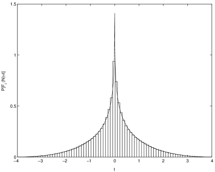
Figure 2. Scaled distribution of normalized matrix elements $F_{i}(\vec{n})=N\langle T_{N}(\vec{n})\phi_{i},\phi_{i}\rangle\;,\;\vec{n}=(1,1,0,0)\not\in Z_{1}\cup Z_{2}$ for $N=1613$. Plotted together the corresponding distribution $y(t)=\frac{1}{2\pi^{2}}\int_{t/2}^{2}\sqrt{(4-s^{2})(4-(\frac{s}{t})^{2})}\frac{ds}{s}$

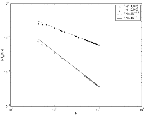
Figure 3. The values of $\max_{i}|\langle T_{N}(\vec{n})\phi_{i},\phi_{i}\rangle|$ for $\vec{n}=(1,0,0,0),(1,1,0,0)$ and values of N between 100 and 1000. Plotted together with the predicted decay of $2N^{-0.5},4N^{-1}$ respectively, on a log-log scale.

References

- [1] F. Bonechi, and S. De Bièvre Controlling strong scarring for quantized ergodic toral automorphisms, Duke Math. J. 117(3) (2003), 571–587.
- [2] A. Bouzouina, and S. De Bièvre Equipartition of the eigenfunctions of quantized ergodic maps on the torus, Commun. Math. Phys. 178 (1996), 83–105.
- [3] S. De Bièvre, and M. Degli Esposti Egorov theorems and equidistribution of eigenfunctions for the quantized sawtooth and Baker maps, Ann. Inst. Poincaré 69 (1998), 1–30.
- [4] M. Degli Esposti and S. Graffi Mathematical aspects of quantum maps, The mathematical aspects of quantum maps (M. Degli Esposti and S. Graffi, eds.), Lecture Notes in Physics, vol. 618, Springer,Berlin, 2003, pp. 49–90.
- [5] B.Eckhardt, S.Fishman, J. Keating, O. Agam, J. Main, and K. Müller, Approach to ergodicity in quantum wave functions., Phys. Rev. E 52(6) (1995), 5893–5903.
- [6] F. Faure, S. Nonnenmacher and S. De Bièvre, Scarred eigenstates for quantum cat maps of minimal periods, comm. Math. Phys. 239(3) (2003), 449–492.
- [7] M.Feingold and A.Peres, Distribution of matrix elements of chaotic systems, Phys. Rev. A 34(1) (1986), 591–595.
- [8] S. Gurevich and R. Hadani , Proof of the Kurlberg-Rudnick Rate Conjecture., preprint 2004, arXiv:math–ph/0404074 .
- [9] J.H. Hanny and M.V. Berry, Quantization of linear maps on a torus-Fresnel diffraction by a periodic grating, Phys.D 1 (1980), 267–290.
- [10] H. Iwaniec, Spectral Methods of Automorphic Forms , Graduate Studies in Mathematics 53, American Mathematical Society, Rhode Islans, 2002.
- [11] J.P. Keating and N.C. Snaith Random matrix theory and L-functions at s=1/2., Comm. Math. Phys. 214(1) (2000), 91–110.
- [12] D. Kelmer , Hecke theory for the cat map on the multidimensional torus, PhD Thesis Tel-Aviv University –in preparation.
- [13] S. Knabe On the quantisation of Arnold’s cat, J.Phys. A: Math. Gen. 23 (1990), 2013–2025.
- [14] A. Knauf Introduction to dynamical systems , The mathematical aspects of quantum maps (M. Degli Esposti and S. Graffi, eds.), Lecture Notes in Physics, vol. 618, Springer,Berlin, 2003, pp. 1–24.
- [15] P. Kurlberg and Z. Rudnick, Hecke theory and equidistribution for the quantization of linear maps of the torus, Duke math. J. 103(1) (2000), 47–77.
- [16] P.Kurlberg and Z. Rudnick, On the distribution of matrix elements for the quantum cat map, Ann. of Math. 161 (2005), 1-19.
- [17] W. Z. Luo and P. Sarnak, Quantum variance for Hecke eigenforms –In preparation.
- [18] J. M. Robbins T. O. de Carvalho, J. Keating, Fluctuations in quantum expectation values for chaotic systems with broken time-reversal symmetry, J. Phys. A:Math. Gen 31 (1998), 5631–5640.
- [19] A.I Šhnirel’man, Ergodic properties of eigenfunctions, Usp. Mat. Nauk 29 (1974), 181–182.
- [20] S. Zelditch, Uniform distribution of eigenfunctions om compact hyperbolic surfaces, Duke Math. J. 55(4) (1987), 919–941.