Orthogonal polynomials with discontinuous weights

Abstract

In this paper we present a brief description of a ladder operator formalism applied to orthogonal polynomials with discontinuous weights. The two coefficient functions, $A_{n}(z)$ and $B_{n}(z)$, appearing in the ladder operators satisfy the two fundamental compatibility conditions previously derived for smooth weights. If the weight is a product of an absolutely continuous reference weight $w_{0}$ and a standard jump function, then $A_{n}(z)$ and $B_{n}(z)$ have apparent simple poles at these jumps. We exemplify the approach by taking $w_{0}$ to be the Hermite weight. For this simpler case we derive, without using the compatibility conditions, a pair of difference equations satisfied by the diagonal and off-diagonal recurrence coefficients for a fixed location of the jump. We also derive a pair of Toda evolution equations for the recurrence coefficients which, when combined with the difference equations, yields a particular Painlevé IV.

1 Introduction

We begin this section by fixing the notation. Let $P_{n}(x)$ be monic polynomials of degree $n$ in $x$ and orthogonal, with respect to a weight, $w(x),\;x\in[a,b]$,

$$\int_{a}^{b}P_{m}(x)P_{n}(x)w(x)dx=h_{n}\delta_{m,n}\ ,$$ (1)

where $h_{n}$ is the square of the weighted $L^{2}$ norm of $P_{n}.$ Also,

$$P_{n}(z)=z^{n}+{\mathsf{p}_{1}}(n)z^{n-1}+\dots\ .$$ (2)

For convenience we set $w(a)=w(b)=0$. The recurrence relation follows from the orthogonality condition:

$$zP_{n}(z)=P_{n+1}(z)+\alpha_{n}P_{n}(z)+\beta_{n}P_{n-1}(z)\quad n=0,1,...\ ,$$ (3)

where $\beta_{0}P_{-1}(z):=0$, the $\alpha_{n},\;n=0,1,2,\dots$ are real and $\beta_{n},\;n=1,2,\dots$ are strictly positive.

In this paper we describe a formalism which will facilitate the determination of the recurrence coefficients for polynomials with singular weights. Two points of view lead to this problem: On one hand the X-ray problem [1] of condensed matter theory, on the other hand related problems in random matrix theory which involve the asymptotics of the Fredholm determinant of finite convolution operators with discontinuous symbols [8]. This paper is the first in a series that systematically study orthogonal polynomial where the otherwise smooth weights have been singularly deformed. The ultimate aim is the computation for large $n$ of the determinant $D_{n}$ of the $n\times n$ moments or Hankel matrix $(\mu_{j+k})_{j,k=0}^{n-1}$ with moments $\mu_{j}:=\int_{a}^{b}w(t)t^{j}dt$ where $j=0,1,\dots$, thereby doing what has been done for the determinants of $n\times n$ Toeplitz matrices with singular generating functions [2].

The deformed weight with one jump is

$$w(x)=w_{0}(x)\left(1-\frac{\beta}{2}+\beta\theta(x-{\tilde{x}})\right)\ ,$$ (4)

where $a<{\tilde{x}}<b$ is the position of the jump, $\theta(.)$ is the Heaviside step function and the real $\beta$ parametrises the height of the jump. More generally, we take $w_{{\mathsf{J}}}>0$ to be the canonical jump function $w_{{\mathsf{J}}}(x)=1+\sum_{j=1}^{\mathcal{N}}\Delta_{j}\theta(x-{\tilde{x}}_{j})$ and $w(x):=w_{0}(x)w_{J}(x)$.

The actions of the ladder operators on $P_{n}(z)$ and $P_{n-1}(z)$ are

$$\left(\frac{d}{dz}+B_{n}(z)\right)P_{n}(z) = \beta_{n}A_{n}(z)P_{n-1}(z)$$ (5)

$$\left(\frac{d}{dz}-B_{n}(z)-{\mathsf{v}}_{0}^{\prime}(z)\right)P_{n-1}(z) = -A_{n-1}(z)P_{n}(z)$$ (6)

$$A_{n}(z):=\sum_{j=1}^{\mathcal{N}}\frac{R_{n}(j)}{z-{\tilde{x}}_{j}}+\frac{1}{h_{n}}\int_{a}^{b}\frac{{\mathsf{v}}_{0}^{\prime}(z)-{\mathsf{v}}_{0}^{\prime}(y)}{z-y}P_{n}^{2}(y)w(y)dy$$ (7)

$$B_{n}(z):=\sum_{j=1}^{\mathcal{N}}\frac{r_{n}(j)}{z-{\tilde{x}}_{j}}+\frac{1}{h_{n-1}}\int_{a}^{b}\frac{{\mathsf{v}}_{0}^{\prime}(z)-{\mathsf{v}}_{0}^{\prime}(y)}{z-y}P_{n-1}(y)P_{n}(y)w(y)dy$$ (8)

where $w_{0}(x)=:\exp(-{\mathsf{v}}_{0}(x))$. If $w(a)$ and $w(b)$ are non-vanishing one must add

$$\left.\frac{P_{n}^{2}(y)w(y)}{h_{n}(y-z)}\right|_{y=a}^{b}\quad\textrm{and}\quad\left.\frac{P_{n}(y)P_{n-1}(y)w(y)}{h_{n-1}(y-z)}\right|_{y=a}^{y=b}$$

to (7) and (8) respectively.

Now $A_{n}(z)$ and $B_{n}(z)$, the coefficient functions in the ladder operators, satisfy identities analogous to those found for smooth weights [5, 7, 4]:

$$B_{n+1}(z)+B_{n}(z) = (z-\alpha_{n})A_{n}(z)-{\mathsf{v}}_{0}^{\prime}(z)$$ (9)

$$B_{n+1}(z)-B_{n}(z) = \frac{\beta_{n+1}A_{n+1}(z)-\beta_{n}A_{n-1}(z)-1}{z-\alpha_{n}}$$ (10)

$$R_{n}({\tilde{x}}_{j})=R_{n}(\Delta_{1},...,\Delta_{\mathcal{N}},{\tilde{x}}_{j}) := \frac{\Delta_{j}}{h_{n}}P_{n}^{2}({\tilde{x}}_{j})w_{0}({\tilde{x}}_{j})$$ (11)

$$r_{n}({\tilde{x}}_{j})=r_{n}(\Delta_{1},...,\Delta_{\mathcal{N}},{\tilde{x}}_{j}) := \frac{\Delta_{j}}{h_{n-1}}P_{n}({\tilde{x}}_{j})P_{n-1}({\tilde{x}}_{j})w_{0}({\tilde{x}}_{j})$$ (12)

The derivation of (5)-(12) will be published in a forthcoming paper where the weight has several jumps and $w_{0}(x)=(1-x)^{\alpha}(1+x)^{\beta},\;\;x\in[-1,1]$ is the Jacobi weight.

Multiplying the recurrence relation (3) evaluated at $z={\tilde{x}}_{j}$ by $\Delta_{j}w_{0}({\tilde{x}}_{j})P_{n}({\tilde{x}}_{j})$ and noting (11) as well as (12) we arrive at the universal equality

$$({\tilde{x}}_{j}-\alpha_{n})R_{n}({\tilde{x}}_{j})=r_{n+1}({\tilde{x}}_{j})+r_{n}({\tilde{x}}_{j})\ .$$ (13)

Similarly, squaring $r_{n}({\tilde{x}}_{j})$ we find a second universal equation

$$r_{n}^{2}({\tilde{x}}_{j})=\beta_{n}R_{n}({\tilde{x}}_{j})R_{n-1}({\tilde{x}}_{j})\ .$$ (14)

Note that in the expressions for $A_{n}(z)$ and $B_{n}(z)$ only ${\mathsf{v}}_{0}$, the “potential” associated with the smooth reference weight, appears. The discontinuities give rise to $R_{n}({\tilde{x}}_{j})$ and $r_{n}({\tilde{x}}_{j}).$

It is clear from (7) and (8) that if ${\mathsf{v}}_{0}^{\prime}(z)$ is rational, then $A_{n}(z)$ and $B_{n}(z)$ are also rational. This is particularly useful for our purpose which is the determination of the recurrence coefficients, for in this situation by comparing residues on both sides of (9) and (10) we should find the required difference equations [4].

In the following section the above approach is exemplified by the Hermite weight, $w_{0}(x)=\exp(-x^{2})$ and $w$ given by (4). It turns out that in this situation $\alpha_{n}$ and $\beta_{n}$ are related to $R_{n}$ and $r_{n}$ in a very simple way.

2 Hermite weight with one jump

Now, $w_{0}(x)=\exp(-x^{2})$, so that ${\mathsf{v}}_{0}(x)=x^{2}$, and $w(x)$ as in (4). Also,

$$R_{n} := R_{n}({\tilde{x}})=\beta\frac{P_{n}^{2}({\tilde{x}},{\tilde{x}})}{h_{n}({\tilde{x}})}w_{0}({\tilde{x}})$$ (15)

$$r_{n} := r_{n}({\tilde{x}})=\beta\frac{P_{n}({\tilde{x}},{\tilde{x}})P_{n-1}({\tilde{x}},{\tilde{x}})}{h_{n-1}({\tilde{x}})}w_{0}({\tilde{x}})\ ,$$ (16)

which are independent of the particular choice of $w_{0}$ and

$$A_{n}(z)=\frac{R_{n}}{z-{\tilde{x}}}+2\quad\textrm{and}\quad B_{n}(z)=\frac{r_{n}}{z-{\tilde{x}}}\ ,$$ (17)

particular to ${\mathsf{v}}_{0}(x)=x^{2}.$ Note that $P_{j}({\tilde{x}},{\tilde{x}})$ is the value of $P_{j}(z,{\tilde{x}})$ at $z={\tilde{x}}.$

Instead of proceeding with the full machinery of (9) and (10) we take advantage of the fact that ${\mathsf{v}}_{0}(x)=x^{2}$. From orthogonality and the recurrence relation, we have

$$\alpha_{n}({\tilde{x}})h_{n}({\tilde{x}})=\frac{1}{2}\int_{-\infty}^{\infty}{\mathsf{v}}_{0}^{\prime}(x)P^{2}_{n}(x,{\tilde{x}})w(x)dx=\frac{R_{n}({\tilde{x}})}{2}h_{n}({\tilde{x}})$$ (18)

by integration by parts. The string equation,

$$nh_{n-1}({\tilde{x}})=\int_{-\infty}^{\infty}P_{n}^{\prime}(x,{\tilde{x}})P_{n-1}(x,{\tilde{x}})w(x)dx\ ,$$ (19)

is an immediate consequence of the orthogonality condition. Again, an integration by parts and noting that $\beta_{n}=h_{n}/h_{n-1}$ produces

$$\beta_{n}({\tilde{x}})=\frac{n}{2}+\frac{r_{n}({\tilde{x}})}{2}\ .$$ (20)

It should be pointed out here that in general neither the string equation (19) nor (18) will provide the complete set of difference equations for the recurrence coefficients which can be seen if $w_{0}$ were the Jacobi weight. In such a situation the compatibility conditions (9) and (10) must be used.

Now (13) and (14) become

$$\frac{r_{n+1}+r_{n}}{2}=\alpha_{n}({\tilde{x}}-\alpha_{n})\ .$$ (21)

and

$$r_{n}^{2}=2(n+r_{n})\alpha_{n}\alpha_{n-1}\ .$$ (22)

Equations (21) and (22), supplemented by the initial conditions

$$\alpha_{0}({\tilde{x}})=\frac{\beta}{2}\exp(-{\tilde{x}}^{2})\left[(1-\beta/2)\sqrt{\pi}+\beta\int_{{\tilde{x}}}^{\infty}\exp(-t^{2})dt\right]^{-1}\quad\textrm{and}\quad r_{0}({\tilde{x}})=0\ ,$$

can be iterated to determine the recurrence coefficients numerically. Also, explicit solutions to (21) and (22) can be produced for small $n$.

3 Derivative with respect to ${\tilde{x}}$ and Painlevé IV

If (21) and (22) are combined with the evolution equations to be derived in this section, the Painlevé IV mentioned in the abstract is found. We begin with the $L^{2}$ norm $h_{n}({\tilde{x}})$, Equation (1), which entails

$$\partial_{{\tilde{x}}}h_{n}=-\beta\int_{-\infty}^{\infty}P_{n}^{2}(x)w_{0}(x)\delta(x-{\tilde{x}})dx=-\beta P_{n}^{2}({\tilde{x}})w_{0}({\tilde{x}})=-h_{n}R_{n}=-2h_{n}\alpha_{n}\ .$$ (23)

and thus $\partial_{{\tilde{x}}}\ln\beta_{n}=-2(\alpha_{n}-\alpha_{n-1})$ since $\ln\beta_{n}=\ln h_{n}-\ln h_{n-1}$. With (20),

$$\frac{1}{2(n+r_{n})}{\partial_{{\tilde{x}}}}r_{n}=\alpha_{n-1}-\alpha_{n}$$ (24)

which is the first Toda equation. Taking the derivative with respect to ${\tilde{x}}$ of (1) at $m=n-1$ and using the definition of the monic polynomials (2) then gives $\partial_{{\tilde{x}}}{\mathsf{p}_{1}}(n,{\tilde{x}})=r_{n}$ since ${\mathsf{p}_{1}}(n,{\tilde{x}})-{\mathsf{p}_{1}}(n+1,{\tilde{x}})=\alpha_{n}({\tilde{x}})$ is an immediate consequence of the recurrence relation. Therefore

$$\partial_{{\tilde{x}}}\alpha_{n}=r_{n}-r_{n+1}\ ,$$ (25)

the second Toda equation.

Eliminating $r_{n+1}$ from (21) and the second Toda equation (25), gives $r_{n}$ in terms of $\alpha_{n}$ and ${\partial_{{\tilde{x}}}}\alpha_{n}$:

$$r_{n}=\alpha_{n}({\tilde{x}}-\alpha_{n})+\frac{1}{2}{\partial_{{\tilde{x}}}}\alpha_{n}\ .$$ (26)

Using the first Toda equation (24) to express $\alpha_{n-1}$ in terms of $\alpha_{n}$ and ${\partial_{{\tilde{x}}}}r_{n}$ and substituting (26) into (22) produces a particular Painlevé IV [3],

$$\alpha_{n}^{\prime\prime}=\frac{(\alpha_{n}^{\prime})^{2}}{2\alpha_{n}}+6\alpha_{n}^{3}-8{\tilde{x}}\alpha_{n}^{2}+2({\tilde{x}}^{2}-(2n+1))\alpha_{n}\ ,$$ (27)

which can be brought into the canonical form with the replacements $\alpha_{n}\to\alpha_{n}/2$ and ${\tilde{x}}\to-{\tilde{x}}$. Equation (27) is supplemented by the boundary conditions $\lim_{{\tilde{x}}\to\pm\infty}\alpha_{n}({\tilde{x}})=0$. In a recent paper [6], a Painlevé IV was derived for the discontinuous Hermite weight using an entirely different method.

Based on (23) and (25) the derivative of the logarithm of the Hankel determinant $D_{n}=\prod_{j=0}^{n-1}h_{j}$ can be computed as

$$\partial_{{\tilde{x}}}\ln D_{n} = -2\sum_{j=0}^{n-1}\alpha_{j}=-\sum_{j=0}^{n-1}R_{j}=-\beta\exp(-{\tilde{x}}^{2})\sum_{j=0}^{n-1}\frac{P_{j}^{2}({\tilde{x}},{\tilde{x}})}{h_{j}({\tilde{x}})}$$ (28)

$$\partial_{{\tilde{x}}}^{2}\ln D_{n} = 2r_{n}\ .$$ (29)

where (15) has been used in the first line, which can be summed by the Christoffel-Darboux formula,

$$\sum_{j=0}^{n-1}\frac{P_{j}(x,{\tilde{x}})P_{j}(y,{\tilde{x}})}{h_{j}({\tilde{x}})}=\frac{P_{n}(x,{\tilde{x}})P_{n-1}(y,{\tilde{x}})-P_{n}(y,{\tilde{x}})P_{n-1}(x,{\tilde{x}})}{(x-y)h_{n-1}({\tilde{x}})}\ .$$

In the limit $x\to y,$ we find, in general,

$$h_{n-1}({\tilde{x}})\sum_{j=0}^{n-1}\frac{P_{j}^{2}(x,{\tilde{x}})}{h_{j}({\tilde{x}})}$$

$$=\beta_{n}A_{n}(x)P_{n-1}^{2}(x,{\tilde{x}})+A_{n-1}(x)P_{n}^{2}(x,{\tilde{x}})-\big{(}2B_{n}(x)+{\mathsf{v}}_{0}^{\prime}(x)\big{)}P_{n}(x,{\tilde{x}})P_{n-1}(x,{\tilde{x}})$$

using the the ladder operators (5) and (6). With (17) this entails

$$\sum_{j=0}^{n-1}\frac{P_{j}^{2}(x,{\tilde{x}})}{h_{j}({\tilde{x}})}=\frac{1}{h_{n-1}({\tilde{x}})}\left(2\beta_{n}P_{n-1}^{2}(x,{\tilde{x}})+2P_{n}^{2}(x,{\tilde{x}})-2xP_{n}(x,{\tilde{x}})P_{n-1}(x,{\tilde{x}})\right)$$

$$\qquad+\frac{1}{(x-{\tilde{x}})h_{n-1}({\tilde{x}})}\left(\beta_{n}R_{n}P_{n-1}^{2}(x,{\tilde{x}})+R_{n-1}P_{n}^{2}(x,{\tilde{x}})-2r_{n}P_{n}(x,{\tilde{x}})P_{n-1}(x,{\tilde{x}})\right)$$

The apparent pole at $x={\tilde{x}}$ can be shown to have vanishing residue by considering $\beta\exp(-{\tilde{x}}^{2})\times(\textrm{residue})$:

$$\beta\exp(-{\tilde{x}}^{2})\Big{(}\beta_{n}R_{n}P_{n-1}^{2}({\tilde{x}},{\tilde{x}})+R_{n-1}P_{n}^{2}({\tilde{x}},{\tilde{x}})-2r_{n}P_{n}({\tilde{x}},{\tilde{x}})P_{n-1}({\tilde{x}},{\tilde{x}})\Big{)}/h_{n-1}$$

$$=2(n+r_{n})\alpha_{n}\alpha_{n-1}+2(n+r_{n})\alpha_{n-1}\alpha_{n}-2r_{n}^{2}=2\big{(}2(n+r_{n})\alpha_{n}\alpha_{n-1}-r_{n}^{2}\big{)}=0 \ ,$$

where the last equality is due to (22). A further regular term can be found as a contribution from the Taylor series of $P_{j}(x,{\tilde{x}})$ about $x={\tilde{x}}$ namely,

$$2\frac{\beta_{n}}{h_{n-1}}R_{n}P_{n-1}({\tilde{x}},{\tilde{x}})P_{n-1}^{\prime}({\tilde{x}})+2\frac{R_{n-1}}{h_{n-1}}P_{n}({\tilde{x}},{\tilde{x}})P_{n}^{\prime}({\tilde{x}})$$

$$-2\frac{r_{n}}{h_{n-1}}\partial_{x}\left.\left(P_{n-1}(x,{\tilde{x}})P_{n}(x,{\tilde{x}})\right)\right|_{x={\tilde{x}}}$$ (30)

where $P_{j}^{\prime}({\tilde{x}}):={\partial_{{\tilde{x}}}}P_{j}(x,{\tilde{x}})|_{x={\tilde{x}}}$. Using the fact that $\beta_{n}=h_{n}/h_{n-1}$ and (15), we see that the first two terms of (30) combined into $2(r_{n}/h_{n-1})\partial_{x}(P_{n}(x,{\tilde{x}})P_{n-1}(x,{\tilde{x}}))|_{x={\tilde{x}}}$ cancel the third. We are therefore left with the regular term:

$${\partial_{{\tilde{x}}}}\ln D_{n}=-\beta\left(2\beta_{n}\frac{P_{n-1}^{2}({\tilde{x}},{\tilde{x}})}{h_{n-1}}+2\frac{P_{n}^{2}({\tilde{x}},{\tilde{x}})}{h_{n-1}}-2{\tilde{x}}\frac{P_{n}({\tilde{x}},{\tilde{x}})P_{n-1}({\tilde{x}},{\tilde{x}})}{h_{n-1}}\right)\exp(-{\tilde{x}}^{2})$$

$$=2{\tilde{x}}r_{n}-2(n+r_{n})(\alpha_{n}+\alpha_{n-1})\ .$$ (31)

Using (24)–(26) it follows from $2{\tilde{x}}r_{n}^{\prime}-2r_{n}^{\prime}(\alpha_{n}+\alpha_{n-1})-2(n+r_{n})(\alpha_{n}^{\prime}+\alpha_{n-1}^{\prime})=4(n+r_{n})\left(r_{n-1}-r_{n}-\alpha_{n-1}^{\prime}\right)=0$ that (31) reproduces the second derivative (29), $\partial_{{\tilde{x}}}^{2}\ln D_{n}=2r_{n}$.

Let $F_{n}({\tilde{x}}):=-\ln D_{n}({\tilde{x}})$ be the free energy. Expressing (31) in terms of $\alpha_{n}({\tilde{x}})$ and finally in terms of $\Psi_{n}({\tilde{x}})$, where $\alpha_{n}({\tilde{x}})=:\frac{\beta}{2}(\Psi_{n}({\tilde{x}}))^{2}$, the free energy reads

$$F_{n}({\tilde{x}})-F_{n}(-\infty) = \frac{\beta}{2}\int_{-\infty}^{{\tilde{x}}}\left((4n+1-2x^{2})\Psi_{n}^{2}(x)+3\beta x\Psi_{n}^{4}(x)-\beta^{2}\Psi^{6}_{n}(x)\right)dx$$

$$+\frac{\beta}{2}\Psi_{n}({\tilde{x}})\Psi_{n}^{\prime}({\tilde{x}})\ ,$$

where $F_{n}(-\infty)$ is the free energy corresponding to $w(x)=\exp(-x^{2})$. Note that $\exp(-F_{n}(\pm\infty))=2\pi^{n/2}\prod_{k=1}^{n}\frac{\Gamma(k)}{2^{k}}$, which gives rise to the sum rule

$$\int_{-\infty}^{\infty}\Big{(}(4n+1-2x^{2})\Psi_{n}^{2}(x)+3\beta x\Psi_{n}^{4}(x)-\beta^{2}\Psi^{6}_{n}(x)\Big{)}dx=0\ .$$

With a minor change of variables (29) becomes the Toda molecule equation. First we note that

$$r_{n}({\tilde{x}})=2\beta_{n}({\tilde{x}})-n\quad\textrm{and}\quad\beta_{n}({\tilde{x}})=\frac{h_{n}({\tilde{x}})}{h_{n-1}({\tilde{x}})}=\frac{D_{n+1}({\tilde{x}})D_{n-1}({\tilde{x}})}{(D_{n}({\tilde{x}}))^{2}}\ .$$

Defining $D_{n}({\tilde{x}})=:\exp(-n{\tilde{x}}^{2}){\tilde{D}}_{n}({\tilde{x}})$ it then follows

$${\partial_{{\tilde{x}}}}^{2}\ln{\tilde{D}}_{n}=4\frac{{\tilde{D}}_{n+1}{\tilde{D}}_{n-1}}{({\tilde{D}}_{n})^{2}}\ .$$

We may express $\alpha_{n}({\tilde{x}})$ in terms of the derivatives of the free energy, by noting that $-F_{n}^{\prime}=2{\tilde{x}}r_{n}-2(n+r_{n})(\alpha_{n}+\alpha_{n-1})$ and $-F_{n}^{\prime\prime}=2r_{n}$. One finds with (24)

$$\alpha_{n}({\tilde{x}})=\frac{F_{n}^{\prime}-{\tilde{x}}F_{n}^{\prime\prime}+F_{n}^{\prime\prime\prime}/2}{4n-2F_{n}^{\prime\prime}}=\frac{{\tilde{x}}}{2}-\frac{1}{4}\frac{f_{n}^{\prime\prime\prime}+2f_{n}^{\prime}}{f_{n}^{\prime\prime}}$$

where $F_{n}({\tilde{x}})=:f_{n}({\tilde{x}})+n{\tilde{x}}^{2}$.

4 Asymptotics and Numerics

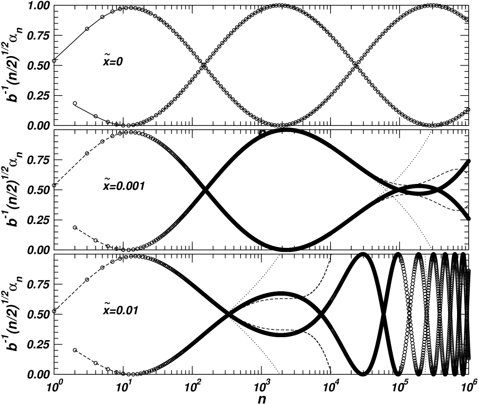
Figure 1: Behaviour of $b^{-1}(n/2)^{1/2}\alpha_{n}$ for $\beta=3/2$ and various (small) values of ${\tilde{x}}$ from a numerical iteration of (21) and (22). The top panel shows additionally Equation (4) as a solid line passing through the open circles. The other two panels show the approximation of the rescaled $\alpha_{n}({\tilde{x}})$ using the first three (two) terms of a Taylor series around ${\tilde{x}}=0$ as dashed (dotted) line. The behaviour of $r_{n}$ looks likewise. The numerical data is pruned differently in the three cases to avoid artefacts.

For ${\tilde{x}}=0$ we find the asymptotic expansion

$$\alpha_{n}(0) = \frac{b}{\sqrt{2n}}\Big{[}1+(-1)^{n}\sin(2b\ln n+B)$$

$$-\frac{1}{4n}\big{(}1+(-1)^{n}(\sin(2b\ln n+B)-4b\cos(2b\ln n+B))\big{)}+\mathcal{O}(n^{-2})\Big{]}$$

$$r_{n}(0) = -b(-1)^{n}\cos(2b\ln n+B)-\frac{b^{2}}{2n}\Big{(}1+\sin^{2}(2b\ln n+B)\Big{)}+\mathcal{O}(n^{-2})$$ (33)

guided by the numerics on the difference equations (21) and (22). The constant $b$ is given by

$$b:=\frac{1}{2\pi}\ln\left(\frac{1+\beta/2}{1-\beta/2}\right)\quad\textrm{with}\quad\frac{\beta}{2}\in(-1,1)$$

and $B$ is a phase independent of $n$. Unfortunately, the formalism developed in this paper does not seem to shed any light on its delicate dependence on $\beta$.

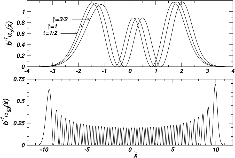
Figure 2: Upper panel: $b^{-1}\alpha_{2}({\tilde{x}})$ for different jump heights $\beta$ as a function of ${\tilde{x}}$. Lower panel: For large $n$ the rescaled coefficient $b^{-1}\alpha_{50}({\tilde{x}})$ fluctuates wildly.

It can be verified by a direct calculation that (4) and (33) satisfy (21) and (22) to order $1/n^{2}$. The top panel of figure 1 shows a comparison between the numerical results and the above asymptotes for suitably rescaled $\alpha_{n}$. In principle, $\alpha_{n}$ and $r_{n}$ can be determined analytically to any order in $n$ because an approximation of $\alpha_{n}$ to order $n^{-m}$ gives rise to a difference equation for $r_{n}$ to order $n^{-(m+1)}$ via (21). In turn, $r_{n}$ to order $n^{-(m+1)}$ produces an equation for $\alpha_{n}$ to order $n^{-(m+1)}$ and so forth. This scheme breaks down for ${\tilde{x}}\neq 0$.

For fixed ${\tilde{x}}\neq 0$, the numerics does not suggest an ansatz for the asymptotes. Most remarkably, the effect of ${\tilde{x}}\neq 0$ persists for very large $n$, even for very small ${\tilde{x}}\neq 0$, as illustrated in figure 1. Also shown in this figure as dashed (dotted) lines are the approximations of $\alpha_{n}({\tilde{x}})$ from the first three (two) terms of a Taylor-series in ${\tilde{x}}$ around ${\tilde{x}}=0$ based on the iterative results for $\alpha_{n}({\tilde{x}}=0)$, (25) and (27). In principle, the Painlevé IV, Equation (27), provides a way to express $\alpha_{n}^{(m)}({\tilde{x}})$ in terms of lower order derivatives $\alpha_{n}^{(m^{\prime})}({\tilde{x}})$ with $m^{\prime}<m$, yet the results in figure 1 suggest that for sufficiently large $n$ a finite Taylor series eventually deviates wildly from the correct $\alpha_{n}({\tilde{x}})$. Note that both $\sqrt{n}\alpha_{n}({\tilde{x}})$ and $r_{n}({\tilde{x}})$ are bounded in $n$ for large $n$.

Figure 2 shows the rescaled $\alpha_{n}$ for fixed $n$ and varying ${\tilde{x}}$. It resembles a Hermite polynomial because of its direct relation to $P_{n}^{2}({\tilde{x}},{\tilde{x}})w_{0}({\tilde{x}})$, (18) and (15). For the same reason $\alpha_{n}({\tilde{x}})$ vanishes for $n\ln({\tilde{x}})\ll{\tilde{x}}^{2}/2$.

References

References

[1] E. L. Basor and Y. Chen, “The X-ray problem revisited”,
J. Phys. A.: Math. Gen. 36 (2003) L175-L180; “A note on the Wiener-Hopf
determinants and the Borodin-Okunkov identity”, Integr. Equ. Oper. Theory,
45 (2003) 301-308.
[2] H. Widom, “Toeplitz determinants with singular generating
functions”,
Amer. J. Math., 95 (1973) 333-383; E. L. Basor, “Asymptotic formulas
for Toeplitz determinants”, Trans. Amer. Math. Soc. 239 (1978) 33-65.
[3] A. P. Bassom, P. A. Clarkson, A. C. Hicks, and J. B.
McLeod, “Integral equations and exact solutions of the fourth Painlevé
equation”,
Proc. R. Soc. London Ser. A 437 (1992) 1-24.
[4] Y. Chen and M. E. H. Ismail, “Jacobi polynomials from compatibility
conditions”, Proc. Amer. Math. Soc. 133 (2005) 465-472,
225-237.
[5]Y. Chen and M. E. H. Ismail, “Ladder operators
and differential equations for orthogonal polynomials”,
J. Phys. A.: Math. Gen. 30 (1997) 7817-7829.
[6] P. J. Forrester and N. S. Witte, “Discrete Painlevé
equations and random matrix averages”, Nonlinearity, 16 (2003)
1919-1944.
[7]M. E. H. Ismail and J. Wimp, “On differential
equations for orthogonal polynomials”, Methods Appl. Anal.
5 (1998) 439-452.
[8]M. Jimbo, T. Miwa, Y. Môri and M. Sato, “Density
matrix of an impenetrable Bose gas and the fifth Painlevé transcendent”, Physica D 1 (1980) 80–158.