Pushmepullyou: An efficient micro-swimmer

Abstract

The swimming of a pair of spherical bladders that change their volumes and mutual distance is efficient at low Reynolds numbers and is superior to other models of artificial swimmers. The change of shape resembles the wriggling motion known as metaboly of certain protozoa.

Swimming at low Reynolds numbers can be remote from common intuition because of the absence of inertia [1]. In fact, even the direction of swimming may be hard to foretell [2]. At the same time, and not unrelated to this, it does not require elaborate designs: Any stroke that is not self-retracing will, generically, lead to some swimming [3]. A simple model that illustrates these features is the three linked spheres [4], Fig. 1 (right), that swim by manipulating the distances $\ell_{1,2}$ between neighboring spheres. The swimming stroke is a closed, area enclosing, path in the $\ell_{1}-\ell_{2}$ plane. Another mechanical model that has actually been built is Purcell’s two hinge model [5].

Swimming efficiently is an issue for artificial micro-swimmers [6]. As we have been cautioned by Purcell not to trust common intuition at low Reynolds numbers [2], one may worry that efficient swimming may involve unusual and nonintuitive swimming styles. The aim of this letter is to give an example of an elementary and fairly intuitive swimmer that is also remarkably efficient provided it is allowed to make large strokes.

The swimmer is made of two spherical bladders, Fig. 1 (left). The bladders are elastic bodies which impose no-slip boundary conditions. The device swims by cyclically changing the distance between the bladders and their relative volumes. For the sake of simplicity and concreteness we assume that their total volume, $v_{0}$, is conserved. The swimming stroke is a closed path in the $v-\ell$ plane where $v$ is the volume of, say, the left sphere and $\ell$ the distance between them. We shall make the further simplifying assumption that the viscosity of the fluid contained in the bladders is negligible compared with the viscosity of the ambient fluid. For reasons that shall become clear below we call the swimmer pushmepullyou.

Like the three linked spheres, pushmepullyou is mathematically elementary only in the limit that the distance between the spheres is large, i.e. when $\varepsilon_{i}=a_{i}/\ell\ll 1$. ($a_{i}$ stands for the radii of the two spheres and $\ell$ for the distances between the spheres.) We assume that the Reynolds number $R={\rho av/\mu}\ll 1$, and that the distance $\ell$ is not too large: ${\ell v}\ll\mu/\rho$. The second assumption is not essential and is made for simplicity only. (To treat large $\ell$ one needs to replace the Stokes solution, Eq. (11), by the more complicated, but still elementary, Oseen-Lamb solution [7].)

Pushmepullyou is simpler than the three linked spheres: It involves two spheres rather than three; it is more intuitive and is easier to solve mathematically. It also swims a larger distance per stroke and is considerably more efficient [8]. If large strokes are allowed, it can even outperform conventional models of biological swimmers that swim by beating a flagellum [9]. If only small strokes are allowed then pushmepullyou, like all squirmers [6], becomes rather inefficient.

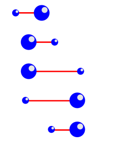
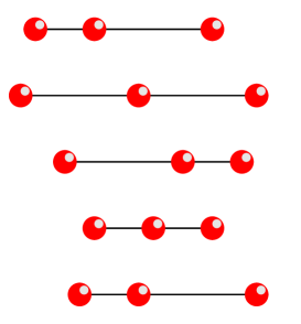
Figure 1: Five snapshots of the pushmepullyou swimming stroke (left) and the corresponding strokes of the three linked spheres (right). Both figures are schematic. After a full cycle the swimmers resume their original shape but are displaced to the right. Pushmepullyou is both more intuitive and more efficient than the three linked spheres.

The swimming velocity is defined by $\dot{X}=(U_{1}+U_{2})/2$ where $U_{i}$ are the velocities of the centers of the two spheres. To solve a swimming problem one needs to find the (linear) relation between the (differential) displacement $\kern-1.00006pt{\raise 3.44444pt\hbox{ -}}\kern-6.00006pt{d}X$, and the (differential) controls $(d\ell,dv)$. This relation, as we shall show, takes the form:

$$2\,\kern-1.00006pt{\raise 3.44444pt\hbox{ -}}\kern-6.00006pt{d}X=\frac{a_{1}-a_{2}}{a_{1}+a_{2}}\ d\ell\ +\frac{1}{2\pi\ell^{2}}\ dv,$$ (1)

where $a_{1},a_{2}$ are the radii of the left and right spheres respectively and $v$ is the volume of the left bladder. $\kern-1.00006pt{\raise 3.44444pt\hbox{ -}}\kern-6.00006pt{d}X$ stresses that the differential displacement does not integrate to a function $X(\ell,v)$. Rather, the displacement $X(\gamma)$ depends on the stroke $\gamma$, defined as a closed path in $\ell-v$ plane. The first term says that increasing $\ell$ leads to swimming in the direction of the small sphere. It can be interpreted physically as the statement that the larger sphere acts as an anchor while the smaller sphere does most of the motion when the “piston” $\ell$ is extended. The second term says that when $\ell$ is held fixed, the swimming is in the direction of the contracting sphere: The expanding sphere acts as a source pushing away the shrinking sphere which acts as a sink to pull the expanding sphere. This is why the swimmer is dubbed pushmepullyou.

To gain further insight consider the special case of small strokes near equal bi-spheres. Using Eq. (1) one finds, dropping sub-leading terms in $\varepsilon_{i}=a_{i}/\ell$:

$$\delta X=\,\frac{1}{6}\,d\log v\wedge d\ell$$ (2)

The distance covered in one stroke scales like the area in $\log v-\ell$ plane. Note that the swimming distance does not scale to zero with $\varepsilon$, when the spheres are far apart. This is in contrast with the three linked spheres where the swimming distance of one stroke is proportional to $\varepsilon$. For a small cycle in the $\ell_{1}-\ell_{2}$ plane Najafi et. al. find for a symmetric swimmer (Eq. (11) in [4]):

$$\delta X=0.7\varepsilon\,d\log\ell_{2}\wedge d\ell_{1}$$ (3)

When the swimmer is elementary, (=when $\varepsilon$ is small), it is also poor.

Consider now a large stroke associated with the closed rectangular path enclosing the box $\ell_{s}\leq\ell\leq\ell_{L},\;v_{s}\leq v_{1},v_{2}\leq v_{L}\equiv v_{0}-v_{s}$, where $v_{1}=v$ and $v_{2}$ are, respectively, the volumes of the left and right bladders. If $a_{s}\ll a_{L}$ then from Eq. (1), $X(\gamma)$ is essentially $\ell_{L}-\ell_{s}$:

$$X(\gamma)=\left(\frac{a_{L}-a_{s}}{a_{L}+a_{s}}\right)\ (\ell_{L}-\ell_{s})\left(1+O(\varepsilon^{3})\right)$$ (4)

This says that the distance covered in one stroke is of the order of the size of the swimmer, i.e. the distance between the balls $\ell$.

Certain protozoa and species of Euglena perform a wriggling motion known as metaboly where, like pushmepullyou, body fluids are transferred from a large spheroid to a small spheroid [10]. Metaboly is, at present not well understood and while some suggest that it plays a role in feeding others argue that it is relevant to locomotion [11]. The pushmepullyou model shows that at least as far as fluid dynamics is concerned, metaboly is a viable method of locomotion. Racing tests made by R. Triemer [12] show that Euglenoids swim 1-1.5 their body length per stroke, in agreement with Eq. (4) for reasonable choices of stroke parameters. Since Euglena resemble deformed pears — for which there is no known solution to the flow equations — Pushmepullyou is, at best, a biological over-simplification. It has the virtue that it admits complete analysis.

The second step in solving a swimming problem is to compute the power $P$ needed to propel the swimmer. By general principles, $P$ is a quadratic form in the velocities in the control space and is proportional to the (ambient) viscosity $\mu$. The problem is to find this quadratic form explicitly. If the viscosity of the fluid inside the bladders is negligible, one finds that in order to drive the controls $\ell$ and $v$, Pushmepullyou needs to invest the power

$$\frac{P}{6\pi\mu}=\left(\frac{1}{a_{1}}+\frac{1}{a_{2}}\right)^{-1}\,\dot{\ell}^{2}+\frac{2}{9\pi}\ \left(\frac{1}{v_{1}}+\frac{1}{v_{2}}\right)\dot{v}^{2}$$ (5)

Note that the dissipation associated with $\dot{\ell}$, is dictated by the small sphere and decreases as the radius of the small sphere shrinks. ( The radius can not get arbitrarily small and must remain much larger than the atomic scale for Stokes equations to hold.) The moral of this is that pushing the small sphere is frugal. The dissipation associated with $\dot{v}$ is also dictated by the small sphere. However, in this case, dilating a small sphere is expensive.

The drag coefficient is a natural measure to compare different swimmers. It measures the energy dissipated in swimming a fixed distance at fixed speed. (One can always decrease the dissipation by swimming more slowly.) Let $\tau$ denote the stroke period. The drag is formally defined by [9, 13]:

$$\delta(\gamma)=\frac{\tau\int_{0}^{\tau}Pdt}{6\pi\mu X^{2}(\gamma)}\,.$$ (6)

$X(\gamma)$ is the swimming distance of the stroke $\gamma$. The smaller $\delta$ the more efficient the swimmer. $\delta$ has the dimension of length (in three dimensions) and is normalized so that dragging of a sphere of radius $a$ with an external force has $\delta=a$.

To compute the dissipation for the rectangular path we need to choose rates for traversing it. The optimal rates are constant on each leg provided the coordinates are chosen as $(\ell,\arcsin\sqrt{v\over v_{0}})$. This can be seen from the fact that if we define $x=\arcsin\sqrt{v\over v_{0}}$, then $4v_{0}\dot{x}^{2}=\left(\frac{1}{v_{1}}+\frac{1}{v_{2}}\right)\dot{v}^{2}$ and the Lagrangian associated with Eq. (5) is quadratic in $(\dot{\ell},\dot{x})$ with constant coefficients, like the ordinary kinetic Lagrangian of non relativistic mechanics. It is a common fact that the optimal path of such a Lagrangian has constant speed.

¿From Eq. (5) we find, provided also $\ell_{L}^{2}\gg\ell_{s}^{2},\ \ell_{L}/a_{s}\gg\sqrt{v_{L}/v_{s}}$

$$\frac{1}{6\pi\mu}\int Pdt\approx\frac{2a_{s}\ell_{L}^{2}}{T_{\ell}}\left(1+O\left(\varepsilon^{2}\frac{v_{L}}{v_{s}}\,\frac{T_{\ell}}{T_{v}}\right)\right),\quad T_{\ell}+T_{v}=\tau/2\,$$ (7)

where $T_{\ell}$ ($T_{v}$) is the time for traversing the horizontal (vertical) leg. (Here $\varepsilon^{2}$ is actually $(a_{s}/\ell_{L})^{2}$ rather then the much larger $(a_{L}/\ell_{s})^{2}$. Also note that the second term in Eq. (5) contributed $O(v_{L}/T_{\ell})$ rather then $O(v_{L}^{2}/(v_{s}T_{\ell}))$ as one may have expected from Eq. (5) which is dominated by the small volume.) The optimal strategy, in this range of parameters, is to spend most of the stroke’s time on extending $\ell$. By Eqs. (6,4,7) this gives the drag

$$\delta\approx 4a_{s}$$ (8)

where $a_{s}$ is the radius of the small bladder. This allows for the transport of a large sphere with the drag determined by the small sphere. To beat dragging, we need $a_{s}=a/4$, which means that most of the volume, $63/64$, must be shuttled between the two bladders in each stroke.

It is instructive to compare Pushmepullyou with the swimming efficiency of models of (spherical) micro-organisms that swim by beating flagella. These have been extensively studied by the school of Lighthill and Taylor [9, 14] where one finds $\delta\geq 100\,a$. This is much worse than dragging. (We could not find estimates for the efficiency $\delta$ for swimming by ciliary motion [15], but we expect that they are rather poor, as for other squirmers [6].) For models of bacteria that swim by propagating longitudinal waves along their surfaces Stone and Samuel [13] established the (theoretical) lower bound $\delta\geq\frac{4}{3}a$. (Actual models of squirmers do much worse than the bound.) If the pushmepullyou swimmer is allowed to make large strokes, it can beat the efficiency of all of the above.

Eqs. (5,8)do not strictly apply to metaboly because the viscosity of the fluid inside the organism can not be neglected and presumably dominates the dissipation. Euglena are not as efficient as Pushmepullyou.

It is likely that some artificial micro-swimmers will be constrained to make only small (relative) strokes. Small strokes necessarily lead to large drag [6], but it is still interesting to see how large. Suppose $\delta\log\ell\sim\delta\log v,\;a_{1}\sim a_{2}$. The dissipation in one stroke is then

$$\frac{\int Pdt}{6\pi\mu}=(\delta\ell)^{2}\left(\frac{a}{T_{\ell}}\right)\left(1+O\left(\varepsilon^{2}\frac{T_{\ell}}{T_{v}}\right)\right)$$ (9)

¿From Eq. (2) and noting that $T_{\ell}=\frac{1}{2}\tau$, one finds

$$\delta\approx\frac{72}{(\delta\log v)^{2}}\ a\ .$$ (10)

We shall now outline how the key results, Eqs. (1,5), are derived. The flow around a pair of spheres is a classical problem in fluid dynamics which has been extensively studied [16, 17]. We could have borrowed from the general results, e.g. in [16], and adapt them to the case at hand. However, it is both simpler and more instructive to start from scratch: The classical Stokes solution [7] describing the flow around a single sphere of radius $a$ dragged by a force $f$ and, in addition, dilated at rate $\dot{v}$

$$\pi\vec{u}({\vec{x}};a,f,\dot{v})=\frac{1}{6\mu|x|}\left(\left(3+\frac{a^{2}}{x^{2}}\right)\vec{f}+\left(1-\frac{a^{2}}{x^{2}}\right)3(\vec{f}\cdot\hat{x})\hat{x}\right)+\frac{\dot{v}}{x^{2}}\hat{x}.$$ (11)

$\vec{u}(\vec{x};a,f,\dot{v})$ is the velocity field at a position $\vec{x}$ from the center of the sphere. The left term is the known Stokes solution. (A Stokeslet, [7], is defined as the Stokes solution for $a=0$.) The term on the right is a source term.

Since Stokes equations are linear, a superposition of the solutions for two dilating spheres is a solution of the differential equations. However, it does not quite satisfy the no-slip boundary condition on the two spheres: There is an error of order $\varepsilon$. The superposition is therefore an approximate solution provided the two spheres are far apart.

The (approximate) solution determine the velocities $U_{i}$ of the centers of the two spheres:

$$U_{i}=\vec{u}(a_{i}\hat{f};a_{i},(-)^{j}f,0)+\,\vec{u}((-)^{i}\ell\hat{f};a_{j},(-)^{i}f,(-)^{i}\dot{v}),\quad i\neq j\in\{1,2\}$$ (12)

The first term on the right describes how each sphere moves relative to the fluid according to Stokes law as a result of the force $\vec{f}$ acting on it. The second term (which is typically smaller) describes the velocity of the fluid surrounding the sphere (at distances $\gg a$ but $\ll\ell$) as a result of the movement of the other sphere. By symmetry, the net velocities of the two sphere and the net forces on them are parallel to the axis connecting the centers of the two spheres, and can be taken as scalars. To leading order in $\varepsilon$ Eq. (12) reduces to

$$2\pi U_{i}=(-)^{j}\frac{f}{\mu}\left(\frac{1}{3a_{i}}-\frac{1}{2\ell}\right)+\frac{\dot{v}}{2\ell^{2}}$$ (13)

Using $\dot{\ell}=-U_{1}+U_{2}$ gives the force in the rod

$$f=-6\pi\mu\left(\frac{1}{a_{1}}+\frac{1}{a_{2}}\right)^{-1}\ \dot{\ell}$$ (14)

Dropping sub-leading terms in $\varepsilon$ gives Eq. (1).

We now turn to Eq. (5). Consider first the case $\dot{v}=0$. The power supplied by the rod is $-f(U_{2}-U_{1})=-f\dot{\ell}$ which gives the first term. Now consider the case $\dot{\ell}=0$. The stress on the surface of the expanding sphere is given by

$$\sigma=-\frac{2\mu\dot{v}}{4\pi}\,\left(\frac{1}{x^{2}}\right)^{\prime}=\frac{\mu\dot{v}}{\pi a^{3}}$$ (15)

The power requisite to expand one sphere is then

$$4\pi a^{2}\sigma\dot{a}=\sigma\dot{v}=\frac{4\mu}{3v}(\dot{v})^{2}$$ (16)

Since there are two spheres, this give the second term in Eq. (5).

There are no mixed terms in the dissipation proportional to $\dot{\ell}\dot{v}$. This can be seen from the following argument. To the leading order in $\varepsilon^{0}$, which is all we care about, the metric must be independent of $\ell$, (see Eq. (5). Sending $\ell\to-\ell$ is equivalent to exchanging the two spheres. This can not affect the dissipation and hence the metric must be even function of $\dot{\ell}$. In particular, there can not be a term $\dot{v}\dot{\ell}$ in the metric. This completes the proof of Eq. (5).

Acknowledgment This work is supported in part by the EU grant HPRN-CT-2002-00277. We thank H. Berg, H. Stone, and especially Richard Triemer for useful correspondence and for the Euglena racing tests.

References

- [1] S. Childress, Mechanics of Swimming and Flying, (Cambridge University Press, Cambride, 1981).
- [2] E.M. Purcell, Life at low Reynolds numbers, Am. J. Physics 45, 3-11 (1977).
- [3] A. Shapere and F. Wilczek, Geometry of self-propulsion at low Reynolds numbers, J. Fluid Mech., 198, 557-585 (1989); Efficiency of self-propulsion at low Reynolds numbers, J. Fluid Mech., 198, 587-599 (1989).
- [4] A. Najafi and R. Golestanian, Phys. Rev. E69 (2004) 062901, cond-mat/0402070
- [5] L.E. Becker, S.A. Koehler, and H.A. Stone, J. Fluid Mech. 490 , 15 (2003); E.M. Purcell, Proc. Natl. Acad. Sci. 94 , 11307-11311 (1977).
- [6] J. Avron, O. Kenneth and O. Gat, Optimal Swimming at Low Reynolds Numbers, Phys. Rev. Lett. 98, 186001, (2004).
- [7] G.K. Batchelor, An Introduction to Fluid Dynamics, (Cambridge University Press, Cambridge, 1967).
- [8] A competetion between the three linked spheres and pushmepullyou can be viewed at http://physics.technion.ac.il/ avron. The competition is made with the following rules: The spheres have the same (average) radii and the same (average) . Furthermore, the strokes are similar rectangles in shape space with identical periods. Pushmepullyou is then both faster and spends considerably less energy.
- [9] J. Lighthill, On the squirming motion of nearly spherical deformable bodies through liquids at very small Reynolds numbers, Comm. Pure. App. Math. 5, 109-118 (1952).
-
[10]
Beautiful movies of metaboly can be viewed at
the web site of Richard E. Triemer at
http://www.plantbiology.msu.edu/triemer/Euglena/Index.htm - [11] D.A. Fletcher and J.A. Theriot, An introduction to cell motility for the phsyical scientist, Physical Biology 1, T1-T10 (2004).
- [12] R.E. Triemer, private communication.
- [13] H.A. Stone and A.D. Samuel, Propulsion of micrro-organisms by surface distortions, Phys. Rev. Lett. 77, 4102-4104 (1996).
- [14] J.R. Blake, A spherical envelops approach to ciliary propulsion, J. Fluid. Mech. 46, 199-208 (1971)
- [15] C. Brennen and H. Winet, Fluid Mechanics of Propulsion by Cilia and Flagella, Annual Review of Fluid Mechanics, (1977), Vol. 9: Pages 339-398
- [16] D.J. Jeffrey and Y. Onishi, J. Fluid. Mech, 139, 261 (1984).
- [17] S. Kim and S.J. Karrila, Microhydrodynamics, Butterworth-Heinemann, Boston, (1991); B. Cichocki, B.U. Felderhof, R. Schmitz, Physico. Chemical Hydro. 10, 383 (1988).