Abstract

Traditional chemical kinetics may be inappropriate to describe chemical reactions in micro-domains involving only a small number of substrate and reactant molecules. Starting with the stochastic dynamics of the molecules, we derive a master-diffusion equation for the joint probability density of a mobile reactant and the number of bound substrate in a confined domain. We use the equation to calculate the fluctuations in the number of bound substrate molecules as a function of initial reactant distribution. A second model is presented based on a Markov description of the binding and unbinding and on the mean first passage time of a molecule to a small portion of the boundary. These models can be used for the description of noise due to gating of ionic channels by random binding and unbinding of ligands in biological sensor cells, such as olfactory cilia, photo-receptors, hair cells in the cochlea.

Stochastic Chemical Reactions in Micro-domains

1 Introduction

Biological micro-structures such as synapses, dendritic spines, subcellular domains, sensor cells and many other structures, are regulated by chemical reactions that involve only a small number of molecules, that is, between a few and up to thousands of molecules. A chemical reaction that involves only 10 to 100 proteins can cause a qualitative transition in the physiological behavior of a given part of a cell. Large fluctuations should be expected in a reaction if so few molecules are involved, both in transient and persistent binding and unbinding reactions. In the latter case large fluctuations in the number of bound molecules should force the physiological state to change all the time, unless there is a specific mechanism that prevents the switch and stabilizes the physiological state. Therefore, a theory of chemical kinetics of such reactions is needed to predict the threshold at which switches occur and to explain how the physiological function is regulated in molecular terms at a sub-cellular level.

A physiological threshold can be determined in molecular terms, for example, when the number of activated molecules exceeds a certain value. The standard theory of chemical kinetics is insufficient for the determination of the threshold value, because it is based on the assumption that there is a sufficiently large number of reactant molecules and it describes the time evolution of only the average number of molecules. The standard theory of reaction-diffusion describes chemical reactions in terms of concentrations so that fluctuations due to a small number of molecules are lost.

For example, in dendritic spines of neurons a flow of calcium entering through the NMDA channels can induce a cascade of chemical reactions. As calcium ions diffuse they can bind, unbind, and leave the spine without binding. But if enough calcium binds specific molecules, such as calmodulin, then certain proteins become activated, such as CaMK-II, which are involved in regulating synaptic plasticity [1]. Now if sufficiently many of them are activated at about the same time and thus the threshold is exceeded, additional changes can be induced at the synapse level, affecting the physiological properties of a neuron. In particular, such changes may include a modification of the biophysical properties of some receptors and/or increase the number of channels at a specific area of the synapse, called the postsynaptic density. It is unclear how many CAMK-II are needed for crossing the threshold, but the range is somewhere between 5 to 50. It is remarkable that as few as 5-50 molecules can control the synaptic weight [1]. The number of phosphorylated CAMK-II, activated after a transient calcium flow, depends on the location of the proteins, the location of the channels, the geometrical restrictions imposed by the spine shape, and the state of the proteins. All of these factors play a crucial role in determining the threshold.

The photoreceptor cells are another example, where fluctuations in the number of bound molecules determine the physiological limitations of the cell. Indeed, in the outer segment of cones and rods of the retina, the total number of open channels fluctuates continuously due to the binding and unbinding of specific gating molecules to their receptors. These fluctuations are directly converted into fluctuations of the membrane potential, which are called “dark noise”, and thus determine the signal to noise ratio [2] for a photon detection. The fluctuation in the number of open channels is regulated by the number of gated molecules and depends on the geometry of the outer segment and the distribution of channels. It is not clear what are the details of the biochemical processes involved in regulating the number of open channels, but interestingly, the signal due to a single photon event is sufficient to overcome the noise amplitude in rods, but not in cones, although their biochemical properties are similar. As the binding molecules diffuse in the cell they can bind and unbind to channels, thus causing fluctuations in the number of open channels. The fluctuation depends on the arrival time of the binding molecules, called cGMP, to the channel binding sites.

In the mathematical description of the binding and unbinding reactions, we model the diffusion of the particles as Brownian motion and binding occurs when a particle reaches a binding site. The binding probability depends on the geometry of the domain and on the distribution of the channels. A channel opens when it binds to two or three cGMP molecules and in the absence of light, the number of open channels is small, approximatively 6 to 10 per micro-domain in a mammalian rod, when there are only 60 cGMP molecules. Due to the random binding and unbinding of the molecules to the channels the number of open channels is a stochastic process.

In this paper we start with the stochastic dynamics of the reactant molecules in a micro-domain and derive a master-diffusion equation for the joint probability density of the mobile reactant and the number of bound immobile substrate molecules. We use the equation to calculate the fluctuations in the number of bound substrate molecules as a function of initial reactant concentration. We apply the present theory to the computation of the mean and variance of the fluctuation in the number of open channels, and find their dependence on the initial number of the mobile reactant, the geometry of the compartment, and the distribution of channels.

Our model can predict the fluctuation intensity produced by binding and unbinding to channels in confined compartments, such as the a compartment (the space between two consecutive disks) of cone and rod outer segment, or any other sub compartment of a sensor cell. Such a prediction can clarify part of the noise generation. At the present time the noise in a confined micro-domain cannot be directly measured. Instead, excised patch measurements are done [16, 18], in which the cell structure is destroyed. Thus computation and simulation of mathematical models are the only tools for studying noise in this biological context.

2 A Stochastic model of a non-Arrhenius chemical reaction

2.1 Chemical reaction

We consider two species of reactants, the mobile reactant $M$ that diffuses in a bounded domain $\Omega$, and the stationary substrate $S$ (e.g., a protein). The boundary $\partial\Omega$ of the domain $\Omega$ is partitioned into an absorbing part $\partial\Omega_{a}$ (e.g., pumps, exchangers, another substrate that forms permanent bonds with $M$, and so on) and a reflecting part $\partial\Omega_{r}$ (e.g., a cell membrane). In this model the volume of $M$ is neglected. We assume that there are binding sites on the substrate. In terms of traditional chemical kinetics the binding of $M$ to $S$ follows the law

$$M+S_{free}\begin{array}[]{l}k_{f}\\ \rightleftharpoons\\ k_{b}\end{array}MS,$$ (4)

where $k_{f}$ is the forward binding rate constant, $k_{b}$ is the backward binding rate constant, and $S_{free}$ is the unbound substrate.

However, when only a small number of reactant and substrate molecules are involved in the reaction, as is the case in a micro-domain in a biological cell, this reaction has to be described by a molecular model, rather than by concentrations. The description of this reaction on the molecular level begins with the following definitions:

• $M(t)$ = number of unbound $M$ particles at time $t$

• $S_{\Delta}(\mbox{\boldmath$x$},t)$ = number of free sites in volume $\Delta\mbox{\boldmath$x$}$ at time $t$

• $S(t)$ = number of unbound binding sites at time $t$

• $MS(t)$ =$M(0)-M(t)$ = number of bound $M$ particles at time $t$.

• $s_{0}(\mbox{\boldmath$x$})$ = initial density of substrate
  

• $S_{\mbox{max}}=\displaystyle\int_{\Omega}s_{0}(\mbox{\boldmath$x$})\,d\mbox{\boldmath$x$}$ = total number of binding sites in $\Omega$.

The $M(0)$ reactant particles are initially distributed with probability density $m_{0}(\mbox{\boldmath$x$})$. The initial density $s_{0}(\mbox{\boldmath$x$})$ integrates to $S(0)$. We assume that the $M$ particles diffuse and we denote by $\mbox{\boldmath$x$}(t)$ the random trajectory of an unbound $M$ particle. We consider a small volume $\Delta\mbox{\boldmath$x$}$ about $x$, that contains initially $s_{0}(\mbox{\boldmath$x$})\,\Delta\mbox{\boldmath$x$}$ free binding sites and $m_{0}(\mbox{\boldmath$x$})\,\Delta\mbox{\boldmath$x$}$ unbound $M$ particles.

The joint probability of an $M$ trajectory and the number of bound sites in the volume $\Delta\mbox{\boldmath$x$}$ is

$$p(\mbox{\boldmath$x$},S,t\,|\,\mbox{\boldmath$y$})\,\Delta\mbox{\boldmath$x$}=\Pr\left\{\mbox{\boldmath$x$}(t)\in\mbox{\boldmath$x$}+\Delta\mbox{\boldmath$x$},\,S_{\Delta}(\mbox{\boldmath$x$},t)=S\,|\,\mbox{\boldmath$x$}(0)=\mbox{\boldmath$y$}\right\}.$$ (5)

The function $p(\mbox{\boldmath$x$},S,t\,|\,\mbox{\boldmath$y$})$ is the joint probability density to find an $M$ particle and $S_{\Delta}(\mbox{\boldmath$x$},t)$ free binding sites at $x$ at time $t$, conditioned by the initial position $y$ of the $M$ particle.

The marginal probability density of an $M$ trajectory is

$$p(\mbox{\boldmath$x$},t\,|\,\mbox{\boldmath$y$})=\sum_{\mbox{free $S$}}p(\mbox{\boldmath$x$},S,t\,|\,\mbox{\boldmath$y$}),$$

where the sum is over all free binding sites in the volume $\Delta\mbox{\boldmath$x$}$ . The number of free $M$ molecules in the volume $\Delta\mbox{\boldmath$x$}$ at $x$ is

$$M_{\mbox{free}}(\mbox{\boldmath$x$},t)=M_{0}\,\Delta\mbox{\boldmath$x$}\,\sum_{\mbox{free $S$}}\int_{\Omega}p(\mbox{\boldmath$x$},S,t|\mbox{\boldmath$y$})m_{0}(\mbox{\boldmath$y$})\,d\mbox{\boldmath$y$}.$$

The joint probability density function of $x$ and $S$ is

$$p(\mbox{\boldmath$x$},S,t)=\int_{\Omega}p(\mbox{\boldmath$x$},S,t|\mbox{\boldmath$y$})m_{0}(\mbox{\boldmath$y$})\,d\mbox{\boldmath$y$}.$$

The two-dimensional process $\left(M_{\mbox{free}}(\mbox{\boldmath$x$},t),S(\mbox{\boldmath$x$},t)\right)$ is Markovian. The evolution of $p(\mbox{\boldmath$x$},S,t)$, is governed by the diffusion of $M$ particles in and out of the volume $\Delta\mbox{\boldmath$x$}$ , and their binding and unbinding inside the volume $\Delta\mbox{\boldmath$x$}$ . The influx in the time interval $[t,t+\Delta t]$ is

$$\oint_{\displaystyle\partial\mbox{Volume $\Delta\mbox{\boldmath$x$}$}}\mbox{\boldmath$J$}(\mbox{\boldmath$x$},S,t\,|\,\mbox{\boldmath$y$})\cdot\mbox{\boldmath$n$}(\mbox{\boldmath$x$})\,dS_{\mbox{\boldmath$x$}}\Delta t=$$

$$\int_{\mbox{Volume $\Delta\mbox{\boldmath$x$}$}}[p(\mbox{\boldmath$x$},S,t+\Delta t\,|\,\mbox{\boldmath$y$})-p(\mbox{\boldmath$x$},S,t\,|\,\mbox{\boldmath$y$})]\,d\mbox{\boldmath$x$},$$

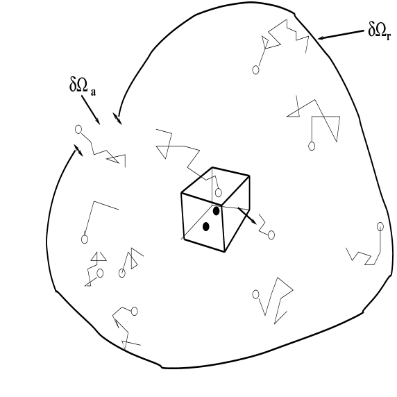
Figure 1: Chemical reaction inside a microdomain. Each free particle (white circle) moves according to a Brownian motion until it binds to a free site (black color). An occupied site cannot accept any other particles. A molecule is composed of a finite number of sites. Parts of the microdomain is reflective and the rest is absorbing.

which represents diffusion with coefficient $D$. Additional change in the contents of the volume $\Delta\mbox{\boldmath$x$}$ is due to the binding and unbinding of $M$ particles to the substrate. When there are $S$ free binding sites in the volume $\Delta\mbox{\boldmath$x$}$ (see Figure 1), the probability that one $M$ particle binds to a free site in the volume $\Delta\mbox{\boldmath$x$}$ in the time interval $[t,t+\Delta t]$ is proportional both to $S$ and to the number $M_{\mbox{free}}(\mbox{\boldmath$x$},t)$ of free $M$ particles in the volume $\Delta\mbox{\boldmath$x$}$ . It is given by

$$k_{1}M_{0}p(\mbox{\boldmath$x$},S,t)S\Delta\mbox{\boldmath$x$}\,\Delta t.$$

The probability that one particle unbinds in the volume $\Delta\mbox{\boldmath$x$}$ in this time interval is proportional to the number $s_{0}(\mbox{\boldmath$x$})\Delta\mbox{\boldmath$x$}-S$ of bound sites in the volume $\Delta\mbox{\boldmath$x$}$ , given by

$$k_{-1}[s_{0}\Delta\mbox{\boldmath$x$}-S]\Delta t.$$

Thus the probability of $S$ free sites when no change occurred in the number of free sites is

$$p(\mbox{\boldmath$x$},S,t)\Delta\mbox{\boldmath$x$}\left\{1-k_{1}M_{0}p(\mbox{\boldmath$x$},S,t)S\,\Delta\mbox{\boldmath$x$}\,\Delta t-k_{-1}[s_{0}(\mbox{\boldmath$x$})\Delta\mbox{\boldmath$x$}-S]\Delta t\right\}.$$

The number of free sites can change to $S$ at the end of the interval $[t,t+\Delta t]$ if it was $S+1$ at the beginning and one bond was formed, or if it was $S-1$ and one particle was unbound. The probability of this event, as calculated above, is

$$k_{1}M_{0}\,\Delta\mbox{\boldmath$x$}\,(S+1)p(\mbox{\boldmath$x$},S+1,t)\,\Delta t+k_{-1}[s_{0}(\mbox{\boldmath$x$})\Delta\mbox{\boldmath$x$}-S+1)]\Delta t.$$

The probability of $\mbox{\boldmath$x$},S$ at time $t+\Delta t$ is therefore

$$p(\mbox{\boldmath$x$},S,t+\Delta t)\Delta\mbox{\boldmath$x$}=$$

$$-\nabla\cdot\mbox{\boldmath$J$}(\mbox{\boldmath$x$},S,t\,|\,\mbox{\boldmath$y$})\,\Delta\mbox{\boldmath$x$}+$$

$$p(\mbox{\boldmath$x$},S,t)\Delta\mbox{\boldmath$x$}\{1-M_{0}k_{1}\Delta\mbox{\boldmath$x$}\,Sp(\mbox{\boldmath$x$},S,t)\Delta t-k_{-1}[s_{0}(\mbox{\boldmath$x$})\Delta\mbox{\boldmath$x$}-S]\Delta t\}+$$

$$M_{0}k_{1}(S+1)p^{2}(\mbox{\boldmath$x$},S+1,t)\,(\Delta\mbox{\boldmath$x$})^{2}\Delta t+$$

$$k_{-1}[s_{0}(\mbox{\boldmath$x$})\Delta\mbox{\boldmath$x$}-S+1]p(\mbox{\boldmath$x$},S-1,t)\Delta\mbox{\boldmath$x$}\Delta t.$$

for $S=0,1,2,\dots,S_{\mbox{max}}$, the coupled partial differential equations

$$\frac{\partial p(\mbox{\boldmath$x$},S,t)}{\partial t} = -\nabla\cdot\mbox{\boldmath$J$}(\mbox{\boldmath$x$},S,t)-K_{1}p^{2}(\mbox{\boldmath$x$},S,t)S-k_{-1}[S_{0}(\mbox{\boldmath$x$})-S]p(\mbox{\boldmath$x$},S,t)$$

$$+ K_{1}(S+1)p^{2}(\mbox{\boldmath$x$},S+1,t)+k_{-1}[S_{0}(\mbox{\boldmath$x$})-S+1]p(\mbox{\boldmath$x$},S-1,t),$$

where by definition $\mbox{\boldmath$J$}(\mbox{\boldmath$x$},S,t)$ is the joint probability flux at position $x$ at time $t$, and $S$ proteins are free. It is defined in the diffusion case by

$$\mbox{\boldmath$J$}(\mbox{\boldmath$x$},S,t)=-D\nabla p(\mbox{\boldmath$x$},S,t).$$ (7)

The new (forward) binding rate is

$$K_{1}=M_{0}k_{1}\Delta\mbox{\boldmath$x$}$$

and

$$S_{0}(\mbox{\boldmath$x$})=s_{0}(\mbox{\boldmath$x$})\,\Delta\mbox{\boldmath$x$}=\mbox{total number of binding sites in the volume $\Delta\mbox{\boldmath$x$}$ }.$$

Thus $K_{1}$ is the probability flux into the binding sites. The boundary conditions on $S$ are

$$p(\mbox{\boldmath$x$},S,t)=0\quad\mbox{for $S<0$ and $S>S_{0}(\mbox{\boldmath$x$})$}.$$ (8)

Remark 1. By summing equation (LABEL:eqff) over $0\leq S\leq S_{0}(\mbox{\boldmath$x$})$ and using the boundary conditions (8), we obtain

$$\frac{\partial M_{\mbox{total}}(\mbox{\boldmath$x$},t)}{\partial t}=-\nabla\cdot\mbox{\boldmath$J$}_{M}(\mbox{\boldmath$x$},t),$$ (9)

for the marginal density of the $M$ particles. It means that all bound and free $M$ particles effectively diffuse.

Remark 2. When at specific locations there can be at most one binding site, the system (LABEL:eqff) reduces to the coupled equations

$$\frac{\partial p(\mbox{\boldmath$x$},0,t)}{\partial t}=D\Delta p(\mbox{\boldmath$x$},0,t)-k_{-1}p(\mbox{\boldmath$x$},0,t)+K_{1}p^{2}(\mbox{\boldmath$x$},1,t)$$

(10)

$$\frac{\partial p(\mbox{\boldmath$x$},1,t)}{\partial t}=D\Delta p(\mbox{\boldmath$x$},1,t)+k_{-1}p(\mbox{\boldmath$x$},0,t)-K_{1}p^{2}(\mbox{\boldmath$x$},1,t).$$

Here $S_{0}(\mbox{\boldmath$x$})$ can take the values 0 or 1. When no molecules can escape from a bounded domain, the flux associated with $p(\mbox{\boldmath$x$},S,t)$ satisfies the reflective boundary condition

$$\left.\mbox{\boldmath$J$}\cdot\mbox{\boldmath$n$}\right|_{\partial\Omega}=0.$$ (11)

The initial condition, when no substrate is bound, is given by $p(\mbox{\boldmath$x$},0,0)=m_{0}(\mbox{\boldmath$x$})$, hence $p(\mbox{\boldmath$x$},1,0)=0$. When the total number of $M$ particles stays constant (i.e., no particles leave the domain), adding equations (2.1) gives in the steady state

$$p(\mbox{\boldmath$x$},0)+p(\mbox{\boldmath$x$},1)=\frac{1}{|\Omega|}.$$ (12)

If the $M$ particles can escape the compartment, e.g., by being absorbed in a part of the boundary $\partial\Omega_{a}$, the condition (11) should be changed to

$$\left.\mbox{\boldmath$J$}\cdot\mbox{\boldmath$n$}\right|_{\partial\Omega-\partial\Omega_{a}}=0$$ (13)

and

$$\left.p(\mbox{\boldmath$x$},S,t)\right|_{\partial\Omega_{a}}=0.$$ (14)

In this case (12) no longer holds.

Remark 3: Obviously, $S_{0}(\mbox{\boldmath$x$})$ takes only integer values. We assume that its discontinuities are located on smooth interfaces. The density $p(\mbox{\boldmath$x$},S,t)$ and the normal component of the flux $\mbox{\boldmath$J$}(\mbox{\boldmath$x$},S,t)\cdot\mbox{\boldmath$n$}(\mbox{\boldmath$x$})$ are continuous across the interfaces for all $S=0,1,\dots,S_{\mbox{max}}$.

2.2 Moments of the pdf

Statistical moments of the pdf can be computed from equation (LABEL:eqff). The average and the standard deviation of the number of bound proteins are evaluated for equation (2.1). The mean of the number of bound proteins at time $t$ is given by

$$\langle S_{b}(t)\rangle=\int_{\Omega}S_{0}(\mbox{\boldmath$x$})p(\mbox{\boldmath$x$},1,t)d\mbox{\boldmath$x$}.$$ (15)

The standard deviation is given by

$$\sigma^{2}(t)=\langle S_{b}^{2}(t)\rangle-\langle S_{b}(t)\rangle^{2}=\int_{\Omega}S^{2}_{0}(\mbox{\boldmath$x$})p(\mbox{\boldmath$x$},1,t)\,d\mbox{\boldmath$x$}-\left(\int_{\Omega}S_{0}(\mbox{\boldmath$x$})p(\mbox{\boldmath$x$},1,t)\,d\mbox{\boldmath$x$}\right)^{2}.$$ (16)

When the proteins are uniformly distributed on a subset $\Omega^{\prime}\subset\Omega$, the distribution $S_{0}(\mbox{\boldmath$x$})$ is given by the characteristic function of the subset $\Omega^{\prime}$,

$$S_{0}(\mbox{\boldmath$x$})=\chi_{\Omega^{\prime}}(\mbox{\boldmath$x$})\frac{N_{0}}{\mid\Omega^{\prime}\mid},$$ (17)

where the total number of binding sites is

$$N_{0}=\int_{\Omega}S_{0}(\mbox{\boldmath$x$})\,d\mbox{\boldmath$x$}.$$

We obtain the standard deviation of bound sites from the expression (16) as

$$\sigma^{2}(t) = \langle S_{b}^{2}(t)\rangle-\langle S_{b}(t)\rangle^{2}$$

$$= \left(\frac{N_{0}}{\mid\Omega^{\prime}\mid}\right)^{2}\left(\bar{S_{0}}(t)-\bar{S_{0}}^{2}(t)\right)=\left(\frac{N_{0}}{\mid\Omega^{\prime}\mid}\right)^{2}\bar{S_{0}}(t)(1-\bar{S_{0}}(t)),$$

where

$$\bar{S_{0}}(t)=\int_{\Omega^{\prime}}p(\mbox{\boldmath$x$},1,t)\,d\mbox{\boldmath$x$}$$ (19)

is the fraction of bound sites. Note that

$$\bar{S_{0}}(t)\leq 1.$$

2.3 Standard deviation of the number of bound protein in some cases

We consider the one-dimensional case where $\Omega=[0,L]$ and $S_{0}(x)$ is either 0 or 1 in intervals. In the steady state the system (2.1) is

$$0 = D\Delta p(x,0)-k_{-1}S_{0}(x)p(x,0)+K_{1}p^{2}(x,1)$$

$$0 = D\Delta p(x,1)+k_{-1}S_{0}(x)p(x,0)-K_{1}p^{2}(x,1)$$ (20)

$$\frac{1}{L} = p(x,0)+p(x,1),$$

which reduces to

$$Dp^{\prime\prime}(x,1)+k_{-1}S_{0}(x)\left[\frac{1}{L}-p(x,1)\right]-K_{1}p^{2}(x,1)=0.$$ (21)

We convert to densities by setting

$$c_{M}(x,1)=M_{0}p(x,1).$$

Then (21) becomes

$$Dc_{M}^{\prime\prime}(x,1)+k_{-1}S_{0}(x)\left[\frac{M_{0}}{L}-c_{M}(x,1)\right]-\frac{K_{1}}{M_{0}}c_{M}^{2}(x,1)=0.$$ (22)

The function $c_{M}(x,1)$ is supported where the protein are located.

When the boundary conditions are reflective for the $M$ trajectories, using the uniqueness of the solution, then at a point $x$, where $S_{0}(x)$ is supported is

$$c_{M}(x,1)=\frac{2k_{-1}S_{0}(x)M_{0}/L}{k_{-1}S_{0}(x)+\sqrt{(k_{-1}S_{0}(x))^{2}+4K_{1}k_{-1}S_{0}(x)/L}}.$$

In particular, If the substrate is uniformly distributed in intervals $S_{0}(x)=N_{S}/L$ and $M_{0}\ll N_{S}$, then the fraction of bound $M$ particles is

$$p_{M}=\frac{1}{M_{0}}\int_{0}^{L}c_{M}(x,1)\,dx=\frac{2}{1+\sqrt{1+4\displaystyle\frac{M_{0}k_{1}\Delta x}{N_{S}k_{-1}}}}\sim 1,$$ (23)

which means that practically all $M$ particles are bound. If $M_{0}\gg N_{S}$, then (23) gives

$$p_{M}=\frac{1}{M_{0}}\int_{0}^{L}c_{M}(x,1)\,dx\sim\sqrt{\frac{N_{S}k_{-1}}{M_{0}k_{1}\,\Delta x}}\ll 1.$$ (24)

In this case, the variance of the fluctuations in the number of bound $M$ particles, which is the same as the number of bound sites, as a function of $M_{0}$ and $N_{S}$, is given by

$$\sigma^{2}_{S}(M_{0})=p_{M}(1-p_{M})=\frac{2}{1+\sqrt{1+4\displaystyle\frac{M_{0}k_{1}\Delta x}{N_{S}k_{-1}}}}\left(1-\frac{2}{1+\sqrt{1+4\displaystyle\frac{M_{0}k_{1}\Delta x}{N_{S}k_{-1}}}}\right).$$ (25)

The graph of $\sigma^{2}_{S}(M_{0})$ vanishes for both $M_{0}\to 0$ and $M_{0}\to\infty$ and has a unique finite maximum, as in figure 4

2.4 General equations when binding proteins are located on the boundary of the domain

We consider the same problem, but with binding sites located on the boundary $\partial\Omega$ with surface density $S_{0}(\mbox{\boldmath$x$})$ (see figure 2). This may represent for example binding to gated channels, which open when they bind agonist molecules. Some channels may need to bind several agonist molecules to open, however, we consider here the case that a single agonist molecules opens the channel upon binding. We assume that the agonist molecule cannot escape $\Omega$.

The initial $M_{0}$ agonist molecules diffuse in $\Omega$ and are reflected at $\partial\Omega$ at non binding sites, but can bind to a free binding site on a protein channel in the membrane with a certain forward binding rate $k_{1}$. When this occurs the channel opens and stays open as long as the agonist is bound. The bound agonist is released from the bound state at a backward rate $k_{-1}$. Then the number of open channels is the number of missing $M$ particles in $\Omega$. We write

$$M_{0}=\int_{\Omega}c(\mbox{\boldmath$x$},t)\,d\mbox{\boldmath$x$}+\int_{\partial\Omega}S_{\mbox{bound}}(\mbox{\boldmath$x$},t)\,dS_{\mbox{\boldmath$x$}.}$$

The equations for the density of $M$ particles in $\Omega$ and in $\partial\Omega$ is

$$\frac{\partial c(\mbox{\boldmath$x$},t)}{\partial t} = D\Delta c(\mbox{\boldmath$x$},t)$$

$$-D\frac{\partial c(\mbox{\boldmath$x$},t)}{\partial\mbox{\boldmath$n$}} = \mbox{\boldmath$J$}(\mbox{\boldmath$x$},t)\cdot\mbox{\boldmath$n$}(\mbox{\boldmath$x$}){\Bigg{|}}_{\mbox{\boldmath$x$}\in\partial\Omega}=\dot{S}_{\mbox{bound}}(\mbox{\boldmath$x$},t)$$ (26)

$$= k_{1}c(\mbox{\boldmath$x$},t)[S_{0}(\mbox{\boldmath$x$})-S_{\mbox{bound}}(\mbox{\boldmath$x$},t)]-k_{-1}S_{\mbox{bound}}(\mbox{\boldmath$x$},t).$$

The probability of $k$ bound sites on the boundary at time $t$ satisfies the equations

$$\dot{P}_{k}(t) = -P_{k}(t)K_{1}\oint_{\partial\Omega}c(\mbox{\boldmath$x$},t)\left[S_{0}(\mbox{\boldmath$x$})-S_{\mbox{bound}}(\mbox{\boldmath$x$},t)\right]\,dS_{\mbox{\boldmath$x$}}-kP_{k}(t)k_{-1}$$ (27)

$$+P_{k-1}(t)K_{1}\oint_{\partial\Omega}c(\mbox{\boldmath$x$},t)\left[S_{0}(\mbox{\boldmath$x$})-S_{\mbox{bound}}(\mbox{\boldmath$x$},t)\right]\,dS_{\mbox{\boldmath$x$}}+(k+1)P_{k+1}(t)k_{-1},,$$

$$\dot{P}_{0}(t) = -P_{0}(t)K_{1}\oint_{\partial\Omega}c(\mbox{\boldmath$x$},t)\left[S_{0}(\mbox{\boldmath$x$})-S_{\mbox{bound}}(\mbox{\boldmath$x$},t)\right]\,dS_{\mbox{\boldmath$x$}}+P_{1}(t)k_{-1},,$$ (28)

$$\dot{P}_{S_{0}}(t) = -P_{S_{0}}(t)K_{1}\oint_{\partial\Omega}c(\mbox{\boldmath$x$},t)\left[S_{0}(\mbox{\boldmath$x$})-S_{\mbox{bound}}(\mbox{\boldmath$x$},t)\right]\,dS_{\mbox{\boldmath$x$}}-S_{0}P_{S_{0}}(t)k_{-1}$$ (29)

$$+P_{S_{0}-1}(t)K_{1}\oint_{\partial\Omega}c(\mbox{\boldmath$x$},t)\left[S_{0}(\mbox{\boldmath$x$})-S_{\mbox{bound}}(\mbox{\boldmath$x$},t)\right]\,dS_{\mbox{\boldmath$x$}}$$

where, according to eq.(26)

$$\dot{S}_{\mbox{bound}}(\mbox{\boldmath$x$},t)=k_{1}c(\mbox{\boldmath$x$},t)[S_{0}(\mbox{\boldmath$x$})-S_{\mbox{bound}}(\mbox{\boldmath$x$},t)]-k_{-1}S_{\mbox{bound}}(\mbox{\boldmath$x$},t).$$

Here $0\leq k\leq S_{0}$, where

$$S_{0}=\oint_{\partial\Omega}S_{0}(\mbox{\boldmath$x$})\,dS_{\mbox{\boldmath$x$}},$$

that is, $P_{-1}(t)=P_{S_{0}+1}(t)=0$.

The moments of the number of bound sites are

$$\langle S_{b}(t)\rangle=\sum_{k=1}^{S_{0}}kP_{k}(t),\quad\langle S_{b}^{2}(t)\rangle=\sum_{k=1}^{S_{0}}k^{2}P_{k}(t).$$

The variance in the number of bound sites is

$$\sigma^{2}(t)=\langle S_{b}^{2}(t)\rangle-\langle S_{b}(t)\rangle^{2}.$$

3 The fluctuation in the number of particles in a push-pull chemical reaction

A push-pull chemical reaction consists of a source that produces particles at a given rate and a sink or a killing term that destroy or remove the particles from the system with its rate. When the movement of the particles is driven by diffusion and the source and the sink are not uniformly distributed, the number of particles fluctuates. In this section, we propose an approach to estimate the mean number and the fluctuations. A permanent regime imposes that the rate of the sink and the source satisfy some specific conditions. At equilibrium, in the limit of a large number particles, the push-pull mechanism reaches a steady state and the number of particles does not fluctuate and can be computed using the rate constant. But for a small number, the analysis requires to study separately the dynamics of the particles and especially the law of injection by the source.

In the neurobiological context, many biochemical reactions are based on push-pull mechanisms: at a given location, a source produces molecules and somewhere else, an enzyme modeled as a sink, destroys the molecules with a certain efficassy. In general, sinks and sources are not uniformly distributed, which induces fluctuations. As an example, gating molecules that can open channels are produced by such push-pull mechanism, and the fluctuations in the number of molecules induce a fluctuation in the number of open channels, which is reveals at the cellular level. It is of particular interest to examine the situation where molecules move by diffusion, the enzyme sink is represented by a single molecule and the sources are uniformly distributed. For example, this occurs inside a compartment of photo-receptors for the regulation of cGMP molecules.

3.1 The push-pull mechanism

The sink of the push-pull mechanism is modelled by a killing term located at a single point. The killing term is a Dirac function, ( see [11] for the exact mathematical interpretation). The source is assumed to be uniformly distributed and molecules are produced at a constant rate $\gamma$.

We assume that the molecules are independent and their movement in a domain $\Omega$ can be described by the stochastic differential equations

$$\dot{\mbox{\boldmath$x$}}_{k}=\mbox{\boldmath$b$}(\mbox{\boldmath$x$}_{k})+\sqrt{2D}\,\dot{\mbox{\boldmath$w$}}_{k},\quad k=1,\ldots,N,$$ (30)

where $\mbox{\boldmath$b$}(\mbox{\boldmath$x$})$ is a drift vector. Since the molecules cannot escape, reflecting boundary conditions are imposed at the boundary $\partial\Omega$. If a particle is injected in $\Omega$ at time $t=0$, its pdf $p(\mbox{\boldmath$x$},t)$ satisfies the Fokker-Planck equation

$$\frac{\partial p(\mbox{\boldmath$x$},t)}{\partial t} = -\nabla\cdot{\mbox{\boldmath$J$}}(\mbox{\boldmath$x$},t)-k_{1}\delta(\mbox{\boldmath$x$}-\mbox{\boldmath$x$}_{1})p(\mbox{\boldmath$x$},t)$$

$$\left.\mbox{\boldmath$J$}\cdot\mbox{\boldmath$n$}\right|_{\partial\Omega} = 0,$$

where the probability flux density vector is given by

$$\mbox{\boldmath$J$}(\mbox{\boldmath$x$},t)=-D\nabla p(\mbox{\boldmath$x$},t)+\mbox{\boldmath$b$}(\mbox{\boldmath$x$})p(\mbox{\boldmath$x$},t).$$ (32)

At any moment of time, when there are $N$ particles inside $\Omega$, the concentration $c(\mbox{\boldmath$x$},t)$ is given by

$$c(\mbox{\boldmath$x$},t)=Np(\mbox{\boldmath$x$},t).$$ (33)

Particles are injected with a Poisson stream at a rate $\gamma$, that is, at independent and identically distributed inter-injection times, whose pdf is

$$f(t)=\gamma e^{-\gamma t}.$$

The mean inter-injection time is $E(T)=\gamma^{-1}$. The probability that a molecule injected at time $t=0$ at a point $y$ survives at time $t$ is

$$S_{\mbox{\boldmath$y$}}(t)=Pr\{\mbox{\boldmath$x$}(t)\in\Omega\}=\int_{\Omega}p(\mbox{\boldmath$x$},t\,|\,\mbox{\boldmath$y$})\,d\mbox{\boldmath$x$}.$$ (34)

When $\mbox{\boldmath$y$}=\mbox{\boldmath$0$}$, we denote $S(t)=S_{\mbox{\boldmath$0$}}(t)$. To compute the mean and the variance of the number of molecules $N(t)$ surviving in $\Omega$ at time $t$, we use here the renewal equation [4, 3, 20],

$$\Pr\{N(t)=0\} = \Pr\{\mbox{\boldmath$x$}(t)\notin\Omega\}\cdot\left[\int_{0}^{t}f(s)\Pr\{N(t-s)=0\}\,ds+\int_{t}^{\infty}f(s)\,ds\right]$$ (35)

$$\Pr\{N(t)=1\} = \Pr\{\mbox{\boldmath$x$}(t)\in\Omega\}\cdot\left[\int_{0}^{t}f(s)\Pr\{N(t-s)=0\}\,ds+\int_{t}^{\infty}f(s)\,ds\right]$$ (36)

$$+\Pr\{\mbox{\boldmath$x$}(t)\notin\Omega\}\cdot\int_{0}^{t}f(s)\Pr\{N(t-s)=1\}\,ds.$$

$$\Pr\{N(t)=n\} = \Pr\{\mbox{\boldmath$x$}(t)\in\Omega\}\cdot\int_{0}^{t}f(s)\Pr\{N(t-s)=n-1\}\,ds$$ (37)

$$+\Pr\{\mbox{\boldmath$x$}(t)\notin\Omega\}\cdot\int_{0}^{t}f(s)\Pr\{N(t-s)=n\}\,ds,\quad n>1.$$

The expected number $EN(t)$ of molecules surviving in $\Omega$ at time $t$ is

$$EN(t) = \sum_{n=1}^{\infty}n\Pr\{N(t)=n\}$$ (38)

$$= \Pr\{\mbox{\boldmath$x$}(t)\in\Omega\}\cdot\left(\int_{0}^{t}f_{L}(s)EN(t-s)\,ds+\int_{0}^{\infty}f(s)\,ds\right)$$

$$+\Pr\{\mbox{\boldmath$x$}(t)\notin\Omega\}\cdot\int_{0}^{t}f(s)EN(t-s)\,ds$$

$$= \Pr\{\mbox{\boldmath$x$}(t)\in\Omega\}+\int_{0}^{t}f(s)EN(t-s)\,ds.$$

The integral equation (38) is solved by the Laplace transform as

$$\bar{n}(\tau)=\frac{\bar{S}(\tau)}{1-\bar{f}(\tau)},$$ (39)

where $\bar{S}(\tau)$ is the Laplace transform of $\Pr\{\mbox{\boldmath$x$}(t)\in\Omega\}$ when the initial position of insertion is 0.

$$\bar{f}(\tau)=\frac{\gamma}{\gamma+\tau}$$ (40)

and $\bar{S}(\tau)$ is the Laplace transform of the survival probability. Therefore the Laplace transform of $EN(t)$ is given by

$$\bar{n}(\tau)=\frac{(\gamma+\tau)\bar{S}(\tau)}{\tau}.$$ (41)

3.1.1 Computation of $\bar{S}(\tau)$ in a driftless one-dimensional model

We consider the one-dimensional equation (3.1) in $\Omega=[0,L]$ and $\mbox{\boldmath$b$}(\mbox{\boldmath$x$})=\mbox{\boldmath$0$}$. We assume, for simplicity, that $L=\pi$ and $D=1$.

The survival probability given by $S(t)=\displaystyle\int_{0}^{L}p(x,t\,|\,y)dx$ is also (see [11]) equal to

$$S(t)=1-k_{1}\int^{t}_{0}p(x,t\,|\,y)dx.$$ (42)

The Laplace transform is

$$\bar{S}(\tau)=\frac{1-k_{1}\bar{p}(x_{1},\tau\,|\,y)}{\tau}.$$ (43)

$\bar{p}(x_{1},\tau\,|\,y)$ can be computed using the Green’s function for the Neumann problem for (3.1), given by

$$G(x,t\,|\,y)=1+\frac{2}{\pi}\sum_{n=1}^{\infty}e^{-n^{2}t}\cos nx\cos ny.$$ (44)

Following the computations of [11], an integral representation of the solution of equation 3.1 is given by

$$p(x,t\,|\,y)=-k_{1}\int_{0}^{t}p(x_{1},s\,|\,y)G(x,t-s\,|\,x_{1})\,ds+\,G(x,t\,|\,y).$$ (45)

The Laplace transform of equation (45) is given by

$$\bar{p}(x,\tau\,|\,y)=-k_{1}\bar{p}(x_{1},\tau\,|\,y)\bar{G}(x,\tau\,|\,x_{1})\,ds+\,\bar{G}(x,\tau\,|\,y).$$ (46)

Thus,

$$\bar{p}(x_{1},\tau\,|\,y)=\frac{\bar{G}(x_{1},\tau\,|\,y)}{1+k_{1}\bar{G}(x_{1},\tau\,|\,x_{1})}$$ (47)

and

$$\bar{p}(x,\tau\,|\,y)=\frac{1}{k_{1}}+\frac{\bar{G}(x_{1},\tau\,|\,y)-\bar{G}(x_{1},\tau\,|\,x_{1})-k^{-1}_{1}}{1+k_{1}\bar{G}(x_{1},\tau\,|\,x_{1})}.$$ (48)

With

$$\bar{G}(x,\tau\,|\,y)=\frac{1}{\tau}+\frac{2}{\pi}\sum_{n=1}^{\infty}\frac{\cos nx\cos ny}{n^{2}+\tau},$$ (49)

for $x,y\in(0,\pi)$, and to first order in $\tau$, we obtain

$$\bar{p}(x,\tau\,|\,y) = \frac{1}{k_{1}}+\frac{\displaystyle\frac{2}{\pi}\sum_{n=1}^{\infty}\left[\displaystyle\frac{\cos nx\cos ny}{n^{2}}-\displaystyle\frac{\cos^{2}nx}{n^{2}}\right]-k^{-1}_{1}}{k_{1}+\displaystyle\frac{2k_{1}}{\pi}\sum_{n=1}^{\infty}\displaystyle\frac{\cos nx\cos ny}{n^{2}}}\tau+o(\tau)$$

$$= \frac{1}{k_{1}}+\frac{\displaystyle\frac{1}{2\pi}(x^{2}-y^{2})-k^{-1}_{1}}{k_{1}\left(1+\displaystyle\frac{2}{\pi}\left(\displaystyle\frac{\pi^{2}}{6}-\displaystyle\frac{\pi}{2}x+\frac{x^{2}}{2}\right)\right)}\tau+o(\tau).$$

Hence

$$\bar{S}(\tau) = \frac{1-k_{1}\bar{p}(x_{1},\tau\,|\,y)}{\tau}$$

$$= \frac{\displaystyle\frac{-1}{2\pi}\left(x^{2}-y^{2}\right)+k^{-1}_{1}}{\left(1+\displaystyle\frac{2}{\pi}\left(\displaystyle\frac{\pi^{2}}{6}-\displaystyle\frac{\pi}{2}x+\displaystyle\frac{x^{2}}{2}\right)\right)}+o(1).$$

Using the normalization condition that $S(0)=1$, we find the long time asymptotics

$$S(t)\sim_{r\rightarrow+\infty}\exp(-\alpha t),$$ (50)

where

$$\alpha^{-1}=\frac{\displaystyle\frac{-1}{2\pi}\left(x^{2}-y^{2}\right)+k^{-1}_{1}}{\left(1+\displaystyle\frac{2}{\pi}\left(\displaystyle\frac{\pi^{2}}{6}-\displaystyle\frac{\pi}{2}x+\displaystyle\frac{x^{2}}{2}\right)\right)}.$$ (51)

The un-normalized time constant for $x,y\in[0,L]$ is

$$\alpha^{-1}=\frac{\displaystyle\frac{-\pi^{3}}{2D}\left(x^{2}-y^{2}\right)+k^{-1}_{1}}{\left(1+\displaystyle 2\pi\left(\displaystyle\frac{1}{6}-\displaystyle\frac{1}{2L}x+\displaystyle\frac{x^{2}}{L^{2}}\right)\right)}.$$ (52)

3.1.2 The steady state limit

In the steady state, the mean number of molecules $N(t)$ surviving in $\Omega$ at time $t$ is

$$\lim_{t\rightarrow\infty}EN(t)=\lim_{\tau\rightarrow 0}\tau\bar{n}(\tau)=\gamma\bar{S}(0)$$ (53)

Note that

$$\bar{S}(0)=\int_{0}^{\infty}\int_{0}^{L}p(x,t|0)\,dx.$$

If at time $t=0$ the particle is injected randomly at a point $y$, we index $S$ by $y$ and write

$$\bar{S_{y}}(0)=\int_{0}^{\infty}\int_{0}^{L}p(x,t|y)dx=\int_{0}^{L}G(x|y)dy$$

where $G(x\,|\,y)$ is the solution of

$$-\delta(x-y) = D\frac{\partial^{2}G}{\partial x^{2}}-k\delta(x-x_{1})G$$

$$\frac{\partial G(0\,|\,y)}{\partial x} = \frac{\partial G(L\,|\,y)}{\partial x}=0.$$

Thus,

$$G(x\,|\,y)=-\frac{\theta(x-y)}{D}+\frac{\theta(x-x_{1})}{D}+\frac{1}{k_{1}},$$

where $\theta(x)$ is the integral of the Heaviside unit step function. It follows that

$$\bar{S}_{y}(0)=\int_{0}^{L}G(x\,|\,y)dy=-\frac{(L-y)^{2}}{2D}+\frac{(L-x_{1})^{2}}{2D}+\frac{L}{k_{1}}.$$

At steady state, the mean number of molecules surviving in $\Omega$ at time $t$ is given by

$$N_{y}(\infty)=\gamma\bar{S}_{y}(0)=\gamma(-\frac{(L-y)^{2}}{2D}+\frac{(L-x_{1})^{2}}{2D}+\frac{L}{k_{1}})$$ (54)

If the particle is initially uniformly distributed, $\Pr\{y\in[x,x+dx]\}=\displaystyle\frac{dx}{L}$, then the steady state mean number of surviving molecules is given by

$$N(\infty)=\gamma E_{y}[\bar{S_{y}}(0)]=\gamma\left(-\frac{L^{2}}{6D}+\frac{(L-x_{1})^{2}}{2D}+\frac{L}{k_{1}}\right).$$ (55)

3.1.3 Variance

The second moment of the total number of surviving particles is defined as

$$EN^{2}(t)=\sum_{n=1}^{\infty}n^{2}\Pr\{N(t)=n\}.$$

We will now compute such number using the renewal equations. We have

$$EN^{2}(t) = \Pr\{x(t)\in\Omega\}\int_{0}^{t}f(s)k^{2}\Pr\{N(t-s)=k-1\}\,ds$$

$$+\Pr\{x(t)\notin[0,L]\}\int_{0}^{t}f(s)k^{2}\Pr\{N(t-s)=k\}\,ds+\Pr\{x(t)\notin\Omega\}\int_{t}^{\infty}f(s)\,ds,$$

which leads to

$$EN^{2}(t) = \Pr\{x(t)\in[0,L]\}\int_{t}^{\infty}f(s)\,ds+\Pr\{x(t)\in\Omega\}\int_{0}^{t}EN^{2}(t-s)f(s)\,ds+$$

$$\Pr\{x(t)\notin[0,L]\}\int_{0}^{t}EN^{2}(t-s)f(s)\,ds$$

$$+ \sum_{k}\Pr\{x(t)\in\Omega\}\int_{0}^{t}(2k+1)Pr\{N(t)=k-1\}f(s)\,ds.$$

Thus,

$$EN^{2}(t) = \int_{0}^{t}EN^{2}(t-s)f(s)\,ds+\Pr\{x(t)\in\Omega\}\int_{t}^{\infty}f(s)\,ds+$$

$$2\Pr\{x(t)\in\Omega\}\int_{0}^{t}E(N(t-s)f(s)\,ds+\Pr\{x(t)\in\Omega\}\int_{0}^{t}f(s)\,ds$$

and

$$EN^{2}(t)=\int_{0}^{t}EN^{2}(t-s)f(s)\,ds+\Pr\{x(t)\in\Omega\}+2\Pr\{x(t)\in\Omega\}\int_{0}^{t}f(s)E(N(t-s))ds.$$ (56)

Remark.

The variance can also be written in the form

$$\sigma^{2}_{N}(t)=EN^{2}(t)-[E(N(t))]^{2}=\Pr\{x(t)\in\Omega\}-\Pr\{x(t)\in\Omega\}^{2}+$$

$$\int_{0}^{t}EN^{2}(t-s)f(s)\,ds-\left(\int_{0}^{t}E(N(t-s))f(s)\,ds\right)^{2}.$$

3.1.4 The steady state variance

To compute the variance in the steady state limit, as $t\rightarrow\infty$, we Laplace transform equation (56),

$$\bar{n^{2}}(\tau)=\frac{\bar{S}(\tau)}{1-\bar{f}(\tau)}+\frac{2}{1-\bar{f}(\tau)}\int^{\infty}_{0}\left[S(t)\int_{0}^{t}f(t-s)n(s)\,ds\right]e^{-t\tau}\,dt.$$

It follows that

$$EN^{2}(\infty)=\lim_{t\rightarrow\infty}EN^{2}(t)=\lim_{\tau\rightarrow 0}\tau\bar{n^{2}}(\tau).$$

Writing

$$\tau\bar{n^{2}}(\tau)=I(\tau)+II(\tau),$$

we obtain the short $\tau$ approximation

$$I(\tau)=\tau\frac{\bar{S}(\tau)}{1-\bar{f}(\tau)}\sim\gamma\bar{S}(0).$$

To evaluate

$$II(\tau)=\tau\frac{2}{1-\bar{f}(\tau)}\int^{\infty}_{0}\left[S(t)\int_{0}^{t}f(t-s)n(s)\,ds\right]e^{-t\tau}\,dt,$$

we recall that $f(t)=\gamma e^{-\gamma t}$ and approximating $S(t)$ by $e^{-\alpha t}$ and interchanging the order of integration, we obtain

$$II(\tau) = \tau\gamma\frac{2}{1-\bar{f}(\tau)}\int^{\infty}_{0}n(s)e^{\gamma s}\int_{s}^{\infty}e^{-t(\gamma+\tau+\alpha)}dt,$$

$$= \tau\gamma\frac{2}{1-\bar{f}(\tau)}\frac{1}{\gamma+\tau+\alpha}\int^{\infty}_{0}n(s)e^{-t(\tau+\alpha)}dt,$$

$$= \tau\gamma\frac{2}{1-\bar{f}(\tau)}\frac{1}{\gamma+\tau+\alpha}\bar{n}(\tau+\alpha)$$

$$\sim 2\gamma^{2}\frac{1}{\gamma+\alpha}\bar{n}(\alpha).$$

Finally,

$$EN^{2}(\infty)=\gamma\bar{S}(0)+2\gamma^{2}\frac{1}{\gamma+\alpha}\bar{n}(\alpha)$$

and

$$\sigma^{2}=EN^{2}(\infty)-\left(EN(\infty)\right)^{2}=\gamma\bar{S}(0)-\gamma^{2}\bar{S}^{2}(0)+\frac{2\gamma^{2}}{\gamma+\alpha}\bar{n}(\alpha),$$ (57)

where $\bar{S}(0)=\displaystyle\frac{N(\infty)}{\gamma}$, the time $\alpha$ depends only on $k_{1}$, the diffusion constant and the length $L$, as given in formula (52), and $\bar{n}(\alpha)=\displaystyle\frac{\gamma+\alpha}{\alpha}\bar{S}(\alpha)$, where $\bar{S}(\alpha)$ is the Laplace transform of the survival probability at time $\alpha$.

3.2 Push-pull chemical reaction in the continuum limit

When the number of reacting molecules is large enough, regulated by a push-pull mechanism of hydrolysis and synthesis, the reaction-diffusion equations is sufficient to describe the evolution of such system. We assume that the molecules diffuse inside a domain $\Omega$, but the synthesis occurs only uniformly in a domain $\Omega^{\prime}\subset\Omega$ while the hydrolysis is performed by isolated enzymes. The hydrolysis can be modelled as a killing measure $k(\mbox{\boldmath$x$})$ (see [11]). When there are a discreet number $N_{h}$ of killing sources, the killing measure $k(\mbox{\boldmath$x$},t)$ is the sum of $\delta$ measures given by

$$k(\mbox{\boldmath$x$})=\sum_{1}^{N_{h}}k_{1}\delta(\mbox{\boldmath$x$}-\mbox{\boldmath$x$}_{k}),$$

where $k_{1}$ is the arrival rate constant to the killing sources. If the boundary of the domain is divided into an absorbing part $\partial\Omega_{a}$ and a reflective part $\partial\Omega_{b}$, the concentration $c(\mbox{\boldmath$x$},t)$ can be defined as the probability density function $p(\mbox{\boldmath$x$},t)$ of the system of N particles as

$$c(\mbox{\boldmath$x$},t)=Np(\mbox{\boldmath$x$},t),$$

and

$$\frac{\partial c(\mbox{\boldmath$x$},t)}{\partial t} = D\Delta c(\mbox{\boldmath$x$},t)-k(\mbox{\boldmath$x$},t)c(\mbox{\boldmath$x$},t)+\gamma\chi_{\Omega^{\prime}}$$

$$\frac{\partial c(\mbox{\boldmath$x$},t)}{\partial n}\bigg{|}_{\partial\Omega_{r}} = 0,$$

$$c(\mbox{\boldmath$x$},t)\bigg{|}_{\partial\Omega_{a}} = 0,$$

$$c(x,0) = c_{0}(x),$$

where

$$\int_{\Omega}c_{0}(\mbox{\boldmath$x$})d\mbox{\boldmath$x$}=N.$$

The mean number of particles $N(t)$ at any moment of time is given by

$$N(t)=\int_{\Omega}c(\mbox{\boldmath$x$},t)dx.$$

When the particles are contained inside a fixed domain and cannot escape,$\Omega_{a}$ is empty. The steady state density $c(\mbox{\boldmath$x$})=\lim_{t\to\infty}c(x,t)$ is a solution of

$$0 = D\Delta c(\mbox{\boldmath$x$})-k(\mbox{\boldmath$x$})c(\mbox{\boldmath$x$})+\gamma\chi_{\Omega^{\prime}}$$

$$0 = \frac{\partial c(\mbox{\boldmath$x$})}{\partial n}\bigg{|}_{\partial\Omega_{r}}.$$

In one dimension $\Omega^{\prime}=\Omega=[0,L]$ and the killing measure is reduced to a single point. The steady state equation is

$$0 = D\frac{\partial^{2}c(x)}{\partial x^{2}}-k_{1}\delta(x-x_{1})c(x)+\gamma,$$ (58)

$$0 = \frac{\partial c(x)}{\partial x}\bigg{|}_{x=0}=\frac{\partial c(x)}{\partial x}\bigg{|}_{x=L},$$

where $k_{1}$ is the forward rate for one active site ( it has units of length per time), $\gamma$ is the uniform injection rate of particle due to synthesis ( it is the number of injected particles per second per unit length). Two integrations of equation (58) lead to the solution

$$c(x)=\gamma\left[\frac{L\theta(x-x_{1})}{D}-\frac{x^{2}}{2D}+\left(\frac{L}{k_{1}}+\frac{x_{1}^{2}}{2D}\right)\right],$$ (59)

where $\theta$ is the integral of the Heaviside function:

$$\theta(x)=\left\{\begin{array}[]{lll}0&&\hbox{for $x\leq 0$}\\ &&\\ x&&\hbox{for $x>0$}\end{array}\right.,$$

Finally, the total number of free molecules is given by

$$N_{0}=\int_{0}^{L}c(x)dx=\frac{\gamma L}{2D}(L-x_{1})^{2}-\frac{\gamma L^{3}}{6D}+\gamma L\left(\frac{L}{k}+\frac{x^{2}_{1}}{2D}\right),$$

which should be compare to the steady state mean number obtained in the discrete case (55).

4 Markovian model of cell noise

We propose in this section an alternative model for computing the fluctuation of the number of bound molecules, based on a Markovian approach. We consider a domain $\Omega\subset\hbox{\bb R}^{3}$ with $M$ mobile agonist molecules and $S$ receptors, embedded in the boundary $\partial\Omega$, that open channels when they bind a single mobile agonist molecule. We assume that the receptors occupy a small portion of the surface area of $\partial\Omega$. The agonists diffuse in $\Omega$ independently of each other. Bound agonists are released independently of each other at exponential waiting times with rate $k_{-1}$.

For a single receptor and a single agonist the time to binding is the first passage time to diffuse to a small portion of the boundary, $\partial\Omega_{a}$, which is absorbing and represents the active surface of the receptor, whereas the remaining part of $\partial\Omega$ is reflecting. It can be shown [9] that the probability distribution of the first passage time to $\partial\Omega_{a}$ is approximately exponential with rate

$$\lambda_{1}=\frac{1}{\langle\tau_{1}\rangle},$$

where $\langle\tau_{1}\rangle$ is the mean first passage time to $\partial\Omega_{a}$.

When there are $S$ channels, $k(t)$ of which are free at time $t$, and $M$ agonists (gating molecules),

$$N(t)=(M-S+k(t))^{+}$$ (61)

of which are free to diffuse in $\Omega$ at time $t$, where

$$x^{+}=\max\{0,x\}.$$

Thus

$$(S-M)^{+}\leq k(t)\leq S.$$

We assume that the pdf of the time for the next receptor to bind is well approximated by the exponential pdf with instantaneous rate

$$\lambda_{k}(t)=\frac{N(t)k(t)}{\langle\tau_{1}\rangle}.$$

This assumption is justified if the total area of the absorbing boundary (the channels) is small relative to the surface area of the reflecting boundary [9].

It follows that when $N(t)=N$ and $k(t)=k$, the mean time to bind is

$$\lambda_{k}=\frac{Nk}{\langle\tau_{1}\rangle}=\frac{k(M-S+k)^{+}}{\langle\tau_{1}\rangle}.$$

The number of bound receptors at time $t$ is a birth-death process with states $0,1,2,\dots,\min\{M,S\}$ and transition rates

$$\lambda_{k\to k+1}=\lambda_{k},\quad\lambda_{k\to k-1}=\mu=k_{-1}.$$

The boundary conditions are

$$\lambda_{S\to S+1}=0,\quad\lambda_{0\to-1}=0.$$

Setting

$$P_{k}(t)=\Pr\{k(t)=k\},$$

we have [22]

$$\dot{P}_{(S-M)^{+}}(t) = -k_{-1}SP_{(S-M)^{+}}(t)+\lambda_{1}P_{(S-M)^{+}+1}(t)$$

$$\dot{P}_{k}(t) = -\left[\lambda_{k}+k_{-1}(S-k)\right]P_{k}(t)+\lambda_{k+1}P_{k+1}(t)+k_{-1}(S-k+1)P_{k-1}(t)$$

$$\quad\mbox{for}\quad k=(S-M)^{+}+1,\dots,S-1$$

$$\dot{P}_{S}(t) = -\lambda_{S}P_{S}(t)+k_{-1}P_{S-1}(t).$$

The initial condition is $P_{k,q}(0)=\delta_{k,S}\delta_{q,0}$. In the steady state the average number of open channels is

$$\langle k_{\infty}\rangle=\sum_{j=(S-M)^{+}}^{S}jP_{j},$$

where $P_{j}=\displaystyle\lim_{t\to\infty}P_{j}(t)$, and the stationary variance in the number of open channels is determined from the second moment

$$\langle k^{2}_{\infty}\rangle=\sum_{j=(S-M)^{+}}^{S}j^{2}P_{j}$$

by

$$\sigma^{2}(M,S)=\langle k_{\infty}^{2}\rangle-\langle k_{\infty}\rangle^{2}.$$

4.1 The steady state approximation

In the steady state

$$0 = -k_{-1}SP_{(S-M)^{+}}+\lambda_{1}P_{(S-M)^{+}+1}$$

$$0 = -\left[\lambda_{k}+k_{-1}(S-k)\right]P_{k}+\lambda_{k+1}P_{k+1}+k_{-1}(S-k+1)P_{k-1}$$

$$\quad\mbox{for}\quad k=(S-M)^{+}+1,\dots,S-1$$

$$0 = -\lambda_{S}P_{S}+k_{-1}P_{S-1},$$

which gives for $(S-M)^{+}\leq k\leq S$

$$P_{S-1} = P_{S}\frac{\lambda_{S}}{k_{-1}}$$

$$P_{S-k} = P_{S}\frac{\prod_{i=S-k+1}^{S}\lambda_{i}}{k!k_{-1}^{k}}=P_{S}\frac{\prod_{i=S-k+1}^{S}i(M-S+i)^{+}}{k!(\langle\tau_{1}\rangle k_{-1})^{k}}$$

$$P_{(S-M)^{+}} = P_{S}\frac{\prod_{i=(S-M)^{+}+1}^{S}\lambda_{i}}{(S-(S-M)^{+})!k_{-1}^{S-(S-M)^{+}}}=P_{S}\frac{\prod_{i=(S-M)^{+}+1}^{S}i(M-S+i)^{+}}{(S-(S-M)^{+})!(k_{-1}\langle\tau_{1}\rangle)^{k}}.$$

The constant $P_{0}$ is determined from the normalization condition

$$\sum_{k=(S-M)^{+}}^{S}P_{k}=\sum_{k=S-(S-M)^{+}}^{0}P_{S-k}=1.$$

Thus,

$$P_{S} = \frac{1}{1+\sum_{k=1}^{S-(S-M)^{+}}\displaystyle\frac{\prod_{i=S-k+1}^{S}\lambda_{i}}{k!k_{-1}^{k}}}=\displaystyle\frac{1}{1+\displaystyle\sum^{S-(S-M)^{+}}_{k=1}\displaystyle\frac{\prod_{i=S-k+1}^{S}i(M-S+i)^{+}}{k!(\langle\tau_{1}\rangle k_{-1})^{k}}}$$

$$\langle k_{\infty}\rangle = \sum_{k=S-1}^{(S-M)^{+}}(S-k)^{+}P_{S-k}=P_{S}\sum_{k=S-1}^{(S-M)^{+}}(S-k)^{+}\frac{\prod_{i=S-k+1}^{S}i(M-S+i)^{+}}{k!(\langle\tau_{1}\rangle k_{-1})^{k}}$$

$$\langle k^{2}_{\infty}\rangle = \sum_{k=S-1}^{(S-M)^{+}}[(S-k)^{+}]^{2}P_{S-k}=P_{S}\sum_{k=S-1}^{(S-M)^{+}}[(S-k)^{+}]^{2}\frac{\prod_{i=S-k+1}^{S}i(M-S+i)^{+}}{k!(\langle\tau_{1}\rangle k_{-1})^{k}}$$

$$\sigma^{2}_{S}(M) = \langle k^{2}_{\infty}\rangle-\langle k_{\infty}\rangle^{2}.$$ (62)

The graph of $\sigma^{2}_{S}(M)$ vs $M$ is given in Figure 3.

4.2 The steady state mean number of open channels

Using the above Markov model an explicit formula can be obtained for the mean number of open channels ( that bind an agonist molecule). It is assumed here that a channel can bind only a single agonist molecule at a time. This approach does not give any information about the fluctuations.

The steady state fraction $n^{*}_{1}$ of bound agonist molecules in a bounded domain $\Omega$ that contains $S$ channels and $M$ gating agonists is

$$n^{*}_{1} = \frac{k_{1}}{k_{1}+k_{-1}}M,\quad$$ (63)

$$n_{1} = \frac{k_{-1}}{k_{1}+k_{-1}}M,$$ (65)

where $k_{1}$ is the forward binding rate in solution and $k_{-1}$ is the backward rate. If $S_{ch}$ is the total surface occupied by the channels, then $S_{ch}=SS^{1}_{ch}$, where $S^{1}_{ch}$ is the effective surface occupied by a single channel. $S^{1}_{ch}$ is defined by the area where the electrostatic force of the channel is sufficient to bind an agonist. Recall that $k_{1}$ is by definition the mean number of agonist molecules arriving at the channel per unit of time. Using the result of the previous section, we can write

$$k_{1}=\frac{S_{ch}}{\tau_{n_{1}}(M-S+n_{1})^{+}}.$$ (66)

Thus, using equations (LABEL:equil) and (66), we find that the mean number of bound agonist, which is the same as that of bound channels, is given by

$$n^{*}_{1} = \frac{1}{1+\displaystyle\frac{\tau_{1}k_{-1}}{S_{ch}}(M-n^{*}_{1})(S-n^{*}_{1})}M,$$ (67)

with

$$\langle\tau_{1}\rangle=\frac{|\Omega|}{\pi D}\log\frac{S_{ch}}{|\partial\Omega|},$$ (68)

where $|\Omega|$ is the volume of the $\Omega$ and $|\partial\Omega|$ is the surface area of its boundary (see [9]). For $n^{*}_{1}$ small relative to $M$ and $S$,

$$n^{*}_{1} \sim \frac{1}{1+\displaystyle\frac{\tau_{1}k_{-1}}{S_{ch}}MS}M$$ (69)

$$= \frac{1}{1+\displaystyle\frac{\tau_{1}k_{-1}}{S^{1}_{ch}}M}M,$$ (71)

which gives explicitly the number of bound channels as a function of the geometrical parameters. A similar formula can be derived, when a single channel can be bound to several gating molecules.

4.3 The Michaelis-Menten law in micro-structures

The rate of production of a product $P$ from a substrate $M$ by a catalytic enzyme $E$ is usually described in text books by the Michaelis-Menten law for reactions in solution. In confined micro-domains, the above analysis can be used to estimate the number of $P$ produced in the reaction.

The chemical reaction is described by

$$M+E\begin{array}[]{l}k_{f1}\\ \rightleftharpoons\\ k_{b1}\end{array}ME\begin{array}[]{l}\overset{k_{b2}}{\rightharpoonup}\\ \end{array}E+P.$$ (72)

and a master equation for the joint probability that the number of $P$ molecules produced is $k$ and $q$ enzymes are bound at time $t$, $P_{k,q}(t)=Pr\{P(t)=k,E(t)=q\}$, can be derived as above. In particular, the kinetics of the reaction (72) are

$$\dot{P}_{k,q}(t) = (1-q(k_{-1}+k_{2})-\lambda_{M,q})P_{k,q}(t)+k_{2}(q+1)P_{k-1,q+1}(t)+k_{-1}(q+1)P_{k,q+1}(t)$$

$$+\lambda_{M,q-1}P_{k,q-1}(t),\quad\hbox{ for }1\leq q,k\leq E_{0}-1$$

$$\dot{P}_{0,q}(t) = (1-\lambda_{M,q})P_{0,q}(t)+k_{-1}(q+1)P_{0,q+1}(t)+\lambda_{M,q-1}P_{0,q-1}(t),$$

$$\dot{P}_{k,E_{0}}(t) = (1-k(k_{-1}+k_{2}))P_{k,E_{0}}(t)+k_{2}qP_{k-1,E_{0}}(t)+\lambda_{M,E_{0}-1}P_{k,q-1}(t),$$

$$\dot{P}_{M_{0},0}(t) = (1-M_{0}(k_{-1}+k_{2}))P_{M_{0},0}(t)+k_{2}P_{M_{0}-1,0}(t),$$

with the initial condition ${P}_{k,q}(0)=\delta_{M-0,0}$ and

$$\lambda_{M,q} = \frac{M(E_{0}-k)}{\tau_{1}},$$

$$M = (M_{0}-k-q)^{+}.$$

Here $M_{0}$ is the initial number of substrate molecules, $M$ is the number of unbound substrate molecules, and $E_{0}$ is the total number of enzyme available. The mean number of $P$ produced at time $t$ is

$$\langle P(t)\rangle=\sum_{k}kPr\{P(t)=k\}=\sum_{k}k\sum_{q}Pr\{P(t)=k,E(t)=q\}.$$ (73)

The only steady state solution of equation (4.3) is zero as any steady state.

4.4 Fluctuations in a push-pull system with binding

We consider now a push-pull system, where gating molecules can also bind and unbind to some proteins. We consider two main approaches to the description of this dynamics. The first approach is based on the procedure used in the first model in Section 2 and consists in deriving an equation for the joint probability of a trajectory, the number of bound sites in the volume $\Delta\mbox{\boldmath$x$}$, and the total number of molecules in $\Omega$,

$$p(\mbox{\boldmath$x$},S,M,t\,|\,\mbox{\boldmath$y$})\,\Delta\mbox{\boldmath$x$}=\Pr\left\{\mbox{\boldmath$x$}(t)\in\mbox{\boldmath$x$}+\Delta\mbox{\boldmath$x$},\,S_{\Delta}(\mbox{\boldmath$x$},t)=S\,,M|\,\mbox{\boldmath$x$}(0)=\mbox{\boldmath$y$}\right\}.$$ (74)

The function $p(\mbox{\boldmath$x$},S,M,t\,|\,\mbox{\boldmath$y$})$ is the joint probability density to find an agonist and $S$ free binding sites at $\mbox{\boldmath$x$}+\Delta\mbox{\boldmath$x$}$ at time $t$, and $M$ agonists in the domain, conditioned by the initial position $y$ of the agonist. An analysis similar to that of Section 2 leads to

$$\frac{\partial p(\mbox{\boldmath$x$},S,M,t)}{\partial t} = -\nabla\cdot\mbox{\boldmath$J$}(\mbox{\boldmath$x$},S,M,t)-K_{1}Mp^{2}(\mbox{\boldmath$x$},S,M,t)S-k_{-1}[S_{0}(\mbox{\boldmath$x$})-S]p(\mbox{\boldmath$x$},S,M,t)$$ (75)

$$+ K_{1}M(S+1)p^{2}(\mbox{\boldmath$x$},S+1,M,t)+k_{-1}[S_{0}(\mbox{\boldmath$x$})-S+1]p(\mbox{\boldmath$x$},S-1,M,t)+$$

$$\gamma p(\mbox{\boldmath$x$},S,M,t)-(M-S)^{+}K_{-1}p(\mbox{\boldmath$x$},S,M,t),$$

where by definition $\mbox{\boldmath$J$}(\mbox{\boldmath$x$},S,M,t)$ is the joint probability flux at position $x$ at time $t$, and $S$ proteins are free for $M$ agonists. It is defined in the diffusion case by

$$\mbox{\boldmath$J$}(\mbox{\boldmath$x$},S,M,t)=-D\nabla p(\mbox{\boldmath$x$},S,M,t).$$ (76)

The new (forward) binding rate is

$$K_{1}=k_{1}\Delta\mbox{\boldmath$x$},$$

$\gamma$ is the uniform production rate, and $K_{-1}$ is the uniform killing rate for the $(M-S)^{+}$ free agonist molecules. The moments can be calculated from $p(\mbox{\boldmath$x$},S,M,t)$, as above.

The second procedure consists in adding directly the push-pull effect in the Markovian model. Defining the joint probability that $k$ channels are free and $M(t)$ are in the reacting domain at time $t$,

$$P_{k,q}(t)=\Pr\{k(t)=k,M(t)=q\},$$ (77)

neglecting the distribution of the sources and sinks responsible for the fluctuation of the number of molecules, we consider only the case that hydrolysis and synthesis occur at exponential waiting times (i.e., are Poissonian), with rates $K_{-1}$ and $\gamma$, respectively. Following the same steps as in Section 4, the master equation for $P_{k,q}(t)$ becomes

$$\dot{P}_{(S-M)^{+},q}(t) = -k_{-1}SP_{(S-M)^{+},q}(t)+\lambda_{1,q}(q-S+1)^{+}P_{(S-M)^{+}+1,q}(t)$$

$$\dot{P}_{k,q}(t) = -(\lambda_{k,q}+(S-k)k_{-1}+\gamma+K_{-1}q)P_{k,q}(t)+$$

$$\lambda_{k+1,q}P_{k+1}(t))+k_{-1}(S-k+1)P_{k-1,q}(t)+\gamma P_{k,q-1}+K_{-1}(q+1)P_{k,q+1},$$

$$\mbox{for}\quad k=(S-M)^{+}+1,\dots,S-1,$$

where we recall that

$$\lambda_{k,q}=\frac{Nk}{\langle\tau_{1}\rangle}=\frac{k(M-q+k)^{+}}{\langle\tau_{1}\rangle}.$$

The initial condition is $P_{k,q}(0)=\delta_{k,S}\delta_{q,0}$.

Finally, if the push-pull rate is much slower than the binding rate, the previous results of the Markovian model can be used directly and the mean number of free channels, $N_{\infty}(t)$, is directly computed using the moments (4.1) and

$$N_{\infty}(t)=\sum_{M}\langle k_{\infty}\rangle(M)\Pr\{N(t)=M\},$$

where $\langle k_{\infty}\rangle(M)$ is the mean number of bound channels when there are $M$ gating molecules in the domain,

$$\langle k_{\infty}\rangle(M)=\sum_{k=S-1}^{(S-M)^{+}}(S-k)^{+}P_{S-k}(q).$$

Here, by definition, the dependence of $P_{S-k}$ on $q$ is that obtained in equation (4.1), and $\Pr\{N(t)=m\}$ is the probability that $M$ molecules are in the reacting domain at time $t$ (see Section 3.1). In the limit $t\to\infty$

$$\langle N_{\infty}(\infty)\rangle = \sum_{M}\langle k_{\infty}\rangle(M)\Pr\{N(\infty)=M\}$$

$$\langle N^{2}_{\infty}(\infty)\rangle = \sum_{M}\langle k_{\infty}\rangle^{2}(M)\Pr\{N(\infty)=M\}.$$

5 Conclusion and biological implications

5.1 Comparison of the models

We presented here two models that describes fluctuation due to binding and binding of agonist to some fixed proteins. In the Markovian model, the only geometric feature of the cell that enters the model is the cell’s volume. The distribution of the channels, as well as other geometric features are ignored. The advantage of such approach is that it gives explicit estimates of the mean and the variance (see equation 4.1). In the first model, more details of the geometry and organization of the channel are captured, however, the computation of the moments requires the solution of a system of partial differential equations. The expression of the variance is given in general by equation 16 and in steady state by expression 25.

5.2 The Forward binding rate

The Markovian model does not rely on the forward binding rate and it is replaced here by the mean arrival time to the channels $\langle\tau_{1}\rangle$. The initial forward binding rate per molecule is the arrival rate of a gating molecule to any one of the binding sites on the $N$ proteins, and can be defined as

$$K_{1}=\frac{1}{\langle\tau_{1}\rangle N}.$$ (78)

The number $N$ can be, for example, the number of proteins in a given volume. It can be computed from the concentration $[N]$. In that case $K_{1}$ can be rewritten as

$$K^{\prime}_{1}=\frac{1}{\langle\tau_{1}\rangle[N]}.$$ (79)

The Markovian approach proves that the traditional forward binding rate has to be abandoned and a dynamical rate has to be used instead. The first model uses another definition of the forward binding rate, that can be related to the traditional one.

5.3 Biological implications

The mean and the variance of the number of bound molecules were derived in the first model for a finite system of molecules. In particular formula (2.2) proves that the variance depends on the total number of bound molecules at time $t$ $\bar{S_{0}}(t)$ ( see formula (19)). Note that $\bar{S_{0}}(t)$ is the integral of the joint probability density function $p(x,1,t)$, which is a solution of a partial differential equation. Thus the number of bound molecules is a complicated function of the geometry, the distribution of the substrate molecule and the interaction between the molecules through the number of binding sites.

As seen in the experimental data [16, 18, 17, 19], the variance (2.2) does not only reflect binding to proteins, but also a dynamical process of binding and unbinding in a microstructure, which involves the geometry, the distribution of the protein and the diffusion process. Only at high concentration of binding molecules, a molecule that leaves a binding site will be immediately replaced by another gating molecule. In the regime of high concentration, when the protein represents a gating channel located on the cell membrane, the fluctuation of the current represents an intrinsic property of the channel. The fluctuations, then, are proportional to the gating property of the channel. But for many sensor cells, the concentration of gating molecules is not high, the small number of gating molecules is the cause of perpetual fluctuations due to binding and unbinding.

The graphs 4 and 3 of the current noise variance vs $\bar{S_{0}}(t)$ has almost the shape of an inverted parabola, which implies that there it has unique maximum point at a specific location. In the steady state limit, it is obtained in case of the first model for $\bar{S_{0}}(t)=1/2$. Biological microsystems, such as photo-receptors, usually operate at low noise levels, far from the maximum of the graph.

Controlling the membrane voltage fluctuation for sensor cells is a crucial issue for the transduction process that consist in transmitting a molecular signal. Channels fluctuation is not responsible only for the noise of the cell, but the biochemistry underneath and the organization of the cell play a crucial role. In a set of experiments [16, 18, 17, 19], the membrane noise was measured but the purpose was to identify the properties of the channel rather than the molecular dynamics. Using the results of the previous mathematical analysis, it is a hard problem to convert the data of fluctuation obtained for a detached patch experiment to the fluctuation inside a single cell. A separate mathematical analysis has to be performed to identify such fluctuation.

In the experimental data, the variance of the fluctuation has been related [19] to the total current, when the probability of the channel to be in an open state is independent from the other. When the gating molecule is not as abundant, channels share such resource and when a gating molecule is bound to a channel, this resource is not available for the neighboring channels. This effect coupled the probability of the channel to be in open state through the number of gating molecules. It is useful to compare the experimental result 5, with the simulations of the theoretical model, obtained in figures 4 and 3. This comparison suggests that the tail distribution of the variance cannot be approximated everywhere by a parabola, as it was done, under the assumption that the opening of the channels is independent. This assumption breaks at high concentration, where the channels are coupled through the gating molecules.

In a system composed by a cell membrane containing channels and gating molecules only, two time scales should be dominant. The first time scale is related to the time it takes for a gating molecule to find a channel. This time depends on the geometry of the domain, the number of gating molecules and the number of channels: for few molecules, this time can be approximated by the mean time it takes for a gating molecule to find a small absorbing boundary. This problem has been treated in [9] and this approximation was used in the Markovian model of the paper to estimate the number of open channels. This assumption is valid because channels or binding proteins occupy a small portion of the boundary surface. The second time scale is related to the backward binding constant of the gating molecule to the channel. The backward binding constant depends on the property of the channel only and thus does not depend on the statistical property of the system.

Acknowledgments: We would like to thank J. Korenbrot and R. Nicoll for stimulating discussions. D. H thanks the Sloan-Swartz foundation for the financial support. Part of this work was done while he was visiting UCSF.

Figure 2: Schematic reaction in a microdomains where channels are located on the boundary. Molecules move according to a Brownian motion inside the domain. When a particle hits a free channel, it can bound and stays there for a certain amount of time. Particles can escape through the absorbing boundary.

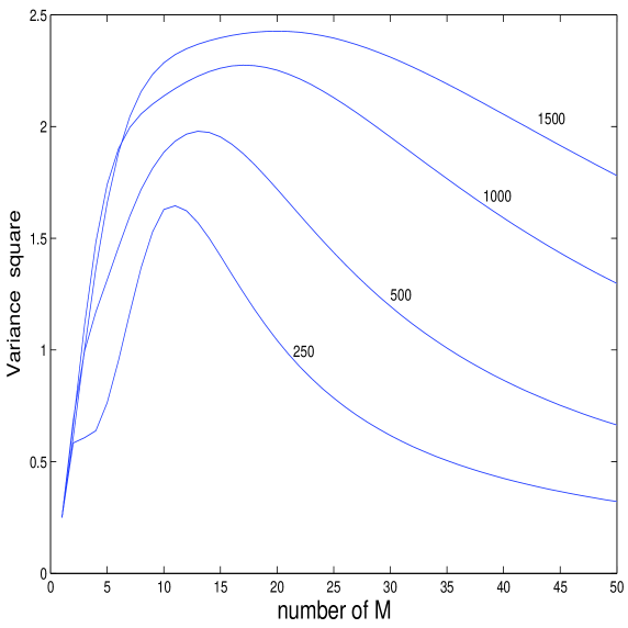
Figure 3: The variance square equal to $\sigma^{2}_{S}(M)$, for various values of the backward binding rate $k_{-1}=[250,500,1000,1500]$. The total number of substrate molecules is fixed at $S=10$ and $\tau=0.01ms$.

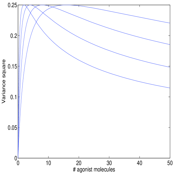
Figure 4: Normalized variance $\sigma^{2}$, for $\frac{k_{1}\Delta\mbox{\boldmath$x$}}{N_{S}k_{-1}}=$ 1/2, 1 ,2 ,4

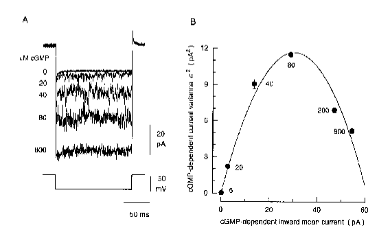
Figure 5: Experimental analysis of the fluctuation in the number of open channel. The left panel corresponds to the current response for various concentration of the gating molecules(cGMP), in a detached patch experiment of a cone Photoreceptors membrane. On the right panel, the variance is plotted versus the mean current, which is proportional to the number of gating molecules(cGMP). This picture was published in [18] figure 2.

References

- [1] J. Lisman, “The CaM kinase II hypothesis for the storage of synaptic memory”, Trends Neurosci. 10, pp.406-12 (1994).
- [2] F. Rieke and D.A. Baylor. 1996. Molecular origin of continuous dark noise in rod photoreceptors. Biophys J 71:2553-72.
- [3] S. Karlin and H. Taylor, A Second Course in Stochastic Processes, Academic Press, New York-London, 1981
- [4] L. Kleinrock and R. Gail, Queueing Systems. Problems and Solutions, Wiley-Interscience Publication. John Wiley Sons, Inc., New York, 1996.
- [5] D. Holcman, E. Korkotian, Z. Schuss, “Calcium dynamics in dendritic spines and spine motility”, Biophys. J 87, pp.81-91, (2004).
- [6] D. Holcman and J.I. Korenbrot, “Longitudinal diffusion in retinal rod and cone outer segment cytoplasm: the consequence of cell structure”, Biophys. J. 86 (4), pp.2566-82 (2004).
- [7] D. Holcman and Z. Schuss, “Kinetics of non-arrhenius reactions”, (pre-print).
- [8] D. Holcman and Z. Schuss, “Modeling calcium dynamics in dendritic spines”, to appear in SIAM of Applied Mathematics .
- [9] D. Holcman and Z. Schuss, “Escape through a small opening: receptor trafficking in a synaptic membrane”, to appear in Journal of Statistical Physics.
- [10] B. Nadler, T. Naeh, Z. Schuss, “The stationary arrival process of independent diffusers from a continuum to an absorbing boundary is Poissonian”. SIAM J. Appl. Math. 62, pp.433–447 (2001).
- [11] D. Holcman, A. Marchewka, Z. schuss, “The survival probability of diffusion with killing”, submitted.
- [12] P. Hänggi, P. Talkner, M. Borkovec, “Reaction rate theory: fifty years after Kramers”, Rev. Mod. Phys. 62 (2), pp.251-341 (1990).
- [13] B.J. Matkowsky and Z. Schuss, “The exit problem for randomly perturbed dynamical systems”, SIAM J. Appl. Math. 33, pp.367-382 (1977).
- [14] B.J. Matkowsky, Z. Schuss, E. Ben-Jacob, “A singular perturbation approach to Kramers’ diffusion problem”, SIAM J. Appl. Math. 42 (2), pp.835-849, (1982).
- [15] T. Naeh, M.M. Kłosek, B.J. Matkowsky, Z. Schuss, “A direct approach to the exit problem”, SIAM J. Appl. Math. 50 (2), pp.595-627, (1990).
- [16] L.W. Haynes, A.R. Kay, K.W. Yau, “Single cyclic GMP-activated channel activity in excised patches of rod outer segment membrane”, Nature 321 (6065) May 1-7, pp.66-70, (1986).
- [17] G. Matthews, “Comparison of the light-sensitive and cyclic GMP-sensitive conductances of the rod photoreceptor: noise characteristics”, J Neurosci. 6 (9), pp.2521-6, (1986).
- [18] A. Picones , J.I. Korenbrot, “Analysis of fluctuations in the cGMP-dependent currents of cone photoreceptor outer segments”, Biophys. J. 66 (2 Pt 1), pp.360-5, (1994).
- [19] F.J. Sigworth, “The variance of sodium current fluctuations at the node of Ranvier”, J. Physiol. (1980).
- [20] A. Singer, Z.Schuss, B. Nadler, R. Eisenberg, Models of boundary behavior of particles diffusing between two concentrations (pre-print).
- [21] Z. Schuss, Theory and Applications of Stochastic Differential Equations, Wiley Series in Probability and Statistics. John Wiley Sons, Inc., New York, 1980
- [22] T.L. Saaty, Elements of Queuing Theory With Applications, Dover NY, 1983.