Comparison of alternative improved perturbative methods for nonlinear oscillations

Abstract

We discuss and compare two alternative perturbation approaches for the calculation of the period of nonlinear systems based on the Lindstedt–Poincaré technique. As illustrative examples we choose one–dimensional anharmonic oscillators and the Van der Pol equation. Our results show that each approach is better for just one type of model considered here.

1 Introduction

There are several methods for removing the secular terms produced by the straightforward application of perturbation theory to nonlinear motion [1]. One of them is the Lindstedt–Poincaré technique (LPT) [1, 2], recently improved by Amore et al. [3, 4, 5, 6] by means of the delta expansion and the principle of minimal sensitivity (PMS) [7] giving rise to the LPLDE method.

There is also another approach that resembles the LPT [8] that we will call alternative Lindstedt–Poincaré technique (ALPT) from now on. The purpose of this letter is the discussion of those alternative approaches and comparison of their results for simple nontrivial models.

In Sec. 2 we briefly review the LPT [1, 2] and the LPLDE [3, 4, 5, 6]. In Sec. 3 we outline the ALPT [8]. In all those cases we choose the Duffing oscillator [1] as an illustrative example. In Sec. 4 we apply the LPLDE and the ALPT to other anharmonic oscillators. In Sec. 5 we apply both methods to the Van der Pol equation. Finally, in Sec. 6 we compare the frequencies of the motion for the above mentioned models calculated with both approaches.

2 The Lindstedt-Poincaré Technique

The LPT consists of the simultaneous expansion of the trajectory and oscillation frequency in powers of the perturbation parameter. For concreteness we choose the Duffing anharmonic oscillator as an illustrative example, [1]:

$$\frac{d^{2}x(t)}{dt^{2}}+x(t)=-\mu x^{3}(t)\ ,$$ (1)

with the initial conditions $x(0)=1$ and $\frac{dx(0)}{dt}=0$. The parameter $\mu$ is a measure of the nonlinearity of the motion.

Straightforward application of perturbation theory to Eq. (1) produces an approximate solution in the form of a $\mu$–power series $x(t)=\sum_{n=0}^{\infty}x_{n}(t)\mu^{n}$ [1, 2]. It is well–known that the equations for the coefficients $x_{n}(t)$ have resonant terms that after integration give rise to nonperiodic contributions [1, 2]. Such terms are unbounded in spite of the fact that the solution $x(t)$ is known to be periodic for all $\mu>-1$. For this reason, the perturbative solution fails at large time scales.

There are several approaches that provide approximate solutions free from secular terms [1]. Here we are interested in the Lindstedt–Poincaré technique that consists of introducing the actual frequency of motion $\Omega$ into the equation of motion by means of a time dilatation $\tau=\Omega t$ [1, 2]. Thus the Duffing equation (1) becomes

$$\Omega^{2}\ddot{X}(\tau)+X(\tau)=-\mu X^{3}(\tau),$$ (2)

where $X(\tau)\equiv x(\tau/\Omega)$ and the dot represents derivation with respect to $\tau$. Notice that the period of $X(\tau)$ is independent of $\mu$. On expanding both $X(\tau)$ and $\Omega^{2}$ in powers of $\mu$,

$$\Omega^{2}=\sum_{n=0}^{\infty}\alpha_{n}\mu^{n}\;,\qquad X(\tau)=\sum_{n=0}^{\infty}X_{n}(\tau)\mu^{n}\;,$$ (3)

with $\alpha_{0}=1$, one obtains the set of equations

$$\ddot{X}_{n}(\tau)+X_{n}(\tau) = -\theta(n-1)\left[\sum_{j=0}^{n-1}\sum_{k=0}^{n-1-j}X_{j}(\tau)X_{k}(\tau)X_{n-1-j-k}(\tau)\right.\$$

$$\left.+\sum_{j=1}^{n}\alpha_{j}\ddot{X}_{n-j}(\tau)\right]$$

$$n = 0,1,2,\ldots$$ (4)

where $\theta$ is the Heaviside function.

If we choose the coefficients $\alpha_{n}$ in order to remove the resonant terms, then the solutions $X_{n}(\tau)$ are periodic, have the general form

$$X_{n}(\tau)=\sum_{j=0}^{n}A_{nj}\cos{[(2j+1)\tau]}\;,$$ (5)

and satisfy the initial conditions

$$X_{n}(0)=\delta_{n0},\,\dot{X}_{n}(0)=0\ .$$ (6)

This approach not only gives us a truly periodic approximate solution but also the frequency of the motion in the form of a power series. For example, through third order we have:

$$\Omega_{(3)}^{2}=1+\frac{3}{4}\mu-\frac{3}{128}\mu^{2}+\frac{9}{512}\mu^{3}\;.$$ (7)

Since the motion is unbounded for $\mu<-1$ then the $\mu$–power series is expected to be valid only for $|\mu|<1$. This is a serious limitation of the LPT because the motion is periodic for all $\mu>-1$ as indicated above.

2.1 The Lindstedt–Poincaré Technique and the Linear Delta Expansion

In order to improve the LPT, Amore et al. [3, 4, 5, 6] proposed its combination with the linear delta expansion (LDE). The LDE is a variational perturbation theory like the one proposed some time ago as a renormalization of the perturbation series in quantum mechanics [9] which has proved being suitable for the treatment of a wide variety of problems [2, 10].

In order to apply the LDE to the Duffing oscillator we rewrite Eq. (1) as

$$\frac{d^{2}x(t)}{dt^{2}}+\left(1+\lambda^{2}\right)x(t)=\delta\left[-\mu x^{3}(t)+\lambda^{2}x(t)\right]$$ (8)

where $\lambda$ is a variational parameter and $\delta$ is an order–counting parameter. When we set $\delta$ equal to one we recover the original equation (1) that is independent of $\lambda$. Following the LPT outlined above we change the time variable and obtain

$$\Omega^{2}\ddot{X}(\tau)+(1+\lambda^{2})X(\tau)=\delta\left[-\mu X^{3}(\tau)+\lambda^{2}X(\tau)\right].$$ (9)

Next we expand both $X$ and $\Omega^{2}$ in powers of $\delta$ and proceed exactly as indicated above for the Lindstedt–Poincaré technique, except that in this case we choose $\alpha_{0}=1+\lambda^{2}$. The resulting perturbation equation of order $n$ reads

$$\ddot{X}_{n}(\tau)+X_{n}(\tau) = -\frac{\theta(n-1)}{\alpha_{0}}\left[\sum_{j=0}^{n-1}\sum_{k=0}^{n-1-j}X_{j}(\tau)X_{k}(\tau)X_{n-1-j-k}(\tau)\right.\;$$

$$+\left.\sum_{j=1}^{n}\alpha_{j}\ddot{X}_{n-j}(\tau)-\lambda^{2}X_{n-1}(\tau)\right],$$

$$n = 0,1,\ldots$$ (10)

and the solutions satisfy the initial conditions (6). As before, the coefficient $\alpha_{n}$ is set to remove the resonant term from the equation of order $n$. At third order we find, after setting $\delta=1$,

$$\Omega_{(3)}^{2}=1+\frac{3\mu}{4}-\frac{3\mu^{2}}{128(1+\lambda^{2})}+\frac{3\mu^{2}(3\mu-4\lambda^{2})}{512(1+\lambda^{2})^{2}}\;.$$ (11)

We assume that the optimum value of the arbitrary variational parameter $\lambda$ is given by the principle of minimal sensitivity (PMS) [7]

$$\frac{d\Omega_{(N)}}{d\lambda}=0\;$$ (12)

that gives us $\lambda_{PMS}^{(N)}$ and an approximate expression of order $N$. At third order we have

$$\lambda_{PMS}^{(3)}=\frac{\sqrt{3\mu}}{2}$$ (13)

and the approximate frequency results to be

$$\Omega_{(3)}^{2}=\frac{69\mu^{2}+192\mu+128}{32(3\mu+4)}\;.$$ (14)

We have already named this approach Lindstedt–Poincaré–Linear–Delta–Expansion (LPLDE).

The LPLDE approximants are not $\mu$–power series and prove to be valid for all $\mu>-1$.

3 Alternative Lindstedt–Poincaré Technique

There is another approach that resembles the LPT discussed above that consists of rewriting Eq. (1) as [8]

$$\frac{d^{2}x(t)}{dt^{2}}+\left(\Omega^{2}-\sum_{n=1}^{\infty}\alpha_{n}\mu^{n}\right)x(t)=-\mu x^{3}(t)\;.$$ (15)

Expanding $x(t)$ in a $\mu$–power series and considering $\Omega$ independent of this parameter, the perturbative equation of order $n$ becomes

$$\frac{d^{2}x_{n}(t)}{dt^{2}}+\Omega^{2}x_{n}(t) = -\theta(n-1)\left[\sum_{j=0}^{n-1}\sum_{k=0}^{n-1-j}x_{j}(t)x_{k}(t)x_{n-1-j-k}(t)\right.\;$$ (16)

$$\left.+\sum_{j=0}^{n}\alpha_{j}x_{n-j}(t)\right].$$

The general form of the solutions $x_{n}(t)$ which fulfill the initial conditions (6) is

$$x_{n}(t)=\sum_{j=0}^{n}A_{nj}\cos{[(2j+1)\Omega t]}\;,$$ (17)

provided that the coefficients $\alpha_{n}$ remove the resonant terms. These coefficients turn out to depend upon $\Omega$ and, as a result, any truncated expansion for $\Omega^{2}$ is a self–consistent equation for the frequency. For example, solving for $\Omega_{(3)}^{2}$ in the equation of third order

$$\Omega_{(3)}^{2}=1+\frac{3\mu}{4}-\frac{3\mu^{2}}{128\Omega_{(3)}^{2}}+0\mu^{3}\;,$$ (18)

we obtain

$$\Omega_{(3)}^{2}=\frac{\sqrt{30\mu^{2}+96\mu+64}+2(3\mu+4)}{16}\;.$$ (19)

We have earlier called this approximation ALPT.

4 Other Anharmonic Potentials

In order to compare the approaches outlined above we also consider anharmonic oscillators with potentials

$$V(x)=\frac{1}{2}x^{2}+\frac{\mu}{2N}x^{2N}\;,\;N=2,3,\ldots$$ (20)

that lead to the equations of motion

$$\frac{d^{2}x(t)}{dt^{2}}+x(t)=-\mu x^{2N-1}\;,$$ (21)

with exactly the same initial conditions considered before for the Duffing oscillator, which is a particular case with $N=2$. Notice that there is periodic motion for all $\mu>-1$ consistent with the initial conditions.

Here we apply the LPLDE and the ALPT to the cases $N=3$ and $N=4$. The procedure is straightforward, and we only remark that after removal of resonant terms the general form of the LPT and LPLDE solutions is

$$X_{n}(\tau)=\sum_{j=0}^{Nn}A_{nj}\cos{[(2j+1)\tau]}\;,$$ (22)

whereas for the ALPT we have

$$x_{n}(t)=\sum_{j=0}^{Nn}A_{nj}\cos{[(2j+1)\Omega t]}\;.$$ (23)

5 The Van der Pol equation

In order to test the performance of the approaches outlined above we also choose the well–known Van der Pol (VdP) equation

$$\frac{d^{2}x(t)}{dt^{2}}+x(t)=\mu\ [1-x^{2}(t)]\ \frac{dx(t)}{dt}.$$ (24)

because the behaviour of its solutions is completely different from those of the anharmonic oscillators discussed above.

The VdP equation exhibits a limit cycle and leads to oscillations with a definite period that depends on the coupling $\mu$. However, unlike the anharmonic oscillators the VdP equation does not correspond to a conservative system as the driving term either damps or enhances the oscillation depending upon the size of $x$. This equation has already been treated by means of the LPLDE approach  [6]; here we apply and compare it with the ALP method.

5.1 The LPLDE Technique

We first rewrite the VdP equation (24) as [6]

$$\Omega^{2}\ddot{x}(\tau)+(1+\lambda^{2})x(\tau)=\delta\{\mu\Omega[1-x^{2}(\tau)]\dot{x}(\tau)+\lambda^{2}x(\tau)\}\;.$$ (25)

In this case we expand $\Omega$ (instead of $\Omega^{2}$) in powers of $\delta$

$$\Omega=\sum_{n=0}^{\infty}\alpha_{n}\delta^{n}\ \ \ ,\ \ \ x=\sum_{n=0}^{\infty}x_{n}(\tau)\delta^{n}\;,$$ (26)

and choose $\alpha_{0}=1+\lambda^{2}$. We thus obtain

$$\ddot{x}_{n}(\tau)+x_{n}(\tau) = \frac{\theta(n-1)}{\alpha_{0}}\left[\mu\sum_{j=0}^{n-1}\alpha_{j}\dot{x}_{n-1-j}-\sum_{j=1}^{n}\alpha_{j}\ddot{x}_{n-j}(\tau)\right.$$ (27)

$$\left.-\mu\sum_{i=0}^{n-1}\sum_{j=0}^{n-1-i}\sum_{k=0}^{n-1-i-j}\alpha_{i}x_{j}(\tau)x_{k}(\tau)\dot{x}_{n-1-i-j-k}(\tau)\right].$$

The general form of the solutions is

$$x_{n}(\tau)=\sum_{j=0}^{n}\left[c_{nj}\cos(2j+1)\tau+d_{nj}\sin(2j+1)\tau\right]\ ,$$ (28)

that satisfy the initial conditions

$$x_{n}(0)=A_{n}\ \ \ ,\ \ \ \dot{x}_{n}(0)=0$$ (29)

for $n\geq 1$. The appropriate choice of $\alpha_{n}$ and $A_{n-1}$ enables us to remove all resonant terms at order $n$.

5.2 The ALPT

Proceeding as in the case of the anharmonic oscillators we substitute the expansion for the frequency $\Omega^{2}$ into the VdP equation and obtain

$$\frac{d^{2}x_{n}(t)}{dt^{2}}+\Omega^{2}x_{n}(t) = \theta(n-1)\left[\sum_{j=1}^{n}\alpha_{j}x_{n-j}(t)+\frac{dx_{n-1}(t)}{dt}\right.$$ (30)

$$\left.-\sum_{j_{1}=0}^{n-1}\sum_{j_{2}=0}^{n-1-j_{1}}x_{j_{1}}(t)\ x_{j_{2}}(t)\ \frac{dx_{n-1-j_{1}-j_{2}}(t)}{dt}\right]$$

The general form of the solutions in this case is

$$x_{n}(t)=\sum_{j=0}^{n}\left\{c_{nj}\cos[(2j+1)\Omega t]+d_{nj}\sin[(2j+1)\Omega t]\right\}\ ,$$ (31)

that satisfy the initial conditions (29).

The appropriate choice of $\alpha_{n}$ and $A_{n-1}$ enable us to remove secular terms at order $n$. As before, the coefficients $\alpha_{n}$ of the expansion of $\Omega^{2}$ in powers of $\mu$ depend on $\Omega$ that one obtains as a real solution of the partial sum at a given order.

6 Results and Discussion

We first consider the results of the LPLDE and ALPT for the Duffing oscillator. In the case of the LPLDE we use at all orders the variational parameter $\lambda_{PMS}$ calculated at third order. Fig. (1) shows the error over the frequency, defined as $\Delta\equiv|\Omega_{exact}-\Omega_{approx}|$, as a function of $\mu$ ($\mu\geq 0$) produced by partial sums through order $20$ for both approaches. We observe that the LPLDE technique, which yields much more accurate results than the straightforward LPT, is less accurate than the ALPT. A similar behavior can be observed in Fig. (2), where the error over the frequency is plotted for $-1\leq\mu\leq 0$. Interestingly, close to $\mu=-1$, which corresponds to a condition of (unstable) equilibrium, the LPLDE method performs better than the ALPT.

Similar conclusions can be drawn in the case of anharmonic oscillators with greater $N$. Figs. (3) and (4) show the error over the frequency as a function of the order of approximation for quartic (Duffing), sextic and octic anharmonic oscillators with $\mu=1$ and $\mu=100$, respectively.

The situation is different in the case of the nonconservative VdP equation because the ALPT exhibits a great convergence rate, but it yields a wrong frequency for $\mu>\simeq 2$, which suggests a wrong dependence on this coupling parameter. On the other hand, the LPLDE yields reasonable results for any value of $\mu$, as shown in Fig. (5).

Our results suggest that the ALPT method is more accurate for conservative systems but fails for nonconservative ones, while, on the other hand, the LPLDE yields reasonable results in both cases. At present we are unable to explain the failure of the ALPT for nonconservative systems and we believe that this subject deserves further investigation.

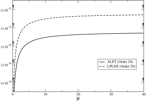
Figure 1: Error over the frequency as a function of $\mu$.

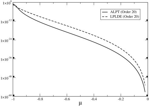
Figure 2: Error over the frequency as a function of $\mu$, for $-1\leq\mu\leq 0$.

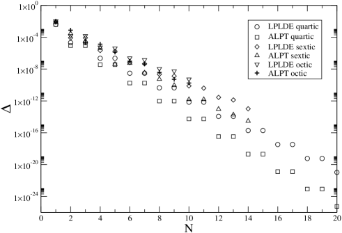
Figure 3: Error over the frequency as a function of the number of terms taking $\mu=1$ for different anharmonic potentials.

Figure 4: Error over the frequency as a function of the number of terms taking $\mu=100$ for different anharmonic potentials.

Figure 5: Period of the Van der Pol oscillator as a function of $\mu$.

Acknowledgements P.A. acknowledges support of Conacyt grant no. C01-40633/A-1. P.A. and A.R. acknowledge support of the Alvarez-Buylla fund of the University of Colima.

References

- [1] A. H. Nayfeh, Introduction to Perturbation Techniques (John Wiley & Sons, New York, 1981).
- [2] F. M. Fernández, Introduction to Perturbation Theory in Quantum Mechanics (CRC Press, Boca Raton, 2000).
- [3] P. Amore and A. Aranda, Phys. Lett. A 316, 218 (2003).
- [4] P. Amore and H. Montes Lamas, Phys. Lett. A 327, 158 (2004).
- [5] P. Amore and A. Aranda, Preprint math-ph/0303052.
- [6] P. Amore and H. Montes, Phys. Lett. A (in press), Preprint math-ph/0310060.
- [7] P. M. Stevenson, Phys. Rev. D 23, 2916 (1981).
- [8] J. Marion, Classical Dynamics of Particles and Systems, Second ed. (Academic, New York, 1970).
- [9] J. Killingbeck, J. Phys. A 14, 1005 (1980).
- [10] G. A. Arteca, F. M. Fernández, and E. A. Castro, Large order perturbation theory and summation methods in quantum mechanics (Springer, Berlin, Heidelberg, New York, London, Paris, Tokyo, Hong Kong, Barcelona, 1990).
- [11] M. P. Blencowe and A. P. Korte, Phys. Rev. B 56 9422 (1997).
- [12] H. F. Jones, P. Parkin and D. Winder, Phys. Rev. D 63, 125013 (2001).
- [13] J. L. Kneur, M. B. Pinto and R. O. Ramos, Preprint cond-mat/0207295.
- [14] J. L. Kneur, M. B. Pinto and R. O. Ramos, Phys. Rev. Lett. 89 210403 (2002). Preprint cond-mat/0207295.
- [15] G. Krein, D. P. Menezes and M. B. Pinto, Phys. Lett. B 370 5 (1996).
- [16] M. B. Pinto and R. O. Ramos, Phys. Rev. D 60 105005 (1999).
- [17] A. Okopińska, Phys. Rev. D 35, 1835 (1987); A. Duncan and M. Moshe, Phys. Lett. B 215, 352 (1988).