On convergence towards a self-similar solution for a nonlinear wave equation - a case study

Abstract

We consider the problem of asymptotic stability of a self-similar attractor for a simple semilinear radial wave equation which arises in the study of the Yang-Mills equations in 5+1 dimensions. Our analysis consists of two steps. In the first step we determine the spectrum of linearized perturbations about the attractor using a method of continued fractions. In the second step we demonstrate numerically that the resulting eigensystem provides an accurate description of the dynamics of convergence towards the attractor.

1 Introduction

Self-similar solutions of evolution equations often appear as attractors in a sense that solutions of an initial value problem starting from generic initial data evolve asymptotically into a self-similar form. In such cases one would like to describe the process of convergence to the self-similar solution and understand the mechanism responsible for this phenomenon. These kind of problems are relatively well-understood for diffusion equations where the global dissipation of energy is the mechanism of convergence to an attractor, however very little is known for conservative wave equations where the local dissipation of energy is due to dispersion. In this paper we report on analytical and numerical studies of this problem for a semilinear radial wave equation of the form

$$u_{tt}-u_{rr}-\frac{2}{r}u_{r}+\frac{f(u)}{r^{2}}=0,$$ (1)

where $r$ is the radial variable, $u=u(t,r)$, and $f(u)=-3u(1-u^{2})$. This equation appears in the study of the spherically symmetric Yang-Mills equations in $5+1$ dimensions (see [2] for the derivation). We remark in passing that our results hold for more general nonlinearities, in particular for $f(u)=\sin(2u)$ which corresponds to the equivariant wave maps from the $3+1$ dimensional Minkowski spacetime into the three-sphere.

It was proved in [1] and later found explicitly in [2] that equation (1) has a self-similar solution

$$u(t,r)=U_{0}(\rho)=\frac{1-\rho^{2}}{1+\frac{3}{5}\rho^{2}},$$ (2)

where $\rho=r/(T-t)$ is a similarity variable and $T>0$ is a constant (actually, $U_{0}$ is the ground state of a countable family of self-similar solutions $U_{n}$ ($n=0,1,\dots$) but since all $n>0$ solutions are unstable they do not appear as attractors for generic initial data). Since

$$\partial_{r}^{2}U_{0}(\rho)\Bigr{\rvert}_{r=0}\sim\frac{1}{(T-t)^{2}},$$ (3)

the solution $U_{0}(\rho)$ becomes singular at the center when $t\rightarrow T$. By the finite speed of propagation, one can truncate this solution in space to get a smooth solution with compactly supported initial data which blows up in finite time.

In fact, the self-similar solution $U_{0}$ is not only an explicit example of singularity formation, but more importantly it appears as an attractor in the dynamics of generic initial data. We conjectured in [3] that generic solutions of equation (1) starting with sufficiently large initial data do blow up in a finite time in the sense that $u_{rr}(t,0)$ diverges at $t\nearrow T$ for some $T>0$ and the asymptotic profile of blowup is universally given by $U_{0}$, that is

$$\lim_{t\nearrow T}u(t,(T-t)r)=U_{0}(r).$$ (4)

Figure 1 shows the numerical evidence supporting this conjecture.

Figure 1: The upper plot shows the late time evolution of some large initial data which blow up at time $T$. As the blowup progresses, the inner solution gradually attains the form of the stable self-similar solution $U_{0}(r/(T-t))$. The outer solution appears frozen on this timescale. In the lower plot the rescaled solutions $u(t,(T-t)r)$ are shown to collapse to the profile $U_{0}(r)$ (solid line).

The goal of this paper is to describe in detail how the limit (4) is attained. To this end, in section 2 we first study the linear stability of the solution $U_{0}$. This leads to an eigenvalue problem which is rather unusual from the standpoint of spectral theory of linear operators. We solve this problem in section 3 using the method of continued fractions. Then, in section 4 we present the numerical evidence that the deviation of the dynamical solution from the self-similar attractor is asymptotically well described by the least damped eigenmode.

2 Linear stability analysis

The role of the self-similar solution $U_{0}$ in the evolution depends crucially on its stability with respect to small perturbations. In order to analyze this problem it is convenient to define the new time coordinate $\tau=-\ln(T-t)$ and rewrite equation (1) in terms of $U(\tau,\rho)=u(t,r)$

$$U_{\tau\tau}+U_{\tau}+2\rho\>U_{\rho\tau}-(1-\rho^{2})(U_{\rho\rho}+\frac{2}{\rho}U_{\rho})+\frac{f(U)}{\rho^{2}}=0.$$ (5)

In these variables the problem of finite time blowup in converted into the problem of asymptotic convergence for $\tau\rightarrow\infty$ towards the stationary solution $U_{0}(\rho)$. Following the standard procedure we seek solutions of equation (5) in the form $U(\tau,\rho)=U_{0}(\rho)+w(\tau,\rho)$. Neglecting the $O(w^{2})$ terms we obtain a linear evolution equation for the perturbation $w(\tau,\rho)$

$$w_{\tau\tau}+w_{\tau}+2\rho\>w_{\rho\tau}-(1-\rho^{2})(w_{\rho\rho}+\frac{2}{\rho}w_{\rho})+\frac{f^{\prime}(U_{0})}{\rho^{2}}w=0.$$ (6)

Substituting $w(\tau,\rho)=e^{\lambda\tau}v(\rho)/\rho$ into (6) we get the eigenvalue equation

$$-(1-\rho^{2})v^{\prime\prime}+2\lambda\rho v^{\prime}+\lambda(\lambda-1)v+\frac{V(\rho)}{\rho^{2}}v=0,$$ (7)

where

$$V(\rho)=f^{\prime}(U_{0})=\frac{6(25-90\rho^{2}+33\rho^{4})}{(5+3\rho^{2})^{2}}.$$ (8)

We consider equation (7) on the interval $0\leq\rho\leq 1$, which corresponds to the interior of the past light cone of the blowup point $(t=T,r=0)$. Since a solution of the initial value problem for equation (1) starting from smooth initial data remains smooth for all times $t<T$, we demand the solution $v(\rho)$ to be analytic at the both endpoints $\rho=0$ (the center) and $\rho=1$ (the past light cone). Such a globally analytic solution of the singular boundary value problem can exist only for discrete values of the parameter $\lambda$, hereafter called eigenvalues. In order to find the eigenvalues we apply the method of Frobenius.

The indicial exponents at the regular singular point $\rho=0$ are $3$ and $-1$, hence the solution which is analytic at $\rho=0$ has the power series representation

$$v_{0}(\rho)=\sum_{n=0}^{\infty}a_{n}(\lambda)\rho^{2n+3},\qquad a_{0}\neq 0.$$ (9)

Since the nearest singularity in the complex $\rho$-plane is at $\rho=1$, the series (9) is absolutely convergent for $0\leq\rho<1$. At the second regular singular point, $\rho=1$, the indicial exponents are $0$ and $1-\lambda$ so, as long as $\lambda$ is not an integer, the two linearly independent solutions have the power series representations

$$v_{1}(\rho)=\sum_{n=0}^{\infty}b_{n}^{(1)}(\lambda)(1-\rho)^{n},\qquad v_{2}(\rho)=\sum_{n=0}^{\infty}b_{n}^{(2)}(\lambda)(1-\rho)^{n+1-\lambda}.$$ (10)

These series are absolutely convergent for $0<\rho\leq 1$. If $\lambda$ is not an integer, only the solution $v_{1}(\rho)$ is analytic at $\rho=1$. From the theory of linear ordinary differential equations we know that the three solutions $v_{0}(\rho)$, $v_{1}(\rho)$, and $v_{2}(\rho)$ are connected on the interval $0<\rho<1$ by the linear relation

$$v_{0}(\rho)=A(\lambda)v_{1}(\rho)+B(\lambda)v_{2}(\rho).$$ (11)

The requirement that the solution which is analytic at $\rho=0$ is also analytic at $\rho=1$ serves as the quantization condition for the eigenvalues $B(\lambda)=0$. Unfortunately, the explicit expressions for the connection coefficients $A(\lambda)$ and $B(\lambda)$ are not known for equations with more than three regular singular points. There are, however, other indirect methods of solving the equation $B(\lambda)=0$. One of them is a shooting method which goes as follows. One approximates the solutions $v_{0}(\rho)$ and $v_{1}(\rho)$ by the power series (9) and (10), respectively, truncated at some sufficiently large $n$, and then computes the Wronskian of these solutions at midpoint, $\rho=1/2$, say. The zeros of the Wronskian correspond to the eigenvalues (see figure 2). Although this method gives the eigenvalues with reasonable accuracy, it is computationally very costly, especially for large negative values of $\lambda$, because the power series (9) and (10) converge very slowly. We point out that shooting towards $\rho=1$ fails completely for large negative $\lambda$ because the solution $v_{2}(\rho)$ is subdominant at $\rho=1$, that is, it is negligible with respect to the analytic solution $v_{1}(\rho)$.

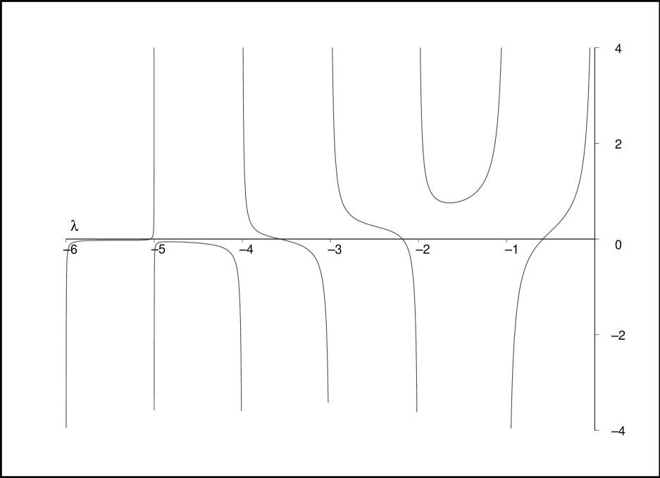
Figure 2: The Wronskian $W[v_{0},v_{1}](\rho=1/2,\lambda)$.

3 The continued fractions method

In this section we shall solve the eigenvalue problem (7) using a method continued fractions. The key idea is to determine the analyticity properties of the power series solution $v_{0}(\rho)$ from the asymptotic behavior of the expansion coefficients $a_{n}$. Substituting the power series (9) into equation (7) we get the four-term recurrence relation (with the initial conditions $a_{0}=1$ (normalization) and $a_{n}=0$ for $n<0$)

$$p_{3}(n)a_{n+3}+p_{2}(n)a_{n+2}+p_{1}(n)a_{n+1}+p_{0}(n)a_{n}=0,$$ (12)

where

$$p_{3}(n) = -100n^{2}-850n-1650,$$

$$p_{2}(n) = -20n^{2}+(100\lambda-130)n+\!25\lambda^{2}+325\lambda-750,$$

$$p_{1}(n) = 84n^{2}+(120\lambda+378)n+30\lambda^{2}+270\lambda+618,$$

$$p_{0}(n) = 36n^{2}+(36\lambda+90)n+9\lambda^{2}+45\lambda+54.$$

For $n=-2$ we have

$$-350a_{1}+(25\lambda^{2}+125\lambda-570)a_{0}=0,$$ (13)

and for $n=-1$

$$-900a_{2}+(25\lambda^{2}+225\lambda-640)a_{1}+(30\lambda^{2}+150\lambda+324)a_{0}=0.$$ (14)

The series (9) is absolutely convergent for $0\leq\rho<1$ and in general is divergent for $\rho>1$. In order to determine the analyticity properties of the solution $v_{0}(\rho)$ at $\rho=1$ we need to find the large $n$ behavior of the expansion coefficients $a_{n}$. The four-term recurrence relation (12) can be viewed as the third order difference equation so it has three linearly independent asymptotic solutions for $n\rightarrow\infty$. Following standard methods (see, for example, [4]) we find

$$a_{n}^{(1)}\sim n^{\lambda-2}\sum_{s=0}^{\infty}\frac{\alpha_{s}^{(1)}}{n^{s}},\qquad a_{n}^{(2)}\sim\left(-\frac{3}{5}\right)^{n}n\sum_{s=0}^{\infty}\frac{\alpha_{s}^{(2)}}{n^{s}},\qquad a_{n}^{(3)}\sim\left(-\frac{3}{5}\right)^{n}n^{-4}\sum_{s=0}^{\infty}\frac{\alpha_{s}^{(3)}}{n^{s}}.$$ (15)

Thus, in general, the solution of the recurrence relation (12) behaves asymptotically as

$$a_{n}\sim c_{1}(\lambda)a_{n}^{(1)}+c_{2}(\lambda)a_{n}^{(2)}+c_{3}(\lambda)a_{n}^{(3)}.$$ (16)

If the coefficient $c_{1}(\lambda)$ is nonzero then

$$\frac{a_{n+1}}{a_{n}}\sim\frac{a^{(1)}_{n+1}}{a^{(1)}_{n}}\rightarrow 1\quad\text{as}\quad n\rightarrow\infty,$$ (17)

hence the power series (9) is divergent for $\rho>1$ (in fact it has a branch point singularity at $\rho=1$). On the other hand, if $c_{1}(\lambda)=0$ then the solution $v_{0}(\rho)$ can be continued analytically through $\rho=1$. The advantage of replacing the quantization condition $B(\lambda)=0$ in the connection formula (11) by the equivalent condition $c_{1}(\lambda)=0$ follows from the fact that $c_{1}(\lambda)$ is the coefficient of the dominant solution in (16), in contrast to $B(\lambda)$ which is the coefficient of the subdominant solution in (11).

Now, we shall find the zeros of the coefficient $c_{1}(\lambda)$ using the method of continued fractions. This method is based on an intimate relationship between three-term recurrence relations and continued fractions. It goes as follows. Suppose that we have a three-term recurrence relation (a second order difference equation)

$$b_{n+2}+A_{n}b_{n+1}+B_{n}b_{n}=0.$$ (18)

Let $r_{n}=b_{n+1}/b_{n}$. Then, from (18) we have

$$r_{n}=-\frac{B_{n}}{A_{n}+r_{n+1}},$$

and applying this formula repeatedly we get the continued fraction representation of $r_{n}$

$$r_{n}=-\frac{B_{n}}{A_{n}-}\;\frac{B_{n+1}}{A_{n+1}-}\;\frac{B_{n+2}}{A_{n+2}-}...$$ (19)

A theorem due to Pincherle [4] says that the continued fraction on the right hand side of equation (19) converges if and only if the recurrence relation (18) has a minimal solution $b^{min}_{n}$, i.e. the solution such that $\lim_{n\rightarrow\infty}b^{min}_{n}/b_{n}=0$ for any other solution $b_{n}$. Moreover, in the case of convergence, equation (19) holds with $r_{n}=b^{min}_{n+1}/b^{min}_{n}$ for each $n$.

We cannot yet apply this theorem because our recurrence relation (12) has four terms. However, let us observe that

$$a_{n}=a_{n}^{exact}=\left(-\frac{3}{5}\right)^{n}\left[n+1+\frac{5}{16}(\lambda-1)\right]$$ (20)

is the exact solution of our four-term recurrence relation (12) (although it does not satisfy the initial conditions). Using this solution we can reduce the order by the substitution

$$b_{n}=a_{n+1}+\frac{3}{5}\frac{n+2+\frac{5}{16}(\lambda-1)}{n+1+\frac{5}{16}(\lambda-1)}\;a_{n}$$ (21)

to get the three-term recurrence relation

$$q_{2}(n)b_{n+2}+q_{1}(n)b_{n+1}+q_{0}(n)b_{n}=0,$$ (22)

where (using the abbreviation $\gamma=5(\lambda-1)/16$)

$$q_{0}(n) = p_{1}(n)-\frac{3}{5}\frac{n+3+\gamma}{n+2+\gamma}\,p_{2}(n)+\left(\frac{3}{5}\right)^{2}\frac{n+4+\gamma}{n+2+\gamma}\,p_{3}(n),$$

$$q_{1}(n) = p_{2}(n)-\frac{3}{5}\frac{n+4+\gamma}{n+3+\gamma}\,p_{3}(n),$$

$$q_{2}(n) = p_{3}(n).$$

The two linearly independent asymptotic solutions of the recurrence relation (22) are

$$b_{n}^{(1)}\sim n^{\lambda-2}\sum_{s=0}^{\infty}\frac{\beta_{s}^{(1)}}{n^{s}},\qquad a_{n}^{(2)}\sim\left(-\frac{3}{5}\right)^{n}n^{-5}\sum_{s=0}^{\infty}\frac{\beta_{s}^{(2)}}{n^{s}},$$ (23)

so in general

$$b_{n}\sim C_{1}(\lambda)b_{n}^{(1)}+C_{2}(\lambda)b_{n}^{(2)}.$$ (24)

Now, our quantization condition $c_{1}(\lambda)=0$ is equivalent to $C_{1}(\lambda)=0$ which is nothing else but the condition for the existence of a minimal solution for equation (22). Thus, we can use Pincherle’s theorem to find the eigenvalues.

In our case $A_{n}=q_{1}(n)/q_{2}(n)$ and $B_{n}=q_{0}(n)/q_{2}(n)$. From (13) and (21) we get

$$b_{0}=\left(\frac{25\lambda^{2}+125\lambda-570}{350}+\frac{96+15(\lambda-1)}{80+25(\lambda-1)}\right)a_{0},\qquad b_{-1}=a_{0}.$$ (25)

Using Pincherle’s theorem and setting $n=-1$ in (19) we obtain the eigenvalue equation

$$\frac{b_{0}}{b_{-1}}=\frac{25\lambda^{2}+125\lambda-570}{350}+\frac{96+15(\lambda-1)}{80+25(\lambda-1)}=-\frac{B_{-1}(\lambda)}{A_{-1}(\lambda)-}\;\frac{B_{0}(\lambda)}{A_{0}(\lambda)-}\;\frac{B_{1}(\lambda)}{A_{1}(\lambda)-}...$$ (26)

The continued fraction in (26), which by Pincherle’s theorem is convergent for any $\lambda$, can be approximated with essentially arbitrary accuracy by downward recursion starting from a sufficiently large $n=N$ and some (arbitrary) initial value $r_{N}$. The roots of the transcendental equation (26) are then found numerically (see table 1).

$$n$$

1 -0.588904 -2.181597 - 3.570756 - 5.043294 -6.486835

-7.912777 -9.298265 -9.907103 -10.792456 -12.153033 -13.164487

Table 1: The first twelve eigenvalues.

We recall from [2] that the eigenvalue $\lambda_{0}=1$ is due to the freedom of changing the blowup time $T$. Although this eigenvalue is positive, it should not be interpreted as the physical instability of the solution $U_{0}$ – it is an artifact of introducing the similarity variables and does not show up in the dynamics for $u(t,r)$. Note that, strangely enough, all the eigenvalues are real.

4 Convergence to the attractor

According to the linear stability analysis presented above the convergence of the solution $u(t,r)$ towards the self-similar attractor $U_{0}$ should be described by the formula

$$u(t,r)=U_{0}(\rho)+\sum_{k=1}c_{k}e^{\lambda_{k}\tau}v_{k}(\rho)/\rho\sim U_{0}(\rho)+c_{1}e^{\lambda_{1}\tau}v_{1}(\rho)/\rho\quad\text{as}\quad\tau\rightarrow\infty,$$ (27)

where $v_{k}(\rho)/\rho$ are the eigenmodes corresponding to the eigenvalues $\lambda_{k}$ and $c_{k}$ are the expansion coefficients. In order to verify the formula (27) we solved equation (1) numerically for large initial data leading to blowup, expressed the solution in the similarity variables, and computed the deviation from $U_{0}$ for $t\nearrow T$. Figure 4 shows that for small $T-t$ the deviation from $U_{0}$ is very well described by the least damped eigenmode $v_{1}$, in agreement with the formula (27). For larger $T-t$ the contribution of higher modes has to be included (see figure 5).

Figure 3: In this figure we determine the coefficient $c_{1}$ in the formula (27) as follows. Taking the second derivative of (27) at $r=0$ we obtain $(T-t)^{2}u_{rr}(t,r=0)+16/5=2c_{1}(T-t)^{-\lambda_{1}}$. For small $T-t$ we plot the left hand side of this equation in the log-log scale and fit the parameters $c_{1}$ and $\lambda_{1}$. We get $c_{1}=-0.031436$ and $\lambda_{1}=-0.58803$ (in good agreement with table 1).

Figure 4: We plot the deviation of the dynamical solution $u(t,r)$ from the self-similar solution $U_{0}$ at some moment of time close to the blowup time. The solid line shows the least damped eigenmode $c_{1}(T-t)^{-\lambda_{1}}v_{1}(\rho)/\rho$ with the coefficient $c_{1}$ obtained in figure 3.

Figure 5: The same plot as in figure 4 but at an earlier moment of time. The solid line showing the least damped eigenmode (with the same coefficient $c_{1}$ as before) does not fit well the numerical data because the other modes have not yet decayed. Including the suitably normalized second eigenfunction in the expansion (27) we get a much better fit (dashed line).

References

• [1] T. Cazenave, J. Shatah, and A. Shadi Tahvildar-Zadeh, Ann. Inst. Henri Poincare 68, 315 (1998).
• [2] P. Bizoń, Acta Phys. Polonica B 33, 1893 (2002).
• [3] P. Bizoń and Z. Tabor, Phys. Rev. D 64, 121701 (2001).
• [4] S. N. Elaydi, An Introduction to Difference Equations (Springer, 1999).