A tube formula for the Koch snowflake curve, with applications to complex dimensions.

Abstract

A formula for the interior $\varepsilon$-neighbourhood of the classical von Koch snowflake curve is computed in detail. This function of $\varepsilon$ is shown to match quite closely with earlier predictions from [La-vF1] of what it should be, but is also much more precise. The resulting ‘tube formula’ is expressed in terms of the Fourier coefficients of a suitable nonlinear and periodic analogue of the standard Cantor staircase function and reflects the self-similarity of the Koch curve. As a consequence, the possible complex dimensions of the Koch snowflake are computed explicitly.

1 Introduction

In [La-vF1], the authors lay the foundations for a theory of complex dimensions with a rather thorough investigation of the theory of fractal strings (see also, e.g., [LaPo1–2,LaMa,La1–3,HaLa,HeLa,La-vF2–3]); that is, fractal subsets of $\mathbb{R}$. Such an object may be represented by a sequence of bounded open intervals of length $l_{j}$:

$$\mathcal{L}:=\{l_{j}\}_{j=1}^{\infty},\quad\text{with }\sum_{j=1}^{\infty}l_{j}<\infty.$$ (1.1)

The authors are able to relate geometric and physical properties of such objects through the use of zeta functions which contain geometric and spectral information about the given string. This information includes the dimension and measurability of the fractal under consideration, which we now recall.

For a nonempty bounded open set $\Omega\subseteq\mathbb{R}$, $V(\varepsilon)$ is defined to be the inner $\varepsilon$-neighborhood of $\Omega$:

$$V(\varepsilon):=\operatorname{vol_{\text{$1$}}}\{x\in\Omega\rule{0.86108pt}{0.0pt}:\rule{0.86108pt}{0.0pt}d(x,\partial\Omega)<\varepsilon\},$$ (1.2)

where $\operatorname{vol_{\text{$1$}}}$ denotes 1-dimensional Lebesgue measure. Then the Minkowski dimension of the boundary $\partial$$\Omega$ (i.e., of the fractal string $\mathcal{L}$ ) is

$$D=D_{\partial\Omega}=\inf\{t\geq 0\rule{0.86108pt}{0.0pt}:\rule{0.86108pt}{0.0pt}V(\varepsilon)=O\left(\varepsilon^{1-t}\right)\text{ as }\varepsilon\to 0^{+}\}.$$ (1.3)

Finally, $\partial$$\Omega$ is Minkowski measurable if and only if the limit

$$\mathcal{M}=\mathcal{M}(D;\partial\Omega)=\lim_{\varepsilon\to 0+}V(\varepsilon)\varepsilon^{-(1-D)}$$ (1.4)

exists, and lies in $(0,\infty)$. In this case, $\mathcal{M}$ is called the Minkowski content of $\partial\Omega$.

If, more generally, $\Omega$ is an open subset of $\mathbb{R}^{d}$, then analogous definitions hold if $1$ is replaced by $d$ in (1.2)–(1.4). Hence, $\operatorname{vol_{\text{$d$}}}$ denotes the $d$-dimensional volume (which is area for $d=2$) in the counterpart of (1.2) and $\varepsilon^{1-t},\varepsilon^{-(1-D)}$ are replaced by $\varepsilon^{d-t}$ in (1.3), and $\varepsilon^{-(d-D)}$ in (1.4), respectively. In (1.2)–(1.4), $d=1$ and the positive numbers $l_{j}$ are the lengths of the connected components (open intervals) of $\Omega$, written in nonincreasing order. In much of the rest of the paper (where $\Omega$ is the snowflake domain of $\mathbb{R}^{2}$), we have $d=2$. See, e.g., [Man,Tr,La1, LaPo1–2,Mat, La-vF1] and the relevant references therein for further information on the notions of Minkowski–Bouligand dimension (also called ‘box dimension’) and Minkowski content.

The complex dimensions of a fractal string $\mathcal{L}$ are defined to be the poles (of the meromorphic continuation) of its geometric zeta function

$$\zeta_{\mathcal{L}}(s)=\sum_{j=1}^{\infty}l_{j}^{s},$$ (1.5)

in accordance with the result that

$$D_{\mathcal{L}}=\inf\{\sigma\geq 0\rule{0.86108pt}{0.0pt}:\rule{0.86108pt}{0.0pt}\sum_{j=1}^{\infty}l_{j}^{\sigma}<\infty\},$$ (1.6)

i.e., that the Minkowski dimension of a fractal string is the abscissa of convergence of its geometric zeta function [La2].

To rephrase, we define the complex dimensions of $\mathcal{L}$ to be the set

$$\mathcal{D}=\{\omega\in\mathbb{C}\rule{0.86108pt}{0.0pt}:\rule{0.86108pt}{0.0pt}\zeta_{\mathcal{L}}\text{ is defined and has a pole at }\omega\}.$$ (1.7)

One reason why these complex dimensions are important is the (explicit) tubular formula for fractal strings, a key result of [La-vF1]. Namely, that under suitable conditions on the string $\mathcal{L}$, we have the following tube formula:

$$V(\varepsilon)=\sum_{\omega\in\mathcal{D}}c_{\omega}\frac{(2\varepsilon)^{1-\omega}}{\omega(1-\omega)}+R(\varepsilon),$$ (1.8)

where the sum is taken over the complex dimensions $\omega$ of $\mathcal{L}$, and the error term $R(\varepsilon)$ is of lower order than the sum as $\varepsilon\to 0^{+}$. (See [La-vF1, Thm. 6.1, p. 144].) In the case when $\mathcal{L}$ is a self-similar string i.e., when $\partial$$\mathcal{L}$ is a self-similar subset of $\mathbb{R}$, one distinguishes two complementary cases (see [L,La3] and [La-vF1, §2.3] for further discussion of the lattice/nonlattice dichotomy):

• In the lattice case, i.e., when the underlying scaling ratios are rationally dependent, the error term is shown to vanish identically and the complex dimensions lie periodically on vertical lines (including the line $\operatorname{Re}s=D$).

• In the nonlattice case, the complex dimensions are quasiperiodically distributed and $s=D$ is the only complex dimension with real part $D$. Estimates for $R(\varepsilon)$ are given in [La-vF1, Thm. 6.20, p. 154] and more precisely in [La-vF2–3]. Also, $\mathcal{L}$ is Minkowski measurable if and only if it is nonlattice. See [La-vF1, Chap. 2 and Chap. 6] for details, including a discussion of quasiperiodicity.

These results pertain only to fractal subsets of $\mathbb{R}$, although since this paper was completed and using a different approach, some preliminary work on the extension to the higher-dimensional case has been done in [Pe] and [LaPe1–2]. The foundational special case of ‘fractal sprays’ [LaPo2] is discussed in [La-vF1, §1.4].

It is the aim of the present paper to make some first steps in this direction. We compute $V(\varepsilon)$ for a well-known (and well-studied) example, the Koch snowflake, with the hope that it may help in the development of a general higher-dimensional theory of complex dimensions. This curve provides an example of a lattice self-similar fractal and a nowhere differentiable plane curve. Further, the Koch snowflake can be viewed as the boundary $\partial$$\Omega$ of a bounded and simply connected open set $\Omega\subseteq\mathbb{R}^{2}$ and that it is obtained by fitting together three congruent copies of the Koch curve $K$, as shown in Fig. 1. A general discussion of the Koch curve may be found in [Man, §II.6] or [Fa, Intro. and Chap. 9].

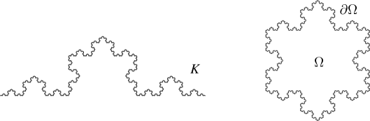
Figure 1: The Koch curve $K$ and Koch snowflake domain $\Omega$.

The Koch curve is a self-similar fractal with dimension $D:=\log_{3}4$ (Hausdorff and Minkowski dimensions coincide for the Koch curve) and may be constructed by means of its self-similar structure (as in [Ki, p. 15] or [Fa, Chap. 9]) as follows: let $\varrho=\tfrac{1}{2}+\tfrac{1}{2\sqrt{3}}i,$ with $i=\sqrt{-1}$, and define two maps on $\mathbb{C}$ by

$$f_{1}(z):=\varrho\overline{z}\quad\text{and}\quad f_{2}(z):=(1-\varrho)(\overline{z}-1)+1.$$

Then the Koch curve is the self-similar set of $\mathbb{R}^{2}$ with respect to $\{f_{1},f_{2}\}$; i.e., the unique nonempty compact set $K\subseteq\mathbb{R}^{2}$ satisfying $K=f_{1}(K)\cup f_{2}(K).$

In this paper, we prove the following new result:

Theorem 1.1

The area of the inner $\varepsilon$-neighbourhood of the Koch snowflake is given by the following tube formula:

$$V(\varepsilon)=G_{1}(\varepsilon)\varepsilon^{2-D}+G_{2}(\varepsilon)\varepsilon^{2},$$ (1.9)

where $D=\log_{3}4$ is the Minkowski dimension of $\partial$$\Omega$, ${\bf p}:=2\pi/\log 3$ is the oscillatory period, and $G_{1}$ and $G_{2}$ are periodic functions (of multiplicative period 3) which are discussed in full detail in Thm. 5.1. This formula may also be written

$$V(\varepsilon)=\sum_{n\in\mathbb{Z}}\varphi_{n}\varepsilon^{2-D-in{\bf p}}+\sum_{n\in\mathbb{Z}}\psi_{n}\varepsilon^{2-in{\bf p}},$$ (1.10)

for suitable constants $\varphi_{n},\psi_{n}$ which depend only on $n$. These constants are expressed in terms of the Fourier coefficients $g_{\alpha}$ of a multiplicative function which bears structural similarities to the classical Cantor–Lebesgue function described in more detail in §6.

While this formula is new, it should be noted that a previous approximation has been obtained in [La-vF1, §10.3]; see (2.10) in Rem. 2.5 below. Our present formula, however, is exact. By reading off the powers of $\varepsilon$ appearing in (1.10), we immediately obtain the following corollary:

Corollary 1.2

The possible complex dimensions of the Koch snowflake are

$$\mathcal{D}_{\partial\Omega}=\{D+in{\bf p}\rule{0.86108pt}{0.0pt}:\rule{0.86108pt}{0.0pt}n\in\mathbb{Z}\}\cup\{in{\bf p}\rule{0.86108pt}{0.0pt}:\rule{0.86108pt}{0.0pt}n\in\mathbb{Z}\}.$$ (1.11)

This is illustrated in Fig. 8. Also, for more precision regarding Cor. 1.2, see Rem. 5.3 below, as well as the discussion surrounding (5.5).

Remark 1.3

The significance of the tube formula (1.9) is that it gives a detailed account of the oscillations that are intrinsic to the geometry of the Koch snowflake curve. More precisely, the real part $D$ yields the order of the amplitude of these oscillations (as a function of $\varepsilon$) while the imaginary part $n{\bf p}=2\pi n/\log 3$ $(n=0,1,2,\dots)$ gives their frequencies. This is in agreement with the ‘philosophy’ of the mathematical theory of the complex dimensions of fractal strings as developed in [La-vF1]. Additionally, if one can show the existence of a complex dimension with real part $D$ and imaginary part $in{\bf p},n\neq 0$, then Theorem 1.1 immediately implies that the Koch curve is not Minkowski measurable, as conjectured in [La3, Conj. 2&3, pp. 159,163–4].

The rest of this paper is dedicated to the proof of Thm. 1.1 (stated more precisely as Thm. 5.1). More specifically, in §2 we approximate the area $V(\varepsilon)$ of the inner $\varepsilon$-neighborhood. In §3 we take into account the ‘error’ resulting from this approximation. We study the form of this error in §3.1, and the amount of it in §3.2. In §4 we combine §2 and §3 to deduce the tube formula (1.9) in the more precise form given in §5. We also include in §5 some comments on the interpretation of Thm. 5.1. Finally, in §6 we sketch the graph and briefly discuss some of the properties of the Cantor-like and multiplicatively periodic function $h(\varepsilon)$, the Fourier coefficients of which occur explicitly in the expansion of $V(\varepsilon)$ stated in Thm. 5.1.

Acknowledgements. The authors are grateful to Machiel van Frankenhuysen for his comments on a preliminary version of this paper. In particular, for indicating the current, more elegant and concise presentation of the main result (5.1). We also wish to thank Victor Shapiro for a helpful discussion concerning Fourier series, especially with regard to the discussion surrounding (4.8).

2 Estimating the area

Figure 2: The first four stages in the geometric construction of $K$.

Consider an approximation to the inner $\varepsilon$-neighbourhood of the Koch curve, as shown in Fig. 3. Although we will eventually compute the neighborhood for the entire snowflake, we work with one third of it throughout the sequel (as depicted in the figure).

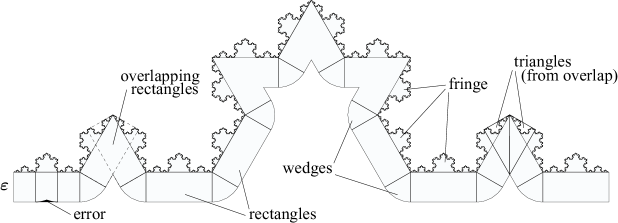
Figure 3: An approximation to the inner $\varepsilon$-neighbourhood of the Koch curve, with $\varepsilon\in I_{2}$. The refinement level here is based on the graph $K_{2}$, the second stage in the geometric construction of the Koch curve (see Fig. 2).

We will determine the area of the $\varepsilon$-neighbourhood with functions that give the area of each kind of piece (rectangle, wedge, fringe, as shown in the figure) in terms of $\varepsilon$, and functions that count the number of each of these pieces, in terms of $\varepsilon$. As seen by comparing Fig. 3 to Fig. 4, the number of such pieces increases exponentially.

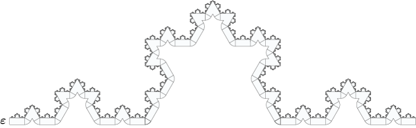
Figure 4: A smaller $\varepsilon$-neighbourhood of the Koch curve, for $\varepsilon\in I_{3}$. This refinement level is based on the graph $K_{3}$, the third stage in the construction of the Koch curve.

We take the base of the Koch curve to have length 1, and carry out our approximation for different values of $\varepsilon$, as $\varepsilon\to 0^{+}$. In particular, let

$$I_{n}:=(3^{-(n+1)}/\sqrt{3},3^{-n}/\sqrt{3}].$$ (2.1)

Whenever $\varepsilon=3^{-n}/\sqrt{3}$, the approximation shifts to the next level of refinement. For example, Fig. 3 shows $\varepsilon\in I_{2}$, and Fig. 4 shows $\varepsilon\in I_{3}$. Consequently, for $\varepsilon\in I_{0}$, it suffices to consider an $\varepsilon$-neighbourhood of the prefractal curve $K_{0}$ , and for $\varepsilon\in I_{1}$, it suffices to consider an $\varepsilon$-neighbourhood of the prefractal curve $K_{1}$, etc. Fig. 2 shows these prefractal approximations.

In general, we will discuss a neighbourhood of $K_{n}$, and we define the function

$$n=n(\varepsilon):=\left[\log_{3}\frac{1}{\varepsilon\sqrt{3}}\right]=\left[x\right]$$ (2.2)

to tell us for what $n$ we have $\varepsilon\in I_{n}$. Here, the square brackets indicate the floor function (integer part) and

$$x:=-\log_{3}(\varepsilon\sqrt{3}),$$ (2.3)

a notation which will frequently prove convenient in the sequel. Further, we let

$$\{x\}:=x-[x]\in[0,1)$$ (2.4)

denote the fractional part of $x$.

Observe that for $\varepsilon\in I_{n}$, $n$ is fixed even as $\varepsilon$ is changing. To see how this is useful, consider that for all $\varepsilon$ in this interval, the number of rectangles (including those which overlap in the corners) is readily seen to be the fixed number

$$r_{n}:=4^{n}.$$ (2.5)

Also, each of these rectangles has area $\varepsilon 3^{-n}$, where $n$ is fixed as $\varepsilon$ traverses $I_{n}$. Continuing in this constructive manner, we prove the following lemma.

Lemma 2.1

For $\varepsilon\in I_{n}$, there are

• $r_{n}=4^{n}$ rectangles, each with area $\varepsilon 3^{-n}$,

• $w_{n}=\frac{2}{3}(4^{n}-1)$ wedges, each with area $\frac{\pi\varepsilon^{2}}{6}$,

• $u_{n}=\frac{2}{3}(4^{n}+2)$ triangles, each with area $\frac{\varepsilon^{2}\sqrt{3}}{2}$, and

• $4^{n}$ components of fringe, each with area $\frac{\sqrt{3}}{20}9^{-n}$.

Proof 2.2.

We have already established (i).

For (ii), we exploit the self-similarity of the Koch curve $K$ to obtain the recurrence relation $w_{n}=4w_{n-1}+2$, which we solve to find the number of wedges

$$w_{n}:=\sum_{j=0}^{n-1}{2\cdot 4^{j}}=\tfrac{2}{3}\left(4^{n}-1\right).$$ (2.6)

The area of each wedge is clearly $\pi\varepsilon^{2}/6,$ as the angle is always fixed at $\pi/3$.

(iii) To prevent double-counting, we will need to keep track of the number of rectangles that overlap in the acute angles so that we may subtract the appropriate number of triangles

$$u_{n}:=4^{n}-\sum_{j=1}^{n-1}4^{j}=\tfrac{2}{3}\left(4^{n}+2\right).$$ (2.7)

Each of these triangles has area $\varepsilon^{2}\sqrt{3}/2$.

(iv) To measure the area of the fringe, note that the area under the entire Koch curve is given by $\sqrt{3}/20$, so the fringe of $K_{n}$ will be this number scaled by $\left(3^{-n}\right)^{2}$. There are $4^{n}$ components, one atop each rectangle (see Fig. 3).

Lemma 2.1 gives a preliminary area formula for the $\varepsilon$-neighbourhood. Here, ‘preliminary’ indicates the absence of the ‘error estimate’ developed in §3.

Lemma 2.3.

The $\varepsilon$-neighbourhood of the Koch curve has approximate area

$$\widetilde{V}(\varepsilon)=\varepsilon^{2-D}4^{-\{x\}}\left(\tfrac{3\sqrt{3}}{40}9^{\{x\}}+\tfrac{\sqrt{3}}{2}3^{\{x\}}+\tfrac{1}{6}\left(\tfrac{\pi}{3}-\sqrt{3}\right)\right)-\tfrac{\varepsilon^{2}}{3}\left(\tfrac{\pi}{3}+2\sqrt{3}\right).$$ (2.8)

This formula is approximate in the sense that it measures a region slightly larger than the actual $\varepsilon$-neighbourhood. This discrepancy is accounted for and analyzed in detail in §3.

Proof 2.4 (of Lemma 2.3).

Using (2.2) and (2.3), we obtain:

$$4^{x}=\tfrac{1}{2}\varepsilon^{-D},\rule{12.91663pt}{0.0pt}9^{-x}=3\varepsilon^{2},\rule{12.91663pt}{0.0pt}\left(\tfrac{4}{3}\right)^{x}=\tfrac{\sqrt{3}}{2}\varepsilon^{1-D},\rule{12.91663pt}{0.0pt}\left(\tfrac{4}{9}\right)^{x}=\tfrac{3}{2}\varepsilon^{2-D}.$$ (2.9)

Now using $n=[x]=x-\{x\}$, we compute the contributions of the rectangles, wedges, triangles, and fringe, respectively, as

$$\widetilde{V}_{r}(\varepsilon) =\varepsilon\left(\tfrac{4}{3}\right)^{n}=\varepsilon^{2-D}\tfrac{\sqrt{3}}{2}\cdot 4^{-\{x\}}3^{\{x\}},$$

$$\widetilde{V}_{w}(\varepsilon) =\tfrac{\pi\varepsilon^{2}}{9}(4^{n}-1)=\varepsilon^{2-D}\tfrac{\pi}{18}\cdot 4^{-\{x\}}-\varepsilon^{2}\tfrac{\pi}{9},$$

$$\widetilde{V}_{u}(\varepsilon) =\tfrac{\varepsilon^{2}\sqrt{3}}{3}\left(4^{n}+2\right)=\varepsilon^{2-D}\tfrac{\sqrt{3}}{6}\cdot 4^{-\{x\}}+\varepsilon^{2}\tfrac{2\sqrt{3}}{3},\text{ and}$$

$$\widetilde{V}_{\text{f}}(\varepsilon) =\left(\tfrac{4}{9}\right)^{n}\left(\tfrac{\sqrt{3}}{20}\right)=\varepsilon^{2-D}\tfrac{3\sqrt{3}}{40}\cdot 4^{-\{x\}}9^{\{x\}}.$$

Putting all this together, $\widetilde{V}=\widetilde{V}_{r}+\widetilde{V}_{w}-\widetilde{V}_{u}+\widetilde{V}_{\text{f}}$ gives the result.

Remark 2.5.

It is pleasing to find that this is in agreement with earlier predictions of what $\widetilde{V}(\varepsilon)$ should look like. In particular, [La-vF1, p. 209] gives the estimate

$$V(\varepsilon)\approx\varepsilon^{2-D}\frac{\sqrt{3}}{4}4^{-\{x\}}\left(\frac{3}{5}9^{\{x\}}+6\cdot 3^{\{x\}}-1\right),$$ (2.10)

which differs only from our formula for $\widetilde{V}(\varepsilon)$ in (2.8) by some constants and the final term of order $\varepsilon^{2}$.

In (3.9) we will require the Fourier series of the periodic function $\varepsilon^{-(2-D)}\widetilde{V}(\varepsilon)$ as it is given by (2.8), so we recall the formula

$$a^{-\{x\}}=\frac{a-1}{a}\sum_{n\in\mathbb{Z}}\frac{e^{2\pi inx}}{\log a+2\pi in}.$$ (2.11)

This formula is valid for $a>0,a\neq 1$ and has been used repeatedly in [La-vF1]. Note that it follows from Dirichlet’s Theorem and thus holds in the sense of Fourier series. In particular, the series in (2.11) converges pointwise; this is also true in (2.13) and (2.14) below.

We will make frequent use of the following identity in the sequel:

$$e^{2\pi inx}=\left(\varepsilon\sqrt{3}\right)^{-in{\bf p}}=(-1)^{n}\varepsilon^{-in{\bf p}},\quad\text{ for }n\in\mathbb{Z},$$ (2.12)

where ${\bf p}=2\pi/\log 3$ is the oscillatory period as in Thm. 1.1. With $x=-\log_{3}(\varepsilon\sqrt{3})$, we can rewrite the Fourier expansion of $a^{-\{x\}}$ given in (2.11) as

$$a^{-\{x\}}=\frac{a-1}{a\log 3}\sum_{n\in\mathbb{Z}}\frac{(-1)^{n}\varepsilon^{-in{\bf p}}}{\log_{3}a+in{\bf p}}.$$ (2.13)

Recall that $\{x\}=x-[x]$ denotes the fractional part of $x$. With $D=\log_{3}4$, we use (2.13) to express (2.8) as a pointwise convergent Fourier series in $\varepsilon$:

$$\widetilde{V}(\varepsilon) =\tfrac{1}{3\log 3}\sum_{n\in\mathbb{Z}}\left(\tfrac{-3^{5/2}}{2^{5}(D-2+in{\bf p})}+\tfrac{3^{3/2}}{2^{3}(D-1+in{\bf p})}+\tfrac{\pi-3^{3/2}}{2^{3}(D+in{\bf p})}\right)(-1)^{n}\varepsilon^{2-D-in{\bf p}}$$

$$\rule{215.2771pt}{0.0pt}-\tfrac{1}{3}\left(\tfrac{\pi}{3}+2\sqrt{3}\right)\varepsilon^{2}.$$ (2.14)

3 Computing the error

Now we must account for all the little ‘trianglets’, the small regions shaped like a crest of water on an ocean wave. These regions were included in our original calculation, but now must be subtracted. This error appeared in each of the rectangles counted earlier, and so we refer to all the error from one of these rectangles as an ‘error block’. Fig. 5 shows how this error is incurred and how it inherits a Cantoresque structure from the Koch curve.

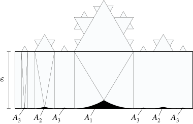
Figure 5: An error block for $\varepsilon\in I_{n}$. The central third of the block contains one large isosceles triangle, two wedges, and the trianglet $A_{1}$.

Actually, we will see in §3.2 that this ‘error’ will have several terms, some of which are of the same order as the leading term in $\widetilde{V}(\varepsilon)$, which is proportional to $\varepsilon^{2-D}$ by (2.14). Hence, caution should be exercised when carrying out such computations and one should not be too quick to set aside terms that appear negligible.

3.1 Finding the area of an ‘error block’

In calculating the error, we begin by finding the area of one of these error blocks. Later, we will count how many of these error blocks there are, as a function of $\varepsilon$. Note that $n$ is fixed throughout §3.1, but $\varepsilon$ varies within $I_{n}$. We define the function

$$w=w(\varepsilon):=3^{-n}=3^{-[x]}.$$ (3.1)

This function $w(\varepsilon)$ gives the width of one of the rectangles, as a function of $\varepsilon$ (see Fig. 6). Note that $w(\varepsilon)$ is constant as $\varepsilon$ traverses $I_{n}$, as is $n=n(\varepsilon)$. From Fig. 6, one can work out that the area of both wedges adjacent to $A_{k}$ is

$$\varepsilon^{2}\sin^{-1}\left(\tfrac{w}{2\cdot 3^{k}\varepsilon}\right),$$

and that the area of the triangle above $A_{k}$ is

$$\varepsilon\tfrac{w}{2\cdot 3^{k}}\sqrt{1-\left(\tfrac{w}{2\cdot 3^{k}\varepsilon}\right)^{2}}.$$

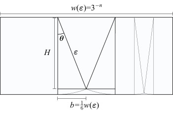
Figure 6: Finding the height of the central triangle.

Then for $k=1,2,\dots,$ the area of the trianglet $A_{k}$ is given by

$$A_{k}(\varepsilon)=\varepsilon\frac{w(\varepsilon)}{3^{k}}-\varepsilon^{2}\sin^{-1}\left(\frac{w(\varepsilon)}{2\cdot 3^{k}\varepsilon}\right)-\varepsilon\frac{w(\varepsilon)}{2\cdot 3^{k}}\sqrt{1-\left(\frac{w(\varepsilon)}{2\cdot 3^{k}\varepsilon}\right)^{2}},$$ (3.2)

and appears with multiplicity $2^{k-1}$, as in Fig. 5. We use (3.1) and (2.3) to write $w(\varepsilon)=3^{-x}3^{\{x\}}=\varepsilon\sqrt{3}(\tfrac{1}{3})^{-\{x\}},$ and define

$$3^{x}_{k}:=\tfrac{w}{3^{k}\varepsilon}=3^{\{x\}-k+1/2}.$$ (3.3)

Hence the entire contribution of one error block may be written as

$$B(\varepsilon): =\sum_{k=1}^{\infty}2^{k-1}\left(3^{x}_{k}-\sin^{-1}\left(\tfrac{3^{x}_{k}}{2}\right)-\tfrac{3^{x}_{k}}{2}\sqrt{1-\left(\tfrac{3^{x}_{k}}{2}\right)^{2}}\right)\varepsilon^{2}.$$ (3.4)

Recall the power series expansions

$$\sin^{-1}u=\sum_{m=0}^{\infty}{\tfrac{(2m)!\,u^{2m+1}}{2^{2m}(m!)^{2}(2m+1)}}\quad\text{ and }\quad\sqrt{1-u^{2}}=1-\sum_{m=0}^{\infty}{\tfrac{(2m)!\,u^{2m+2}}{2^{2m+1}m!(m+1)!}},$$

which are valid for $|u|<1$. We use these formulae with $u=\frac{w}{2\cdot 3^{k}\varepsilon}$, so convergence is guaranteed by

$$0\leq\tfrac{w}{2\cdot 3^{k}\varepsilon}=\tfrac{3^{\{x\}}\sqrt{3}}{2\cdot 3^{k}}\leq\tfrac{\sqrt{3}}{2}<1,$$

and the fact that the series in (3.4) starts with $k=1$. Then (3.4) becomes

$$B(\varepsilon) =\sum_{k=1}^{\infty}2^{k-1}\left[\tfrac{3^{x}_{k}}{2}+\sum_{m=0}^{\infty}\tfrac{(2m)!\,(3^{x}_{k})^{2m+3}}{2^{4m+4}m!(m+1)!}-\sum_{m=0}^{\infty}\tfrac{(2m)!\,(3^{x}_{k})^{2m+1}}{2^{4m+1}(m!)^{2}(2m+1)}\right]\varepsilon^{2}$$

$$=\sum_{k=1}^{\infty}2^{k-1}\left[\sum_{m=1}^{\infty}\tfrac{(2m-2)!\,(3^{x}_{k})^{2m+1}}{2^{4m}(m-1)!m!}-\sum_{m=1}^{\infty}\tfrac{(2m)!\,(3^{x}_{k})^{2m+1}}{2^{4m+1}(m!)^{2}(2m+1)}\right]\varepsilon^{2}$$

$$=\sum_{m=1}^{\infty}\sum_{k=1}^{\infty}\tfrac{2^{k-1}}{(3^{2m+1})^{k}}\tfrac{(2m-2)!\,(3^{\{x\}+1/2})^{2m+1}}{2^{4m}(m-1)!m!}\left(1-\tfrac{(2m-1)2m}{2m(2m+1)}\right)\varepsilon^{2}$$

$$=\sum_{m=1}^{\infty}\tfrac{1}{3^{2m+1}}\left(\tfrac{1}{(3^{2m+1}-2)/3^{2m+1}}\right)\tfrac{(2m-2)!\,(\sqrt{3})^{2m+1}}{2^{4m-1}(m-1)!m!(2m+1)}\left(\tfrac{1}{3^{2m+1}}\right)^{-\{x\}}\varepsilon^{2}$$

$$=\sum_{m=1}^{\infty}\tfrac{(2m-2)!}{2^{4m-1}(m-1)!m!(2m+1)(3^{2m+1}-2)}\left(\tfrac{1}{3^{2m+1}}\right)^{-\{x\}}\varepsilon^{2}.$$ (3.5)

The interchange of sums is validated by checking absolute convergence of the final series via the ratio test, and then applying Fubini’s Theorem to retrace our steps.

3.2 Counting the error blocks

Some blocks are present in their entirety as $\varepsilon$ traverses an interval $I_{n}$, while others are in the process of forming: two in each of the peaks and one at each end (see Fig. 7). Using the same notation as previously in Lemma 2.1, we count the complete and partial error blocks with

$$c_{n} =r_{n}-u_{n}=\tfrac{1}{3}\left(4^{n}-4\right),\quad\text{and}\quad p_{n}=u_{n}=\tfrac{2}{3}\left(4^{n}+2\right).$$

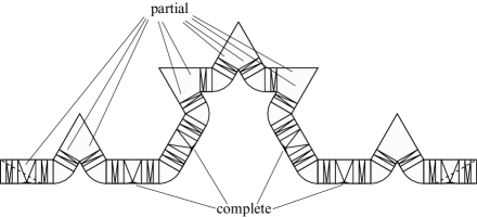
Figure 7: Error block formation. The ends are counted as partial because three of these pieces will be added together to make the entire snowflake.

By means of (2.2)–(2.4), we convert $c_{n}$ and $p_{n}$ into functions of the continuous variable $\varepsilon$, where $\varepsilon>0$:

$$c(\varepsilon) =\tfrac{1}{3}\left(\tfrac{\varepsilon^{-D}}{2}4^{-\{x\}}-4\right)\quad\text{ and }\quad p(\varepsilon)=\tfrac{2}{3}\left(\tfrac{\varepsilon^{-D}}{2}4^{-\{x\}}+2\right).$$ (3.6)

With $B(\varepsilon)$ given by (3.1), the total error is thus

$$E(\varepsilon)=B(\varepsilon)\left[c(\varepsilon)+p(\varepsilon)h(\varepsilon)\right].$$ (3.7)

Remark 3.1.

The function $h(\varepsilon)$ in (3.7) is some periodic function that oscillates multiplicatively in a region bounded between 0 and 1, indicating what portion of the partial error block has formed; see Fig. 5 and Fig. 7. We do not know $h(\varepsilon)$ explicitly, but we do know by the self-similarity of $K$ that it has multiplicative period 3; i.e., $h(\varepsilon)=h(\tfrac{\varepsilon}{3})$. Using (2.12), the Fourier expansion

$$h(\varepsilon)=\sum_{\alpha\in\mathbb{Z}}g_{\alpha}(-1)^{\alpha}\varepsilon^{-i\alpha{\bf p}}=\sum_{\alpha\in\mathbb{Z}}g_{\alpha}e^{2\pi i\alpha x}=g(x)$$ (3.8)

shows that we may also consider $h(\varepsilon)$ as an additively periodic function of the variable $x=-\log_{3}(\varepsilon\sqrt{3})$, with additive period 1. We refer the interested reader to §6 below for a further discussion of $h(\varepsilon)$, including a sketch of its graph, justification of the convergence of (3.8), and a brief discussion of some of its properties.

We now return to the computation; substituting (3.1) and (3.6) into (3.7) gives

$$E(\varepsilon) =B(\varepsilon)\left[\tfrac{\varepsilon^{-D}}{3}4^{-\{x\}}\left(\tfrac{1}{2}+h(\varepsilon)\right)+\tfrac{4}{3}\left(h(\varepsilon)-1\right)\right]$$

$$=\tfrac{1}{3}\sum_{m=1}^{\infty}\tfrac{(2m-2)!(h(\varepsilon)+1/2)}{2^{4m-1}(m-1)!m!(2m+1)(3^{2m+1}-2)}\left(\tfrac{4}{3^{2m+1}}\right)^{-\{x\}}\varepsilon^{2-D}$$

$$\rule{55.97205pt}{0.0pt}+\tfrac{1}{3}\sum_{m=1}^{\infty}\tfrac{(2m-2)!(h(\varepsilon)-1)}{2^{4m-3}(m-1)!m!(2m+1)(3^{2m+1}-2)}\left(\tfrac{1}{3^{2m+1}}\right)^{-\{x\}}\varepsilon^{2}$$

$$=\tfrac{1}{3\log 3}\sum_{m=1}^{\infty}\sum_{n\in\mathbb{Z}}\tfrac{(2m-2)!(4-3^{2m+1})(-1)^{n}(h(\varepsilon)+1/2)}{2^{4m+1}(m-1)!m!(2m+1)(3^{2m+1}-2)(D-2m-1+in{\bf p})}\varepsilon^{2-D-in{\bf p}}$$

$$\rule{55.97205pt}{0.0pt}+\tfrac{1}{3\log 3}\sum_{m=1}^{\infty}\sum_{n\in\mathbb{Z}}\tfrac{(2m-2)!(1-3^{2m+1})(-1)^{n}(h(\varepsilon)-1)}{2^{4m-3}(m-1)!m!(2m+1)(3^{2m+1}-2)(-2m-1+in{\bf p})}\varepsilon^{2-in{\bf p}}$$

$$=\tfrac{1}{3\log 3}\sum_{n\in\mathbb{Z}}(h(\varepsilon)+1/2)(-b_{n})(-1)^{n}\varepsilon^{2-D-in{\bf p}}$$

$$\rule{55.97205pt}{0.0pt}+\tfrac{1}{3\log 3}\sum_{n\in\mathbb{Z}}(h(\varepsilon)-1)(-\tau_{n})(-1)^{n}\varepsilon^{2-in{\bf p}},$$ (3.9)

where we have written the constants $b_{n}$ and $\tau_{n}$ in the shorthand notation as follows:

$$b_{n} :=\sum_{m=1}^{\infty}\tfrac{(2m-2)!(3^{2m+1}-4)}{2^{4m+1}(m-1)!m!(2m+1)(3^{2m+1}-2)(D-2m-1+in{\bf p})},$$ (3.10)

$$\text{ and }\tau_{n} :=\sum_{m=1}^{\infty}\tfrac{(2m-2)!(3^{2m+1}-1)}{2^{4m-3}(m-1)!m!(2m+1)(3^{2m+1}-2)(-2m-1+in{\bf p})}.$$ (3.11)

In the third equality of (3.9), we have applied (2.13) to $a=4/3^{2m+1}$ and to $a=1/3^{2m+1}$, respectively. By the ratio test, the complex numbers $b_{n}$ and $\tau_{n}$ given by (3.10) and (3.11) are well-defined. This fact, combined with Fubini’s Theorem, enables us to justify the interchange of sums in the last equality of (3.9).

4 Computing the area

Now that we have estimate (2.14) for the area of the neighbourhood of the Koch curve $\widetilde{V}(\varepsilon)$, and formula (3.9) for the ‘error’ $E(\varepsilon)$, we can find the exact area of the inner neighbourhood of the full Koch snowflake as follows:

$$V(\varepsilon) =3\left(\widetilde{V}(\varepsilon)-E(\varepsilon)\right)$$

$$=\tfrac{1}{\log 3}\sum_{n\in\mathbb{Z}}\left(\tfrac{-3^{5/2}}{2^{5}(D-2+in{\bf p})}+\tfrac{3^{3/2}}{2^{3}(D-1+in{\bf p})}+\tfrac{\pi-3^{3/2}}{2^{3}(D+in{\bf p})}\right)(-1)^{n}\varepsilon^{2-D-in{\bf p}}$$

$$\rule{21.52771pt}{0.0pt}+\tfrac{1}{\log 3}\sum_{n\in\mathbb{Z}}(h(\varepsilon)+1/2)(-1)^{n}b_{n}\varepsilon^{2-D-in{\bf p}}$$

$$\rule{21.52771pt}{0.0pt}-\left(\tfrac{\pi}{3}+2\sqrt{3}\right)\varepsilon^{2}+\tfrac{1}{\log 3}\sum_{n\in\mathbb{Z}}(h(\varepsilon)-1)(-1)^{n}\tau_{n}\varepsilon^{2-in{\bf p}}$$

$$=\tfrac{1}{\log 3}\sum_{n\in\mathbb{Z}}\left(\tfrac{-3^{5/2}}{2^{5}(D-2+in{\bf p})}+\tfrac{3^{3/2}}{2^{3}(D-1+in{\bf p})}+\tfrac{\pi-3^{3/2}}{2^{3}(D+in{\bf p})}\right.$$

$$\rule{154.99951pt}{0.0pt}\left.\rule{0.0pt}{9.47217pt}+\tfrac{b_{n}}{2}+h(\varepsilon)b_{n}\right)(-1)^{n}\varepsilon^{2-D-in{\bf p}}$$

$$\rule{21.52771pt}{0.0pt}+\tfrac{1}{\log 3}\sum_{n\in\mathbb{Z}}\left(-\tau_{n}-\log 3\left(\tfrac{\pi}{3}+2\sqrt{3}\right)\delta_{0}^{n}+h(\varepsilon)\tau_{n}\right)(-1)^{n}\varepsilon^{2-in{\bf p}},$$ (4.1)

where $\delta_{0}^{n}$ is the Kronecker delta. Therefore, we have

$$V(\varepsilon)=G_{1}(\varepsilon)\varepsilon^{2-D}+G_{2}(\varepsilon)\varepsilon^{2},$$ (4.2)

where the periodic functions $G_{1}$ and $G_{2}$ are given by

$$G_{1}(\varepsilon): =\frac{1}{\log 3}\sum_{n\in\mathbb{Z}}\left(a_{n}+b_{n}h(\varepsilon)\right)(-1)^{n}\varepsilon^{-in{\bf p}}$$ (4.3)

$$\text{ and \;}G_{2}(\varepsilon): =\frac{1}{\log 3}\sum_{n\in\mathbb{Z}}\left(\sigma_{n}+\tau_{n}h(\varepsilon)\right)(-1)^{n}\varepsilon^{-in{\bf p}}.$$ (4.4)

Here we have used (3.10) and (3.11), and introduced the notation $a_{n}$ and $\sigma_{n}$ (stated explicitly in (5.3)). We wish to rearrange these series so as to collect all factors of $\varepsilon$. First, we can split the sum in (4.3) as

$$G_{1}(\varepsilon) =\frac{1}{\log 3}\sum_{n\in\mathbb{Z}}a_{n}(-1)^{n}\varepsilon^{-in{\bf p}}+\frac{h(\varepsilon)}{\log 3}\sum_{n\in\mathbb{Z}}b_{n}(-1)^{n}\varepsilon^{-in{\bf p}}$$ (4.5)

because $a(\varepsilon):=\sum_{n\in\mathbb{Z}}a_{n}(-1)^{n}\varepsilon^{-in{\bf p}}$ and $b(\varepsilon):=\sum_{n\in\mathbb{Z}}b_{n}(-1)^{n}\varepsilon^{-in{\bf p}}$ are each convergent: $a(\varepsilon)$ converges for the same reason as (2.14), and one can show that

$$b(\varepsilon)=\sum_{m=0}^{\infty}\tfrac{(4\log 3)(2m-2)!}{2^{4m+1}3^{m-1/2}(m-1)!m!(2m+1)(3^{2m+1}-2)}\left(\tfrac{4}{3^{2m+1}}\right)^{-\{x\}}$$ (4.6)

converges to a well-defined distribution induced by a locally integrable function; one proves directly that $|b_{n}|\leq c/|n|$ by writing (3.10) as

$$b_{n} =\sum_{m=1}^{\infty}\tfrac{\beta_{m}}{D-2m-1+in{\bf p}},\quad\text{ with }\quad\sum_{m=1}^{\infty}\beta_{m}\,<\,\infty.$$ (4.7)

Then the rearrangement leading to (4.6) is justified via the “descent method” with $q=2$, as described in Rem. 4.1 below. Note that the right-hand side of (4.6) converges by the ratio test and is thus defined pointwise on $\mathbb{R}\sim\mathbb{Z}$. Therefore one also sees that $b(\varepsilon)$ and $h(\varepsilon)$ are periodic functions. Considered as functions of the variable $x=\log_{3}(1/\varepsilon\sqrt{3})$, both have period 1 with $b$ continuous for $0\leq x<1$ and $h$ continuous for $0<x\leq 1$. Further, each is monotonic on its period interval, and possesses a bounded jump discontinuity only at the endpoint. This may be seen for $b(\varepsilon)$ from (4.6) and for $h(\varepsilon)$ from §6.

Although we have used distributional arguments to obtain (4.6), the right-hand side of (4.6) is locally integrable and has a representation as a piecewise continuous function. Thus the distributional equality in (4.6) actually holds pointwise in the sense of Fourier series and all our results are still valid pointwise. Recall that the Dirichlet–Jordan Theorem [Zy, Thm. II.8.1] states that if $f$ is periodic and (locally) of bounded variation, its Fourier series converges pointwise to $\left(f(x-)+\rule{0.0pt}{8.61108pt}f(x+)\right)/2$. As described above, $b(\varepsilon)$ and $h(\varepsilon)$ are each of bounded variation and therefore by [Zy, Thm. II.4.12] we have $b_{n}=O(1/n)\text{ and }g_{n}=O(1/n)\text{ as }n\to\pm\infty.$ Finally, [Zy, Thm. IX.4.11] may be applied to yield the pointwise equality

$$b(\varepsilon)h(\varepsilon)=\sum_{n\in\mathbb{Z}}\sum_{\alpha\in\mathbb{Z}}b_{\alpha}g_{n-\alpha}(-1)^{n}\varepsilon^{-in{\bf p}}.$$ (4.8)

This theorem applies because (4.6) shows that $b(\varepsilon)$ is bounded away from 0.

Now that all the $\varepsilon$’s are combined, we substitute (4.8) back into (4.5) and rewrite $G_{1}(\varepsilon)=\left(a(\varepsilon)+\rule{0.0pt}{8.61108pt}b(\varepsilon)h(\varepsilon)\right)/\log 3$ as in (5.2a):

$$G_{1}(\varepsilon) =\frac{1}{\log 3}\sum_{n\in\mathbb{Z}}\left(a_{n}+\sum_{\alpha\in\mathbb{Z}}b_{\alpha}g_{n-\alpha}\right)(-1)^{n}\varepsilon^{-in{\bf p}}.$$ (4.9)

Manipulating $G_{2}(\varepsilon)$ similarly, we are able to rewrite (4.4) in its final form (5.2b), and thereby complete the proof of Thm. 5.1.

Remark 4.1.

The convergence of the Fourier series associated to a periodic distribution is proved via the descent method by integrating both sides $q$ times (for sufficiently large $q$) so that one has pointwise convergence. After enough integrations, the distribution will be a smooth function, the series involved will converge absolutely, and the Weierstrass theorem can be applied pointwise. At this point, rearrangements or interchanges of series are justified pointwise, and we obtain a pointwise formula for the $q^{\text{th}}$ antiderivative of the desired function. Then one takes the distributional derivative $q$ times to obtain the desired formula. See [La-vF1, Rem. 4.14]. How large the positive integer $q$ needs to be depends on the order of polynomial growth of the Fourier coefficients. Recall that the Fourier series of a periodic distribution converges distributionally if and only if the Fourier coefficients are of slow growth, i.e., do not grow faster than polynomially. Moreover, from the point of view of distributions, there is no distinction to be made between convergent trigonometric series and Fourier series. See [Sch, §VII,I].

5 Main results

We can now state our main result in the following more precise form of Thm. 1.1:

Theorem 5.1.

The area of the inner $\varepsilon$-neighbourhood of the Koch snowflake is given pointwise by the following tube formula:

$$V(\varepsilon)=G_{1}(\varepsilon)\varepsilon^{2-D}+G_{2}(\varepsilon)\varepsilon^{2},$$ (5.1)

where $G_{1}$ and $G_{2}$ are periodic functions of multiplicative period 3, given by

$$G_{1}(\varepsilon): =\frac{1}{\log 3}\sum_{n\in\mathbb{Z}}\left(a_{n}+\sum_{\alpha\in\mathbb{Z}}b_{\alpha}g_{n-\alpha}\right)(-1)^{n}\varepsilon^{-in{\bf p}}$$ (5.2a)

$$\text{ and \;}G_{2}(\varepsilon): =\frac{1}{\log 3}\sum_{n\in\mathbb{Z}}\left(\sigma_{n}+\sum_{\alpha\in\mathbb{Z}}\tau_{\alpha}g_{n-\alpha}\right)(-1)^{n}\varepsilon^{-in{\bf p}},$$ (5.2b)

where $a_{n},b_{n},\sigma_{n},$ and $\tau_{n}$ are the complex numbers given by

$$a_{n} =-\frac{3^{5/2}}{2^{5}(D-2+in{\bf p})}+\frac{3^{3/2}}{2^{3}(D-1+in{\bf p})}+\frac{\pi-3^{3/2}}{2^{3}(D+in{\bf p})}+\frac{1}{2}b_{n},$$

$$b_{n} =\sum_{m=1}^{\infty}\frac{(2m)!\;(3^{2m+1}-4)}{4^{2m+1}(m!)^{2}(4m^{2}-1)(3^{2m+1}-2)(D-2m-1+in{\bf p})},$$

$$\sigma_{n} =-\log 3\left(\frac{\pi}{3}+2\sqrt{3}\right)\delta_{0}^{n}-\tau_{n},\text{ and }$$ (5.3)

$$\tau_{n} =\sum_{m=1}^{\infty}\frac{(2m)!\;(3^{2m+1}-1)}{4^{2m-1}(m!)^{2}(4m^{2}-1)(3^{2m+1}-2)(-2m-1+in{\bf p})},$$

where $\delta_{0}^{\,0}=1$ and $\delta_{0}^{n}=0$ for $n\neq 0$ is the Kronecker delta.

In Thm. 5.1, $D=\log_{3}4$ is the Minkowski dimension of the Koch snowflake $\partial$$\Omega$ and ${\bf p}=2\pi/\log 3$ is its oscillatory period, following the terminology of [La-vF1]. The numbers $g_{\alpha}$ appearing in (5.2) are the Fourier coefficients of the periodic function $h(\varepsilon)$, a suitable nonlinear analogue of the Cantor–Lebesgue function, defined in Rem. 3.1 and further discussed in §6 below.

The reader may easily check that formula (5.1) can also be written

$$V(\varepsilon)=\sum_{n\in\mathbb{Z}}\varphi_{n}\varepsilon^{2-D-in{\bf p}}+\sum_{n\in\mathbb{Z}}\psi_{n}\varepsilon^{2-in{\bf p}},$$ (5.4)

for suitable constants $\varphi_{n},\psi_{n}$ which depend only on $n$. Now by analogy with the tube formula (1.8) from [La-vF1], we interpret the exponents of $\varepsilon$ in (5.4) as the ‘complex co-dimensions’ of $\partial$$\Omega$. Hence, we can simply read off the possible complex dimensions, and as depicted in Fig. 8, we obtain a set of possible complex dimensions

$$\mathcal{D}_{\partial\Omega}=\{D+in{\bf p}\rule{0.86108pt}{0.0pt}:\rule{0.86108pt}{0.0pt}n\in\mathbb{Z}\}\cup\{in{\bf p}\rule{0.86108pt}{0.0pt}:\rule{0.86108pt}{0.0pt}n\in\mathbb{Z}\}.$$ (5.5)

One caveat should be mentioned: this is assuming that none of the coefficients $\varphi_{n}$ or $\psi_{n}$ vanishes in (5.4). Indeed, in that case we would only be able to say that the complex dimensions are a subset of the right-hand side of (5.5). We expect that, following the ‘approximate tube formula’ obtained in [La-vF1], the set of complex dimensions should contain all numbers of the form $D+in{\bf p}$.

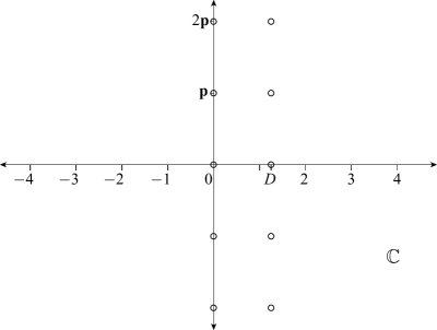
Figure 8: The possible complex dimensions of $K$ and $\partial\Omega$. The Minkowski dimension is $D=\log_{3}4$ and the oscillatory period is ${\bf p}=\tfrac{2\pi}{\log 3}$.

Remark 5.2.

We expect our methods to work for all lattice self-similar fractals (i.e., those for which the underlying scaling ratios are rationally dependent) as well as for other examples considered in [La-vF1] including the Cantor–Lebesgue curve, a self-affine fractal. For example, we have already obtained the counterpart of Thm. 5.1 for the square (rather than triangular) snowflake curve. By applying density arguments (as in [La-vF1, Chap. 2]), our methods may also yield information about the complex dimensions of nonlattice fractals.

Remark 5.3.

It should be pointed out that in the present paper, we do not provide a direct definition of the complex dimensions of the Koch snowflake curve $\partial$$\Omega$ (or of other fractals in $\mathbb{R}^{2}$). Instead, we reason by analogy with formula (1.8) above to deduce from our tube formula (5.1) the possible complex dimensions of $\partial$$\Omega$ (or of $K$). As is seen in the proof of Thm. 5.1, the tube formula for the Koch curve $K$ is of the same form as for that of the snowflake curve $\partial$$\Omega$. It follows that $K$ and $\partial$$\Omega$ have the same possible complex dimensions (see Cor. 1.2). In subsequent work, we plan to define the geometric zeta function $\zeta_{\partial\Omega}=\zeta_{\partial\Omega}(s)$ in this context to actually deduce the complex dimensions of $\partial$$\Omega$ directly as the poles of the meromorphic continuation of $\zeta_{\partial\Omega}$.

In fact, this project is well underway. A self-similar tiling defined in terms of an iterated function system on $\mathbb{R}^{d}$ is constructed in [Pe]. In [LaPe2], we use this tiling and aspects of geometric measure theory discussed in [LaPe1] to define a zeta function whose poles give the complex dimensions directly. We then use the zeta function and complex dimensions to obtain an explicit distributional inner tube formula for self-similar systems in $\mathbb{R}^{d}$, analogous to [La-vF1, Chap. 6]. We stress that although Thm. 5.1 was helpful in developing [Pe] and [LaPe1–2], it is not a consequence or corollary of this more recent work.

Remark 5.4.

In the long-term, by analogy with Hermann Weyl’s tube formula [We] for smooth Riemannian submanifolds (see [Gr]), we would like to interpret the coefficients $a_{n},b_{n},\sigma_{n},\tau_{n}$ of the tube formula (5.1) in terms of an appropriate substitute of the ‘Weyl curvatures’ in this context. See the corresponding discussion in [La-vF1, §6.1.1 and §10.5] for fractal strings; also see [La-vF3].

This is a very difficult open problem and is still far from being resolved, even in the one-dimensional case of fractal strings. See [La-vF1, §6.1.1] and [LaPe1–2].

Remark 5.5.

(Reality principle.) As is the case for the complex dimensions of self-similar strings (see [La-vF1, Chap. 2] and [La-vF2–3]), the possible complex dimensions of $\partial$$\Omega$ come in complex conjugate pairs, with attached complex conjugate coefficients. Indeed, since $\overline{g_{\alpha}}=g_{-\alpha}$ (see §6), a simple inspection of the formulas in (5.3) shows that for every $n\in\mathbb{N}$,

$$\overline{a_{n}}=a_{-n},\overline{b_{n}}=b_{-n},\overline{\sigma_{n}}=\sigma_{-n},\text{ and }\overline{\tau_{n}}=\tau_{-n}.$$ (5.6)

It follows that $a_{0},b_{0},\sigma_{0}$, and $\tau_{0}$ are reals and that $G_{1}$ and $G_{2}$ in (5.2) are real-valued, in agreement with the fact that $V(\varepsilon)$ represents an area.

6 The Cantor-like function $h(\varepsilon)$.

We close this paper by further discussing the nonlinear Cantor-like function

$$h(\varepsilon)=\sum_{\alpha\in\mathbb{Z}}g_{\alpha}(-1)^{\alpha}\varepsilon^{-i\alpha{\bf p}}=\sum_{\alpha\in\mathbb{Z}}g_{\alpha}e^{2\pi i\alpha x}=g(x),$$ (6.1)

introduced in (3.8). Note that since $h$ is real-valued (in fact, $0\leq h<\mu<1$), we have $g_{-\alpha}=\overline{g_{\alpha}}$ for all $\alpha\in\mathbb{Z}$. Further, recall from §3.2 that in view of the self-similarity of $K$, $h(\varepsilon)$ is multiplicatively periodic with period 3, i.e., $h(\varepsilon)=h(\tfrac{\varepsilon}{3}).$ Alternatively, (6.1) shows that it can be thought of as an additively periodic function of $x$ with period 1, i.e., $g(x)=g(x+1)$. By the geometric definition of $h(\varepsilon)$, we see that it is continuous and even monotonic when restricted to one of its period intervals $I_{n}:=\left(3^{-n-3/2},3^{-n-1/2}\right].$ Since $h$ is of bounded variation, its Fourier series converges pointwise by [Zy, Thm. II.8.1] and its Fourier coefficients satisfy

$$g_{\alpha}=O(1/\alpha),\text{ as }\alpha\to\pm\infty$$ (6.2)

by [Zy, Thm. II.4.12], as discussed in §4.

Further, since $h(\varepsilon)$ is defined as a ratio of areas (see Remark 3.1), we have $h(\varepsilon)\in[0,\mu)$ for all $\varepsilon>0$. Note that $h(\varepsilon)\leq\mu<1$ and so $h(\varepsilon)$ does not attain the value 1; the error blocks being formed are never complete. The partial error blocks only form across the first $\frac{2}{3}$ of the line segment beneath them. They reach this point precisely when $\varepsilon=3^{-n}/\sqrt{3}$ for some $n\geq 1$. Back in (3.4), we found the error of a single error block to be given by

$$B(\varepsilon)=\sum_{k=1}^{\infty}2^{k-1}A_{k}(\varepsilon),$$

where $A_{k}(\varepsilon)$ is given by (3.2). Thus the supremum of $h(\varepsilon)$ will be the ratio

$$\left(\tfrac{B(\varepsilon_{k})-A_{1}(\varepsilon_{k})}{2}+A_{1}(\varepsilon_{k})\right)/B(\varepsilon_{k}),$$

which will be the same constant for each $\varepsilon_{k}=3^{-k-1/2}$,   $k=1,2,\dots$   (see Fig. 9). In other words, the number we need is

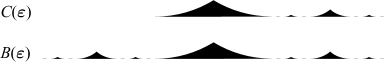
Figure 9: $\mu$ is the ratio $\operatorname{vol_{\text{$2$}}}(C(\varepsilon))/\operatorname{vol_{\text{$2$}}}(B(\varepsilon))$.

$$\mu:=\frac{A_{1}(\varepsilon_{k})+\tfrac{1}{2}\sum_{k=2}^{\infty}2^{k-1}A_{k}(\varepsilon_{k})}{\sum_{k=1}^{\infty}2^{k-1}A_{k}(\varepsilon_{k})}=\frac{A_{1}(\varepsilon_{k})+\sum_{k=2}^{\infty}2^{k-2}A_{k}(\varepsilon_{k})}{\sum_{k=1}^{\infty}2^{k-1}A_{k}(\varepsilon_{k})}\in(0,1).$$

Note that although this definition of $\mu$ initially appears to depend on $k$, the ratio in question is between two areas which have exactly the same proportion at each $\varepsilon_{k}$; this is a direct consequence of the self-similarity of the Koch curve. In other words, if $C(\varepsilon)$ is the area indicated in Fig. 9, then the relations

$$3C(\tfrac{\varepsilon}{3})=C(\varepsilon)\text{ and }3B(\tfrac{\varepsilon}{3})=B(\varepsilon)$$

show that $\mu$ is well-defined.

We now approximate $h(\varepsilon)$ by a function which shares its essential properties:

• $\displaystyle h(\varepsilon_{k})=\lim_{\vartheta\to 0^{-}}h(\varepsilon_{k}+\vartheta)=0$,

• $\displaystyle\lim_{\vartheta\to 0^{+}}h(\varepsilon_{k}+\vartheta)=\mu$,

where for $k=1,2,\dots$, $\varepsilon_{k}=\tfrac{3^{-k}}{\sqrt{3}}$ again. That is, $h(\varepsilon)$ goes from 0 to $\mu$ as $\varepsilon$ goes from $3^{-k}$ to $3^{-(k+1)}$. Using again the notation $x=-\log_{3}(\varepsilon\sqrt{3})$ and $\{x\}=x-[x]$, we see that the function

$$\tilde{h}(\varepsilon)=\mu\cdot\{-[x]-x\}$$ (6.3)

shares both of these properties but is much smoother. Indeed, $\tilde{h}(\varepsilon)$ only has points of nondifferentiability at each $\varepsilon_{k}$ and is otherwise a smooth logarithmic curve; see Fig. 10. The true $h(\varepsilon)$, by contrast, is a much more complex object that deserves further study in later work.

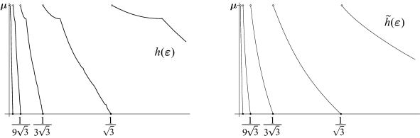
Figure 10: A comparison between the graph of the Cantor-like function $h$ and the graph of its approximation $\tilde{h}$.

Michel L. Lapidus,
Department of Mathematics, University of California, Riverside, CA 92521-0135

E-mail address: lapidus@math.ucr.edu

Erin P. J. Pearse,
Department of Mathematics, University of California, Riverside, CA 92521-0135

E-mail address: erin@math.ucr.edu

References

- [Fa] K. J. Falconer, Fractal Geometry — Mathematical Foundations and Applications, John Wiley, Chichester, 1990.
- [Gr] A. Gray, Tubes, second ed., Progress in Math., vol. 221, Birkhäuser, Boston, 2004.
- [HaLa] B. M. Hambly and M. L. Lapidus, Random fractal strings: Their zeta functions, complex dimensions and spectral asymptotics, Trans. Amer. Math. Soc. No. 1, 358 (2006), 285–314.
- [HeLa] C. Q. He and M. L. Lapidus, Generalized Minkowski content, spectrum of fractal drums, fractal strings and the Riemann zeta-function, Memoirs Amer. Math. Soc. No. 608, 127 (1997), 1–97.
- [Ki] J. Kigami, Analysis on Fractals, Cambridge Univ. Press, Cambridge, 2001.
- [L] S. P. Lalley, Packing and covering functions of some self-similar fractals, Indiana Univ. Math. J. 37 (1988), 699–709.
- [La1] M. L. Lapidus, Fractal drum, inverse spectral problems for elliptic operators and a partial resolution of the Weyl–Berry conjecture, Trans. Amer. Math. Soc. 325 (1991), 465–529.
- [La2] M. L. Lapidus, Spectral and fractal geometry: From the Weyl–Berry conjecture for the vibrations of fractal drums to the Riemann zeta-function, in: Differential Equations and Mathematical Physics (C. Bennewitz, ed.), Proc. Fourth UAB Internat. Conf. (Birmingham, March 1990), Academic Press, New York, 1992, pp. 151–182.
- [La3] M. L. Lapidus, Vibrations of fractal drums, the Riemann hypothesis, waves in fractal media, and the Weyl–Berry conjecture, in: Ordinary and Partial Differential Equations (B. D. Sleeman and R. J. Jarvis, eds.), vol. IV, Proc. Twelfth Internat. Conf. (Dundee, Scotland, UK, June 1992), Pitman Research Notes in Math. Series, vol. 289, Longman Scientific and Technical, London, 1993, pp. 126–209.
- [LaMa] M. L. Lapidus and H. Maier, The Riemann hypothesis and inverse spectral problems for fractal strings, J. London Math. Soc. (2) 52 (1995), 15–34.
- [LaPe1] M. L. Lapidus and E. P. J. Pearse, Curvature measures and tube formulas of compact sets, in preparation.
- [LaPe2] M. L. Lapidus and E. P. J. Pearse, Tube formulas and complex dimensions of self-similar tilings, in preparation.
- [LaPo1] M. L. Lapidus and C. Pomerance, The Riemann-zeta function and the one-dimensional Weyl–Berry conjecture for fractal drums, Proc. London Math. Soc. (3) 66 (1993), 41–69.
- [LaPo2] M. L. Lapidus and C. Pomerance, Counterexamples to the modifed Weyl–Berry conjecture on fractal drums, Math. Proc. Cambridge Philos. Soc. 119 (1996), 167–178.
-
[La-vF1]
M. L. Lapidus and M. van Frankenhuysen, Fractal Geometry and Number Theory: Complex dimensions of fractal strings and zeros of zeta functions, Birkhäuser, Boston, 2000.
(Second rev. and enl. ed. to appear in 2006.) - [La-vF2] M. L. Lapidus and M. van Frankenhuysen, Complex dimensions of self-similar fractal strings and Diophantine approximation, J. Experimental Math. No. 1, 12 (2003), 41–69.
- [La-vF3] M. L. Lapidus and M. van Frankenhuysen, Fractality, self-similarity and complex dimensions, in: Fractal Geometry and Applications: A Jubilee of Benoît Mandelbrot, Proc. Symp. Pure Math. 72, Part 1, Amer. Math. Soc., Providence, R.I., 2004, pp. 349–373.
- [Man] B. B. Mandelbrot, The Fractal Geometry of Nature, rev. and enl. ed., W.H. Freeman, New York, 1983.
- [Mat] P. Mattila, Geometry of Sets and Measures in Euclidean Spaces (Fractals and Rectifiability), Cambridge Univ. Press, Cambridge, 1995.
- [Pe] E. P. J. Pearse, Canonical self-similar tilings by IFS, preprint, Nov. 2005, 14 pages.
- [Sch] L. Schwartz, Théorie des Distributions, rev. and enl. ed., Hermann, Paris, 1966.
- [Tr] C. Tricot, Curves and Fractal Dimensions, Springer-Verlag, New York, 1995.
- [We] H. Weyl, On the volume of tubes, Amer. J. Math. 61 (1939), 461–472.
- [Zy] A. Zygmund, Trigonometric Series, Cambridge University Press, Cambridge, 1959.