Abstract

These lectures provide an informal introduction into the notions and tools used to analyze statistical properties of eigenvalues of large random Hermitian matrices. After developing the general machinery of orthogonal polynomial method, we study in most detail Gaussian Unitary Ensemble (GUE) as a paradigmatic example. In particular, we discuss Plancherel-Rotach asymptotics of Hermite polynomials in various regimes and employ it in spectral analysis of the GUE. In the last part of the course we discuss general relations between orthogonal polynomials and characteristic polynomials of random matrices which is an active area of current research.

1 Preface

Gaussian Ensembles of random Hermitian or real symmetric matrices always played a prominent role in the development and applications of Random Matrix Theory. Gaussian Ensembles are uniquely singled out by the fact that they belong both to the family of invariant ensembles, and to the family of ensembles with independent, identically distributed (i.i.d) entries. In general, mathematical methods used to treat those two families are very different.

In fact, all random matrix techniques and ideas can be most clearly and consistently introduced using Gaussian case as a paradigmatic example. In the present set of lectures we mainly concentrate on consequences of the invariance of the corresponding probability density function, leaving aside methods of exploiting statistical independence of matrix entries. Under these circumstances the method of orthogonal polynomials is the most adequate one, and for the Gaussian case the relevant polynomials are Hermite polynomials. Being mostly interested in the limit of large matrix sizes we will spend a considerable amount of time investigating various asymptotic regimes of Hermite polynomials, since the latter are main building blocks of various correlation functions of interest. In the last part of our lecture course we will discuss why statistics of characteristic polynomials of random Hermitian matrices turns out to be interesting and informative to investigate, and will make a contact with recent results in the domain.

The presentation is quite informal in the sense that I will not try to prove various statements in full rigor or generality. I rather attempt outlining the main concepts, ideas and techniques preferring a good illuminating example to a general proof. A much more rigorous and detailed exposition can be found in the cited literature. I will also frequently employ the symbol $\propto$. In the present set of lectures it always means that the expression following $\propto$ contains a multiplicative constant which is of secondary importance for our goals and can be restored when necessary.

2 Introduction

In these lectures we use the symbol ^T to denote matrix or vector transposition and the asterisk ^∗ to denote Hermitian conjugation. In the present section the bar $\overline{z}$ denotes complex conjugation.

Let us start with a square complex matrix $\hat{Z}$ of dimensions $N\times N$, with complex entries $z_{ij}=x_{ij}+iy_{ij},\,1\leq i,j\leq N$. Every such matrix can be conveniently looked at as a point in a $2N^{2}$-dimensional Euclidean space with real Cartesian coordinates $x_{ij},\,y_{ij}$, and the length element in this space is defined in a standard way as:

$$(ds)^{2}=\mbox{Tr}\left(d\hat{Z}d\hat{Z}^{*}\right)=\sum_{ij}dz_{ij}\overline{dz_{ij}}=\sum_{ij}\left[(dx)^{2}_{ij}+(dy)^{2}_{ij}\right].$$ (1)

As is well-known (see e.g.[1]) any surface embedded in an Euclidean space inherits a natural Riemannian metric from the underlying Euclidean structure. Namely, let the coordinates in a $n-$dimensional Euclidean space be $(x_{1},\ldots,x_{n})$, and let a $k-$dimensional surface embedded in this space be parameterized in terms of coordinates $(q_{1},\ldots,q_{k}),\,k\leq n$ as $x_{i}=x_{i}(q_{1},\ldots,q_{k}),\,i=1,\ldots n$. Then the Riemannian metric $g_{ml}=g_{lm}$ on the surface is defined from the Euclidean length element according to

$$(ds)^{2}=\sum_{i=1}^{n}(dx_{i})^{2}=\sum_{i=1}^{n}\left(\sum_{m=1}^{k}\frac{\partial x_{i}}{\partial q_{m}}dq_{m}\right)^{2}=\sum_{m,l=1}^{k}g_{mn}dq_{m}dq_{l}.$$ (2)

Moreover, such a Riemannian metric induces the corresponding integration measure on the surface, with the volume element given by

$$d\mu=\sqrt{|g|}dq_{1}\ldots dq_{k},\quad g=\det{\left(g_{ml}\right)_{l,m=1}^{k}}.$$ (3)

For $k=n$ these are just the familiar formulae for the lengths and volume associated with change of coordinates in an Euclidean space. For example, for $n=2$ we can pass from Cartesian coordinates $-\infty<x,\,y<\infty$ to polar coordinates $r>0$, $0\leq\theta<2\pi$ by $x=r\cos{\theta}$, $y=r\sin{\theta}$, so that $dx=dr\cos{\theta}-r\sin{\theta}d\theta$, $dy=dr\sin{\theta}+r\cos{\theta}d\theta$, and the Riemannian metric is defined by $(ds)^{2}=(dx)^{2}+(dy)^{2}=(dr)^{2}+r^{2}(d\theta)^{2}$. We find that $g_{11}=1,\,g_{12}=g_{21}=0,\,g_{22}=r^{2}$, and the volume element of the integration measure in the new coordinates is $d\mu=rdrd\theta$; as it should be. As the simplest example of a “surface” with $k<n=2$ embedded in such a two-dimensional space we consider a circle $r=R=const$. We immediately see that the length element $(ds)^{2}$ restricted to this “surface” is $(ds)^{2}=R^{2}(d\theta)^{2}$, so that $g_{11}=R^{2}$, and the integration measure induced on the surface is correspondingly $d\mu=Rd\theta$. The “surface” integration then gives the total “volume” of the embedded surface (i.e. circle length $2\pi R$).

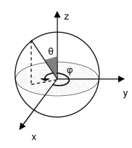
Figure 1: The spherical coordinates for a two dimensional sphere in the three-dimensional Euclidean space.

Similarly, we can consider a two-dimensional ($k=2$) sphere $R^{2}=x^{2}+y^{2}+z^{2}$ embedded in a three-dimensional Euclidean space $(n=3)$ with coordinates $x,y,z$ and length element $(ds)^{2}=(dx)^{2}+(dy)^{2}+(dz)^{2}$. A natural parameterization of the points on the sphere is possible in terms of the spherical coordinates $\phi,\theta$ (see Fig.  1)

$$x=R\sin{\theta}\cos{\phi},\,\,y=R\sin{\theta}\sin{\phi},\,\,z=R\cos{\theta};\quad 0\leq\theta\leq\pi,\,\,0\leq\phi<2\pi,$$

which results in $(ds)^{2}=R^{2}(d\theta)^{2}+R^{2}\sin^{2}{\theta}(d\phi)^{2}$. Hence the matrix elements of the metric are $g_{11}=R^{2},\,g_{12}=g_{21}=0,g_{22}=R^{2}\sin^{2}{\theta}$, and the corresponding “volume element” on the sphere is the familiar elementary area $d\mu=R^{2}\sin{\theta}d\theta d\phi$.

As a less trivial example to be used later on consider a $2-$dimensional manifold formed by $2\times 2$ unitary matrices $\hat{U}$ embedded in the $8$ dimensional Euclidean space of $Gl(2;C)$ matrices. Every such matrix can be represented as the product of a matrix $\hat{U}_{c}$ from the coset space $U(2)/U(1)\times U(1)$ parameterized by $k=2$ real coordinates $0\leq\phi<2\pi,\,0\leq\theta\leq\pi/2$, and a diagonal unitary matrix $U_{d}$, that is $\hat{U}=\hat{U}_{d}\hat{U}_{c}$, where

$$\hat{U_{c}}=\left(\begin{array}[]{cc}\cos{\theta}&-\sin{\theta}e^{-i\phi}\\ \sin{\theta}e^{i\phi}&\cos{\theta}\end{array}\right),\quad\hat{U_{d}}=\left(\begin{array}[]{cc}e^{-i\phi_{1}}&0\\ 0&e^{i\phi_{2}}\end{array}\right).$$ (4)

Then the differential $d\hat{U}$ of the matrix $\hat{U}=\hat{U}_{d}\hat{U}_{c}$ has the following form:

$$\hat{dU}=\left(\begin{array}[]{cc}-[d\theta\sin{\theta}+i\cos{\theta}d\phi_{1}]e^{-i\phi_{1}}&e^{-i(\phi_{1}+\phi)}[-d\theta\cos{\theta}+i(d\phi_{1}+d\phi)\sin{\theta}]\\ e^{i(\phi+\phi_{2})}[d\theta\cos{\theta}+i(d\phi+d\phi_{2})\sin{\theta}]&[-d\theta\sin{\theta}+id\phi_{2}\cos{\theta}]e^{i\phi_{2}}\end{array}\right),$$ (5)

which yields the length element and the induced Riemannian metric:

$$(ds)^{2}=\mbox{Tr}\left(d\hat{U}d\hat{U}^{*}\right)=2(d\theta)^{2}+(d\phi_{1})^{2}+(d\phi_{2})^{2}+2\sin^{2}{\theta}(d\phi)^{2}+2\sin^{2}{\theta}(d\phi\,d\phi_{1}+d\phi\,d\phi_{2}).$$ (6)

We see that the nonzero entries of the Riemannian metric tensor $g_{mn}$ in this case are $g_{11}=2,\,g_{22}=g_{33}=1,g_{44}=2\sin^{2}{\theta},\,g_{24}=g_{42}=g_{34}=g_{43}=\sin^{2}{\theta}$, so that the determinant $\det{[g_{mn}]}=4\sin^{2}{\theta}\cos^{2}{\theta}$. Finally, the induced integration measure on the group $U(2)$ is given by

$$d\mu(\hat{U})=2\sin{\theta}\cos{\theta}\,d\theta\,d\phi\,d\phi_{1}\,d\phi_{2}.$$ (7)

It is immediately clear that the above expression is invariant, by construction, with respect to multiplications $\hat{U}\to\hat{V}\hat{U}$, for any fixed unitary matrix $V$ from the same group. Therefore, Eq.(7) is just the Haar measure on the group.

We will make use of these ideas several times in our lectures. Let us now concentrate on the $N^{2}-$dimensional subspace of Hermitian matrices in the $2N^{2}-$ dimensional space of all complex matrices of a given size $N$. The Hermiticity condition $\hat{H}=\hat{H}^{*}\equiv\overline{\hat{H}^{T}}$ amounts to imposing the following restrictions on the coordinates: $x_{ij}=x_{ji},\,\,y_{ij}=-y_{ji}$. Such a restriction from the space of general complex matrices results in the length and volume element on the subspace of Hermitian matrices:

$$(ds)^{2}=\mbox{Tr}\left(d\hat{H}d\hat{H}^{*}\right)=\sum_{i}(dx_{ii})^{2}+2\sum_{i<j}\left[(dx_{ij})^{2}+(dy_{ij})^{2}\right]$$ (8)

$$d\mu(\hat{H})=2^{\frac{N(N-1)}{2}}\prod_{i}dx_{ii}\prod_{i<j}dx_{ij}dy_{ij}.$$ (9)

Obviously, the length element $(ds)^{2}=\mbox{Tr}d\hat{H}d\hat{H}^{*}$ is invariant with respect to an automorphism (a mapping of the space of Hermitian matrices to itself) by a similarity transformation $\hat{H}\to U^{-1}\hat{H}\hat{U}$, where $\hat{U}\in U(N)$ is any given unitary $N\times N$ matrix: $\hat{U}^{*}=\hat{U}^{-1}$. Therefore the corresponding integration measure $d\mu(\hat{H})$ is also invariant with respect to all such “rotations of the basis”.

The above-given measure $d\mu(\hat{H})$ written in the coordinates $x_{ii},\,x_{i<j},\,y_{i<j}$ is frequently referred to as the “flat measure”. Let us discuss now another, very important coordinate system in the space of Hermitian matrices which will be in the heart of all subsequent discussions. As is well-known, every Hermitian matrix $\hat{H}$ can be represented as

$$\hat{H}=\hat{U}\hat{\Lambda}\hat{U}^{-1},\quad\hat{\Lambda}=\mbox{diag}(\lambda_{1},\ldots,\lambda_{N}),\,\,\hat{U}^{*}\hat{U}=\hat{I},$$ (10)

where real $-\infty<\lambda_{k}<\infty,\,k=1,\ldots,N$ are eigenvalues of the Hermitian matrix, and rows of the unitary matrix $\hat{U}$ are corresponding eigenvectors. Generically, we can consider all eigenvalues to be simple (non-degenerate). More precisely, the set of matrices $\hat{H}$ with non-degenerate eigenvalues is dense and open in the $N^{2}$-dimensional space of all Hermitian matrices, and has full measure (see [3], p.94 for a formal proof). The correspondence $\hat{H}\to\left(\hat{U}\in U(N),\hat{\Lambda}\right)$ is, however, not one-to-one, namely $\hat{U}_{1}\hat{\Lambda}\hat{U}_{1}^{-1}=\hat{U}_{2}\hat{\Lambda}\hat{U}_{2}^{-1}$ if $\hat{U}^{-1}_{1}\hat{U}_{2}=\mbox{diag}\left(e^{i\phi_{1}},\ldots,e^{i\phi_{N}}\right)$ for any choice of the phases $\phi_{1},\ldots,\phi_{N}$. To make the correspondence one-to-one we therefore have to restrict the unitary matrices to the coset space $U(N)/U(1)\otimes\ldots\otimes U(1)$, and also to order the eigenvalues, e.g. requiring $\lambda_{1}<\lambda_{2}<\ldots<\lambda_{N}$. Our next task is to write the integration measure $d\mu(\hat{H})$ in terms of eigenvalues $\hat{\Lambda}$ and matrices $\hat{U}$. To this end, we differentiate the spectral decomposition $\hat{H}=\hat{U}\hat{\Lambda}\hat{U}^{*}$, and further exploit: $d\left(\hat{U}^{*}\hat{U}\right)=d\hat{U}^{*}\hat{U}+\hat{U}^{*}d\hat{U}=0$. This leads to

$$d\hat{H}=\hat{U}\left[d\hat{\Lambda}+\hat{U}^{*}d\hat{U}\hat{\Lambda}-\hat{\Lambda}\hat{U}^{*}d\hat{U}\right]\hat{U}^{*}.$$ (11)

Substituting this expression into the length element $(ds)^{2}$, see Eq.(8), and using the short-hand notation $\delta\hat{U}$ for the matrix $\hat{U}^{*}d\hat{U}$ satisfying anti-Hermiticity condition $\delta\hat{U}^{*}=-\delta\hat{U}$, we arrive at:

$$(ds)^{2}=\mbox{Tr}\left[\left(d\hat{\Lambda}\right)^{2}+2d\hat{\Lambda}\left(\delta\hat{U}\hat{\Lambda}-\hat{\Lambda}\delta\hat{U}\right)+\left(\delta\hat{U}\hat{\Lambda}\right)^{2}+\left(\hat{\Lambda}\delta\hat{U}\right)^{2}-2\delta\hat{U}\hat{\Lambda}^{2}\delta\hat{U}\right].$$ (12)

Taking into account that $\hat{\Lambda}$ is purely diagonal, and therefore the diagonal entries of the commutator $\left(\delta\hat{U}\hat{\Lambda}-\hat{\Lambda}\delta\hat{U}\right)$ are zero, we see that the second term in Eq.(12) vanishes. On the other hand, the third and subsequent terms when added up are equal to

$$2\mbox{Tr}\left[\delta\hat{U}\hat{\Lambda}\delta\hat{U}\hat{\Lambda}-\delta\hat{U}^{2}\hat{\Lambda}^{2}\right]=2\sum_{ij}\left[\delta U_{ij}\lambda_{j}\delta U_{ji}\lambda_{i}-\lambda_{i}^{2}\delta U_{ij}\delta U_{ji}\right]=-\sum_{ij}\left(\lambda_{i}-\lambda_{j}\right)^{2}\delta U_{ji}\delta U_{ij}\,,$$

which together with the first term yields the final expression for the length element in the “spectral” coordinates

$$(ds)^{2}=\sum_{i}\left(d\lambda_{i}\right)^{2}+\sum_{i<j}\left(\lambda_{i}-\lambda_{j}\right)^{2}\overline{\delta U_{ij}}\delta U_{ij}\,$$ (13)

where we exploited the anti-Hermiticity condition $-\delta U_{ji}=\overline{\delta U_{ij}}$. Introducing the real and imaginary parts $\delta U_{ij}=\delta p_{ij}+i\delta q_{ij}$ as independent coordinates we can calculate the corresponding integration measure $d\mu(\hat{H})$ according to the rule in Eq.(3), to see that it is given by

$$d\mu(\hat{H})=\prod_{i<j}\left(\lambda_{i}-\lambda_{j}\right)^{2}\prod_{i}d\lambda_{i}\times d{\cal M}(\hat{U})\,.$$ (14)

The last factor $d{\cal M}(U)$ stands for the part of the measure depending only on the $U-$variables. A more detailed consideration shows that, in fact, $d{\cal M}(\hat{U})\equiv d\mu(\hat{U})$, which means that it is given (up to a constant factor) by the invariant Haar measure on the unitary group $U(N)$. This fact is however of secondary importance for the goals of the present lecture.

Having an integration measure at our disposal, we can introduce a probability density function (p.d.f.) ${\cal P}(\hat{H})$ on the space of Hermitian matrices, so that ${\cal P}(\hat{H})d\mu(\hat{H})$ is the probability that a matrix $\hat{H}$ belongs to the volume element $d\mu(\hat{H})$. Then it seems natural to require for such a probability to be invariant with respect to all the above automorphisms, i.e. ${\cal P}(\hat{H})={\cal P}\left(\hat{U}^{*}\hat{H}\hat{U}\right)$. It is easy to understand that this “postulate of invariance” results in ${\cal P}$ being a function of $N$ first traces $\mbox{Tr}\hat{H}^{n},\,n=1,\ldots,N$ (the knowledge of first $N$ traces fixes the coefficients of the characteristic polynomial of $\hat{H}$ uniquely, and hence the eigenvalues. Therefore traces of higher order can always be expressed in terms of the lower ones). Of particular interest is the case

$${\cal P}(\hat{H})=C\exp{-Tr\,Q(\hat{H})},\quad Q(x)=a_{2j}x^{2j}+\ldots+a_{0},$$ (15)

where $2j\leq N$, the parameters $a_{2l}$ and $C$ are real constants, and $a_{2j}>0$. Observe that if we take

$$Q(x)=ax^{2}+bx+c,$$ (16)

then $e^{-Tr\,Q(\hat{H})}$ takes the form of the product

$$e^{-a\left[\sum_{i}x^{2}_{ii}+2\sum_{i<j}(x^{2}_{ij}+y^{2}_{ij})\right]}e^{-b\sum_{i}x_{ii}}e^{-cN}=e^{-cN}\prod_{i=1}^{N}\left(e^{-ax_{ii}^{2}-bx_{ii}}\right)\prod_{i<j}e^{-2ax_{ij}^{2}}\prod_{i<j}e^{-2ay_{ij}^{2}}.$$ (17)

We therefore see that the probability distribution of the matrix $\hat{H}$ can be represented as a product of factors, each factor being a suitable Gaussian distribution depending only on one variable in the set of all coordinates $x_{ii},\,x_{i<j},\,y_{i<j}$. Since the same factorization is valid also for the integration measure $d\mu(\hat{H})$, see Eq.(9), we conclude that all these $N^{2}$ variables are statistically independent and Gaussian-distributed.

A much less obvious statement is that if we impose simultaneously two requirements:

• The probability density function ${\cal P}(\hat{H})$ is invariant with respect to all conjugations $\hat{H}\to\hat{H}^{\prime}=U^{-1}\hat{H}\hat{U}$ by unitary matrices $\hat{U}$, that is ${\cal P}(\hat{H}^{\prime})={\cal P}(\hat{H})$; and

• the $N^{2}$ variables $x_{ii},\,x_{i<j},\,y_{i<j}$ are statistically independent, i.e.

  $${\cal P}(\hat{H})=\prod_{i=1}^{N}f_{i}(x_{ii})\prod_{i<j}^{N}f^{(1)}_{ij}(x_{ij})f^{(2)}_{ij}(y_{ij}),$$ (18)

then the function ${\cal P}(\hat{H})$ is necessarily of the form ${\cal P}(\hat{H})=Ce^{-\left(a\mbox{Tr}\hat{H}^{2}+b\mbox{Tr}\hat{H}+cN\right)}$, for some constants $a>0,\,b,\,c$. The proof for any $N$ can be found in [2], and here we just illustrate its main ideas for the simplest, yet nontrivial case $N=2$. We require invariance of the distribution with respect to the conjugation of $\hat{H}$ by $\hat{U}\in U(2)$, and first consider a particular choice of the unitary matrix $\hat{U}=\left(\begin{array}[]{cc}1&-\theta\\ \theta&1\end{array}\right)$ corresponding to $\phi=\phi_{1}=\phi_{2}=0$, and small values $\theta\ll 1$ in Eq.(4). In this approximation the condition $\hat{H}^{\prime}=U^{-1}\hat{H}\hat{U}$ amounts to

$$\left(\begin{array}[]{cc}x^{\prime}_{11}&x^{\prime}_{12}+iy^{\prime}_{12}\\ x^{\prime}_{12}-iy^{\prime}_{12}&x^{\prime}_{22}\end{array}\right)=\left(\begin{array}[]{cc}x_{11}+2\theta x_{12}&x_{12}+iy_{12}+\theta\left(x_{22}-x_{11}\right)\\ x_{12}-iy_{12}+\theta\left(x_{22}-x_{11}\right)&x_{22}-2\theta x_{12}\end{array}\right),$$ (19)

where we kept only terms linear in $\theta$. With the same precision we expand the factors in Eq.(18):

$$f_{1}(x^{\prime}_{1})=f_{1}(x_{1})\left[1+2\theta x_{12}\frac{1}{f_{1}}\frac{df_{1}}{dx_{11}}\right],\,\,\,f_{2}(x^{\prime}_{22})=f_{2}(x_{22})\left[1-2\theta x_{12}\frac{1}{f_{2}}\frac{df_{2}}{dx_{22}}\right]$$

$$f^{(1)}_{12}(x^{\prime}_{12})=f^{(1)}_{12}(x_{12})\left[1+\theta(x_{22}-x_{11})\frac{1}{f^{(1)}_{12}}\frac{df^{(1)}_{12}}{dx_{12}}\right],\,\,\,f^{(2)}_{12}(y^{\prime}_{21})=f^{(2)}_{12}(y_{12}).$$

The requirements of statistical independence and invariance amount to the product of the left-hand sides of the above expressions to be equal to the product of the right-hand sides, for any $\theta$. This is possible only if:

$$2x_{12}\left[\frac{d\ln{f_{1}}}{dx_{11}}-\frac{d\ln{f_{2}}}{dx_{22}}\right]+(x_{22}-x_{11})\frac{d\ln{f^{(1)}_{12}}}{dx_{12}}=0,$$ (20)

which can be further rewritten as

$$\frac{1}{(x_{22}-x_{11})}\left[\frac{d\ln{f_{1}}}{dx_{11}}-\frac{d\ln{f_{2}}}{dx_{22}}\right]=const=\frac{1}{2x_{12}}\frac{d\ln{f^{(1)}_{12}}}{dx_{12}},$$ (21)

where we used that the two sides in the equation above depend on essentially different sets of variables. Denoting $const_{1}=-2a$, we see immediately that

$$f^{(1)}_{12}(x_{12})\propto e^{-2ax^{2}_{12}},$$

and further notice that

$$\frac{d\ln{f_{1}}}{dx_{11}}+2ax_{11}=const_{2}=\frac{d\ln{f_{2}}}{dx_{22}}+2ax_{22}$$

by the same reasoning. Denoting $const_{2}=-b$, we find:

$$f_{1}(x_{11})\propto e^{-ax^{2}_{11}-bx_{11}},\quad f_{2}(x_{22})\propto e^{-ax^{2}_{22}-bx_{22}},$$ (22)

and thus we are able to reproduce the first two factors in Eq.(17). To reproduce the remaining factors we consider the conjugation by the unitary matrix $\hat{U_{d}}=\left(\begin{array}[]{cc}1-i\alpha&0\\ 0&1+i\alpha\end{array}\right)$, which corresponds to the choice $\theta=0,\,\phi_{1}=\phi_{2}=-\alpha=$ in Eq.(4), and again we keep only terms linear in the small parameter $\alpha\ll 1$. Within such a precision the transformation leaves the diagonal entries $x_{11},\,x_{22}$ unchanged, whereas the real and imaginary parts of the off-diagonal entries are transformed as

$$x^{\prime}_{12}=x_{12}-2\alpha y_{12},\quad y^{\prime}_{12}=y_{12}+2\alpha x_{12}.$$

In this case the invariance of the p.d.f. ${\cal P}(\hat{H})$ together with the statistical independence of the entries amount, after straightforward manipulations, to the condition

$$\frac{1}{x_{12}}\frac{d\ln{f^{(1)}_{12}}}{dx_{12}}=\frac{1}{y_{12}}\frac{d\ln{f^{(2)}_{12}}}{dy_{12}}$$

which together with the previously found $f^{(1)}_{12}(x_{12})$ yields

$$f^{(2)}_{12}(y_{12})\propto e^{-2ay^{2}_{12}},$$

completing the proof of Eq.(17).

The Gaussian form of the probability density function, Eq.(17), can also be found as a result of rather different lines of thought. For example, one may invoke an information theory approach a la Shanon-Khinchin and define the amount of information ${\cal I}[{\cal P}(\hat{H})]$ associated with any probability density function ${\cal P}(\hat{H})$ by

$${\cal I}[{\cal P}(\hat{H})]=-\int d\mu(\hat{H})\,{\cal P}(\hat{H})\ln{{\cal P}(\hat{H})}$$ (23)

This is a natural extension of the corresponding definition ${\cal I}[p_{1},\ldots,p_{m}]=-\sum_{l=1}^{m}p_{m}\ln{p_{m}}$ for discrete events $1,...,m$.

Now one can argue that in order to have matrices $\hat{H}$ as random as possible one has to find the p.d.f. minimizing the information associated with it for a certain class of ${\cal P}(H)$ satisfying some conditions. The conditions usually have a form of constraints ensuring that the probability density function has desirable properties. Let us, for example, impose the only requirement that the ensemble average for the two lowest traces $\mbox{Tr}\hat{H},\mbox{Tr}\hat{H}^{2}$ must be equal to certain prescribed values, say $E\left[\mbox{Tr}\hat{H}\right]=b$ and $E\left[\mbox{Tr}\hat{H}^{2}\right]=a>0$, where the $E\left[\ldots\right]$ stand for the expectation value with respect to the p.d.f. ${\cal P}(H)$. Incorporating these constraints into the minimization procedure in a form of Lagrange multipliers $\nu_{1},\nu_{2}$, we seek to minimize the functional

$${\cal I}[{\cal P}(\hat{H})]=-\int d\mu(\hat{H})\,{\cal P}(\hat{H})\left\{\ln{{\cal P}(\hat{H})}-\nu_{1}\mbox{Tr}\hat{H}-\nu_{2}\mbox{Tr}\hat{H}^{2}\right\}.$$ (24)

The variation of such a functional with respect to $\delta{\cal P}(\cal{H})$ results in

$$\delta{\cal I}[{\cal P}(\hat{H})]=-\int d\mu(\hat{H})\,\delta{\cal P}(\hat{H})\left\{1+\ln{{\cal P}(\hat{H})}-\nu_{1}\mbox{Tr}\hat{H}-\nu_{2}\mbox{Tr}\hat{H}^{2}\right\}=0$$ (25)

possible only if

$${\cal P}(\hat{H})\propto\exp\{\nu_{1}\mbox{Tr}\hat{H}+\nu_{2}\mbox{Tr}\hat{H}^{2}\}$$

again giving the Gaussian form of the p.d.f. The values of the Lagrange multipliers are then uniquely fixed by constants $a,b$, and the normalization condition on the probability density function. For more detailed discussion, and for further reference see [2], p.68.

Finally, let us discuss yet another construction allowing one to arrive at the Gaussian Ensembles exploiting the idea of Brownian motion. To start with, consider a system whose state at time $t$ is described by one real variable $x$, evolving in time according to the simplest linear differential equation $\frac{d}{dt}x=-x$ describing a simple exponential relaxation $x(t)=x_{0}e^{-t}$ towards the stable equilibrium $x=0$. Suppose now that the system is subject to a random additive Gaussian white noise $\xi(t)$ function of intensity $D$ , so that the corresponding equation acquires the form

$$\frac{d}{dt}x=-x+\xi(t),\quad E_{\xi}\left[\xi(t_{1})\xi(t_{1})\right]=D\delta(t_{1}-t_{2}),$$ (26)

where $E_{\xi}[\ldots]$ stands for the expectation value with respect to the random noise. The main characteristic property of a Gaussian white noise process is the following identity:

$$E_{\xi}\left[\exp\left\{\int_{a}^{b}\xi(t)v(t)dt\right\}\right]=\exp\left\{\frac{D}{2}\int_{a}^{b}v^{2}(t)dt\right\}$$ (27)

valid for any (smooth enough) test function $v(t)$. This is just a direct generalization of the standard Gaussian integral identity:

$$\int_{-\infty}^{\infty}\,\frac{dq}{\sqrt{2\pi a}}\,e^{-\frac{1}{2a}q^{2}+qb}=e^{\frac{ab^{2}}{2}}.$$ (28)

valid for $\mbox{Re}\,a>0$, and any (also complex) parameter $b$.

For any given realization of the Gaussian random process $\xi(t)$ the solution of the stochastic differential equation Eq.(26) is obviously given by

$$x(t)=e^{-t}\left[x_{0}+\int_{0}^{t}e^{\tau}\xi(\tau)d\tau\right].$$ (29)

This is a random function, and our main goal is to find the probability density function ${\cal P}(t,x)$ for the variable $x(t)$ to take value $x$ at any given moment in time $t$, if we know surely that $x(0)=x_{0}$. This p.d.f. can be easily found from the characteristic function

$${\cal F}(t,q)=E_{\xi}\left[e^{-iqx(t)}\right]=\exp\left\{-iqx_{0}e^{-t}-\frac{Dq^{2}}{4}(1-e^{-2t})\right\}$$ (30)

obtained by using Eqs. (27) and (29). The p.d.f. is immediately recovered by employing the inverse Fourier transform:

$${\cal P}(t,x)=\int_{-\infty}^{\infty}\frac{dq}{2\pi}e^{iqx}E_{\xi}\left[e^{-iqx(t)}\right]=\frac{1}{\sqrt{\pi D(1-e^{-2t})}}\exp\left\{-\frac{\left(x-x_{0}e^{-t}\right)^{2}}{D(1-e^{-2t})}\right\}.$$ (31)

The formula Eq.(31) is called the Ornstein-Uhlenbeck (OU) probability density function, and the function $x(t)$ satisfying the equation Eq.(26) is known as the O-U process. In fact, such a process describes an interplay between the random “kicks” forcing the system to perform a kind of Brownian motion and the relaxation towards $x=0$. It is easy to see that when time grows the OU p.d.f. “forgets” about the initial state and tends to a stationary (i.e. time-independent) universal Gaussian distribution:

$${\cal P}(t\to\infty,x)=\frac{1}{\sqrt{\pi D}}\exp\left\{-\frac{x^{2}}{D}\right\}.$$ (32)

Coming back to our main topic, let us consider $N^{2}$ independent OU processes: $N$ of them denoted as

$$\frac{d}{dt}x_{i}=-x_{i}+\xi_{i}(t),\quad 1\leq i\leq N$$ (33)

and the rest $N(N-1)$ given by

$$\frac{d}{dt}x_{ij}=-x_{ij}+\xi^{(1)}_{ij}(t),\quad\frac{d}{dt}y_{ij}=-y_{ij}+\xi^{(2)}_{ij}(t),$$ (34)

where the indices satisfy $\quad 1\leq i<j\leq N$. Stochastic processes $\xi(t)$ in the above equations are taken to be all mutually independent Gaussian white noises characterized by the correlation functions:

$$E_{\xi}\left[\xi_{i_{1}}(t_{1})\xi_{i_{2}}(t_{2})\right]=2D\delta_{i_{1},i_{2}}\delta(t_{1}-t_{2}),\,\,E_{\xi}\left[\xi^{\sigma_{1}}_{ij}(t_{1})\xi^{\sigma_{2}}_{kl}(t_{2})\right]=D\delta_{\sigma_{1},\sigma_{2}}\delta_{i,k}\delta_{j,l}\delta(t_{1}-t_{2}).$$ (35)

As initial values $x_{i}(0),x_{ij}(0),y_{ij}(0)$ for each OU process we choose diagonal and off-diagonal entries $H_{ii}^{(0)},\,\,i=1,\ldots,N$ and $\mbox{Re}H_{i<j}^{(0)},\,\mbox{Im}H_{i<j}^{(0)}$ of a fixed $N\times N$ Hermitian matrix $\hat{H}^{(0)}$. Let us now consider the Hermitian matrix $\hat{H}(t)$ whose entries are $H_{ii}(t)=x_{i}(t),\,H_{i<j}(t)=x_{i<j}(t)+iy_{i<j}(t)$ for any $t\geq 0$. It is immediately clear that the joint p.d.f. ${\cal P}\left(t,\hat{H}\right)$ of the entries of such a matrix $\hat{H}(t)$ will be given for any $t\geq 0$ by the OU-type formula:

$${\cal P}(t,\hat{H})\propto Const\times\frac{1}{\sqrt{(1-e^{-2t})^{N^{2}}}}\exp\left\{-\frac{1}{D(1-e^{-2t})}\mbox{Tr}\left(\hat{H}-\hat{H}_{0}e^{-t}\right)^{2}\right\}.$$ (36)

In the limit $t\to\infty$ this p.d.f. converges to a stationary, $t-$independent expression

$${\cal P}(t,\hat{H})\propto C\,e^{-\frac{1}{D}\mbox{Tr}\hat{H}^{2}}$$ (37)

independent of the initial matrix $\hat{H}_{0}$. We see therefore that the familiar Gaussian ensemble in the space of Hermitian matrices arises as the result of the stochastic relaxation from any initial condition, in particular, from any diagonal matrix with uncorrelated entries. In the next step one may try to deduce the stochastic dynamics of the eigenvalues of the corresponding matrices. Those eigenvalues obviously evolve from completely uncorrelated to highly correlated patterns. This very interesting set of question goes beyond our present goals and we refer to [2] for an introduction into the problem.

After specifying the probability density function ${\cal P}(H)$ the main question of interest is to characterize the statistical properties of the sequence of eigenvalues $\lambda_{1},\ldots,\lambda_{N}$ of $\hat{H}$. A convenient way of doing this is to start with the joint p.d.f. of all these eigenvalues. Because of the “rotational invariance” assumption the function ${\cal P}(\hat{H})$ depends in fact only on the eigenvalues, for example for the “symmetric” Gaussian case $b=0$ we have ${\cal P}(\hat{H})\propto e^{-a\sum_{i=1}^{N}\lambda_{i}^{2}}$. Moreover, we have seen that the integration measure $d\mu(\hat{H})$ when expressed in terms of eigenvalues and eigenvectors effectively factorizes, see Eq.(14). Collecting all these facts we arrive at the conclusion, that the relevant joint p.d.f of all eigenvalues can be always written, up to a normalization constant, as

$${\cal P}(\lambda_{1},\ldots,\lambda_{N})\,d\lambda_{1}\ldots d\lambda_{N}\propto e^{-\sum_{i=1}^{N}Q(\lambda_{i})}\prod_{i<j}\left(\lambda_{i}-\lambda_{j}\right)^{2}\,\,d\lambda_{1}\ldots d\lambda_{N}$$ (38)

for a general, non-gaussian weight $e^{-\mbox{Tr}Q(\hat{H})}$. We immediately see that the presence of the “Jacobian factor” $\prod_{i<j}\left(\lambda_{i}-\lambda_{j}\right)^{2}$ is responsible of the fact that the eigenvalues are correlated in a non-trivial way. In what follows we are going to disregard the fact that eigenvalues $\lambda_{i}$ were initially put in increasing order. More precisely, for any symmetric function $f$ of $N$ real variables $\lambda_{1},\ldots,\lambda_{N}$ the expected value will be calculated as

$$\int_{{\bf R}^{N}}f(\lambda_{1},\ldots,\lambda_{N}){\cal P}(\lambda_{1},\ldots,\lambda_{N})d\lambda_{1}\,\ldots\,d\lambda_{N}.$$

Indeed, with p.d.f. being symmetric with respect to permutations of the eigenvalue set, disregarding the ordering amounts to a simple multiplicative combinatorial factor $n!$ in the normalization constant.

Our main goal is to extract the information about these eigenvalue correlations in the limit of large size $N$. From this point of view it is pertinent to discuss a few quantitative measures frequently used to characterize correlations in sequences of real numbers.

3 Characterization of Spectral Sequences

Let $-\infty<\lambda_{1},\lambda_{2},\ldots,\lambda_{N}<\infty$ be the positions of $N$ points on the real axis, characterized by the joint probability density function (JPDF)

$${\cal P}(\lambda_{1},\lambda_{2},\ldots,\lambda_{N})\,\,d\lambda_{1}\,\ldots\,d\lambda_{N}$$

of having, regardless of labelling, one point in the interval $[\lambda_{1},\lambda_{1}+d\lambda_{1}]$, another in the interval $[\lambda_{2},\lambda_{2}+d\lambda_{2}]$,…, another in $[\lambda_{N},\lambda_{N}+d\lambda_{N}]$. Since in this section we deal exclusively with real variables, the bar will stand for the expectation value with respect to such a JPDF.

The statistical properties of the sequence $\{\lambda_{i}\}$ are conveniently characterized by the set of $n-$point correlation functions, defined as

$${\cal R}_{n}(\lambda_{1},\lambda_{2},\ldots,\lambda_{n})=\frac{N!}{(N-n)!}\int{\cal P}(\lambda_{1},\lambda_{2},\ldots,\lambda_{N})\,\,d\lambda_{n+1}\,\ldots\,d\lambda_{N}.$$ (39)

It is obvious from this definition that the lower correlation functions can be obtained from the higher-order ones:

$${\cal R}_{n}(\lambda_{1},\lambda_{2},\ldots,\lambda_{n})=\frac{1}{(N-n)}\int{\cal R}_{n+1}(\lambda_{1},\lambda_{2},\ldots,\lambda_{n+1})\,\,d\lambda_{n+1}.$$ (40)

To provide a more clear interpretation of these correlation functions we relate them to the statistics of the number $N_{B}$ of points of the sequence $\{\lambda_{i}\}$ within any set $B$ of the real axis (e.g an interval $[a,b]$). Let $\chi_{B}(x)$ be the characteristic function of the set $B$, equal to unity if $x\in B$ and zero otherwise. Introduce the exact density function $\rho_{N}(\lambda)$ of the points $\{\lambda_{i}\}$ around the point $\lambda$ on the real axis. It can be conveniently written using the Dirac’s $\delta-$function as $\rho_{N}(\lambda)=\sum_{i=1}^{N}\delta(\lambda-\lambda_{i})$. Then $N_{B}=\int\chi_{B}(\lambda)\rho_{N}(\lambda)d\lambda$.

On the other hand, consider

$$\int_{B}{\cal R}_{1}(\lambda_{1})d\lambda_{1}=\int\chi_{B}(\lambda_{1}){\cal R}_{1}(\lambda_{1})d\lambda_{1}=N\int\chi_{B}(\lambda_{1}){\cal P}(\lambda_{1},\lambda_{2},\ldots,\lambda_{N})\,\,d\lambda_{1}\,\ldots\,d\lambda_{N}$$

$$=\int\,\sum_{i=1}^{N}\chi_{B}(\lambda_{i}){\cal P}(\lambda_{1},\lambda_{2},\ldots,\lambda_{N})\,\,d\lambda_{1}\,\ldots\,d\lambda_{N}$$ (41)

and therefore

$$\int_{B}{\cal R}_{1}(\lambda_{1})d\lambda_{1}=\overline{N_{B}}=\mbox{expectation of the number of points in B}.$$ (42)

Similarly, consider

$$\int\chi_{B}(\lambda_{1})\chi_{B}(\lambda_{2}){\cal R}_{2}(\lambda_{1},\lambda_{2})d\lambda_{1}d\lambda_{2}=N(N-1)\int\chi_{B}(\lambda_{1})\chi_{B}(\lambda_{2}){\cal P}(\lambda_{1},\lambda_{2},\ldots,\lambda_{N})\,\,d\lambda_{1}\,\ldots\,d\lambda_{N}$$

$$=\int\,\sum_{i\neq j}^{N}\chi_{B}(\lambda_{i})\chi_{B}(\lambda_{j}){\cal P}(\lambda_{1},\lambda_{2},\ldots,\lambda_{N})\,\,d\lambda_{1}\,\ldots\,d\lambda_{N},$$ (43)

which can be interpreted as

$$\int_{B\times B}{\cal R}_{2}(\lambda_{1},\lambda_{2})d\lambda_{1}d\lambda_{2}=\mbox{expectation of the number of pairs of points in B}$$ (44)

where if, say, $\lambda_{1}$ and $\lambda_{2}$ are in $B$, then the pair $\{1,2\}$ and $\{2,1\}$ are both counted.

To relate the two-point correlation function to the variance of $N_{B}$ we notice that in view of Eq.(42) the one-point correlation function ${\cal R}_{1}(\lambda)$ coincides with the mean density $\overline{\rho}_{N}(\lambda)$ of the points $\{\lambda_{i}\}$ around the point $\lambda$ on the real axis. Similarly, write the mean square $\overline{N^{2}_{B}}$

$$\overline{N^{2}_{B}}=\int\chi_{B}(\lambda)\chi_{B}(\lambda^{\prime})\overline{\rho_{N}(\lambda)\rho_{N}(\lambda^{\prime})}\,\,d\lambda d\lambda^{\prime}$$ (45)

and notice that

$$\overline{\rho_{N}(\lambda)\rho_{N}(\lambda^{\prime})}=\overline{\sum_{ij}\delta(\lambda-\lambda_{i})\delta(\lambda^{\prime}-\lambda_{j})}=\delta(\lambda-\lambda^{\prime})\overline{\sum_{i}\delta(\lambda-\lambda_{i})}+\overline{\sum_{i\neq j}\delta(\lambda-\lambda_{i})\delta(\lambda^{\prime}-\lambda_{j})}$$

$$=\delta(\lambda-\lambda^{\prime}){\cal R}_{1}(\lambda)+{\cal R}_{2}(\lambda,\lambda^{\prime}).$$ (46)

In this way we arrive at the relation:

$$\overline{N^{2}_{B}}=\overline{N_{B}}+\int_{B\times B}{\cal R}_{2}(\lambda,\lambda^{\prime})\,\,d\lambda d\lambda^{\prime}.$$ (47)

In fact, it is natural to introduce the so-called “number variance” statistics $\Sigma_{2}(B)=\overline{N^{2}_{B}}-\left[\overline{N_{B}}\right]^{2}$ describing the variance of the number of points of the sequence inside the set $B$. Obviously,

$$\Sigma_{2}(B)=\overline{N_{B}}+\int_{B\times B}\left[{\cal R}_{2}(\lambda,\lambda^{\prime})-{\cal R}_{1}(\lambda){\cal R}_{1}(\lambda^{\prime})\right]\,\,d\lambda d\lambda^{\prime}\equiv\overline{N_{B}}-\int_{B\times B}Y_{2}(\lambda,\lambda^{\prime})\,\,d\lambda d\lambda^{\prime}$$ (48)

where we introduced the so-called cluster function $Y_{2}(\lambda,\lambda^{\prime})={\cal R}_{1}(\lambda){\cal R}_{1}(\lambda^{\prime})-{\cal R}_{2}(\lambda,\lambda^{\prime})$ frequently used in applications.

Finally, in principle the knowledge of all $n-$point correlation functions provides one with the possibility of calculating an important characteristic of the spectrum known as the “hole probability” $A(L)$. This quantity is defined as the probability for a random matrix to have no eigenvalues in the interval $(-L/2,L/2)$ . Define $\chi_{L}(\lambda)$ to be the characteristic function of this interval. Obviously,

$$A(L)=\int\ldots\int\,{\cal P}(\lambda_{1},\ldots,\lambda_{N})\prod_{k=1}^{N}\left(1-\chi_{L}(\lambda_{k})\right)\,\,d\lambda_{1}\ldots d\lambda_{N}$$ (49)

$$=\sum_{j=0}^{N}(-1)^{j}\,\int\ldots\int\,{\cal P}(\lambda_{1},\ldots,\lambda_{N})h_{j}\left\{\chi_{L}(\lambda_{1}),\ldots,\chi_{L}(\lambda_{N})\right\}\,\,d\lambda_{1}\ldots d\lambda_{N},$$ (50)

where $h_{j}\{x_{1},\ldots,x_{N}\}$ is the $j-th$ symmetric function:

$$h_{0}\{x_{1},\ldots,x_{N}\}=1,\,\,h_{1}\{x_{1},\ldots,x_{N}\}=\sum_{i=1}^{N}x_{i}\,,$$

$$h_{2}\{x_{1},\ldots,x_{N}\}=\sum_{i<j}^{N}x_{i}x_{j},\quad\ldots,\quad h_{N}\{x_{1},\ldots,x_{N}\}=x_{1}x_{2}\ldots x_{N}.$$

Now, for $1\leq j\leq N$

$$\int\ldots\int\,\prod_{k=1}^{j}\chi_{L}(\lambda_{k})\,\,{\cal P}(\lambda_{1},\ldots,\lambda_{N})d\lambda_{1}\ldots d\lambda_{N}$$

$$=\frac{(N-j)!}{N!}\int\ldots\int\prod_{k=1}^{j}\chi_{L}(\lambda_{k}){\cal R}_{j}(\lambda_{1},\ldots,\lambda_{j})\,\,d\lambda_{1}\ldots d\lambda_{j}$$ (51)

$$=\frac{(N-j)!}{N!}\int_{|x_{1}|<L/2}\ldots\int_{|x_{j}|<L/2}\,{\cal R}_{j}(\lambda_{1},\ldots,\lambda_{j})\,\,d\lambda_{1}\ldots d\lambda_{j}.$$ (52)

As $h_{j}$ contains $\left(\begin{array}[]{c}N\\ j\end{array}\right)$ terms and as ${\cal R}_{j}(\lambda_{1},\ldots,\lambda_{j})$ is invariant under permutations of the arguments, it follows that

$$\int\ldots\int{\cal P}(\lambda_{1},\ldots,\lambda_{N})h_{j}\left\{\chi_{L}(\lambda_{1})\ldots\chi_{L}(\lambda_{N})\right\}\,\,d\lambda_{1}\ldots d\lambda_{j}$$

$$=\frac{(N-j)!}{N!}\left(\begin{array}[]{c}N\\ j\end{array}\right)\int_{|x_{1}|<L/2}\ldots\int_{|x_{j}|<L/2}\,{\cal R}_{j}(\lambda_{1},\ldots,\lambda_{j})\,\,d\lambda_{1}\ldots d\lambda_{j}=$$ (55)

$$\frac{1}{j!}\int_{|x_{1}|<L/2}\ldots\int_{|x_{j}|<L/2}\,{\cal R}_{j}(\lambda_{1},\ldots,\lambda_{j})\,\,d\lambda_{1}\ldots d\lambda_{j}.$$ (56)

Thus, we arrive at the following relation between the hole probability and the $n-$point correlation functions:

$$A(L)=\sum_{j=0}^{N}\frac{(-1)^{j}}{j!}\int_{-L/2}^{L/2}\ldots\int_{-L/2}^{L/2}\,{\cal R}_{j}(\lambda_{1},\ldots,\lambda_{j})\,\,d\lambda_{1}\ldots d\lambda_{j}.$$ (57)

One of the main goals of this set of lectures is to develop a method allowing to evaluate all the $n-$point correlation functions of the eigenvalues for any JPDF corresponding to unitary invariant ensembles of the form Eq.(15). After that we will concentrate on a particular case of Gaussian weight and will investigate the limiting behaviour of the kernel function $K_{n}(\lambda,\lambda^{\prime})$ as $N\to\infty$. But even before doing this it is useful to keep in mind for reference purposes the results corresponding to completely uncorrelated (a.k.a. Poissonian) spectra. Those are described by a sequence of real points $\lambda_{1},\ldots,\lambda_{N}$, characterized by the fully factorized JPDF:

$${\cal P}(\lambda_{1},\lambda_{2},\ldots,\lambda_{N})\,\,=p(\lambda_{1})\,\ldots\,p(\lambda_{N}).$$ (58)

The normalization condition requires $\int_{-\infty}^{\infty}p(\lambda)\,d\lambda=1$, and we further assume $p(\lambda)$ to be a smooth enough integrable function. Obviously, for this case

$${\cal R}_{n}(\lambda_{1},\lambda_{2},\ldots,\lambda_{n})=\frac{N!}{(N-n)!}p(\lambda_{1})\,\ldots\,p(\lambda_{n}).$$ (59)

In particular, ${\cal R}_{n}(\lambda)=Np(\lambda)$ which is just the mean density $\overline{\rho(\lambda)}$ of points $\{\lambda_{i}\}$ around the point $\lambda$ on the real axis, and ${\cal R}_{n}(\lambda_{1},\lambda_{2})=N(N-1)p(\lambda_{1})p(\lambda_{2})$, etc.. From this we easily find for the number of levels in the domain $B$ and for its mean square:

$$\overline{N_{B}}=N\int_{B}p(\lambda)\,d\lambda,\quad\overline{N^{2}_{B}}=\overline{N_{B}}(N-1)/N+\left[\overline{N_{B}}\right]^{2}$$ (60)

and for the hole probability

$$A(L)=\sum_{j=0}^{N}\frac{(-1)^{j}}{j!}\frac{N!}{(N-j)!}\left[\int_{-L/2}^{L/2}p(\lambda)\,d\lambda\right]^{j}=\left[1-\int_{-L/2}^{L/2}p(\lambda)\,d\lambda\right]^{N}.$$ (61)

Finally, let us specify $B$ to be the interval $[-L/2,L/2]$ around the origin, and being interested mainly in large $N\gg 1$ consider the length $L$ comparable with the mean spacing between neighbouring points in the sequence $\{\lambda_{i}\}$ close to the origin, given by $\Delta\equiv\left[\overline{\rho(0)}\right]^{-1}=1/[Np(0)]$. In other words $s=L/\Delta=LNp(0)$ stays finite when $N\to\infty$. On the other hand, for large enough $N$ the function $p(\lambda)$ can be considered practically constant through the interval of the length $L=O(1/N)$, and therefore the mean number of points of the sequence $\{\lambda_{i}\}$ inside the interval $[-L/2,L/2]$ will be asymptotically given by $\overline{N(s)}\approx N\,L\,p(0)=s$. Similarly, using Eq.(60) one can easily calculate the “number variance” $\Sigma_{2}(s)=\overline{N^{2}_{[-\frac{L}{2},\frac{L}{2}]}}-\left[\overline{N_{[-\frac{L}{2},\frac{L}{2}]}}\right]^{2}=(N-1)\int_{-L/2}^{L/2}p(\lambda)\,d\lambda\approx s$. In the same approximation the hole probability, Eq.(61), tends asymptotically to $A(s)\approx e^{-s}$. Later on we shall compare these results with the corresponding behaviour emerging from the random matrix calculations.

4 The method of orthogonal polynomials

In the heart of the method developed mainly by Dyson, Mehta and Gaudin lies an “integrating-out” Lemma [2]. In presenting this material I follow very closely [3], pp.103-105.

• Let $J_{n}=J_{n}({\bf x})=(J_{ij})_{1\leq i,j\leq n}$ be an $n\times n$ matrix whose entries depend on a real vector ${\bf x}=(x_{1},x_{2},\ldots,x_{n})$ and have the form $J_{ij}=f(x_{i},x_{j})$, where $f$ is some (in general, complex-valued) function satisfying for some measure $d\mu(x)$ the “reproducing kernel” property:

  $$\int f(x,y)f(y,z)\,d\mu(y)=f(x,z).$$ (62)

  Then

  $$\int\mbox{det}\,J_{n}({\bf x})\,d\mu(x_{n})=[q-(n-1)]\mbox{det}\,J_{n-1}$$ (63)

  where $q=\int f(x,x)\,d\mu(x)$, and the matrix $J_{n-1}=(J_{ij})_{1\leq i,j\leq n-1}$ have the same functional form as $J_{n}$ with ${\bf x}$ replaced by $(x_{1},x_{2},\ldots,x_{n-1}).$

Before giving the idea of the proof for an arbitrary $n$ it is instructive to have a look on the simplest case $n=2$, when

$$J_{2}=\left(\begin{array}[]{cc}f(x_{1},x_{1})&f(x_{1},x_{2})\\ f(x_{2},x_{1})&f(x_{2},x_{2})\end{array}\right),\quad\mbox{hence}\quad\det{J_{n}}=f(x_{1},x_{1})f(x_{2},x_{2})-f(x_{1},x_{2})f(x_{2},x_{1}).$$

Integrating the latter expression over $x_{2}$, and using the “reproducing kernel” property, we immediately see that the result is indeed just $(q-1)f(x,x)=(q-1)\det{J_{1}}$ in full agreement with the statement of the Lemma.

For general $n$ one should follow essentially the same strategy and expand the determinant as a sum over $n!$ permutations $P_{n}(\sigma)=(\sigma_{1},\ldots\sigma_{n})$ of the index set $1,\ldots,n$ as

$$\int\mbox{det}\,J_{n}({\bf x})\,d\mu(x_{n})=\sum_{P_{n}}(-1)^{P_{n}}\int f(x_{1},x_{\sigma_{1}})\ldots f(x_{n},x_{\sigma_{n}})\,d\mu(x_{n}),$$ (64)

where $(-1)^{P_{n}}$ stands for the sign of permutations. Now, we classify the terms in the sum according to the actual value of the index $\sigma_{n}=k,\,k=1,2,\ldots,n$. Consider first the case $\sigma_{n}=n$, when effectively only the last factor $f(x_{n},x_{n})$ in the product is integrated yielding $d$ upon the integration. Summing up over the remaining $(n-1)!$ permutations $P_{n-1}(\sigma)$ of the index set $(1,2,...,n-1)$ we see that:

$$\sum_{P_{n-1}}(-1)^{P_{n}}\int\,f(x_{1},x_{\sigma_{1}})\ldots f(x_{n},x_{n})\,d\mu(x_{n})=q\sum_{P_{n-1}}(-1)^{P_{n-1}}\,f(x_{1},x_{\sigma_{1}})\ldots f(x_{n-1},x_{\sigma_{n-1}}),$$

which is evidently equal to $q\det{J_{n-1}}$. Now consider $(n-1)!$ terms with $\sigma_{n}=k<n$, when we have $\sigma_{j}=n$ for some $j<n$. For every such term we have by the “reproducing property”

$$\int\,f(x_{1},x_{\sigma_{1}})\ldots f(x_{j},x_{n})\ldots f(x_{n},x_{k})\,d\mu(x_{n})=f(x_{1},x_{\sigma_{1}})\ldots f(x_{j},x_{k})\ldots f(x_{n-1},x_{\sigma_{n-1}}).$$

Therefore

$$\int\mbox{det}\,J_{n}({\bf x})\,d\mu(x_{n})=q\det{J_{n-1}}+\sum_{k=1}^{n-1}\sum_{P_{n}:\sigma_{n}=k)}(-1)^{P_{n}}f(x_{1},x_{\sigma_{1}})\ldots f(x_{j},x_{k})\ldots f(x_{n-1},x_{\sigma_{n-1}}).$$ (65)

It is evident that the structure and the number of terms is as required, and the remaining task is to show that the summation over all possible $(n-1)!$ permutation of the index set for fixed $k$ yields always $-\det{J_{n-1}}$, see [3]. Then the whole expression is indeed equal to $[q-(n-1)]\det{J_{n-1}}$ as required.

Our next step is to apply this Lemma to calculating the $n-$point correlation functions of the eigenvalues $\lambda_{1},\ldots,\lambda_{n}$ starting from the JPDF, Eq.(38).

For this we notice that

$$\prod_{i<j}^{N}(\lambda_{i}-\lambda_{j})=(-1)^{\frac{N(N-1)}{2}}\det{\left(\begin{array}[]{ccc}1&\ldots&1\\ \lambda_{1}&\ldots&\lambda_{N}\\ .&.&.\\ .&.&.\\ .&.&.\\ \lambda^{N-1}_{1}&\ldots&\lambda^{N-1}_{N}\end{array}\right)}\equiv\Delta_{N}(\lambda_{1},\ldots,\lambda_{N}),$$ (66)

where the determinant in the right-hand side is the famous van der Monde determinant. Since the determinant cannot change upon linearly combining its rows, the entries $\lambda_{i}^{k}$ in $(k+1)-th$ row of the van der Monde determinant can be replaced, up to a constant factor $a_{0}a_{1}...a_{N-1}$, by a polynomial of degree $k$ of the form: $\pi_{k}(\lambda_{i})=a_{k}\lambda_{i}^{k}+\mbox{any polynomial in }\,\lambda_{i}\,\mbox{of degree less than k}$, with any choice of the coefficients $a_{l},\,l=0,\ldots,k$. Therefore:

$$\prod_{i<j}^{N}(\lambda_{i}-\lambda_{j})=\frac{(-1)^{\frac{N(N-1)}{2}}}{a_{0}a_{1}...a_{N-1}}\det{\left(\begin{array}[]{ccc}\pi_{0}(\lambda_{1})&\ldots&\pi_{0}(\lambda_{N})\\ \pi_{1}(\lambda_{1})&\ldots&\pi_{1}(\lambda_{N})\\ .&.&.\\ .&.&.\\ .&.&.\\ \pi_{N-1}(\lambda_{1})&\ldots&\pi_{N-1}(\lambda_{1})\end{array}\right)}\equiv\frac{(-1)^{\frac{N(N-1)}{2}}}{a_{0}a_{1}...a_{N-1}}\det{\left(\pi_{i-1}(\lambda_{j})\right)_{1\leq i,j\leq N}}.$$ (67)

Multiplying every entry in $j_{th}$ column in the above determinant with the factor $e^{-\frac{1}{2}Q(\lambda_{j})}$ we see that the JPDF can be conveniently written, up to a multiplicative constant, as

$${\cal P}(\lambda_{1},\ldots,\lambda_{N})\propto\left[\det{\left(e^{-\frac{1}{2}Q(\lambda_{j})}\pi_{i-1}(\lambda_{j})\right)_{1\leq i,j\leq N}}\right]^{2}.$$ (68)

If we let $\hat{A}$ be the matrix with the entries $A_{ij}=\left(\phi_{i-1}(x_{j})\right)_{1\leq i,j\leq N}$, then

$$[\det{A}]^{2}=\det{\hat{A}^{T}\hat{A}}=\det{\left(\sum_{j=1}^{n}A_{ji}A_{jk}\right)}.$$ (69)

This implies the following form of the JPDF:

$${\cal P}(\lambda_{1},\ldots,\lambda_{N})\propto\det{\left(\sum_{j=1}^{N}\phi_{j-1}(\lambda_{i})\phi_{j-1}(\lambda_{k})\right)_{1\leq i,k\leq N}}\equiv\det{\left(K_{N}(\lambda_{i},\lambda_{k})\right)_{1\leq i,k\leq N}}$$ (70)

where we introduced the notation:

$$K_{N}(\lambda,\lambda^{\prime})=\sum_{j=0}^{N-1}\phi_{j}(\lambda)\phi_{j}(\lambda^{\prime})$$ (71)

usually called “kernel” in the literature. In our particular case

$$\phi_{i-1}(\lambda)=e^{-\frac{1}{2}Q(\lambda)}\pi_{i-1}(\lambda)$$ (72)

so that the kernel is given explicitly by

$$K_{N}(\lambda,\lambda^{\prime})=e^{-\frac{1}{2}\left(Q(\lambda)+Q(\lambda^{\prime})\right)}\sum_{j=0}^{N-1}\pi_{j}(\lambda)\pi_{j}(\lambda^{\prime}).$$ (73)

Now it is easy to see that if we take the polynomials $\pi_{i}(x)$ such that they form an orthonormal system with respect to the weight $e^{-Q(x)}$, the corresponding kernel will be a “reproducing” one with respect to the measure $d\mu(x)\equiv dx$, in the sense of the “integrating-out” Lemma. Indeed, suppose that $\pi_{i}(x)$ satisfy the orthonormality conditions:

$$\int e^{-Q(x)}\pi_{i}(x)\pi_{j}(x)\,dx=\delta_{ij},$$ (74)

for any indices $i\geq 1,\,j\geq 1$. Then we obviously have

$$\int K_{N}(x,y)K_{N}(y,z)dy=\sum_{j=0}^{N-1}\sum_{k=0}^{N-1}e^{-\frac{1}{2}\left(Q(x)+Q(z)\right)}\pi_{j}(x)\pi_{k}(z)\int\pi_{j}(y)\pi_{k}(y)e^{-Q(y)}dy$$

$$=\sum_{j=0}^{N-1}e^{-\frac{1}{2}\left(Q(x)+Q(z)\right)}\pi_{j}(x)\pi_{j}(z)=K_{N}(x,z)$$ (75)

exactly as required by the reproducing property. Moreover, in this case obviously

$$q_{N}=\int K_{N}(x,x)dx=\sum_{j=0}^{N-1}\int\,e^{-Q(x)}\pi_{j}(x)\pi_{j}(x)\,dx=N,$$

and therefore the relation (63) amounts to

$$\int\mbox{det}\left(K_{N}(x_{i},x_{j})\right)_{1\leq i,j\leq N}\,dx_{N}=\mbox{det}\left(K_{N}(x_{i},x_{j})\right)_{1\leq i,j\leq N-1}.$$ (76)

Continuing this process one step further we see

$$\int\ \int\mbox{det}\left(K_{N}(x_{i},x_{j})\right)_{1\leq i,\,j\leq N}\,dx_{N-1}dx_{N}=\int\mbox{det}\left(K_{N}(x_{i},x_{j})\right)_{1\leq i,\,j\leq N-1}dx_{N-1}$$ (77)

$$= [N-(N-2)]\mbox{det}\left(K_{N}(x_{i},x_{j})\right)_{1\leq i,\,j\leq N-2}$$ (78)

and continuing by induction

$$\int\ldots\int\mbox{det}\left(K_{N}(x_{i},x_{j})\right)_{1\leq i,\,j\leq N}\,dx_{k+1}\ldots dx_{N}=(N-k)!\,\mbox{det}\left(K_{N}(x_{i},x_{j})\right)_{1\leq i,\,j\leq k}$$ (79)

for $k=1,2,\ldots$, and the result is $N!$ for $k=0$. Remembering the expression of the JPDF, Eq.(70), in terms of the kernel $K_{N}(x_{i},x_{j})$ we see that, in fact, the theory developed provided simultaneously the explicit formulae for all $n-$point correlation functions of the eigenvalues ${\cal R}_{n}(\lambda_{1},\ldots,\lambda_{n})$, introduced by us earlier, Eq.(3):

$${\cal R}_{n}(\lambda_{1},\ldots,\lambda_{n})=\mbox{det}\left(K_{N}(\lambda_{i},\lambda_{j})\right)_{1\leq i,j\leq n}$$ (80)

expressed, in view of the relations Eq.(73) effectively in terms of the orthogonal polynomials $\pi_{k}(\lambda)$. In particular, remembering the relation between the mean eigenvalue density and the one-point function derived by us earlier, we have:

$$\overline{\rho_{N}(\lambda)}=K_{N}(\lambda,\lambda)=\sum_{j=1}^{N-1}e^{-Q(\lambda)}\pi_{j-1}(\lambda)\pi_{j-1}(\lambda).$$ (81)

The latter result allows to represent the “connected” (or “cluster”) part of the two-point correlation function introduced by us in Eq.(48) in the form:

$$Y_{2}(\lambda_{1},\lambda_{2})=\overline{\rho_{N}(\lambda_{1})}\,\,\,\overline{\rho_{N}(\lambda_{2})}-{\cal R}_{2}(\lambda_{1},\lambda_{2})=\left[K_{N}(\lambda_{1},\lambda_{2})\right]^{2}.$$ (82)

Finally, combining the relation Eq.(57) between the hole probability $A(L)$ and the n-point correlation functions, and on the other hand the expression of the latter in terms of the kernel $K_{N}(\lambda,\lambda^{\prime})$, see Eq.(80), we arrive at

$$A(L)=\sum_{j=0}^{N}\frac{(-1)^{j}}{j!}\int_{-L/2}^{L/2}\ldots\int_{-L/2}^{L/2}\,\det{\left(\begin{array}[]{ccc}K_{N}(\lambda_{1},\lambda_{1})&\ldots&K_{N}(\lambda_{1},\lambda_{j})\\ .&.&.\\ .&.&.\\ .&.&.\\ K_{N}(\lambda_{j},\lambda_{1})&\ldots&K_{N}(\lambda_{j},\lambda_{j})\end{array}\right)}\,\,d\lambda_{1}\ldots d\lambda_{j}.$$ (88)

In fact, the last expression can be written in a very compact form by noticing that it is just a Fredholm determinant $\det{\left({\cal I}-{\cal K}_{N}\right)}$, where ${\cal K}_{N}$ is a (finite rank) integral operator with the kernel $K_{N}(\lambda,\lambda^{\prime})=\sum_{i=0}^{N-1}\phi_{i}(\lambda)\phi_{i}(\lambda^{\prime})$ acting on square-integrable functions on the interval $\lambda\in(-L/2,L/2)$.

5 Properties of Hermite polynomials

5.1 Orthogonality, Recurrent Relations and Integral Representation

Consider the set of polynomials $h_{k}(x)$ defined as

$$h_{k}(x)=(-1)^{k}e^{N\frac{x^{2}}{2}}\frac{d^{k}}{dx^{k}}\left(e^{-N\frac{x^{2}}{2}}\right)=N^{k}x^{k}+\cdots,$$ (89)

and consider, for $k\geq l$

$$\int_{-\infty}^{\infty}e^{-N\frac{x^{2}}{2}}h_{l}(x)h_{k}(x)dx=(-1)^{k}\int_{-\infty}^{\infty}\,dx\,h_{l}(x)\frac{d^{k}}{dx^{k}}\left(e^{-N\frac{x^{2}}{2}}\right)$$ (90)

$$=(-1)^{k+1}\int_{-\infty}^{\infty}\,dx\,h^{\prime}_{l}(x)\frac{d^{k-1}}{dx^{k-1}}\left(e^{-N\frac{x^{2}}{2}}\right)=\ldots=(-1)^{2k}\int_{-\infty}^{\infty}\,dx\,\,e^{-N\frac{x^{2}}{2}}\frac{d^{k}}{dx^{k}}h_{l}(x).$$

Obviously, for $k>l$ we have $\frac{d^{k}}{dx^{k}}h_{l}(x)=0$, whereas for $k=l$ we have $\frac{d^{k}}{dx^{k}}h_{k}(x)=k!N^{k}$. In this way we verified the orthogonality relations and the normalization conditions

$$\int_{-\infty}^{\infty}e^{-N\frac{x^{2}}{2}}\tilde{h}_{l}(x)\tilde{h}_{k}(x)dx=\delta_{kl}$$ (91)

for normalized polynomials

$$\tilde{h}_{k}(x)=:\frac{1}{\left[k!N^{k}\sqrt{\frac{2\pi}{N}}\right]^{1/2}}h_{k}(x).$$ (92)

In the theory of orthogonal polynomials an important role is played by recurrence relations:

$$h_{k+1}(x)=(-1)^{k+1}e^{N\frac{x^{2}}{2}}\frac{d^{k}}{dx^{k}}\left(\frac{d}{dx}e^{-N\frac{x^{2}}{2}}\right)=(-1)^{k+2}Ne^{N\frac{x^{2}}{2}}\frac{d^{k}}{dx^{k}}\left(xe^{-N\frac{x^{2}}{2}}\right)$$ (93)

$$=(-1)^{k+2}Ne^{N\frac{x^{2}}{2}}\left[\left(\begin{array}[]{c}0\\ k\end{array}\right)x\frac{d^{k}}{dx^{k}}\left(e^{-N\frac{x^{2}}{2}}\right)+\left(\begin{array}[]{c}1\\ k\end{array}\right)\frac{d^{k-1}}{dx^{k-1}}\left(e^{-N\frac{x^{2}}{2}}\right)\right]=N\left[x\,h_{k}(x)-k\,h_{k-1}(x)\right],$$ (98)

where we exploited the Leibniz formula for the $k-$th derivative of a product. After normalization we therefore have

$$\left[\frac{k+1}{N}\right]^{1/2}\tilde{h}_{k+1}(x)=x\,\tilde{h}_{k}(x)-\left[\frac{k}{N}\right]^{1/2}\tilde{h}_{k-1}(x).$$ (99)

Let us multiply this relation with $\tilde{h}_{k}(y)$, and then replace $x$ by $y$. In this way we arrive at two relations:

$$\left[\frac{k+1}{N}\right]^{1/2}\tilde{h}_{k+1}(x)\tilde{h}_{k}(y)=x\,\tilde{h}_{k}(x)\tilde{h}_{k}(y)-\left[\frac{k}{N}\right]^{1/2}\tilde{h}_{k-1}(x)\tilde{h}_{k}(y),$$ (100)

$$\left[\frac{k+1}{N}\right]^{1/2}\tilde{h}_{k+1}(y)\tilde{h}_{k}(x)=y\,\tilde{h}_{k}(x)\tilde{h}_{k}(y)-\left[\frac{k}{N}\right]^{1/2}\tilde{h}_{k-1}(y)\tilde{h}_{k}(x).$$ (101)

The difference between the upper and the lower line can be written for any $k=1,2,\ldots$ as

$$(x-y)\tilde{h}_{k}(x)\tilde{h}_{k}(y)=A_{k+1}-A_{k}\,,\quad A_{k}=\left[\frac{k}{N}\right]^{1/2}\{\tilde{h}_{k-1}(y)\tilde{h}_{k}(x)-\tilde{h}_{k-1}(x)\tilde{h}_{k}(y)\}.$$

Summing up these expressions over $k$:

$$(x-y)\sum_{k=1}^{n-1}\tilde{h}_{k}(x)\tilde{h}_{k}(y)=(A_{2}+\ldots+A_{n})-(A_{1}+\ldots+A_{n-1})=A_{n}-A_{1}$$

and remembering that $A_{1}=\sqrt{\frac{N}{2\pi}}(x-y)=(x-y)\tilde{h}_{0}(x)\tilde{h}_{0}(y)$ we arrive at a very important relation:

$$\sum_{k=0}^{n-1}\tilde{h}_{k}(x)\tilde{h}_{k}(y)=\sqrt{\frac{n}{N}}\frac{\tilde{h}_{n-1}(y)\tilde{h}_{n}(x)-\tilde{h}_{n-1}(x)\tilde{h}_{n}(y)}{x-y},$$ (102)

or, for the original (not-normalized) polynomials:

$$\sum_{k=0}^{n-1}\frac{1}{k!N^{k}}h_{k}(x)h_{k}(y)=\frac{1}{(n-1)!N^{n}}\frac{h_{n-1}(y)h_{n}(x)-h_{n-1}(x)h_{n}(y)}{x-y},$$ (103)

which are known as the Christoffel-Darboux formulae. Finally, taking the limit $x\to y$ in the above expression we see that

$$\sum_{k=0}^{n-1}\frac{1}{k!N^{k}}h^{2}_{k}(x)=\frac{1}{(n-1)!N^{n}}\left[h_{n-1}(x)h^{\prime}_{n}(x)-h^{\prime}_{n-1}(x)h_{n}(x)\right].$$ (104)

Most of the properties and relations discussed above for Hermite polynomials have their analogues for general class of orthogonal polynomials. Now we are going to discuss another very useful property which is however shared only by few families of classical orthogonal polynomials: Hermite, Laguerre, Legendre, Gegenbauer and Jacoby. All these polynomials have one of few integral representations which are frequently exploited when analyzing their properties. For the case of Hermite polynomials we can most easily arrive to the corresponding representation by using the familiar Gaussian integral identity, cf. Eq.(28):

$$e^{-N\frac{x^{2}}{2}}=\sqrt{\frac{N}{2\pi}}\int_{-\infty}^{\infty}\,dq\,e^{-\frac{N}{2}q^{2}+ixqN}.$$ (105)

Substituting such an identity to the original definition, Eq.(89), we immediately see that

$$h_{k}(x)=(-iN)^{k}\sqrt{\frac{N}{2\pi}}\,e^{N\frac{x^{2}}{2}}\int_{-\infty}^{\infty}\,dq\,q^{k}\,e^{-\frac{N}{2}q^{2}+ixqN},$$ (106)

which is the required integral representation, to be mainly used later on when addressing the large-$N$ asymptotics of the Hermite polynomials. Meanwhile, let us note that differentiating the above formula with respect to $x$ one arrives at the useful relation $\frac{d}{dx}h_{k}(x)=Nxh_{k}(x)-h_{k+1}(x)=Nk\,h_{k-1}(x)$. This can be further used to simplify the formula Eq.(104) bringing it to the form

$$\sum_{k=0}^{n-2}\frac{1}{k!N^{k}}h^{2}_{k}(x)=\frac{1}{(n-2)!N^{n-1}}\left[h^{2}_{n}(x)-h_{n-1}(x)h_{n+1}(x)\right].$$ (107)

5.2 Saddle-point method and Plancherel-Rotach asymptotics of Hermite polynomials

In our definition, the Hermite polynomials $h_{k}(x)$ depend on two parameters: explicitly on the order index $k=0,1,\ldots$ and implicitly on the parameter $N$ due to the fact that the weight function $e^{-N\frac{x^{2}}{2}}$ contains this parameter. Invoking the random matrix background for the use of orthogonal polynomials, we associate the parameter $N$ with the size of the underlying random matrix. From this point of view, the limit $N\gg 1$ arises naturally as we are interested in investigating the spectral characteristics of large matrices. A more detailed consideration reveals that, from the random matrix point of view, the most interesting task is to extract the asymptotic behaviour of the Hermite polynomials with index $k$ large and comparable with $N$, i.e. $k=N+n$, where the parameter $n$ is considered to be of the order of unity. Such behaviour is known as Plancherel-Rotach asymptotics.

To understand this fact it is enough to invoke the relation (81) expressing the mean eigenvalue density in terms of the set of orthogonal polynomials:

$$\overline{\rho_{N}(\lambda)}=K_{N}(\lambda,\lambda)=e^{-\frac{N}{2}\lambda^{2}}\,\sum_{j=0}^{N-1}\tilde{h}^{2}_{j}(\lambda),$$ (108)

$$=e^{-\frac{N}{2}\lambda^{2}}\frac{\sqrt{N/2\pi}}{(N-1)!N^{N}}\left[h^{2}_{N}(\lambda)-h_{N-1}(\lambda)h_{N+1}(\lambda)\right],$$ (109)

where we used the expressions pertinent to the Gaussian weight: $Q(\lambda)\equiv\frac{N}{2}\lambda^{2}\,,\,\pi_{k}(\lambda)\equiv\tilde{h}_{k}(\lambda)$, and further exploited the variant of the Christoffel-Darboux formula, Eq.(107). It is therefore evident that the limiting shape of the mean eigenvalue density for large random matrices taken from the Gaussian Unitary Ensemble is indeed controlled by the Plancherel-Rotach asymptotics of the Hermite polynomials. In fact, similar considerations exploiting the original Christoffel-Darboux formula, Eq.(102), show that our main object of interest -the kernel $K_{N}(\lambda,\lambda^{\prime})$ - can be expressed as

$$K_{N}(\lambda,\lambda^{\prime})=e^{-\frac{N}{4}(\lambda^{2}+\lambda^{\prime 2})}\frac{\tilde{h}_{N-1}(\lambda)\tilde{h}_{N}(\lambda^{\prime})-\tilde{h}_{N-1}(\lambda)\tilde{h}_{N}(\lambda^{\prime})}{\lambda-\lambda^{\prime}}$$ (110)

and therefore all the higher correlation functions are controlled by the Plancherel-Rotach asymptotics as well.

For extracting the required asymptotics we are going to use the integral representation for the Hermite polynomials. We start with rewriting the expression Eq.(106) as

$$h_{N+n}(x)=(-iN)^{N+n}\sqrt{\frac{N}{2\pi}}\,\int_{-\infty}^{\infty}\,dq\,q^{N+n}\,e^{-\frac{N}{2}\left(q-ix\right)^{2}}$$ (111)

$$= (-iN)^{N+n}\sqrt{\frac{N}{2\pi}}\,\left[I_{N+n}(x)+(-1)^{N+n}I_{N+n}(-x)\right],$$ (112)

where

$$I_{N+n}(x)=\int_{0}^{\infty}\,dq\,q^{n}\,e^{Nf(q)},\quad f(q)=\ln{q}-\frac{1}{2}\left(q-ix\right)^{2}.$$ (113)

The latter form is suggestive of exploiting the so-called saddle-point method (also known as the method of steepest descent or method of stationary phase) of asymptotic evaluation of integrals of the form

$$\int_{\Gamma}\phi(z)e^{NF(z)}dz,$$ (114)

where the integration goes along a contour $\Gamma$ in the complex plane, $F(z)$ is an analytic function of $z$ in some domain containing the contour of integration, and $N$ is a large parameter. The main idea of the method can be informally outlined as follows. Suppose that the contour $\Gamma$ is such that: (i) the value of $\mbox{Re}F$ has its maximum at a point $z_{0}\in\Gamma$, and decreases fast enough when we go along $\Gamma$ away from $z_{0}$, and (ii) the value of $\mbox{Im}F$ stays constant along $\Gamma$ (to avoid fast oscillations of the integrand). Then we can expect the main contribution for $N\gg 1$ to come from a small vicinity of $z_{0}=x_{0}+iy_{0}$.

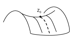
Figure 2: Schematic structure of a harmonic function in the vicinity of a stationary point $z_{0}$.

Since the function $\mbox{Re}F$ is a harmonic function of $x=\mbox{Re}z,\,y=\mbox{Im}z$, it can have only saddle points (see Fig. 2) found from the condition of stationarity $F^{\prime}(z_{0})=0$. Let us suppose that there exists only one such saddle point $z=z_{0}$, close to which we can expand $F(z)\approx F(z_{0})+C(z-z_{0})^{2}$, where $C=\frac{1}{2}F^{\prime\prime}(z_{0})$. Consider the level curves $[\mbox{Re}F](x,y)=[\mbox{Re}F](x_{0},y_{0})$, which are known either to go to infinity, or end up at a boundary of the domain of analyticity. In the vicinity of the chosen saddle-point the equation for the level curves is $\mbox{Re}[F(z)-F(z_{0})]=0$, hence

$$\mbox{Re}[|C|e^{i\theta}(z-z_{0})^{2}]=\left[(x-x_{0})^{2}(y-y_{0})^{2}\right]\cos{\theta}-2\,(x-x_{0})(y-y_{0})\sin{(\theta)}=0,$$

which describes two orthogonal straight lines passing through the saddle-point

$$y=y_{0}+\tan{\left(\frac{\pi}{4}-\frac{\theta}{2}\right)}(x-x_{0}),\quad y=y_{0}-\tan{\left(\frac{\pi}{4}+\frac{\theta}{2}\right)}(x-x_{0})$$

Figure 3: Partitioning of the $x-y$ plane in a vicinity of the stationary point $z_{0}$ into four sectors by “level curves” (solid lines). Dashed line shows the bi-sector of the negative sectors: the direction of the steepest descent contour.

partitioning the $x,y$ plane into four sectors: two “positive” ones: $\mbox{Re}F(z)>\mbox{Re}F(z_{0})$, and two “negative” ones $\mbox{Re}F(z)<\mbox{Re}F(z_{0})$, see Fig. 3. If the “edge points” of the integration contour $\Gamma$ (denoted $z_{1}$ and $z_{2}$) both belong to the same sector, and $\mbox{Re}F(z_{1})\neq\mbox{Re}F(z_{2})$, one always can deform the contour in such a way that $\mbox{Re}F(z)$ is monotonically increasing along the contour. Then obviously the main contribution to the integral comes from the vicinity of the endpoint (of the largest value of $\mbox{Re}F(z)$). Essentially the same situation happens when $z_{1}$ belongs to a negative (positive) sector, and $z_{2}$ is in a positive (resp., negative) sector. And only if the two endpoints belong to two different negative sectors, we can deform the contour in such a way, that $\mbox{Re}F(z)$ has its maximum along the contour at $z=z_{0}$, and decays away from this point. Moreover, it is easy to understand that the fastest decay away from $z_{0}$ will occur along the bi-sector of the negative sectors, i.e. along the line $y-y_{0}=\tan{\frac{\pi-\theta}{2}}(x-x_{0})$. Approximating the integration contour in the vicinity of $z_{0}$ as this bi-sector, i.e. by $z=z_{0}+(x-x_{0})\frac{e^{-i\frac{\pi-\theta}{2}}}{\sin{(\theta/2)}}$, we get the leading term of the large-$N$ asymptotics for the original integral by extending the limits of integration in the variable $\tilde{x}=x-x_{0}$ from $-\infty$ to $\infty$:

$$\int_{\Gamma}\phi(z)e^{NF(z)}dz\approx\phi(z_{0})e^{NF(z_{0})}\frac{e^{-i\frac{\pi-\theta}{2}}}{\sin{(\theta/2)}}\int_{-\infty}^{\infty}d\tilde{x}e^{-N|C|\tilde{x}^{2}}{\sin^{2}{\theta/2}}$$

$$=\phi(z_{0})\sqrt{\frac{2\pi}{N|F^{\prime\prime}(z_{0})|}}\exp{\{NF(z_{0})+\frac{i}{2}(\pi-Arg[F^{\prime\prime}(z_{0})/2)])\}}.$$ (115)

It is not difficult to make our informal consideration rigorous, and to calculate systematic corrections to the leading-order result, as well as to consider the case of several isolated saddle-points, the case of a saddle-point coinciding with an end of the contour, etc., see [7] for more detail.

After this long exposition of the method we proceed by applying it to our integral, Eq.(113). The saddle-point equation and its solution in that case amount to:

$$F^{\prime}(q)=\frac{1}{q}-q+ix=0,\quad q=q_{\pm}=\frac{1}{2}\left(ix\pm\sqrt{4-x^{2}}\right).$$

It is immediately clear that we have essentially three different cases: a) $|x|<2$ (b) $|x|>2$ and (c) $|x|=2$.

1. $|x|<2$. In this case we can introduce $x=2\cos{\phi},\,\,0<\phi<\pi$, so that $q_{\pm}=i\cos{\phi}\pm\sin{\phi}$, or $q_{+}=e^{-i(\phi-\pi/2)},\,q_{-}=e^{i(\phi+\pi/2)}$. It is easy to understand that we are interested only in $q_{+}$ (see Fig.4) and to calculate that $\mbox{Re}f(q_{+})=\frac{1}{2}\cos{(2\phi)}$. On the other hand $\mbox{Re}f(q)\to-\infty$ when either $q\to\infty$ or $q\to 0$, so that both endpoints belong to negative sectors. To understand whether they belong to the same or different sectors, we consider the values of $\mbox{Re}f(q)=\ln{R}-\frac{1}{2}(R^{2}-x^{2})$ along the real axis, $q=R$-real. As a function of the variable $R$ this expression has its maximal value $\mbox{Re}f(q=1)=-\frac{1}{2}+2\cos^{2}{\phi}$ at $q=R=1$.

   

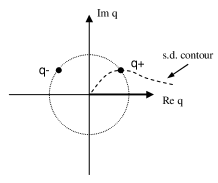
   Figure 4: Structure of the saddle-points $q_{\pm}$ and the relevant steepest descent contour for $|x|<2$.

   Noting that $\mbox{Re}f(q=1)-\mbox{Re}f(q_{+})=\cos^{2}{\phi}>0$, we conclude that the point $q=1$ belongs to a positive sector, and therefore the existence of this positive sector makes the endpoints $q=0$ and $q=\infty$ belonging to two different negative sectors, as required by the saddle-point method. Calculating

   $$f^{\prime\prime}(q_{+})=-\left(1+\frac{1}{q^{2}_{+}}\right)=2i\sin{\phi}e^{i\phi}$$

   we see that $|C|=\sin{\phi},\,\theta=\phi+\pi/2$, and further

   $$f^{\prime\prime}(q_{+})=\frac{1}{2}\cos{(2\phi)}+i\left[\frac{1}{2}\sin{(2\phi)}-\phi+\pi/2\right].$$

   Now we have all the ingredients to enter in Eq.(5.2), and can find the leading order contribution to $I_{N+n}(x)$. Further using $I_{N+n}(-x)=\overline{I_{N+n}(x)}$, valid for real $x$, we obtain the required Plancherel-Rotach asymptotics of the Hermite polynomial:

   $$h_{N+n}(x)\approx N^{N+n}\sqrt{\frac{2}{\sin{\phi}}}e^{\frac{N}{2}\cos{2\phi}}\cos{\left\{(n+1/2)\phi-\pi/4+N\left(\phi-\frac{1}{2}\sin{2\phi}\right)\right\}},$$ (116)

   where $x=2\cos{\phi},\quad 0<\phi<\pi,\quad n\ll N$.

   Now we consider the opposite case:

2. $|x|>2$. It is enough to consider explicitly the case $x>2$ and parameterize $x=2\cosh{\phi},\quad 0<\phi<\infty$. The saddle points in this case are purely imaginary:

   $$q_{\pm}=\frac{i}{2}(2\cosh{\phi}\pm 2\sinh{\phi})=ie^{\pm\phi}.$$ (117)

   One possible contour of the constant phase passing through both points is just the imaginary axis $q=iy$, where $\mbox{Im}f(q)=\pi/2$ and $\mbox{Re}f(q)=\ln{y}+\frac{1}{2}(y-x)^{2}.$ Simple consideration gives that $y_{-}=e^{-\phi}$ corresponds to the maximum, and $y_{+}=e^{\phi}$ to the minimum of $\mbox{Re}f(q)$ along such a contour. It is also clear that for $q=iy_{+}$ the expression $\mbox{Re}f(q)$ has a local maximum along the path going through this point in the direction transverse to the imaginary axis. The “topography” of $\mbox{Re}f(q)$ in the vicinity of the two saddle-points is sketched in Fig. 5

   

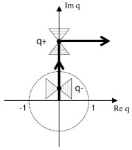
   Figure 5: The saddle-points $q_{\pm}$, the corresponding positive sectors (shaded), and the relevant steepest descent contour (bold) for $|x|>2$.

   This discussion suggests a possibility to deform the path of integration $\Gamma$ to be a contour of constant phase $\mbox{Im}f(q)$ consisting of two pieces - $\Gamma_{1}=\{q=iy,\,0\leq y\leq y_{+}\}$ and $\Gamma_{2}$ starting from $q=iy_{+}$ perpendicular to the imaginary axis and then going towards $q=\infty$. Correspondingly,

   $$I_{N+n}(x>2)=\int_{0}^{\infty}\,dq\,q^{n}\,e^{Nf(q)}=\int_{0}^{iy_{+}}\,dq\,q^{n}\,e^{Nf(q)}+\int_{\Gamma_{2}}\,dq\,q^{n}\,e^{Nf(q)}.$$ (118)

   The second integral is dominated by the vicinity of the saddle-point $q=iy_{+}$, and its evaluation by the saddle-point technique gives:

   $$\int_{\Gamma_{2}}\,dq\,q^{n}\,e^{Nf(q)}\approx\frac{1}{2}\sqrt{\frac{\pi e^{\phi}}{N\sinh{\phi}}}i^{n+N}e^{n\phi+N\left(\phi+\frac{1}{2}e^{-2\phi}\right)},$$

   where the factor $\frac{1}{2}$ arises due to the saddle-point being simultaneously the end-point of the contour. As to the first integral, it is dominated by the vicinity of $iy_{-}$, and can also be evaluated by the saddle-point method. However, it is easy to verify that when calculating $h_{N+n}(x)\propto\left[I_{N+n}(x)+(-1)^{N+n}I_{N+n}(-x)\right]$ the corresponding contribution is cancelled out. As a result, we recover the asymptotic behaviour of Hermite polynomials for $x>2$ to be given by:

   $$h_{N+n}(x=2\cosh{(2\phi)}>2)=\frac{N^{n+N}e^{-\frac{N}{2}}}{\sqrt{\sinh{\phi}}}e^{\left(n+\frac{1}{2}\right)\phi-\frac{N}{2}\left(\sinh{(2\phi)}-2\phi\right)}.$$ (119)

   Now we come to the only remaining possibility,

3. $|x|=2$. It is again enough to consider only the case $x=2$ explicitly. In fact, this is quite a special case, since for $x\to 2$ two saddle-points $q_{\pm}$ degenerate into one: $q_{+}\to q_{-}\to i$. Under such exceptional circumstances the standard saddle-point method obviously fails. Indeed, the method assumed that different saddle-points do not interfere, which means the distance $|q_{+}-q_{-}|=\sqrt{|4-x^{2}|}$ is much larger than the typical widths $W\sim\frac{1}{\sqrt{N|f^{\prime\prime}(q_{\pm})|}}$ of the regions around individual saddle-points which yield the main contribution to the integrand. Simple calculation gives $|f^{\prime\prime}(q_{\pm})|=|1+q^{-2}_{\pm}|=\sqrt{|4-x^{2}|}$, and the criterion of two separate saddle-points amounts to $|x-2|\gg N^{-2/3}$. We therefore see that in the vicinity of $x=2$ such that $|x-2|\sim N^{-2/3}$ additional care must be taken when extracting the leading order behaviour of the corresponding integral $I_{N+n}(x=2)$ as $N\to\infty$.

   To perform the corresponding calculation, we introduce a new scaling variable $\xi=N^{2/3}(2-x)$, and consider $\xi$ to be fixed and finite when $N\to\infty$. We also envisage from the discussion above that the main contribution to the integral comes from the domain around the saddle-point $q_{sp}=i$ of the widths $|q-i|\sim\sqrt{|2-x|}\sim N^{-1/3}$. The integral we are interested in is given by

   $$J_{N}(\xi) = \int_{-\infty}^{\infty}\,dq\,q^{N+n}\,e^{-\frac{N}{2}\left(q-ix\right)^{2}}$$ (120)

   $$= N^{-1/3}\int_{-\infty}^{\infty}\,dt\,\left(i+\frac{t}{N^{1/3}}\right)^{n}\,e^{N\left[\ln{(i+\frac{t}{N^{1/3}})}-\frac{1}{2}\left\{i+\frac{t}{N^{1/3}}-i\left(2-\frac{\xi}{N^{2/3}}\right)\right\}^{2}\right]}$$ (121)

   where we shifted the contour of integration from the real axis to the line $q=i+\frac{t}{N^{1/3}}\,,-\infty<t<\infty$ to ensure that it passes through the expected saddle-point $q_{sp}=i$, and also scaled the integration variable appropriately. Now we can consider $\xi,t$-finite when $N\gg 1$, and expand the integrand accordingly. A simple computation yields:

   $$J_{N\gg 1}(\xi)\approx N^{-1/3}i^{N+n}\,e^{N/2-N^{1/3}\xi}\int_{-\infty}^{\infty}\,dt\,e^{-i\xi\,t+i\frac{t^{3}}{3}}.$$ (122)

   Up to a constant factor the integral appearing in this expression is, in fact, a representation of a special function known as Airy function $Ai(\xi)$:

   $$Ai(\xi)=\frac{1}{\pi}\int_{0}^{\infty}\,dt\,\,\cos{\left(\xi\,t+\frac{t^{3}}{3}\right)}$$ (123)

   which is a solution of the second-order linear differential equation $\frac{d^{2}}{d\xi^{2}}F(\xi)-\xi\,F(\xi)=0$. A typical behaviour of such a solution is shown in Fig. 6.

   

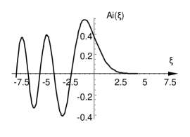
   Figure 6: The Airy function $Ai(\xi)$.

   All this results in the asymptotic behaviour of the Hermitian polynomials in the so-called “scaling vicinity” of the point $x=2$:

   $$h_{N+n}\left(x=2-\frac{\xi}{N^{2/3}}\right)\approx\frac{N^{1/6}}{\sqrt{2\pi}}N^{N+n}\,e^{N/2-N^{1/3}\xi}\,Ai(-\xi).$$ (124)

   Such scaling vicinity of $x=2$ is what gives room for a transitional regime between the oscillating asymptotics of the Hermite polynomials for $|x|<2$, see Eq.(116), and the exponential decay typical for $|x|>2$ as described in Eq.(119). Formula (124) indeed matches Eq.(116) as $\xi\to\infty$ and Eq.(119) as $\xi\to-\infty$. This statement is most easily verified by invoking the known asymptotics of the Airy function:

   $$Ai(-\xi)\approx\left\{\begin{array}[]{c}\xi^{-1/4}\pi^{-1/2}\cos{\left(-\frac{2}{3}\xi^{3/2}+\frac{\pi}{4}\right)},\quad\xi\to\infty\\ \frac{1}{\pi^{1/2}|\xi|^{1/4}}\,e^{-\frac{2}{3}|\xi|^{3/2}},\quad\xi\to-\infty\end{array}\right.$$ (125)

   and identifying $\phi=|\xi|^{1/2}N^{-1/3}\ll 1$ in the corresponding expressions.

Now we are going to apply the derived formulae for extracting the large-N behaviour of the mean eigenvalue density and the kernel as described in Eqs.(108) and(110), respectively. In fact, it is more conventional in the random matrix literature to use the mean density to be normalized to unity, rather than to $N$. Such a density will have a well-defined large-N limit which we will denote as $\rho_{\infty}(\lambda)$.

6 Scaling regimes for GUE

6.1 Bulk scaling: Wigner semicircle and Dyson kernel.

The first case to be considered is the spectral parameter $|\lambda|<2$ when we can parameterize $\lambda=2\cos{\phi}$, and exploit the Plancherel-Rotach expression (116) for the Hermite polynomials. Furthermore, denoting $\alpha=\frac{1}{2}\phi-\frac{\pi}{4}+N\left(\phi-\frac{1}{2}\sin{2\phi}\right)$, and using the identity $\cos^{2}{\alpha}-\cos{(\alpha+\phi)}\cos{(\alpha-\phi)}=\sin^{2}{\phi}$ we find that $h_{N}^{2}(\lambda)-h_{N-1}(\lambda)h_{N+1}(\lambda)\approx 2N^{2N}\sin{\phi}e^{N\cos{(2\phi)}}$. Furthermore, using for large $N$ the Stirling formula: $(N-1)!\approx\sqrt{\frac{2\pi}{N}}N^{N}e^{-N}$ and remembering that $\sin{\phi}=\frac{1}{2}\sqrt{4-\lambda^{2}}$ we arrive, after collecting all factors, to the famous Wigner semicircular law for the mean (normalized) spectral density:

$$\lim_{N\to\infty}\left[\frac{1}{N}\overline{\rho(\lambda)}\right]=\rho_{\infty}(\lambda)=\frac{1}{2\pi}\sqrt{4-\lambda^{2}},\quad|\lambda|<2.$$ (126)

We see that in the limit of large $N$ all $N$ eigenvalues of GUE matrices are concentrated in the interval $[-2,2]$, and the typical separation of two neighbouring eigenvalues close to an “internal” point $\lambda\in(-2,2)$ is $\Delta=\frac{1}{N\rho_{\infty}(\lambda)}=O(N^{-1})$, see Fig. 7. That is why the case $\lambda\in(-2,2)$ is frequently referred to as the ”bulk of the spectrum” regime.

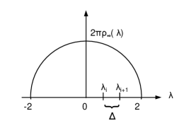
Figure 7: Wigner semicircular density. Sketch shows a typical spacing between neighbouring levels in the bulk of the spectrum.

Let us now follow the same strategy for obtaining, under the same conditions, the limiting expression for the kernel $K(\lambda,\lambda^{\prime})$ using for this goal formula (110). We have:

$$h_{N}(\lambda)h_{N-1}(\lambda^{\prime})-h_{N}(\lambda^{\prime})h_{N-1}(\lambda)$$ (127)

$$\approx 2N^{2N}\frac{1}{\sqrt{\sin{\phi}\sin{\phi^{\prime}}}}e^{\frac{N}{2}\left(\cos{(2\phi)}+\cos{(2\phi^{\prime})}\right)}\left[\cos{\alpha_{1}^{+}}\cos{\alpha_{2}^{-}}-\cos{\alpha_{1}^{-}}\cos{\alpha_{2}^{+}}\right]$$ (128)

where $\alpha^{\pm}_{1}=\pm\frac{1}{2}\phi-\frac{\pi}{4}+N\left(\phi-\frac{1}{2}\sin{2\phi}\right),\,\,\alpha^{\pm}_{2}=\pm\frac{1}{2}\phi^{\prime}-\frac{\pi}{4}+N\left(\phi^{\prime}-\frac{1}{2}\sin{2\phi^{\prime}}\right)$. The next step is to introduce $\psi=(\phi+\phi^{\prime})/2$ and $\Omega=(\phi-\phi^{\prime})/2$, and to consider the parameter $\Omega$ to be of the order of $O(N^{-1})$ when taking the limit. This choice ensures that the distance $\lambda-\lambda^{\prime}=2[\cos{\phi}-\cos{\phi^{\prime}}]\approx 4\Omega\sin{\psi}\approx 4\Omega\pi\rho_{\infty}(\lambda)$ is of the order of the mean eigenvalue separation $\Delta$ - the typical scale for the correlations between the eigenvalues in the bulk of the spectrum- and thus must be reflected in the structure of the kernel. To this end we denote $\Omega=\omega/N$, and keep in the expressions for $\alpha^{\pm}_{1,2}$ terms up to the order $O(1)$, i.e. writing $\alpha^{\pm}_{1,2}=N\beta+\left[\pm\frac{1}{2}\psi-\frac{\pi}{4}\pm 2\omega\sin^{2}{\psi}\right]$, where $\beta=\left(\psi-\frac{1}{2}\sin{2\psi}\right)$. With the same precision:

$$\cos{\alpha_{1}^{+}}\cos{\alpha_{2}^{-}}-\cos{\alpha_{1}^{-}}\cos{\alpha_{2}^{+}}\approx\sin{\psi}\sin{\left(4\omega\sin^{2}{\psi}\right)}\approx\sin{\psi}\sin{\left[\pi\rho_{\infty}(\lambda)N(\lambda_{1}-\lambda_{2})\right]}$$

and $\cos{2\phi_{1}}+\cos{2\phi_{2}}\approx 2\left(\frac{\lambda^{2}}{2}-1\right)$ substituting all these factors back into Eq.(127), we get

$$h_{N}(\lambda)h_{N-1}(\lambda^{\prime})-h_{N}(\lambda^{\prime})h_{N-1}(\lambda)\approx 2N^{2N}e^{2N\left(\frac{\lambda^{2}}{2}-1\right)}\sin{\left[\pi\rho_{\infty}(\lambda)N(\lambda-\lambda^{\prime})\right]}.$$ (129)

Now, taking into account the normalization factors in $\tilde{h}_{N}(\lambda)$ and $\tilde{h}_{N-1}(\lambda),$ see Eq.(92), using again the Stirling formula and invoking Eq.(81) we arrive at the following asymptotic expression for the kernel, Eq.(110):

$$\lim_{N\to\infty}\left[\frac{K_{N}(\lambda,\lambda^{\prime})}{K_{N}(\lambda,\lambda)}\right]=K_{\infty}\left[N\rho_{\infty}(\lambda)(\lambda-\lambda^{\prime})\right],\quad K_{\infty}(r)=\frac{\sin{\pi r}}{\pi r}$$ (130)

where $K_{\infty}(r)$ is the famous Dyson scaling form for the kernel. The formula is valid as long as both $\lambda$ and $\lambda^{\prime}$ are within the range $(-2,2)$, and $\lambda-\lambda^{\prime}=O(N^{-1})$. Such choice of the parameters is frequently referred to as the “bulk scaling” limit.

Having at our disposal the limiting form of both mean eigenvalue density and the two-point kernel we can analyse such important statistical characteristics of the spectra as e.g. the “number variance”, see Eq.(48), for an interval of the length $L$ comparable with the mean spacing close to the origin $\Delta=[N\rho_{\infty}(0)]^{-1}$. Under such a condition we can legitimately employ the scaling form Eq.(130) of the kernel when substituting it into formula (82) for the cluster function $Y_{2}(\lambda,\lambda^{\prime})$. In this way we arrive at

$$\Sigma_{2}(L)=N\int_{-L/2}^{L/2}\rho_{\infty}(\lambda)d\lambda-N^{2}\int_{-L/2}^{L/2}d\lambda\,\int_{-L/2}^{L/2}d\lambda^{\prime}\rho_{\infty}(\lambda)\rho_{\infty}(\lambda^{\prime})K^{2}_{\infty}\left[N\rho_{\infty}(\lambda)(\lambda-\lambda^{\prime})\right]$$

$$=s-\int_{-s/2}^{s/2}du\,\int_{-s/2}^{s/2}\,du^{\prime}K^{2}_{\infty}\left[(u-u^{\prime})\right].$$ (131)

Here we used the fact that with the same precision we can put $\rho_{\infty}(\lambda)\approx\rho_{\infty}(\lambda^{\prime})\approx\rho_{\infty}(0)$ in the above expression, and introduced the natural scaling variables: $u=\lambda/\Delta,\,u=\lambda^{\prime}/\Delta$ as well as the scaled length of the interval $s=L/\Delta$ (cf. a similar procedure for Poissonian sequences after Eq.(57)). To simplify this expression further we introduce $u_{+}=(u+u^{\prime})/2,\,r=u-u^{\prime}$ as integration variables, and use that, in fact $K_{\infty}(r)\equiv K_{\infty}(|r|)$. The number variance takes the final form:

$$\Sigma_{2}(s)=s-\int_{-s}^{s}\,dr\,\int_{-\frac{s}{2}+\frac{|r|}{2}}^{\frac{s}{2}-\frac{|r|}{2}}\,du_{+}K^{2}_{\infty}(|r|)=s-2\int_{0}^{s}\,dr\,(s-r)\left[\frac{\sin{\pi r}}{\pi r}\right]^{2}.$$ (132)

In fact, we are mainly interested in the large-$s$ behaviour of this expression. To extract it, we use the identity: $2\int_{0}^{\infty}\,dr\,\left[\frac{\sin{\pi r}}{\pi r}\right]^{2}=\frac{2}{\pi}\int_{0}^{\infty}\,dx\,\left[\frac{\sin{x}}{x}\right]^{2}=1$, and rewrite the above expression as

$$\Sigma_{2}(s)=\frac{2s}{\pi}\int_{\pi s}^{\infty}\,dx\,\frac{\sin^{2}{x}}{x^{2}}+\frac{1}{\pi^{2}}\int_{0}^{2\pi s}\frac{1-\cos{x}}{x}\,dx.$$ (133)

The second integral obviously grows logarithmically with $s$ and dominates at large $s$. A more accurate evaluation gives the asymptotic formula:

$$\Sigma_{2}(s\gg 1)=\frac{1}{\pi^{2}}\left[\ln{2\pi s}+\gamma+1\right]+O(1/s).$$ (134)

where $\gamma=0.5772...$ is Euler’s constant. This is much slower than the linear growth $\Sigma_{2}(s\gg 1)=s$ typical for uncorrelated (Poissonian) sequence, see Fig. 8. The explanation of the slow growth is that the sequence of eigenvalues is, in fact, quite ordered, with quite regular spacings of the order of $\Delta$, and therefore the number of points in the interval does not fluctuate as much as it does for uncorrelated sequence.

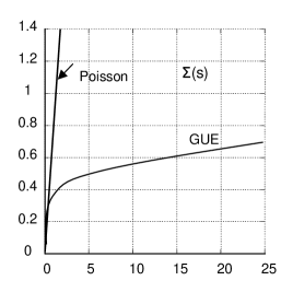
Figure 8: The logarithmic growth of the number variance $\Sigma(s)$ for large GUE matrices versus linear growth for uncorrelated (Poissonian) spectrum.

As to another important and frequently used statistical characteristic of spectral sequences - the “hole probability”- its calculation amounts to investigating the asymptotics of the Fredholm determinant of the kernel $K_{N\to\infty}$, see Eq.(88). This is a very difficult mathematical problem, and the most elegant solution uses an advanced mathematical technique known as the Riemann-Hilbert method[3]. Let us just quote the result:

$$A(s\gg 1)\propto\frac{1}{s^{1/4}}e^{-\frac{\pi^{2}}{8}s^{2}}.$$ (135)

This Gaussian decay should be again contrasted with a much slower exponential decay typical for uncorrelated sequences as indeed in full correspondence with a “quasiregular” structure of the random matrix spectrum.

6.2 Edge scaling regime and Airy kernel

As we already know, in the vicinity of the “spectral edge” $x=2$ (and its counterpart $x=-2$) the Plancherel-Rotach asymptotics of the Hermitian polynomials changes, and is basically given by the Airy function, see Eq.(124). This certainly results in essential modifications of the large$-N$ behaviour of the mean eigenvalue density and of the two-point kernel as long as $|\lambda-2|\sim N^{-2/3}$. To extract the explicit formulae for this so-called “edge scaling” limit one may try the same strategy as in the bulk. However, one immediately discovers that simple substitution of Eq.(124) into formula (109) for the mean density yields zero. A possible way out may be to calculate the next-to-leading order corrections to the asymptotics of $h_{N}(x)$, but we will rather follow a slightly different (and more direct) route and consider the integral representation for the main combination of interest:

$${\cal D}_{N}(\lambda)=h^{2}_{N}(\lambda)-h_{N-1}(\lambda)h_{N+1}(\lambda)=\frac{(-1)^{N}}{2\pi}N^{2N}\,\int_{-\infty}^{\infty}\,dq_{1}\int_{-\infty}^{\infty}\,dq_{2}\frac{q_{1}-q_{2}}{q_{1}}e^{N\left[f(q_{1})+f(q_{2})\right]}$$ (136)

where we exploited Eq.(111,113), and defined, as before, $f(q)=\ln{q}-\frac{1}{2}\left(q-i\lambda\right)^{2}$. To evaluate this integral in the edge scaling limit, we follow a familiar procedure: introduce the scaling variable $\xi=N^{2/3}(\lambda-2)$, shift the contours of integration from the real axis to the lines $q_{1,2}=i+\frac{t_{1,2}}{N^{1/3}}\,,-\infty<t_{1,2}<\infty$, consider $\xi,\,t_{1,2}$ to be fixed and finite when $N\to\infty$, and expand the integrand accordingly around the saddle-points $t_{1,2}=0$. Simple calculation yields, in complete analogy with Eq.(122), the expression:

$${\cal D}_{N}(\xi)\approx\frac{N^{2N}}{2\pi}N^{-1/3}\,e^{N+2N^{1/3}\xi}$$

$$\times\left\{\int_{\Gamma}\,dt_{1}\,e^{i\xi\,t_{1}+i\frac{t_{1}^{3}}{3}}\int_{\Gamma}\,dt_{2}\,t_{2}^{2}\,e^{i\xi\,t_{2}+i\frac{t_{2}^{3}}{3}}-\int_{\Gamma}\,dt_{1}\,t_{1}\,e^{i\xi\,t_{1}+i\frac{t_{1}^{3}}{3}}\int_{\Gamma}\,dt_{2}\,t_{2}\,e^{i\xi\,t_{2}+i\frac{t_{2}^{3}}{3}}\right\}.$$ (137)

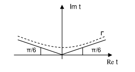
Figure 9: The contour of integration $\Gamma$ in the definition of the Airy function.

The only essential difference from Eq.(122) which deserves mentioning is the choice of the integration contour $\Gamma$ which ensures the existence of all the integrals involved. Obviously, one can not simply take $\Gamma=(-\infty,\infty)$, but a more detailed investigation shows that the correct contour must be chosen in such a way as to be asymptotically tangent to the line $\mbox{Arg}{(t)}=5\pi/6$ for $\mbox{Re}\,t\to-\infty$, and asymptotically tangent to $\mbox{Arg}{(t)}=\pi/6$ for $\mbox{Re}\,t\to\infty$, see Fig.9. It is then evident, that

$$Ai(\xi)=\frac{1}{\pi}\int_{\Gamma}\,dt\,e^{i\xi\,t+i\frac{t^{3}}{3}},\,\,-iAi^{\prime}(\xi)=\frac{1}{\pi}\int_{\Gamma}\,dt\,t\,e^{i\xi\,t+i\frac{t^{3}}{3}},\,\,-Ai^{\prime\prime}(\xi)=\frac{1}{\pi}\int_{\Gamma}\,dt\,t^{2}\,e^{i\xi\,t+i\frac{t^{3}}{3}}$$

and collecting all factors we find the expression of the mean eigenvalue density close to the “spectral edge”:

$$\overline{\rho}(\lambda=2+\xi\,N^{-2/3})\propto\rho_{e}(\xi)=Ai^{\prime}(\xi)^{2}-Ai^{\prime\prime}(\xi)Ai(\xi).$$ (138)

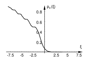
Figure 10: Behaviour of the spectral density close to the spectral edge.

For $\xi<0$ the function shows noticeable oscillations , see Fig.10, with neighbouring maxima separated by distance of the order of $\lambda_{i}-\lambda_{i-1}\propto\Delta_{edge}=\sim N^{-1/3}$ and reflecting typical positions of individual eigenvalues close to the “spectral edge”. In contrast, for $\xi>0$ the mean density decays extremely fast, reflecting the typical absence of the eigenvalues beyond the spectral edge.

A very similar calculation shows that under the same conditions the kernel $K_{N}(\lambda,\lambda^{\prime})$ assumes the form:

$$K(\xi_{1},\xi_{2})=\frac{Ai(\xi_{1})Ai^{\prime}(\xi_{2})-Ai(\xi_{2})Ai^{\prime}(\xi_{1})}{\xi_{1}-\xi_{2}}$$ (139)

known as the Airy kernel, see [8].

7 Orthogonal polynomials versus characteristic polynomials

Our efforts in studying Hermite polynomials in detail were amply rewarded by the provided possibility to arrive at the bulk and edge scaling forms for the matrix kernel in the corresponding large-N limits. It is those forms which turn out to be universal, which means independent of the particular detail of the random matrix probability distribution, provided size of the corresponding matrices is large enough. This is why one can hope that the Dyson kernel would be relevant to many applications, including properties of the Riemann $\zeta$-function. An important issue for many years was to prove the universality for unitary-invariant ensembles which was finally achieved, first in [10].

In fact, quite a few basic properties of the Hermite polynomials are shared also by any other set of orthogonal polynomials $\pi_{k}(x)$. Among those worth of particular mentioning is the Christoffel-Darboux formula for the combination entering the two-point kernel Eq.(73), (cf. Eq.(103)):

$$\sum_{k=0}^{n-1}\pi_{k}(x)\pi_{k}(y)=b_{n}\frac{\pi_{n-1}(y)\pi_{n}(x)-\pi_{n-1}(x)\pi_{n}(y)}{x-y},$$ (140)

where $b_{n}$ are some constants. So the problem of the universality of the kernel (and hence, of the n-point correlation functions) amounts to finding the appropriate large-$N$ scaling limit for the right-hand side of Eq.(140) (in the “bulk” of the spectrum, or close to the spectral “edge”).

The main dissatisfaction is that explicit formulas for orthogonal polynomials (most important, an integral representation similar to Eq.(106)) are not available for general weight functions $dw(\lambda)=e^{-Q(\lambda)}d\lambda$. For this reason we have to devise alternative tools of constructing the orthogonal polynomials and extracting their asymptotics. Any detailed discussion of the relevant technique goes far beyond the modest goals of the present set of lectures. Nevertheless, some hints towards the essence of the powerful methods employed for that goal will be given after a digression.

Namely, I find it instructive to discuss first a question which seems to be quite unrelated,- the statistical properties of the characteristic polynomials

$$Z_{N}(\mu)=\det\left(\mu{\bf 1}_{N}-\hat{H}\right)=\prod_{i=1}^{N}(\mu-\lambda_{i})$$ (141)

for any Hermitian matrix ensemble with invariant JPDF ${\cal P}(\hat{H})\propto\exp\{-N\mbox{Tr}Q(\hat{H})\}$. Such objects are very interesting on their own for many reasons. Moments of characteristic polynomials for various types of random matrices were much studied recently, in particular due to an attractive possibility to use them, in a very natural way, for characterizing “universal” features of the Riemann $\zeta$-function along the critical line, see the pioneering paper[11] and the lectures by Jon Keating in this volume. The same moments also have various interesting combinatorial interpretations, see e.g. [12, 13], and are important in applications to physics, as I will elucidate later on.

On the other hand, addressing those moments will allow us to arrive at the most natural way of constructing polynomials orthogonal with respect to an arbitrary weight $dw(\lambda)=e^{-Q(\lambda)}d\lambda$. To understand this, we start with considering the lowest moment, which is just the expectation value of the characteristic polynomial:

$$E\left[Z_{N}(\mu)\right]=\int_{-\infty}^{\infty}dw(\lambda_{1})\ldots\int_{-\infty}^{\infty}dw(\lambda_{N})\prod_{i<j}^{N}(\lambda_{i}-\lambda_{j})^{2}\,\prod_{i=1}^{N}(\mu-\lambda_{i})$$ (142)

We first notice that

$$\prod_{i<j}^{N}(\lambda_{i}-\lambda_{j})\,\prod_{i=1}^{N}(\mu-\lambda_{i})\propto\det{\left(\begin{array}[]{cccc}1&\ldots&1&1\\ \lambda_{1}&\ldots&\lambda_{N}&\mu\\ .&.&.&.\\ .&.&.&.\\ .&.&.&.\\ \lambda^{N-1}_{1}&\ldots&\lambda^{N-1}_{N}&\mu^{N-1}\\ \lambda^{N}_{1}&\ldots&\lambda^{N}_{N}&\mu^{N}\end{array}\right)}$$ (143)

Indeed, the right-hand side is obviously a polynomial of degree $N$ in the variable $\mu$, with roots at $\mu=\mu_{1},\mu_{2},\ldots,\mu_{N}$. Therefore it must be of the form $C\times\prod_{i=1}^{N}(\mu-\lambda_{i})$, with prefactor $C$ being a function of $\lambda_{1},...,\lambda_{N}$. The value of such a prefactor can be easily established by comparing both sides as $\mu\to\infty$: the left-hand side behaves as $C\,\mu^{N}$, whereas expanding the determinant with respect to the last column and using the expression for the van der Monde determinant, Eq.(66), we see that the right-hand side grows as $\mu^{N}\prod_{i<j}^{N}(\lambda_{i}-\lambda_{j})$.

Exploiting Eq.(143) allows us to rewrite the expectation value for the characteristic polynomial as

$$E\left[Z_{N}(\mu)\right]\propto\int_{-\infty}^{\infty}\prod_{i=1}^{N}dw(\lambda_{i})\det{\left(\begin{array}[]{ccc}1&\ldots&1\\ \lambda_{1}&\ldots&\lambda_{N}\\ .&.&.\\ .&.&.\\ .&.&.\\ \lambda^{N-1}_{1}&\ldots&\lambda^{N-1}_{N}\end{array}\right)}\det{\left(\begin{array}[]{cccc}1&\ldots&1&1\\ \lambda_{1}&\ldots&\lambda_{N}&\mu\\ .&.&.&.\\ .&.&.&.\\ .&.&.&.\\ \lambda^{N}_{1}&\ldots&\lambda^{N}_{N}&\mu^{N}\end{array}\right)},$$ (144)

which can be further written down as the standard sum over all permutations $P_{\sigma}=(\sigma_{1},\,\ldots,\,\sigma_{N})$ of the index set $(1,2,...,N)$:

$$E\left[Z_{N}(\mu)\right]\propto\sum_{P_{\sigma}}(-1)^{|P_{\sigma}|}\int_{-\infty}^{\infty}\prod_{i=1}^{N}dw(\lambda_{i})\lambda^{0}_{\sigma_{1}}\ldots\lambda^{N-1}_{\sigma_{N}}\det{\left(\begin{array}[]{cccc}1&\ldots&1&1\\ \lambda_{1}&\ldots&\lambda_{N}&\mu\\ .&.&.&.\\ .&.&.&.\\ .&.&.&.\\ \lambda^{N}_{1}&\ldots&\lambda^{N}&\mu^{N}\end{array}\right)},$$ (145)

where $|P_{\sigma}|=0(1)$ for even(odd) permutations. The symmetry of the remaining determinant with respect to permutation of its columns ensures that every term in the sum above yields exactly the same contribution, and it is enough to consider only the first term with $P_{\sigma}=(1,2,...,N)$, and multiply the result with $N!$. For such a choice, the product of factors $\lambda^{0}_{1}\ldots\lambda^{N-1}_{N}$ can be “absorbed” in the determinant by multiplying the $j-$th column of the latter with the factor $\lambda^{j-1}_{j}$, for all $j=1,\ldots,N$. This gives

$$E\left[Z_{N}(\mu)\right]\propto\int_{-\infty}^{\infty}\prod_{i=1}^{N}dw(\lambda_{i})\det{\left(\begin{array}[]{ccccc}1&\lambda_{2}&\ldots&\lambda_{N}^{N-1}&1\\ \lambda_{1}&\lambda_{2}^{2}&\ldots&\lambda^{N}_{N}&\mu\\ .&.&.&.&\\ .&.&.&.&\\ .&.&.&.&\\ \lambda^{N-1}_{1}&\lambda^{N}_{2}&\ldots&\lambda^{2N-2}_{N}&\mu^{N-1}\\ \lambda^{N}_{1}&\lambda^{N+1}_{2}&\ldots&\lambda^{2N-1}_{N}&\mu^{N}\end{array}\right)}.$$ (146)

The integral in the right-hand side is obviously a polynomial of degree $N$ in $\mu$, which we denote $D_{N}(\mu)$ and write in the final form as

$$D_{N}(\mu)=\det{\left(\begin{array}[]{ccccc}\int_{-\infty}^{\infty}dw(\lambda)&\int_{-\infty}^{\infty}dw(\lambda)\lambda&\ldots&\int_{-\infty}^{\infty}dw(\lambda)\lambda^{N-1}&1\\ \int_{-\infty}^{\infty}dw(\lambda)\lambda&\int_{-\infty}^{\infty}dw(\lambda)\lambda^{2}&\ldots&\int_{-\infty}^{\infty}dw(\lambda)\lambda^{N}&\mu\\ .&.&.&.&\\ .&.&.&.&\\ .&.&.&.&\\ \int_{-\infty}^{\infty}dw(\lambda)\lambda^{N-1}&\int_{-\infty}^{\infty}dw(\lambda)\lambda^{N}&\ldots&\int_{-\infty}^{\infty}dw(\lambda)\lambda^{2N-2}&\mu^{N-1}\\ \int_{-\infty}^{\infty}dw(\lambda)\lambda^{N}&\int_{-\infty}^{\infty}dw(\lambda)\lambda^{N+1}&\ldots&\int_{-\infty}^{\infty}dw(\lambda)\lambda^{2N-1}&\mu^{N}\end{array}\right)}.$$ (147)

The last form makes evident the following property. Multiply the right-hand side with $dw(\mu)\mu^{p}$ and integrate over $\mu$. By linearity, the factor and the integration can be “absorbed” in the last column of the determinant. For $p=0,1,\ldots,N-1$ this last column will be identical to one of preceding columns, making the whole determinant vanishing, so that

$$\int_{-\infty}^{\infty}dw(\mu)\mu^{p}D_{N}(\mu)=0,\quad p=0,1,\ldots,N-1.$$ (148)

Moreover, it is easy to satisfy oneself that the polynomial $D_{N}(\mu)$ can be written as $D_{N}(\mu)=D_{N-1}\mu^{N}+\ldots$, where the leading coefficient $D_{N-1}=\det{\left(\int_{-\infty}^{\infty}dw(\lambda)\lambda^{i+j}\right)_{i,j=0}^{N}}$ is necessarily positive: $D_{n-1}>0$. The last fact immediately follows from the positivity of the quadratic form:

$$G(x_{1},\ldots,x_{N})=\int_{-\infty}^{\infty}dw(\lambda)\left(\sum_{i=1}^{N}\,x_{i}\lambda^{i}\right)^{2}=\sum_{i,j}^{N}x_{i}x_{j}\int_{-\infty}^{\infty}dw(\lambda)\lambda^{i+j}$$

Finally, notice that

$$\int_{-\infty}^{\infty}dw(\mu)D_{N}^{2}(\mu)=\int_{-\infty}^{\infty}dw(\mu)D_{N}(\mu)\left[D_{N-1}\mu^{N}+lower\,\,powers\right]$$ (149)

$$=D_{N-1}\int_{-\infty}^{\infty}dw(\mu)D_{N}(\mu)\mu^{N}=D_{N-1}D_{N}$$

where we first exploited Eq.(148) and at the last stage Eq.(147). Combining all these facts together we thus proved that the polynomials $\pi_{N}(\lambda)=\frac{1}{\sqrt{D_{N-1}D_{N}}}D(\lambda)$ form the orthogonal (and normalized to unity) set with respect to the given measure $dw(\lambda)$. Moreover, our discussion makes it immediately clear that the expectation value of the characteristic polynomial $Z_{N}(\mu)$ for any given random matrix ensemble is nothing else, but just the corresponding monic orthogonal polynomial:

$$E\left[Z_{N}(\mu)\right]=\pi^{(m)}_{N}(\mu),$$ (150)

whose leading coefficient is unity. Leaving aside the modern random matrix interpretation the combination of the right hand sides of the formulas Eq.(150) and Eq.(142) goes back, according to [6], to Heine-Borel work of 1878, and as such is completely classical.

The random matrix interpretation is however quite instructive, since it suggests to consider also higher moments of the characteristic polynomials, and even more general objects like the correlation functions

$${\cal C}_{k}(\mu_{1},\mu_{2},\ldots,\mu_{k})=E\left[Z_{N}(\mu_{1})Z_{N}(\mu_{2})\ldots Z_{N}(\mu_{k})\right].$$ (151)

Let us start with considering

$${\cal C}_{2}(\mu_{1},\mu_{2})=\int_{-\infty}^{\infty}dw(\lambda_{1})\ldots\int_{-\infty}^{\infty}dw(\lambda_{N})\prod_{i<j}^{N}(\lambda_{i}-\lambda_{j})^{2}\,\prod_{i=1}^{N}(\mu_{1}-\lambda_{i})\prod_{i=1}^{N}(\mu_{2}-\lambda_{i}).$$ (152)

Using the notation $\Delta_{N}(\lambda_{1},\ldots,\lambda_{N})$ for the van der Monde determinant, see Eq.(66), we further notice that

$$\Delta_{N+2}(\lambda_{1},\ldots,\lambda_{N},\mu_{1},\mu_{2})=\Delta_{N}(\lambda_{1},\ldots,\lambda_{N})\times(\mu_{1}-\mu_{2})\prod_{i=1}^{N}(\mu_{1}-\lambda_{i})\prod_{i=1}^{N}(\mu_{2}-\lambda_{i}),$$

which allows us to rewrite the correlation function as

$${\cal C}_{2}(\mu_{1},\mu_{2})=\frac{1}{(\mu_{1}-\mu_{2})}\int_{-\infty}^{\infty}\prod^{N}_{i=1}dw(\lambda_{i})\,\Delta_{N}(\lambda_{1},\ldots,\lambda_{N})\Delta_{N+2}(\lambda_{1},\ldots,\lambda_{N},\mu_{1},\mu_{2}).$$

Now we replace each entry $\lambda_{i}^{j}$ in both van der Monde determinant factors with the orthogonal polynomial $\pi_{j}(\lambda_{i})$ (cf. eq.(67)), and further expand the first factor as a sum over permutations: $\Delta_{N}(\lambda_{1},\ldots,\lambda_{N})\propto\sum_{P}(-1)^{|P|}\pi_{0}(\lambda_{\sigma_{1}})\ldots\pi_{N-1}(\lambda_{\sigma_{N}})$. Further using permutational symmetry of the second determinant, we again see that every term yields after integration the same contribution. Up to a proportionality factor we can therefore rewrite the correlation function as

$${\cal C}_{2}(\mu_{1},\mu_{2}) = \frac{1}{(\mu_{1}-\mu_{2})}\int_{-\infty}^{\infty}\prod^{N}_{i=1}dw(\lambda_{i})\,\pi_{0}(\lambda_{1})\ldots\pi_{N-1}(\lambda_{N})$$ (153)

$$\times \det{\left(\begin{array}[]{ccccc}\pi_{0}(\lambda_{1})&\pi_{0}(\lambda_{2})&\ldots&\pi_{0}(\mu_{1})&\pi_{0}(\mu_{2})\\ \pi_{1}(\lambda_{1})&\pi_{1}(\lambda_{2})&\ldots&\pi_{1}(\mu_{1})&\pi_{1}(\mu_{2})\\ .&.&.&.&\\ .&.&.&.&\\ .&.&.&.&\\ \pi_{N}(\lambda_{1})&\pi_{N}(\lambda_{2})&\ldots&\pi_{N}(\mu_{1})&\pi_{N}(\mu_{2})\\ \pi_{N+1}(\lambda_{1})&\pi_{N+1}(\lambda_{2})&\ldots&\pi_{N+1}(\mu_{1})&\pi_{N+1}(\mu_{2})\end{array}\right)}.$$ (161)

At the next step we absorb the factors $\pi_{0}(\lambda_{1}),\dots,\pi_{N-1}(\lambda_{N})$ inside the determinant by multiplying the first column with $\pi_{0}(\lambda_{1})$,…, the $N-th$ column with $\pi_{N-1}(\lambda_{N})$, and leaving the last two columns intact. By linearity, we can also absorb the product of the integrals inside the determinant by integrating the first column over $\lambda_{1}$,…, and $N-th$ column over $\lambda_{N}$. Due to the orthogonality, the first $N$ columns of the resulting determinant after integration contain zero components off-diagonal, whereas the entries on the main diagonal are equal to the normalization constants $c_{k}=\int_{-\infty}^{\infty}dw(\lambda)\,\pi^{2}_{k}(\lambda),\,\,k=0,\dots,N$. Therefore, the resulting determinant is easy to calculate and, up to a multiplicative constant we arrive to the following simple formula:

$${\cal C}_{2}(\mu_{1},\mu_{2})\propto\frac{1}{(\mu_{1}-\mu_{2})}\det{\left(\begin{array}[]{cc}\pi_{N}(\mu_{1})&\pi_{N}(\mu_{2})\\ \pi_{N+1}(\mu_{1})&\pi_{N+1}(\mu_{2})\end{array}\right)}.$$ (162)

In particular, for the second moment of the characteristic polynomial we have the expression

$$E[Z^{2}(\mu)]=\lim_{\mu_{1}\to\mu_{2}=\mu}{\cal C}_{2}(\mu_{1},\mu_{2})\propto\det{\left(\begin{array}[]{cc}\pi_{N}(\mu)&\pi^{\prime}_{N}(\mu)\\ \pi_{N+1}(\mu)&\pi^{\prime}_{N+1}(\mu)\end{array}\right)}.$$ (163)

This procedure can be very straightforwardly extended to higher order correlation functions[14, 16], and higher order moments[15] of the characteristic polynomials. The general structure is always the same, and is given in the form of a determinant whose entries are orthogonal polynomials of increasing order.

One more observation deserving mentioning here is that the structure of the two-point correlation function of characteristic polynomials is identical to that of the Christoffel-Darboux, which is the main building block of the kernel function, Eq.(73). Moreover, comparing the above formula (163) for the gaussian case with expressions (108,107), one notices a great degree in similarity between the structure of mean eigenvalue density and that for the second moment of the characteristic polynomial. All these similarities are not accidental, and there exists a general relation between the two types of quantities as I proceed to demonstrate on the simplest example. For this we recall that the mean eigenvalue density $\overline{\rho_{N}(\lambda)}$ is just the one-point correlation function, see Eq.(42), and according to Eq.(39) and Eq.(38) can be written as

$${\cal R}_{1}(\lambda) = N\int\,{\cal P}(\lambda,\lambda_{2},\ldots,\lambda_{N})\,\,d\lambda_{2}\,\ldots\,\lambda_{N}$$ (164)

$$\propto e^{-Q(\lambda)}\int d\lambda_{2}\,\ldots\,\lambda_{N}e^{-\sum_{i=2}^{N}Q(\lambda_{i})}\prod_{i=2}^{N}(\lambda-\lambda_{i})^{2}\prod_{2\leq i<j\leq N}\left(\lambda_{i}-\lambda_{j}\right)^{2}.$$

It is immediately evident after simple renumbering $(\lambda_{2},\ldots,\lambda_{N})\to(\lambda_{1},\ldots,\lambda_{N-1})$ that the integral in the second line allows a clear interpretation as the second moment of the characteristic polynomial $E[Z^{2}_{N-1}(\lambda)]$ of a random matrix $H_{N-1}$ distributed according to the same joint probability density function ${\cal P}\left(H_{N-1}\right)d\hat{H}_{N-1},$ but of reduced size $N-1$, see Eq.(142) for comparison. We therefore have a general relation between the mean eigenvalue density and the second moment of the characteristic polynomial of the reduced-size matrix:

$$\overline{\rho_{N}(\lambda)}\propto e^{-Q(\lambda)}\overline{\left[\det{\left(\lambda{\bf 1}_{N}-\hat{H}_{N-1}\right)}\right]^{2}}$$ (165)

which explains the observed similarity. This type of relations, and their natural generalizations to higher-order correlation functions hold for general invariant ensembles and were found helpful in several applications; e.g. for the so-called “chiral” ensembles (notion of such ensembles is shortly discussed in the very end of these notes) in [18], for non-Hermitian matrices with complex eigenvalues see examples and further references in [19]); for real symmetric matrices see the recent paper[20].

Now let us discuss another important class of correlation functions involving characteristic polynomials, - namely one combining both positive and negative moments, the simplest example being the expectation value of the ratio:

$${\cal K}_{N}(\mu,\nu)=E\left[\frac{Z_{N}(\mu)}{Z_{N}(\nu)}\right].$$ (166)

For such an object to be well-defined it is necessary to regularize the characteristic polynomial in the denominator $Z_{N}(\nu)=\det\left(\nu{\bf 1}_{N}-\hat{H}\right)$ by considering the complex-valued spectral parameter $\nu$ such that $\mbox{Im}\nu\neq 0$. Further generalizations include more than one polynomial in numerator and/or denominator.

Such objects turned out to be indispensable tools in applications of random matrices to physical problems. In fact, in all applications a very fundamental role is played by the resolvent matrix $(\mu{\bf 1}_{N}-\hat{H})^{-1}$, and statistics of its entries is of great interest. In particular, the familiar eigenvalue density $\rho(\nu)$ can be extracted from the trace of the resolvent as

$$\rho(\nu)=\frac{1}{\pi}\lim_{\mbox{Im}\mu\to 0^{-}}\mbox{Im}\mbox{Tr}\frac{1}{\mu{\bf 1}_{N}-\hat{H}}.$$ (167)

It is easy to understand that one can get access to such an object, and more general correlation functions of the traces of the resolvent by using the identity:

$$\mbox{Tr}\frac{1}{\mu{\bf 1}_{N}-\hat{H}}=-\frac{\partial}{\partial\nu}\frac{Z_{N}(\mu)}{Z_{N}(\nu)}|_{\mu=\nu}.$$ (168)

We conclude that the products of ratios of characteristic polynomials can be used to extract the multipoint correlation function of spectral densities (see an example below). Moreover, distributions of some other interesting quantities as, e.g. individual entries of the resolvent, or statistics of eigenvalues as functions of some parameter can be characterized in terms of general correlation functions of ratios, see [21] for more details and examples. Thus, that type of the correlation function is even more informative than one containing products of only positive moments of the characteristic polynomials.

In fact, it turns out that there exists a general relation between the two types of the correlation functions, which is discussed in full generality in recent papers [17, 22, 23, 24]. Here we would like to illustrate such a relation on the simplest example, Eq.(166). To this end let us use the following identity:

$$\left[Z_{N}(\nu)\right]^{-1}=\frac{1}{\prod_{i=1}^{N}{(\nu-\lambda_{i})}}=\sum_{k=1}^{N}\frac{1}{\nu-\lambda_{k}}\prod_{i\neq k}^{N}\frac{1}{\lambda_{i}-\lambda_{k}}$$ (169)

and integrate the ratio of the two characteristic polynomials over the joint probability density of all the eigenvalues. When performing integrations, each of $N$ terms in the sum in Eq.(169) produces identical contributions, so that we can take one term with $k=1$ and multiply the result by $N$. Representing $\Delta^{2}(\lambda_{1},\ldots,\lambda_{N})=\prod_{2\leq i}(\lambda_{1}-\lambda_{i})^{2}\prod_{2\leq i<j}(\lambda_{i}-\lambda_{j})^{2}$, and observing some cancellations, we have

$${\cal K}_{N}(\mu,\nu)\propto\int dw(\lambda_{1})\frac{\mu-\lambda_{1}}{\nu-\lambda_{1}}\int dw(\lambda_{2})\,...\,dw(\lambda_{N})\prod_{2\leq i<j}^{N}(\lambda_{i}-\lambda_{j})^{2}\prod_{i=2}^{N}{(\lambda_{1}-\lambda_{i})}{(\mu-\lambda_{i})}$$

$$\propto\int dw(\lambda_{1})\frac{\mu-\lambda_{1}}{\nu-\lambda_{1}}\times\overline{\mbox{det}\left(\lambda_{1}-\hat{H}_{N-1}\right)\mbox{det}\left(\mu-\hat{H}_{N-1}\right)}.$$ (170)

The average value of the products of two characteristic polynomials found by us in Eq.(162) can now be inserted into the integral entering Eq.(170), and the resulting expression can be again written in the form of a $2\times 2$ determinant:

$$K_{N}(\mu,\nu)\propto\mbox{det}\left(\begin{array}[]{cc}\pi_{N-1}\left(\mu\right)&f_{N-1}(\nu)\\ \pi_{N}\left(\mu\right)&f_{N}(\nu)\end{array}\right)$$ (171)

where $f_{N}(\nu)$ stands for the so-called Cauchy transform of the orthogonal polynomial

$$f_{N}(\nu)=\frac{1}{2\pi i}\int^{\infty}_{-\infty}\frac{dw(\lambda)}{{\nu-\lambda}}\,\pi_{N}\left(\lambda\right)$$ (172)

The emerged functions $f_{N}(\nu)$ is a rather new feature in Random Matrix Theory. It is instructive to have a closer look at their properties for the simplest case of the Gaussian Ensemble, $Q(\lambda)=N\lambda^{2}/2$. It turns out that for such a case the functions $f_{N}(\nu)$ are, in fact, related to the so-called generalized Hermite functions ${\cal H}_{N}$ which are second -non-polynomial- solutions of the same differential equation which is satisfied by Hermite polynomials themselves. The functions also have a convenient integral representations, which can be obtained in the most straightforward way by substituting the identity

$$\frac{1}{\nu-\lambda}\propto\int_{0}^{\infty}dte^{it\mbox{\small sgn}{\left[\mbox{\small Im}\nu\right]}(\nu-\lambda)}$$

into the definition (172), replacing the Hermite polynomial with its integral representation, Eq.(106), exchanging the order of integrations and performing the $\lambda-$integral explicitly. Such a procedure results in

$$f_{N+n}(\nu)\propto\int_{0}^{\infty}dtt^{N+n}e^{-N\left(\frac{t^{2}}{2}-it\mbox{\small sgn}{\left[\mbox{\small Im}\nu\right]}\nu\right)}.$$

Note, that this is precisely the integral (113) whose large-N asymptotics for real $\nu$ we studied in the course of our saddle-point analysis. The results can be immediately extended to complex $\nu$, and in the “bulk scaling” limit we arrive to the following asymptotics of the correlation function (171) close to the origin

$$\lim_{N\to\infty}{\cal K}_{N}(\mu,\nu)={\cal K}_{\infty}\left[N\rho_{\infty}(0)(\mu-\nu)\right],\quad K_{\infty}(r)\propto\left\{\begin{array}[]{cc}e^{-i\pi r}&\mbox{if Im}(\nu)>0\\ e^{i\pi r}&\mbox{if Im}(\nu)>0\end{array}\right..$$ (173)

In a similar, although more elaborate way one can calculate an arbitrary correlation function containing ratios and products of characteristic polynomials [17, 23, 24]. The detailed analysis shows that the kernel $S(\mu,\nu)={\cal K}(\mu,\nu)/(\mu-\nu)$ and its scaling form $S_{\infty}(r)\propto\frac{K_{\infty}(r)}{r}$ play the role of a building block for more general correlation functions involving ratios, in the same way as the Dyson kernel (130) plays similar role for the n-point correlation functions of eigenvalue densities. This is a new type of “kernel function” with structure different from the standard random matrix kernel Eq.(71). The third type of such kernels - made from functions $f_{N}(\nu)$ alone - arises when considering only negative moments of the characteristic polynomials.

To give an instructive example of the form emerging consider

$${\cal K}_{N}(\mu_{1},\mu_{2},\nu_{1},\nu_{2})=E\left[\frac{Z_{N}(\mu_{1})}{Z_{N}(\nu_{1})}\frac{Z_{N}(\mu_{2})}{Z_{N}(\nu_{2})}\right]=\frac{(\mu_{1}-\nu_{1})(\mu_{1}-\nu_{2})(\mu_{2}-\nu_{1})(\mu_{2}-\nu_{2})}{(\mu_{1}-\mu_{2})(\nu_{1}-\nu_{2})}$$ (174)

$$\times\mbox{det}\left(\begin{array}[]{cc}S\left(\mu_{1},\nu_{1}\right)&S\left(\mu_{1},\nu_{2}\right)\\ S\left(\mu_{2},\nu_{1}\right)&S\left(\mu_{2},\nu_{2}\right)\end{array}\right).$$

Assuming Im$\,\nu_{1}>0$, Im$\,\nu_{2}<0$, both infinitesimal, we find in the bulk scaling limit such that both $N\rho(0)\mu_{1,2}=\zeta_{1,2}$ and $N\rho(0)\nu_{1,2}=\kappa_{1,2}$ are finite the following expression (see e.g. [22], or [21])

$$\lim_{N\to\infty}{\cal K}_{N}(\mu_{1},\mu_{2},\nu_{1},\nu_{2})={\cal K}_{\infty}(\zeta_{1},\zeta_{2},\kappa_{1},\kappa_{2})$$ (175)

$$=\frac{e^{i\pi(\zeta_{1}-\zeta_{2})}}{\zeta_{1}-\zeta_{2}}\left[e^{i\pi(\kappa_{1}-\kappa_{2})}\frac{(\kappa_{1}-\zeta_{1})(\kappa_{2}-\zeta_{2})}{\kappa_{1}-\kappa_{2}}-e^{-i\pi(\kappa_{1}-\kappa_{2})}\frac{(\kappa_{1}-\zeta_{2})(\kappa_{2}-\zeta_{1})}{\kappa_{1}-\kappa_{2}}\right].$$

This formula can be further utilized for many goals. For example, it is a useful exercise to understand how the scaling limit of the two-point cluster function (82) can be extracted from such an expression (hint: the cluster function is related to the correlation function of eigenvalue densities by Eq.(45); exploit the relations (167),(168)).

All these developments, - important and interesting on their own, indirectly prepared the ground for discussing the mathematical framework for a proof of universality in the large-$N$ limit. As was already mentioned, the main obstacle was the absence of any sensible integral representation for general orthogonal polynomials and their Cauchy transforms. The method which circumvents this obstacle in the most elegant fashion is based on the possibility to define both orthogonal polynomials and their Cauchy transforms in a way proposed by Fokas, Its and Kitaev, see references in [3], as elements of a (matrix valued) solution of the following (Riemann-Hilbert) problem. The latter can be introduced as follows. Let the contour $\Sigma$ be the real axis orientated from the left to the right. The upper half of the complex plane with respect to the contour will be called the positive one and the lower half - the negative one. Fix an integer $n\geq 0$ and the measure $w(z)=e^{-Q(z)}$ and define the Riemann-Hilbert problem as that of finding a $2\times 2$ matrix valued function $Y=Y^{(n)}(z)$ satisfying the following conditions:

• $Y^{(n)}(z)-\mbox{analytic}\;\mbox{in}\;\textsc{C}\setminus\Sigma$

• $Y^{(n)}_{+}(z)=Y^{(n)}_{-}(z)\left(\begin{array}[]{cc}1&w(z)\\ 0&1\end{array}\right),\;z\in\Sigma$

• $Y^{(n)}(z)\mapsto\left(I+{\mathcal{O}}(z^{-1})\right)\left(\begin{array}[]{cc}z^{n}&0\\ 0&z^{-n}\end{array}\right)\;\;\mbox{as}\;\;z\mapsto\infty$

Here $Y^{(n)}_{\pm}(z)$ denotes the limit of $Y^{(n)}(z^{\prime})$ as $z^{\prime}\mapsto z\in\Sigma$ from the positive/negative side of the complex plane. It may be proved (see [3]) that the solution of such a problem is unique and is given by

$$Y^{(n)}(z)=\left(\begin{array}[]{cc}\pi_{n}(z)&f_{n}(z)\\ \gamma_{n-1}\pi_{n-1}(z)&\gamma_{n-1}f_{n-1}(z)\end{array}\right),\;\;\;\mbox{Im}\;z\neq 0$$ (176)

where the constants $\gamma_{n}$ are simply related to the normalization of the corresponding polynomials: $\gamma_{n}=-2\pi i[\int_{-\infty}^{\infty}dw\pi^{2}_{n}]^{-1}$.

On comparing formulae (171) and (176) we observe that the structure of the correlation function ${\mathcal{K}}_{N}(\mu,\nu)$ is very intimately related to the above Riemann-Hilbert problem. In fact, for $\mu=\nu=z$ the matrices involved are identical (even the constant $\gamma_{n-1}$ in Eq.(171) emerges when we replace $\propto$ with exact equality sign). Actually, all three types of kernels can be expressed in terms of the solution of the Riemann-Hilbert problem. The original works [3, 25] dealt only with the standard kernel built from polynomials alone. From that point of view the presence of Cauchy transforms in the Riemann-Hilbert problem might seem to be quite mysterious, and even superfluous. Now, after revealing the role and the meaning of more general kernels the picture can be considered complete, and the presence of the Cauchy transforms has its logical justification.

The relation to the Riemann-Hilbert problem is the starting point for a very efficient method of extracting the large$-N$ asymptotics for essentially any potential function $Q(x)$ entering the probability distribution measure. The corresponding machinery is known as the variant of the steepest descent/stationary phase method introduced for Riemann-Hilbert problems by Deift and Zhou. It is discussed at length in the book by Deift[3] which can be recommended to the interested reader for further details. In this way the universality was verified for all three types of kernels pertinent to the random matrix theory not only for bulk of the spectrum[22], but also for the spectral edges . In our considerations of the Gaussian Unitary Ensemble we already encountered the edge scaling regime where the spectral properties were parameterized by the Airy functions $Ai(x)$. Dealing with ratios of characteristic polynomials in such a regime requires second solution of the Airy equation denoted by $Bi(x)$, see [28].

We finish our exposition by claiming that there exist other interesting classes of matrix ensembles which attracted a considerable attention recently, see the paper[26] for more detail on the classification of random matrices by underlying symmetries. In the present framework we only mention one of them - the so-called chiral GUE. The corresponding $2N\times 2N$ matrices are of the form $\hat{H}_{ch}=\left(\begin{array}[]{cc}{\bf 0}_{N}&\hat{J}\\ \hat{J}^{\dagger}&{\bf 0}_{N}\end{array}\right)$, where $\hat{J}$ of a general complex matrix. They were introduced to provide a background for calculating the universal part of the microscopic level density for the Euclidian QCD Dirac operator, see [27] and references therein, and also have relevance for applications to condensed matter physics. The eigenvalues of such matrices appear in pairs $\pm\lambda_{k}\,\,,\,\,k=1,...,N$. It is easy to understand that the origin $\lambda=0$ plays a specific role in such matrices, and close to this point eigenvalue correlations are rather different from those of the GUE, and described by the so-called Bessel kernels[29]. An alternative way of looking essentially at the same problem is to consider the random matrices of Wishart type $\hat{W}=\hat{J}^{\dagger}\hat{J}$, where the role of the special point is again played by the origin (in such context the origin is frequently referred to as the “hard spectral edge”, since no eigenvalues are possible beyond that point. This should be contrasted with the Airy regime close to the semicircle edge, the latter being sometimes referred to as the ”soft edge” of the spectrum. ). The corresponding problems for products and ratios of characteristic polynomials were treated in full rigor by Riemann-Hilbert technique by Vanlessen[30], and in a less formal way in [28].

7.1 Acknowledgement

My own understanding in the topics covered was shaped in the course of numerous discussions and valuable contacts with many colleagues. I am particularly grateful to Gernot Akemann, Jon Keating, Boris Khoruzhenko and Eugene Strahov for fruitful collaborations on various facets of the Random Matrix theory which I enjoyed in recent years. I am indebted to Nina Snaith and Francesco Mezzadri for their invitation to give this lecture course, and for careful editing of the notes. It allowed me to spend a few wonderful weeks in the most pleasant and stimulating atmosphere of the Newton Institute, Cambridge whose hospitality and financial support I acknowledge with thanks. Finally, it is my pleasure to thank Guler Ergun for her assistance with preparing this manuscript for publication.

References

- [1] B.A. Dubrovin, S.P. Novikov and A.T. Fomenko, Modern Geometry: Methods and applications (Springer, NY, 1984).
- [2] M.L. Mehta, Random matrices and the statistical theory of energy levels, 2nd ed. (Academic, NY, 1991).
- [3] P. Deift, Orthogonal Polynomials and Random Matrices: a Riemann-Hilbert approach, Courant Inst. Lecture Notes (AMS, Rhode Island, 2000).
- [4] F. Haake, Quantum Signatures of Chaos, 2nd ed. (Springer, Berlin, 1999).
- [5] O. Bohigas in: Les Houches Summer School, Session LII “Chaos and Quantum Physics”, ed. by M.-J. Giannoni et al. (Amsterdam, North-Holland, 1991).
- [6] G. Szegö, Orthogonal Polynomials, 4th ed. American Mathematical Society, (Colloquium Publications, 23, Providence, 1975).
- [7] R. Wong, Asymptotic Approximations of integrals, (Academic Press, New York, 1989).
- [8] C.A. Tracy and H. Widom, Level spacing distributions and the Airy kernels, Commun. Math. Phys. 159, 151-174 (1994).
- [9] P.J. Forrester, The spectrum edge of random matrix ensembles, Nucl. Phys. B[FS] 402, 709-728 (1993).
- [10] L. Pastur and M. Scherbina, Universality of the local eigenvalue statistics for a class of unitary-invariant random matrix ensembles, J. Stat. Phys. 86, 109 (1997).
- [11] J.P. Keating and N.C. Snaith, Random Matrix Theory and L-functions at , Commun. Math. Phys. 214, 91-110 (2000).
- [12] E. Strahov, Moments of characteristic polynomials enumerate two-rowed lexicographic arrays, Elect. Journ. Combinatorics 10, (1) R24 (2004).
- [13] P. Diaconis and A. Gamburd, Random Matrices, Magic squares and Matching Polynomials, Elect. Journ. Combinatorics 11 (2004).
- [14] E. Brezin and S. Hikami, Characteristic polynomials of random matrices, Commun. Math. Phys. 214, 111 (2000).
- [15] P. Forrester and N. Witte, Application of the function theory of Painleve equations to random matrices, Commun. Math. Phys. 219, 357-398 (2001).
- [16] M.L. Mehta and J.-M. Normand, Moments of the characteristic polynomial in the three ensembles of random matrices, J. Phys. A: Math.Gen. 34, 4627-4639 (2001).
- [17] Y.V. Fyodorov and E. Strahov, An exact formula for general spectral correlation function of random Hermitian matrices J. Phys. A: Math.Gen. 36, 3203-3213 (2003).
- [18] G. Akemann and E. Kanzieper “ Spectra of Massive and massless QCD Dirac Operators: a Novel Link”, Phys. Rev. Lett. 85, 1174-1177 (2000).
- [19] Y.V. Fyodorov and H.-J. Sommers, Random Matrices close to Hermitian or Unitary: overview of methods and results, J. Phys. A: Math. Gen. 36, 3303-3348 (2003).
- [20] Y.V. Fyodorov, Complexity of Random Energy landscapes, Glass Transition and Absolute value of Spectral Determinant of Random Matrices, Phys. Rev. Lett.92: art. no. 240601 (2004); Erratum: ibid93: art. no. 149901 (E) (2004).
- [21] A.V. Andreev and B.D. Simons, “Correlator of the Spectral Determinants in Quantum Chaos”, Phys. Rev. Lett. 75, 2304-2307 (1995).
- [22] E. Strahov and Y.V. Fyodorov, Universal results for Correlations of characteristic polynomials: Riemann-Hilbert approach matrices Commun. Math. Phys. 219, 343-382 (2003).
- [23] J. Baik, P. Deift and E. Strahov, Products and ratios of characteristic polynomials of random Hermitian matrices, J. Math. Phys. 44, 3657-3670 (2003).
- [24] A. Borodin, and E. Strahov , Averages of Characteristic Polynomials in Random Matrix Theory, e-preprint arXiv:math-ph/0407065
- [25] P. Bleher and A. Its, “Semiclassical asymptotics of orthogonal polynomials, Riemann-Hilbert problem, and universality in the matrix model”, Ann. Mathematics 150, 185-266 (1999).
- [26] M.R. Zirnbauer “Symmetry classes in Random Matrix Theory”, e-preprint ArXiv:math-ph/0404058.
- [27] J.J. Verbaarschot and T. Wettig “Random Matrix Theory and Chiral Symmetry in QCD”, Annu. Rev. NUcl. Part. Sci. 50, 343-410 (2000).
- [28] G. Akemann and Y.V. Fyodorov, Universal random matrix correlations of ratios of characteristic polynomials at the spectral edges, Nucl. Phys. B 664, 457-476 (2003).
- [29] C.A. Tracy and H. Widom, Level spacing distributions and the Bessel kernels, Commun. Math. Phys. 161, 289-309 (1994).
- [30] M. Vanlessen, Universal behaviour for averages of characteristic polynomials at the origin of the spectrum, e-preprint ArXiv:math-phys/0306078.