Prime Number Diffeomorphisms, Diophantine Equations and the Riemann Hypothesis

Abstract

We explicitly construct a diffeomorphic pair $(p(x),p^{-1}(x))$ in terms of an appropriate quadric spline interpolating the prime series. These continuously differentiable functions are the smooth analogs of the prime series and the prime counting function, respectively, and contain the basic information about the specific behavior of the primes. We employ $p^{-1}(x)$ to find approximate solutions of Diophantine equations over the primes and discuss how this function could eventually be used to analyze the von Koch estimate for the error in the prime number theorem which is known to be equivalent to the Riemann hypothesis.

 

1 Introduction

We shall use the following notation: $\mathbb{N}$ is the natural numbers set, $p_{n}$ or $p(n)$ is the $n$-th prime, $\hat{p}_{n}=p_{n+1}-p_{n}-1$ is the number of composites in the interval $(p_{n},p_{n+1})$, $\mathbb{P}$ is the prime numbers set, $\pi(x)$ is the prime counting function, $\mathrm{Li}(x)$ is the logarithmic integral , i.e.,

$$\mathbb{N}=\{1,2,3,\ldots\},\quad\mathbb{P}=\{p(n):\ n\in\mathbb{N}\},\quad\pi(x)=\sum_{p\leq x,\ p\in\mathbb{P}}1,\quad\mathrm{Li}(x)=\int\limits_{2}^{x}\frac{ds}{\ln(s)}.$$ (1)

The main objective of this paper is to show that the following pair of one-to-one mappings

$$p(n):\mathbb{N}\to\mathbb{P},\quad p^{-1}(q):\mathbb{P}\to\mathbb{N}$$

could be extended to a pair of diffeomorphisms over the real semi-axis $(0,\infty)$.

Definition 1

The pair of functions $f(x)\in C^{(1)}(0,\infty)$, $g(x)\in C^{(1)}(1,\infty)$ is called prime number diffeomorphic if the following conditions hold

$$f(n) = p_{n},\quad n\in\mathbb{N}$$ (2)

$$f\left(n+\frac{1}{2}\right) = \frac{1}{2}\left(p_{n}+p_{n+1}\right),\quad n\in\mathbb{N}$$ (3)

$$f(g(x)) = x\quad\forall x\in(1,\infty),$$ (4)

$$g(f(x)) = x\quad\forall x\in(2,\infty),$$ (5)

$$\pi(x) = \lfloor g(x)\rfloor.$$ (6)

The diffeomorphisms $f(x)$ and $g(x)$ are called the prime curve and the prime counting curve, respectively.

The function $\pi_{R}(x)$ of Riemann–Von Mangoldt ([1], p. 34, (2), (3)) which can be expressed in terms of the zeros of the Riemann zeta function is the closest, among all known function, to the prime counting curve. However, the function $\pi_{R}(x)$ is not invertible and cannot be used for the correspondence to the appropriate prime curve. It turns out that one can take the opposite way: construct an invertible interpolation of the prime series and then obtain from it a smooth counting curve. In this paper we describe such an invertible interpolant which is found among differentiable polynomial splines of minimal degree.

These diffeomorphisms allows us to use in a natural way Fourier analysis as well as iterative methods for the solution of nonlinear problems in the case when it is necessary to account for the specific character of the non asymptotic behavior of the primes. As an example of the application of the above diffeomorphisms we consider in Sect. 3 an approximate method for the solution of Diophantine equations over $\mathbb{P}$.

We shall prove in Sect. 4 that the differentiable function $p^{-1}(x)$ has the same asymptotic behavior as $\pi(x)$ for $x\to\infty$. This could be used for the analysis of the validity of the von Koch estimate in the form $|p^{-1}(x)-\mathrm{Li}(x)|/\sqrt{x}\ln(x)\sim\mathrm{const.}$, which is known to be equivalent to the Riemann hypothesis (RH) [1, 2].

2 Prime number diffeomorphisms based on a quadric spline

Let us define the following functions

$$a^{-}_{n}(x) = -2\hat{p}_{n-1}(x-n)^{2}+(x-n)+p_{n},\quad x>0,\quad n=2,3,\ldots,$$

$$a^{+}_{n}(x) = 2\hat{p}_{n}\left(x-n-\frac{1}{2}\right)^{2}+(2\hat{p}_{n}+1)\left(x-n-\frac{1}{2}\right)+\frac{p_{n}+p_{n+1}}{2}.$$

Their derivatives are

$$\frac{da^{-}_{n}(x)}{dx}=4\hat{p}_{n-1}(n-x)+1,\quad\frac{da^{+}_{n}(x)}{dx}=4\hat{p}_{n}(x-n)+1.$$

For any $n=2,3,\ldots$ the functions are sewed together

$$a^{-}_{n}(n) = a^{+}_{n}(n)=p_{n},$$ (7)

$$\left.\frac{da^{-}_{n}(x)}{dx}\right|_{x=n} = \left.\frac{da^{+}_{n}(x)}{dx}\right|_{x=n}=1,$$ (8)

$$a^{-}_{n+1}\left(n+\frac{1}{2}\right) = a^{+}_{n}\left(n+\frac{1}{2}\right)=\frac{1}{2}(p_{n}+p_{n+1}),$$ (9)

$$\left.\frac{da^{-}_{n+1}(x)}{dx}\right|_{x=n+\frac{1}{2}} = \left.\frac{da^{+}_{n}(x)}{dx}\right|_{x=n+\frac{1}{2}}=2\hat{p}_{n}+1.$$ (10)

Equations (7), (8), (9) and (10) define the following continuously differentiable quadric spline

$$p(x)=\left\{\begin{array}[]{lll}x+1,&0<x\leq\frac{3}{2},&\\ a^{-}_{n}(x),&n-\frac{1}{2}\leq x\leq n,&n=2,3,\ldots,\\ a^{+}_{n}(x),&n\leq x\leq n+\frac{1}{2},&n=2,3,\ldots\;.\\ \end{array}\right.$$ (11)

with first derivative

$$\frac{dp(x)}{dx}=\left\{\begin{array}[]{lll}1,&0<x\leq\frac{3}{2},&\\ 4\hat{p}_{n-1}(n-x)+1,&n-\frac{1}{2}\leq x\leq n,&n=2,3,\ldots,\\ 4\hat{p}_{n}(x-n)+1,&n\leq x\leq n+\frac{1}{2},&n=2,3,\ldots\;.\\ \end{array}\right..$$ (12)

Inverting the function $a^{-}_{n}(x)$ in the interval $n-\frac{1}{2}\leq x\leq n$ and $a^{+}_{n}(x)$ in the interval $n\leq x\leq n+\frac{1}{2}$ gives the following inverse functions and their derivatives

$$b^{-}_{n}(x) = n+\frac{1-\left(8\hat{p}_{n-1}(p_{n}-x)+1\right)^{\frac{1}{2}}}{4\hat{p}_{n-1}},$$

$$b^{+}_{n}(x) = n+\frac{\left(8\hat{p}_{n}(x-p_{n})+1\right)^{\frac{1}{2}}-1}{4\hat{p}_{n}},$$

$$\frac{db^{-}_{n}(x)}{dx} = \left(8\hat{p}_{n-1}(p_{n}-x)+1\right)^{-\frac{1}{2}},$$

$$\frac{db^{+}_{n}(x)}{dx} = \left(8\hat{p}_{n}(x-p_{n})+1\right)^{-\frac{1}{2}}.$$

The functions $b^{-}_{n}(x)$, $b^{+}_{n}(x)$ and their derivatives are sewed together in a similar way like Eqs. (7), (8), (9) and (10):

$$b^{-}_{n}(p_{n}) = b^{+}_{n}(p_{n})=n,$$ (13)

$$\left.\frac{db^{-}_{n}(x)}{dx}\right|_{x=p_{n}} = \left.\frac{db^{+}_{n}(x)}{dx}\right|_{x=p_{n}}=1,$$ (14)

$$b^{-}_{n+1}\left(\frac{p_{n}+p_{n+1}}{2}\right) = b^{+}_{n}\left(\frac{p_{n}+p_{n+1}}{2}\right)=n+\frac{1}{2},$$ (15)

$$\left.\frac{db^{-}_{n+1}(x)}{dx}\right|_{x=\frac{p_{n}+p_{n+1}}{2}} = \left.\frac{db^{+}_{n}(x)}{dx}\right|_{x=\frac{p_{n}+p_{n+1}}{2}}=\frac{1}{2\hat{p}_{n}+1}.$$ (16)

Finally Eqs. (13), (14), (15) and (16) define the continuously differentiable inverse spline

$$p^{-1}(x)=\left\{\begin{array}[]{lll}x-1,&1<x\leq\frac{5}{2},&\\ n+\frac{1-\left(8\hat{p}_{n-1}(p_{n}-x)+1\right)^{\frac{1}{2}}}{4\hat{p}_{n-1}},&\frac{p_{n-1}+p_{n}}{2}\leq x\leq p_{n},&n=2,3,\ldots,\\ n+\frac{\left(8\hat{p}_{n}(x-p_{n})+1\right)^{\frac{1}{2}}-1}{4\hat{p}_{n}},&p_{n}\leq x\leq\frac{p_{n}+p_{n+1}}{2},&n=2,3,\ldots,\end{array}\right.$$ (17)

with first derivative

$$\frac{dp^{-1}(x)}{dx}=\left\{\begin{array}[]{lll}1,&1<x\leq\frac{5}{2},&\\ \left(8\hat{p}_{n-1}(p_{n}-x)+1\right)^{-\frac{1}{2}},&\frac{p_{n-1}+p_{n}}{2}\leq x\leq p_{n},&n=2,3,\ldots,\\ \left(8\hat{p}_{n}(x-p_{n})+1\right)^{-\frac{1}{2}},&p_{n}\leq x\leq\frac{p_{n}+p_{n+1}}{2},&n=2,3,\ldots\;.\end{array}\right..$$ (18)

Lemma 1

The derivatives of $p(x)$ and $p^{-1}(x)$ satisfy the following inequalities

$$1\leq\frac{dp(x)}{dx}<\infty,\quad x>0,$$ (19)

$$0<\frac{dp^{-1}(x)}{dx}\leq 1,\quad x>1.$$ (20)

Proof: The above inequalities follow directly from the definitions (12) and (18).
$\Box$
In the rest of this section we shall prove the following

Theorem 1

(i)

The pair $(p(x),p^{-1}(x))$ is prime number diffeomorphic.

(ii)

The specific behavior of the prime and counting curves are traced by the invariants:

$$1 = \left.\frac{dp(x)}{dx}\right|_{x=n}=\left.\frac{dp^{-1}(x)}{dx}\right|_{x=p_{n}},\quad n=2,3,\ldots,$$ (21)

$$-1 = \mathrm{sign}\left(\left.\frac{d^{2}p(x)}{dx^{2}}\right|_{x=n-0}\right)\mathrm{sign}\left(\left.\frac{d^{2}p(x)}{dx^{2}}\right|_{x=n+0}\right),\quad n=3,4,\ldots,$$ (22)

$$-1 = \mathrm{sign}\left(\left.\frac{d^{2}p^{-1}(x)}{dx^{2}}\right|_{x=p_{n}-0}\right)\mathrm{sign}\left(\left.\frac{d^{2}p^{-1}(x)}{dx^{2}}\right|_{x=p_{n}+0}\right),\quad n=3,4,\ldots\;.$$ (23)

Proof

(i)

According to the definitions (11), (12), (17) and (18) we have the inclusions $p(x)\in C^{(1)}(0,\infty)$ and $p^{-1}(x)\in C^{(1)}(1,\infty)$. The validity of the interpolation conditions (2) and (3) follows from Eqs. (7) and (9). The mutual invertibility of $p(x)$ and $p^{-1}(x)$ follows from the fact that these functions are continuous and monotonically increasing (see (19) and (20)) and the conditions (4) and (5) can be checked directly. Equations (13) show that the functions $\pi(x)$ and $p^{-1}(x)$ are related by the identity (6).

(ii)

Equations (21) follow from Eqs. (8) and (14). The discontinuity of the second derivatives

$$\frac{d^{2}p(x)}{dx^{2}}=\left\{\begin{array}[]{rl}0,&0<x\leq\frac{3}{2}\;,\\ -4\hat{p}_{n-1},&n-\frac{1}{2}\leq x\leq n,\quad n=2,3,\ldots\;,\\ 4\hat{p}_{n},&n\leq x\leq n+\frac{1}{2},\quad n=2,3,\ldots\;,\\ \end{array}\right.$$

and

$$\frac{d^{2}p^{-1}(x)}{dx^{2}}=\left\{\begin{array}[]{ll}0,&0<x\leq\frac{5}{2},\\ 4\hat{p}_{n-1}(8\hat{p}_{n-1}(p_{n}-x)+1)^{-3/2},&\frac{p_{n-1}+p_{n}}{2}\leq x\leq p_{n}\quad,n=2,3,\ldots,\\ -4\hat{p}_{n}(8\hat{p}_{n}(x-p_{n})+1)^{-3/2},&p_{n}\leq x\leq\frac{p_{n}+p_{n+1}}{2}\quad,n=2,3,\ldots,\\ \end{array}\right.$$

implies Eqs. (22) and (23). This completes the proof.
$\Box$

Remark 1

The fact that the coefficients of $p(x)$ are integers as well as its invertibility follow from Eq. (3) in Definition 1 (i.e., from Eqs. (9)).

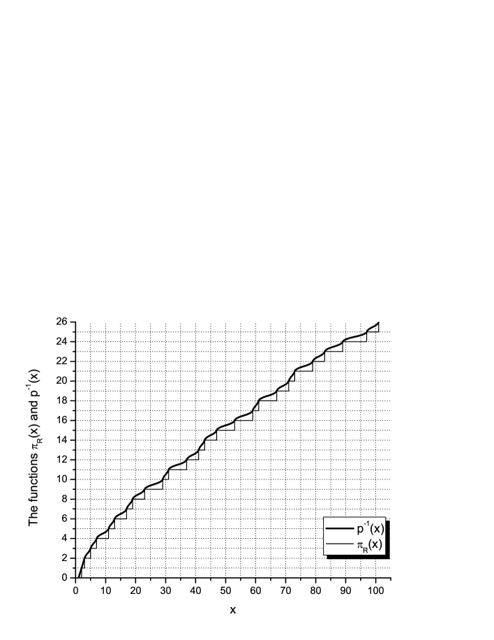
Figure 1: The Riemann–von Mangoldt counting step function $\pi_{R}(x)$ and its continuously differentiable analog $p^{-1}(x)$.

The comparative plot of the functions $p^{-1}(x)$ and $\pi_{R}(x)$ is shown on Fig. 1. The derivative $dp^{-1}/dx$ is shown on Fig. 2. Its oscillating nature as well as the fact that it takes values between $0$ and $1$ is obvious from this figure.

Figure 2: The derivative of $p^{-1}(x)$

The diffeomorphisms $p(x)$, $p^{-1}(x)$ and their derivatives are realized in a Fortran90 program package called pp_.f90 which can be found at this URL [3].

3 Approximate solution of Diophantine equations

Definition 2

Given a set of strictly increasing functions $h_{i}(x)\in C^{(1)}(0,\infty)$, $i=1,\ldots n$ the system

$$f_{1}(x_{1},\ldots,x_{n})=0,$$ (24)

$$f_{2}(h_{1}(x_{1}),\ldots,h_{n}(x_{n})):=\sum\limits_{i=1}^{n}\sin^{2}(\pi h_{i}(x_{i}))=0,$$ (25)

where Eq. (24) is a Diophantine one is called real-Diophantine on the real semi axis $(0,\infty)$.

The real-Diophantine systems allow us to find solutions of Diophantine equations in terms of real approximations of integer numbers. For this purpose one should apply numerical methods which work even when the derivative is degenerate at the solution (see, e.g., [4] and [5]).

Let us write the system (24), (25) in a vector form as follows

$$Fx=0,$$ (26)

where

$$Fx={f^{\prime}}^{T}(x)fx,\quad fx=\left[f_{1}(x),f_{2}(x)\right]^{T},\quad f:D_{f}\subset\mathbb{R}^{n}\to\mathbb{R}^{m},\quad x\in\mathbb{R}^{n},\quad n>m,$$

$f^{\prime}(x)$ is the Jacobi matrix and $D_{f}$ is an open convex domain in $\mathbb{R}^{n}$.

Here we shall quote an autoregularized version of the Gauss–Newton method [6, 7] as one of the possible methods for the solution of Eq. (26):

$$x^{0}\in D_{f},\quad\epsilon_{0}>0,\quad \left({f^{\prime}}^{T}(x^{k})f^{\prime}(x^{k})+\epsilon_{k}I\right)(x^{k+1}-x^{k})=-Fx^{k},\quad k=1,2,\ldots\;.$$

$$\epsilon_{k}=\frac{1}{2}\left(\sqrt{\tau_{k}^{2}+4c\rho_{k}}-\tau_{k}\right),$$

$$\tau_{k}=||{f^{\prime}}^{T}(x^{k})f^{\prime}(x^{k})||_{\infty},\quad\rho_{k}=||Fx^{k}||_{\infty},\quad c=\frac{\epsilon_{0}+\epsilon_{0}\tau_{0}}{\rho_{0}},$$

where $||\cdot||_{\infty}$ is the uniform vector or matrix norm, and the SVD method [8] is assumed for the solution of the linear problem in (3). In order to find all solutions of Eq. (26) in the domain $D_{f}$ the vector $Fx^{k}$ is repeatedly multiplied by the local root extractor

$$e_{j}(x,\bar{x}^{(j)})=\frac{1}{1-\exp\left(-||x-\bar{x}^{(j)}||_{2}^{2}\right)},$$

in which $\bar{x}^{(j)}$ is the $j$-th solution of Eq. (26). In the repeated solutions of the transformed problem

$$F_{J}\,x:=\left(\prod_{j=1}^{J}e_{j}(x,\bar{x}^{(j)})\right)Fx=0,\quad J\geq 1,$$ (28)

the process (3) is executed with a new $Fx:=F_{J}x$. For every solution the process (3) is started many times with different $x^{0}$ and $\epsilon_{0}$. Each time when $J$ increases the derivatives $f^{\prime}(x_{k})$ are computed analytically and the matrices ${f^{\prime}}^{T}(x_{k})f^{\prime}(x_{k})$ are adaptively scaled [9]. The necessary last step of the method consists in a direct substitution check whether the Diophantine equation residual vanishes exactly when the found solutions are rounded to integers.

The system (24), (25) has been considered in Refs. [10] and [11] (pp. 285–286) as undecidable. In Table 1 we present some examples in which the real-Diophantine system (24), (25) is solvable including the case when it is solvable over the primes (see cases 2, 3, 4 and 6).

Table 1: Real-Diophantine systems: when $h_{i}(x_{i})=x_{i}$ the solution is looked for among the integers while $h_{i}(x_{i})=p^{-1}(x_{i})$ means that the solution would be among the primes.

case	$f_{1}(x)$	$n$	$m$	$h_{i}(x_{i})$	source
1	$x_{1}^{2}+x_{2}^{2}-x_{3}^{2}=0$	3	2	$x_{i}$	Pythagoras
2	$x_{1}^{2}+x_{2}^{2}-x_{3}^{2}-1=0$	3	2	$p^{-1}(x_{i})$	Sierpinski
3	$x_{1}^{2}+x_{2}^{2}+x_{3}^{2}+x_{4}^{2}=n,\ n\in\mathbb{N}$	4	2	$p^{-1}(x_{i})$	Lagrange
4	$\sum\limits_{i=1}^{9}x_{i}^{3}=n,\ n\in\mathbb{N}$	9	2	$x_{i},\ p^{-1}(x_{i})$	Waring, Khinchin
5	$\sum\limits_{i=1}^{19}x_{i}^{4}=n,\ n\in\mathbb{N}$	19	2	$x_{i}$	Waring
6	$\left(x_{1}/x_{2}\right)^{2}-\left(x_{3}/x_{4}\right)^{3}-x_{5}=0$	5	2	$h_{i}(x_{i})=p^{-1}(x_{i})$,	Fermat–Bache
				$i=1,\ldots,4$, $h_{5}(x_{5})=x_{5}$

Here we shall describe in more detail two special examples which emphasize the crucial role of the last step of the above method. In the first one we represent the prime number $5081$ as a sum of $9$ cubes of primes (case $4$ in Table 1 with $h_{i}(x_{i})=p^{-1}(x_{i})$). We find two different solutions:

$$5081=\left\{\begin{array}[]{l}2\times 2^{3}+3\times 3^{3}+5^{3}+2\times 11^{3}+13^{3}\;,\\ 3^{3}+3\times 5^{3}+2\times 7^{3}+3\times 11^{3}\;.\end{array}\right.$$ (29)

Notice that this problem has been solved as a real-Diophantine system on a machine with $16$ significant figures. The unknowns $2,\ 3,\ 5,\ 7,\ 11$ and $13$ in the first line of Eq. (29) have been found with $9$ significant figures at residual $||f_{1}(x)||_{\infty}=10^{-14}$. A convergent process of the kind (3) has been build after $36$ unsuccessful attempts which costed $5634$ iterations with $4$ different initial guesses $x_{0}$ combined with $9$ different initial regularizators $\epsilon_{0}$. The last step of the method yields an exact equality in Eq. (29). It would be interesting to investigate whether the number of primes which can be represented as the sum of $9$ prime cubes is infinite.

In the second example we consider the equation

$$\left(\frac{x_{1}}{x_{2}}\right)^{2}-\left(\frac{x_{3}}{x_{4}}\right)^{3}=x_{5},$$ (30)

where $x_{i}$, $i=1,2,3,4$ are sought as primes while $x_{5}$ as integer (special case of the unsolved Fermat–Bache problem in which the solutions are a rational pair $(x_{1}/x_{2},\ x_{3}/x_{4})$ and an integer $x_{5}$). The approximate solution found under conditions similar to those in the previous example, Eq. (29),

$$x_{1}=787.000011,\quad\quad x_{2}=348.99999357,\quad x_{3}=457.00002128,$$

$$x_{4}=1049.0000001,\quad x_{5}=5.0024058062,$$

leads to a nonzero residual after rounding to integers

$$\left(\frac{787}{349}\right)^{2}-\left(\frac{457}{1049}\right)^{3}-5=0.002405488240.$$

This example is an illustration of the crucial importance of the last step of the method–the vector $(787,\ 349,\ 457,\ 1049,\ 5)$ is not a true solution of the Fermat–Bache equation (30).

The above method for the solution of Diophantine equations works because of a combination of factors: autoregularization, SVD method, adaptive scaling, and because the solutions of Diophantine equations are well isolated. There is a semi-local convergence theory [6] in the non-degenerate case however no justification in the degenerate case is available by now. The methods of Refs. [4, 5] are applied to this problem with little success.

Remark 2

The method (24), (25) for the solution of the Diophantine equation (24) does not contradict the negative solution of the 10-th Hilbert’s problem [12] because our solutions are approximated in a bounded domain.

4 The function $p^{-1}(x)$ and the Riemann hypothesis

Lemma 2

The functions $p^{-1}(x)$ and $\pi(x)$ are related by

$$|p^{-1}(x)-\pi(x)|\leq 1\quad\forall x>1.$$

Proof: Let us assume that $p_{n}\leq x\leq p_{n+1}$ for some $n$. According to Eq. (20) the function $p^{-1}(x)$ is strictly increasing, i.e., $p^{-1}(x)\leq p^{-1}(p_{n+1})$. On the other hand $\pi(p_{n})\leq\pi(x)\leq\pi(p_{n+1})$ so that

$$|p^{-1}(x)-\pi(x)|\leq|p^{-1}(p_{n+1})-\pi(p_{n})|=|n+1-n|=1,$$

where we have used that $p^{-1}(p_{n})=n$ which follows from Theorem 1 and Eq. (5).

$\Box$

Theorem 2

The asymptotics of $p^{-1}(x)$ is the same as that for $\pi(x)$ when $x\to\infty$.

Proof: Let us consider the relative difference of $\pi(x)$ and $\mathrm{Li}(x)$. According to Lemma 2 we can write

$$\frac{|\pi(x)-\mathrm{Li}(x)|}{\mathrm{Li}(x)}\leq\frac{|\pi(x)-p^{-1}(x)|}{\mathrm{Li}(x)}+\frac{|p^{-1}(x)-\mathrm{Li}(x)|}{\mathrm{Li}(x)}\leq\frac{1}{\mathrm{Li}(x)}+\frac{|p^{-1}(x)-\mathrm{Li}(x)|}{\mathrm{Li}(x)}.$$

Therefore in the limit $x\to\infty$ we can ignore the term $1/\mathrm{Li}(x)$ and investigate $p^{-1}(x)$ instead of $\pi(x)$.

$\Box$

4.1 Differential equation and the von Koch estimate

Let us consider the following function

$$K(x)=\frac{p^{-1}(x)-\mathrm{Li}(x)}{\sqrt{x}\,\ln(x)},\quad x>1,$$ (31)

where $\mathrm{Li}(x)$ is defined in Eq. (1). According to the von Koch estimate (see [1], pp. 90) the Riemann hypothesis is equivalent to the statement that $K(x)$ is asymptotically constant, i.e.,

$$\lim_{x\to\infty}K(x)=\mathrm{const.}\quad\Longleftrightarrow\quad\mathrm{RH}.$$

Because the function $p^{-1}(x)$ is continuously differentiable we can write the following differential equation for $K$

$$K^{\prime}(x)=-\left(\frac{1}{2x}+\frac{1}{x\,\ln(x)}\right)K(x)+\frac{\frac{dp^{-1}(x)}{dx}-\frac{1}{\ln(x)}}{\sqrt{x}\,\ln(x)}.$$ (32)

The derivative $dp^{-1}(x)/dx$ is strongly oscillating as shown on Fig. 2, however it is restricted between $0$ and $1$ according to Eq. (20). Therefore we shall consider the solution of Eq. (32) in the interval $p_{n}\leq x\leq(p_{n}+p_{n+1})/2$, $n\to\infty$, and shall use the fact that (see Eqs. (14) and (16))

$$\left.\frac{dp^{-1}(x)}{dx}\right|_{x=p_{n}}=1,\quad\left.\frac{dp^{-1}(x)}{dx}\right|_{x=(p_{n}+p_{n+1})/2}=\frac{1}{2\hat{p}_{n}+1}.$$ (33)

Thus, for $x\to p_{n}$ we can substitute $dp^{-1}/dx=1$ in Eq. (32), neglect the term $1/\ln(x)$ in the limit $x\to\infty$ and solve the equation

$$K^{\prime}(x)=-\left(\frac{1}{2x}+\frac{1}{x\,\ln(x)}\right)K(x)+\frac{1}{\sqrt{x}\,\ln(x)}.$$ (34)

The general solution of this equation can be written as

$$K(x)=\frac{\sqrt{x}}{\ln(x)}+\frac{{c^{\prime}}_{n}}{\sqrt{x}\,\ln(x)},$$

where the first term in the right-hand-side is a partial solution of the inhomogeneous equation (34) while the second one is the general solution of the homogeneous equation and $c^{\prime}_{n}$ is a constant.

At the right-hand border $x\to(p_{n}+p_{n+1})/2$, we can neglect, for $x\to\infty$, the term $dp^{-1}/dx=(2\hat{p}_{n}+1)^{-1}$ and keep only $1/\ln(x)$ assuming that $\hat{p}_{n}\sim p_{n}^{\alpha}$ with $\alpha>0$. In this case we should solve the equation

$$K^{\prime}(x)=-\left(\frac{1}{2x}+\frac{1}{x\,\ln(x)}\right)K(x)+\frac{-1}{\sqrt{x}\,\ln^{2}(x)}.$$ (35)

The general solution of (35) is again the sum of a partial solution (the first term bellow) of the inhomogeneous equation and the general solution (the second term) of the homogeneous one

$$K(x)=-\frac{\mathrm{Li}(x)}{\sqrt{x}\,\ln(x)}+\frac{{c^{\prime\prime}}_{n}}{\sqrt{x}\,\ln(x)}.$$

Substituting the logarithmic integral with its leading term for $x\to\infty$, i.e., $\mathrm{Li}(x)\sim x/\ln(x)$ we can finally write

$$K(x)\sim\left\{\begin{array}[]{rl}\frac{\sqrt{x}}{\ln(x)}+\frac{c^{\prime}_{n}}{\sqrt{x}\,\ln(x)},&x\to p_{n}\\ -\frac{\sqrt{x}}{\ln^{2}(x)}+\frac{{c^{\prime\prime}}_{n}}{\sqrt{x}\,\ln(x)},&x\to\frac{p_{n}+p_{n+1}}{2}\end{array}\right.$$

It is tempting to regard the general solution of the homogeneous equation as subleading in the limit $x\to\infty$ and the first terms as expressing the oscillations of $K(x)$ close to the borders of the considered intervals. However, let us note that the constants $c^{\prime}_{n}$ and ${c^{\prime\prime}}_{n}$ might depend on the primes gap $\hat{p}_{n}$ which on its own depends on $p_{n}$ and this last dependence is currently unknown.

4.2 The l’Hospital rule

Here we shall consider the limit

$$\lim_{x\to\infty}\frac{p^{-1}(x)-\mathrm{Li}(x)}{\mathrm{Li}(x)}=\lim_{x\to\infty}\frac{p^{-1}(x)}{\mathrm{Li}(x)}-1$$

Because the function $p^{-1}(x)$ is differentiable we can apply the l’Hospital rule if the limit

$$\lim_{x\to\infty}\frac{\frac{dp^{-1}(x)}{dx}}{\frac{1}{\ln(x)}}=\lim_{x\to\infty}\ln(x)\frac{dp^{-1}(x)}{dx}$$

exists. Now let us show that if the RH is true then this limit does not exist. Indeed, let us choose two subsequences of $x\to\infty$, namely

$$(i) \quad x=p_{n},\qquad\qquad n\to\infty,$$

$$(ii) \quad x=\frac{p_{n}+p_{n+1}}{2},\quad n\to\infty.$$ (36)

Then, using again the values (33) of the derivative over (i) and (ii) we get

$$(i) \quad\ln(x)\frac{dp^{-1}(x)}{dx}\sim\ln(p_{n})\to\infty,$$

$$(ii) \quad\ln(x)\frac{dp^{-1}(x)}{dx}\sim\frac{\ln(p_{n})}{2\hat{p}_{n}+1}\to 0.$$ (37)

The second limit follows from the statement that if the RH is true then $\hat{p}_{n}\sim p_{n}^{\frac{1}{2}+\epsilon}$ for any $\epsilon>0$ when $n\to\infty$ [2]. Most of the current estimates of the primes gap $\hat{p}_{n}$ lead to the non-applicability of the l’Hospital rule. Nevertheless we cannot be sure until a rigorous estimate is found.

5 Conclusions

We have constructed a pair of diffeomorphisms $p(x)$ and $p^{-1}(x)$ which interpolate the prime series and the prime counting function, respectively, which are convenient for both numerical and analytical applications. To the best of our knowledge this is the first differentiable and invertible interpolation of the prime series.

The function $p^{-1}(x)$ can be effectively used for the solution of Diophantine equations which can be exploited in many cases where the other methods do not work and could be particularly useful when Diophantine equations are subsystems of more complex real systems.

Because $p^{-1}(x)$ has the same behavior as $\pi(x)$ for $x\to\infty$ it could give more information about the asymptotic and non-asymptotic distribution of primes. Perhaps, this could be used to draw some conclusions about the Riemann hypothesis when more information about the primes gaps becomes available.

Acknowledgments

The authors thank the BLTPh laboratory JINR, Dubna for hospitality and support. LG has been partially supported by the FP5-EUCLID Network Program of the European Commission under Contract No. HPRN-CT-2002-00325 and by the Bulgarian National Foundation for Scientific Research under Contract No. Ph-1406.

References

- [1] H.M. Edwards, Riemann’s Zeta Function, Dover Publication, Mineola, New York (2001).
- [2] R. Crandall, Carl Pomerance, Prime Numbers: A Computational Perspective, Springer, New York (2002).
-
[3]
L. Georgiev’s homepage:
http://theo.inrne.bas.bg/lgeorg/pp
_.html - [4] L. Alexandrov, Regularized trajectories for Newton kind approximations of the solutions of nonlinear equations, Differential Equations, XIII, No. 7, 1281–1292 (1977, Russian).
- [5] B. Kaltenbacher, A. Neubauer, and A.G. Ramm, Convergence of the continuous regularized Gauss–Newton method, J. Inv. Ill-Posed Problems, 10, No. 3, 261–280 (2002).
- [6] L. Alexandrov, Regularized Newton–Kantorovich computational processes, J. Compt. Math. Math. Phys., 11, 36–43 (1971, Russian)
- [7] L. Alexandrov, Autoregularized Newton–Kantorovich iterational processes, JINR Commun. P5-5515, Dubna, 1970.
- [8] G.H. Golub, C. Reinish, Singular Value Decomposition and Least Squares, in Handbook for automatic computation, J.H. Wilkinson and C. Reinish, Eds., v. II, Linear Algebra, Heidelberg, Springer, 1971.
- [9] J.J. More, The Levenberg–Marquardt algorithm, in Numerical Analysis, G.A. Watson, Ed., Lecture Notes in Math., 630, Springer, Berlin 105–116 (1977).
- [10] N.C.A. da Costa, and F.A. Doria, Undecidability and incompleteness in Classical Mechanics, Int. J. Theor. Phys., 30, No. 8, 1041–1073 (1991).
- [11] S. Smale, Mathematical Problems for the Next Century, in Mathematics: Frontiers and Perspectives, V. Arnold et.al., Eds., 271–294, AMS, Providence, USA (2000).
- [12] Y. Matiyasevich, Hilbert’s Tenth Problem, The MIT Press, Cambridge, Mass. (1993).