Alternative perturbation approaches in classical mechanics

Abstract

We discuss two alternative methods, based on the Lindstedt–Poincaré technique, for the removal of secular terms from the equations of perturbation theory. We calculate the period of an anharmonic oscillator by means of both approaches and show that one of them is more accurate for all values of the coupling constant.

I Introduction

Straightforward application of perturbation theory to periodic nonlinear motion gives rise to secular terms that increase in time in spite of the fact that the trajectory of the motion is known to be bounded N81 ; F00 . One of the approaches commonly used to remove those unwanted secular terms is the method of Lindstedt–Poincaré N81 ; F00 , recently improved by Amore et al. AA03 ; AL04 by means of the delta expansion and the principle of minimal sensitivity.

There is also another technique that resembles the method of Lindstedt–Poincaré which is suitable for the removal of secular terms M70 . Discussion and comparison of such alternative approaches may be most fruitful for teaching perturbation theory in advanced undergraduate courses on classical mechanics.

In Sec. II we present a simple nonlinear model to which we apply the alternative perturbation approaches in subsequent sections. In Sec. III we apply straightforward perturbation theory and illustrate the outcome of secular terms. In Sec. IV we show how to remove those secular terms by means of the Lindstedt–Poincaré method N81 ; F00 . In Sec. V we develop an alternative method that appears in another textbook M70 and that closely resembles the method of Lindstedt–Poincaré. In Sec. VI we describe an improvement to the method of Lindstedt–Poincaré proposed by Amore et al. AA03 ; AL04 . Finally, in Sec. VII we compare the period of the motion calculated by all those approaches.

II The Model

In order to discuss and compare the alternative perturbation approaches mentioned above, we consider the simple, nonlinear equation of motion

$$\ddot{x}(t)+x(t)=-\lambda x^{3}(t)$$ (1)

with the initial conditions $x(0)=1$ and $\dot{x}(0)=0$. In Appendix A we show that we can derive this differential equation from the equation of motion for a particle of mass $m$ in a polynomial anharmonic potential with arbitrary quadratic and quartic terms. Notice that $E=\dot{x}^{2}/2+x^{2}/2+\lambda x^{4}/4=1/2+\lambda/4$ is an integral of the motion for (1) and that the motion is periodic for all $\lambda>-1$ for the initial conditions indicated above.

III Secular Perturbation Theory

The straightforward expansion of $x(t)$ in powers of $\lambda$

$$x(t)=\sum_{j=0}^{\infty}x_{j}(t)\lambda^{j}$$ (2)

leads to the perturbation equations

$$\ddot{x}_{0}(t)+x_{0}(t) = 0$$

$$\ddot{x}_{1}(t)+x_{1}(t) = -x_{0}^{3}(t)$$

$$\ddot{x}_{n}(t)+x_{n}(t) = -\sum_{j=0}^{n-1}\sum_{k=0}^{j}x_{k}(t)x_{j-k}(t)x_{n-j-1}(t),\;n=2,3,\ldots$$ (3)

with the boundary conditions $x_{j}(0)=\delta_{j0}$ and $\dot{x}_{j}(0)=0$ for all $j\geq 0$. Clearly, the solution of order zero is $x_{0}(t)=\cos(t)$.

All those perturbation equations are of the form $\ddot{y}(t)+y(t)=f(t)$, where $f(t)$ is a linear combination of $\cos(jt)$, $j=1,2,\ldots$. Such differential equations, which are commonly discussed in introductory calculus courses, are in fact suitable for illustrating the advantage of using available computer algebra systems.

It is well known that any term proportional to $\cos(t)$ in $f(t)$ gives rise to a secular term after integration N81 ; F00 . For example, since $x_{0}^{3}(t)=[\cos(3t)+3\cos(t)]/4$ we obtain

$$x_{1}(t)=\frac{1}{8}\left[\frac{\cos(3t)-\cos(t)}{4}-3t\sin(t)\right]$$ (4)

that clearly shows that $|x_{1}(t)|$ grows unboundedly with time in spite of the fact that the exact motion is periodic for all $\lambda>-1$.

IV Method of Lindstedt–Poincaré

There are several suitable mathematical techniques that overcome the problem of secular terms mentioned above N81 . For example, the method of Lindstedt–Poincaré is based on the change of the time variable

$$s=\sqrt{\gamma}t$$ (5)

where $\sqrt{\gamma}$ plays the role of the frequency of the motion, and, therefore, the period $T$ is given by

$$T=\frac{2\pi}{\sqrt{\gamma}}.$$ (6)

The equation of motion (1) thus becomes

$$\gamma x^{\prime\prime}(s)+x(s)=-\lambda x^{3}(s)$$ (7)

where the prime stands for differentiation with respect to $s$. If we expand both $x(s)$ and $\gamma$ in powers of $\lambda$

$$\gamma=\sum_{j=0}^{\infty}\gamma_{j}\lambda^{j}$$ (8)

with $\gamma_{0}=1$, then we obtain the set of equations

$$x_{0}^{\prime\prime}(s)+x_{0}(s) = 0$$

$$x_{1}^{\prime\prime}(s)+x_{1}(s) = -x_{0}^{3}(s)-\gamma_{1}x_{0}^{\prime\prime}(s)$$

$$x_{n}^{\prime\prime}(s)+x_{n}(s) = -\sum_{j=0}^{n-1}\sum_{k=0}^{j}x_{k}(s)x_{j-k}(s)x_{n-j-1}(s)-\sum_{j=1}^{n}\gamma_{j}x_{n-j}^{\prime\prime}(s),\;$$

$$n = 2,3,\ldots$$ (9)

We choose the value of the coefficient $\gamma_{n}$ in order to remove the secular term from the perturbation equation of order $n$. For example, it follows from $-x_{0}^{3}-\gamma_{1}x_{0}^{\prime\prime}=\left(\gamma_{1}-3/4\right)\cos(t)-\cos(3t/4)$ that $\gamma_{1}=3/4$ is the right choice at first order. Proceeding exactly in the same way at higher orders we obtain the coefficients

$$\gamma_{1}=\frac{3}{4}\ \ ,\ \ \gamma_{2}=-\frac{3}{128}\ \ ,\ \ \gamma_{3}=\frac{9}{512}$$ (10)

and the approximate period

$$T=\frac{32\sqrt{2}\pi}{\sqrt{\left(9\lambda^{3}-12\lambda^{2}+384\lambda+512\right)}}$$ (11)

V Alternative Lindstedt–Poincaré Technique

Perturbation theory provides a $\lambda$–power series for the frequency of the motion $\omega$; for example, for our model it reads

$$\omega^{2}=1+w_{1}\lambda+w_{2}\lambda^{2}+\ldots$$ (12)

An alternative perturbation approach free from secular terms is based on the substitution of this expansion into the equation of motion (1) followed by an expansion of the resulting equation

$$\ddot{x}(t)+\left(\omega^{2}-w_{1}\lambda-w_{2}\lambda^{2}+\ldots\right)x(t)=-\lambda x^{3}(t)$$ (13)

in powers of $\lambda$, as if $\omega$ were independent of the perturbation parameter M70 . The perturbation equations thus produced read

$$\ddot{x}_{0}(t)+\omega^{2}x_{0}(t) = 0$$

$$\ddot{x}_{1}(t)+\omega^{2}x_{1}(t) = -x_{0}^{3}(t)+w_{1}x_{0}(t)$$

$$\ddot{x}_{n}(t)+\omega^{2}x_{n}(t) = -\sum_{j=0}^{n-1}\sum_{k=0}^{j}x_{k}(t)x_{j-k}(t)x_{n-j-1}(t)-\sum_{j=1}^{n}w_{j}x_{n-j}(t),\;$$

$$n = 2,3,\ldots.$$ (14)

Notice that $x_{0}=\cos(\omega t)$ depends on $\omega$ and so does each coefficient $w_{n}$ that we set to remove the secular term at order $n$. Consequently, we have to solve the partial sums arising from truncation of the series (12) for $\omega$ in order to obtain the frequency and the period

$$T=\frac{2\pi}{\omega}.$$ (15)

in terms of $\lambda$ M70 .

A straightforward calculation through third order yields

$$w_{1} = \frac{3}{4}\ \ ,\ \ w_{2}=-\frac{3}{128\omega^{2}}\ \ ,\ \ w_{3}=0$$ (16)

from which we obtain

$$\omega=\frac{\sqrt{\left(\sqrt{30\lambda^{2}+96\lambda+64}+2(3\lambda+4)\right)}}{4}$$ (17)

VI Variational Lindstedt–Poincaré

Amore et al. AA03 ; AL04 have recently proposed a variational method for improving the Lindstedt–Poincaré technique. It consists of rewriting equation (1) as

$$\ddot{x}(t)+\left(1+\alpha^{2}\right)x(t)=\delta\left(-\lambda x^{3}(t)+\alpha^{2}x(t)\right)$$ (18)

where $\alpha$ is an adjustable variational parameter, and $\delta$ is a dummy perturbation parameter that we set equal to unity at the end of the calculation. When $\delta=1$ the modified equation of motion (18) reduces to equation (1) that is independent of $\alpha$. Following the Lindstedt–Poincaré technique we change the time variable according to equation (5) thus obtaining

$$\gamma x^{\prime\prime}(s)+(1+\alpha^{2})x(s)=\delta\left(-\lambda x^{3}(s)+\alpha^{2}x(s)\right).$$ (19)

We then expand both $x$ and $\gamma$ in powers of $\delta$ and proceed exactly as is Sec. IV, except that in this case $\gamma_{0}=1+\alpha^{2}$. Thus we obtain

$$x_{0}^{\prime\prime}(s)+x_{0}(s) = 0$$

$$x_{1}^{\prime\prime}(s)+x_{1}(s) = \frac{1}{\gamma_{0}}\left(-\lambda x_{0}^{3}(s)-\gamma_{1}x_{0}^{\prime\prime}(s)+\alpha^{2}x_{0}(s)\right)$$

$$x_{n}^{\prime\prime}(s)+x_{n}(s) = \frac{1}{\gamma_{0}}\left(-\sum_{j=0}^{n-1}\sum_{k=0}^{j}x_{k}(s)x_{j-k}(s)x_{n-j-1}(s)\right.\;$$ (20)

$$\left.-\sum_{j=1}^{n}\gamma_{j}x_{n-j}^{\prime\prime}(s)+\alpha^{2}x_{n-1}(s)\right),\;n=2,3,\ldots.$$

The period of the motion is given by equation (6).

Choosing the value of $\gamma_{n}$ in order to remove the secular term from the perturbation equation of order $n$ we obtain

$$\gamma_{1}=\frac{3\lambda-4\alpha^{2}}{4}\ \ ,\ \ \gamma_{2}=-\frac{3\lambda^{2}}{128\left(1+\alpha^{2}\right)}\ \ ,\ \ \gamma_{3}=\frac{3\lambda^{2}\left(3\lambda-4\alpha^{2}\right)}{512\left(1+\alpha^{2}\right)^{2}}.$$ (21)

Notice that these coefficients reduce to those in equation (10) (multiplied by the proper power of $\lambda$) when $\alpha=0$. Since the actual value of $\gamma$ is independent of $\alpha$ when $\delta=1$, we make use of the principle of minimal sensitivity developed in Appendix B. The root of

$$\frac{d}{d\alpha}\sum_{j=0}^{3}\gamma_{j}=0$$ (22)

is

$$\alpha=\frac{\sqrt{3\lambda}}{2}$$ (23)

and we thus obtain

$$T=\frac{8\sqrt{2}\pi(3\lambda+4)}{\sqrt{\left(207\lambda^{3}+852\lambda^{2}+1152\lambda+512\right)}}.$$ (24)

For this particular problem we find that the value of $\alpha$ given by the PMS condition (23) is such that $\gamma_{2j+1}=0$ for all $j\geq 0$.

VII Results and Discussion

Fig. 1 shows the period as a function of $\lambda$ given by the perturbation approaches discussed above and by the exact expression N81

$$T=\frac{2}{\sqrt{1+\lambda}}\int_{0}^{\pi}\frac{d\theta}{\sqrt{1-\frac{\lambda\sin(\theta)^{2}}{2(1+\lambda)}}}.$$ (25)

We appreciate that the variational Lindstedt–Poincaré method AA03 ; AL04 yields more accurate results than the straightforward Lindstedt–Poincaré technique N81 ; F00 , and that the alternative Lindstedt–Poincaré approach M70 is the best approach, at least at third order of perturbation theory.

All those expressions yield the correct value $T(0)=2\pi$ and become less accurate as $\lambda$ increases. However, two of them give reasonable results even in the limit $\lambda\rightarrow\infty$. The exact value is

$$\lim_{\lambda\rightarrow\infty}\sqrt{\lambda}T^{exact}=2\sqrt{2}\int_{0}^{\pi}\frac{d\theta}{\sqrt{1+\cos(\theta)^{2}}}=7.4162987.$$ (26)

The standard Lindstedt–Poincaré technique fails completely as shown by

$$\lim_{\lambda\rightarrow\infty}\sqrt{\lambda}T^{LP}=0.$$ (27)

The variational improvement proposed by Amore et al. AA03 ; AL04 corrects this anomalous behavior

$$\lim_{\lambda\rightarrow\infty}\sqrt{\lambda}T^{VLP}=\frac{8\sqrt{46}\pi}{23}=7.4112410.$$ (28)

Finally, the alternative Lindstedt–Poincaré method M70 gives the closest approach

$$\lim_{\lambda\rightarrow\infty}\sqrt{\lambda}T^{ALP}=\pi\sqrt{\left(64-\frac{32\sqrt{30}}{3}\right)}=7.4185905.$$ (29)

Appendix A Dimensionless equations

Transforming an equation of physics into a dimensionless mathematical equation is most convenient for at least two reasons. First, the latter is much simpler and reveals more clearly how it can be solved. Second, the dimensionless equation exhibits the actual dependence of the solution on the parameters of the physical model.

In order to illustrate how to convert a given equation into a dimensionless one we consider a particle of mass $m$ moving in the potential

$$V(q)=\frac{v_{2}}{2}q^{2}+\frac{v_{4}}{4}q^{4}.$$ (30)

The equation of motion is

$$m\ddot{q}=-v_{2}q-v_{4}q^{3}$$ (31)

and we assume that $q(0)=q_{0}$ and $\dot{q}(0)=v_{0}$.

We define a new independent variable $s=\omega_{0}t+\phi$, where $\phi$ is a phase, and $\omega_{0}=\sqrt{v_{2}/m}$ is the frequency of the motion when $v_{4}=0$. Suppose that $\dot{q}=0$ and $q=A$ at $t=t_{1}$; then we define the dependent variable $x(s)=q(t)/A$ and choose $\phi=-\omega_{0}t_{1}$ so that $x(s)$ is a solution of the differential equation

$$x^{\prime\prime}(s)+x(s)=-\lambda x(s)^{3}$$ (32)

where $\lambda=v_{4}A^{2}/v_{2}$ and the initial conditions become $x(0)=1$ and $x^{\prime}(0)=0$.

The dimensionless differential equation (32) resembles the equation of motion for a particle of unit mass moving in the potential $V(x)=x^{2}/2+\lambda x^{4}/4$. Its period $T$ depends on $\lambda$ and, therefore, the expression for the period of the original problem $T^{\prime}=T/\omega_{0}$ clearly reveals the way it depends upon the model parameters $m$, $v_{2}$, $v_{4}$, and $A$.

Appendix B Variational perturbation theory

Variational perturbation theory is a well–known technique for obtaining an approximation to a property $P(\lambda)$ in a wide range of values of the parameter $\lambda$. Suppose that $P(\lambda)$ is a solution of a given equation of physics $F(\lambda,P)=0$ that we are unable to solve exactly. In some cases we can obtain an approximation to $P(\lambda)$ in the form of a power series $P(\lambda)=P_{0}+P_{1}\lambda+\ldots$ by means of perturbation theory. If this series is divergent or slowly convergent we may try and improve the results by means of a resummation technique.

Variational perturbation theory consists of modifying the physical equation in the form $F(\xi,\alpha,\lambda,P)=0$, where $\alpha$ is a variational parameter (or a set of them in a more general case) and $\xi$ is a dummy perturbation parameter so that $F(1,\alpha,\lambda,P)=F(\lambda,P)$.

Then we apply perturbation theory in the usual way, calculate $N+1$ coefficients of the perturbation series

$$P(\xi,\alpha,\lambda)=\sum_{j=0}^{\infty}P_{j}(\alpha,\lambda)\xi^{j}$$ (33)

and construct an approximation of order $N$ to the property

$$P^{[N]}(\alpha,\lambda)=\sum_{j=0}^{N}P_{j}(\alpha,\lambda).$$ (34)

If the partial sums $P^{[N]}(\alpha,\lambda)$ converged toward the actual property as $N\rightarrow\infty$, then $P^{[\infty]}(\alpha,\lambda)=P(\lambda)$ would be independent of $\alpha$. However, for finite $N$ the partial sums do depend on the variational parameter $\alpha$. It is therefore reasonable to assume that the optimum value of this parameter should be given by the principle of minimal sensitivity (PMS) S81 :

$$\left.\frac{\partial}{\partial\alpha}P^{[N]}(\alpha,\lambda)\right|_{\alpha=\alpha_{N}(\lambda)}=0.$$ (35)

In many cases $P^{[N]}(\alpha_{N}(\lambda),\lambda)$ converges towards $P(\lambda)$ as $N\rightarrow\infty$, and, besides, $P^{[N]}(\alpha_{N}(\lambda),\lambda)$ behaves like $P(\lambda)$ with respect to $\lambda$ even at relatively small perturbation orders.

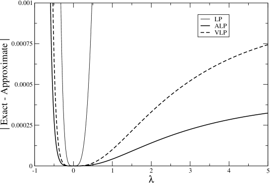
Figure 1: Absolute error on the period $\left|T_{exact}-T_{approx}\right|$ as a function of the coupling $\lambda$ for the Lindstedt-Poincaré (LP, solid thin line), the Alternative Lindstedt-Poincaré (ALP, solid bold line) and the Variational Lindstedt-Poincaré (VLP, dashed line) methods.

P.A. acknowledges support of Conacyt grant no. C01-40633/A-1.

References

• (1) A. H. Nayfeh, Introduction to Perturbation Techniques (John Wiley & Sons, New York, 1981).
• (2) F. M. Fernández, Introduction to Perturbation Theory in Quantum Mechanics (CRC Press, Boca Raton, 2000).
• (3) P. Amore and A. Aranda, Phys. Lett. A 316, 218 (2003).
• (4) P. Amore and H. Montes Lamas, Phys. Lett. A 327, 158 (2004).
• (5) J. Marion, Classical Dynamics of Particles and Systems, Second ed. (Academic, New York, 1970).
• (6) P. M. Stevenson, Phys. Rev. D 23, 2916 (1981).