SCD Patterns Have Singular Diffraction

Abstract.

Among the many families of nonperiodic tilings known so far, SCD tilings are still a bit mysterious. Here, we determine the diffraction spectra of point sets derived from SCD tilings and show that they have no absolutely continuous part, that they have a uniformly discrete pure point part on the axis $\mathbb{R}{\boldsymbol{e}}_{3}$, and that they are otherwise supported on a set of concentric cylinder surfaces around this axis. For SCD tilings with additional properties, more detailed results are given.

1. The tilings

After the discovery of families of tiles that permit only aperiodic tilings, the question arose whether there exists a single tile that permits only aperiodic tilings by copies of itself (an aperiodic prototile). A first example, which gives tilings in Euclidean 3–space, was found by P. Schmitt in 1988. It was elaborated later by J.H. Conway and L. Danzer (cf. [7]). In particular, they modified Schmitt’s prototile to a convex one. We refer to these tilings — which will be described in this section — as SCD tilings.

A tiling in $\mathbb{R}^{d}$ is a collection of tiles $\{T_{n}\}_{n\geq 0}$ which covers $\mathbb{R}^{d}$ and contains no overlapping tiles, i.e., $\operatorname{int}(T_{k})\cap\operatorname{int}(T_{n})=\varnothing$ for $k\neq n$. A tile is a nonempty compact set $T\subset\mathbb{R}^{d}$ with the property that $\operatorname{cl}(\operatorname{int}(T))=T$. A tiling ${\mathcal{T}}$ is called aperiodic, if ${\mathcal{T}}+{\boldsymbol{x}}={\mathcal{T}}$ implies ${\boldsymbol{x}}={\boldsymbol{0}}$.

The SCD tilings are built from a single kind of tile — a single prototile — which we refer to as SCD tile. Essentially, the main idea is that the only possible tilings are of the following form: The tiles can be put together to form layers, which extend in two dimensions; these layers can be stacked, but only in such a way that two consecutive layers are rotated against each other by an angle which may be incommensurate to $\pi$. Then, the symmetry groups of the resulting tilings may still be nontrivial, even infinite, but they contain no translation. To achieve this, we allow only directly congruent copies of the tiles, but no mirror images (cf. Section 3).

The SCD tile

Choose $0<\lambda<1$, and positive real numbers $b_{1},b_{2},c$. Let $\varphi=\arctan(b_{1}/b_{2})$, $a=\sqrt{b_{1}^{2}+b_{2}^{2}},$ and

$${\boldsymbol{a}}=(a,0,0),\,{\boldsymbol{b}}=(b_{1},b_{2},0),\,{\boldsymbol{c}}=\lambda{\boldsymbol{b}}+(0,0,c),\,{\boldsymbol{d}}=\lambda{\boldsymbol{a}}-(0,0,c),$$

(cf. Fig. 1). Now, we define the SCD tile as

(1) $$T=\operatorname{conv}({\boldsymbol{0}},{\boldsymbol{a}},{\boldsymbol{b}},{\boldsymbol{a}}+{\boldsymbol{b}},{\boldsymbol{c}},{\boldsymbol{a}}+{\boldsymbol{c}},{\boldsymbol{d}},{\boldsymbol{b}}+{\boldsymbol{d}}),$$

where $\operatorname{conv}(M)$ denotes the convex hull of $M$. The result is the union of the two triangular prisms $\operatorname{conv}({\boldsymbol{0}},{\boldsymbol{a}},{\boldsymbol{b}},{\boldsymbol{a}}+\boldsymbol{b},{\boldsymbol{c}},{\boldsymbol{a}}+{\boldsymbol{c}})$ and $\operatorname{conv}({\boldsymbol{0}},{\boldsymbol{a}},{\boldsymbol{b}},{\boldsymbol{a}}+{\boldsymbol{b}},{\boldsymbol{d}},{\boldsymbol{b}}+{\boldsymbol{d}})$, glued together at the rhomb–shaped facet $\operatorname{conv}({\boldsymbol{0}},{\boldsymbol{a}},{\boldsymbol{b}},{\boldsymbol{a}}+{\boldsymbol{b}})$. This is the reason that it is sometimes called Conway’s biprism. If $\varphi\notin\pi\mathbb{Q}$, we will call the SCD tile incommensurate (which is the classical case), otherwise commensurate.

We should mention that this is only one possible construction. Several generalizations or variations are possible (cf. Section 3 or [7]). But all these tiles give rise to tilings with basically the same structure.

The SCD tilings

Using translations of the SCD tile, one can put them together (i) by joining triangular facets $\operatorname{conv}({\boldsymbol{0}},{\boldsymbol{b}},{\boldsymbol{c}})$ with $\operatorname{conv}({\boldsymbol{a}},{\boldsymbol{a}}+{\boldsymbol{b}},{\boldsymbol{a}}+{\boldsymbol{c}})$, and (ii) by joining triangular facets $\operatorname{conv}({\boldsymbol{0}},{\boldsymbol{a}},{\boldsymbol{d}})$ with $\operatorname{conv}({\boldsymbol{b}},{\boldsymbol{b}}+{\boldsymbol{a}},{\boldsymbol{b}}+{\boldsymbol{d}})$. If we do so inductively until no triangular facet remains uncovered, we end up with a planar layer covering a 2–dimensional plane.

This layer is congruent to $L=\{{\boldsymbol{x}}+T\,|\,{\boldsymbol{x}}\in\varGamma\}$, where $\varGamma$ is the 2–dimensional point lattice spanned by ${\boldsymbol{a}}$ and ${\boldsymbol{b}}$, i.e., $\varGamma=\mathbb{Z}{\boldsymbol{a}}+\mathbb{Z}{\boldsymbol{b}}$. The top of $L$ shows ridges and valleys, all parallel to each other, and all parallel to ${\boldsymbol{b}}$. The bottom of $L$ also shows ’down under’ (or upside down) valleys and ridges, all of them parallel to ${\boldsymbol{a}}$. In order to stack the layers, consider a layer $L^{\prime}=L-{\boldsymbol{c}}$. Take a second layer $L^{\prime\prime}=(0,0,c)+RL^{\prime}$, where $R$ is a rotation through $-\varphi$ around the axis $\mathbb{R}{\boldsymbol{e}}_{3}=\langle(0,0,1)\rangle_{\mathbb{R}}$. $L^{\prime\prime}$ fits exactly on top of $L^{\prime}$. In the same fashion, we proceed stacking layers and obtain

(2) $${\mathcal{T}}=\bigcup_{m\in\mathbb{Z}}m(0,0,c)+R^{m}L^{\prime},$$

which is a tiling of $\mathbb{R}^{3}$. There are many other possibilities to build SCD tilings. E.g., two consecutive layers can be shifted against each other by an arbitrary translation in the direction of $R^{m}{\boldsymbol{b}}$, which is the direction of the matching valleys and ridges of the two layers. Let us mention that Danzer’s version restricts these translations to a discrete set $\mathbb{Z}R^{m}{\boldsymbol{b}}$ in order to allow crystallographic applications. Therefore, ’SC tilings’ might be a better notation for the more general tilings we consider here. Nevertheless, we will stick to the well–known notation of SCD tilings throughout this paper, holding in mind that the SCD tilings in [7] are a proper subset of the SCD tilings here. In this sense, all possible SCD tilings are congruent to

(3) $${\mathcal{T}}=\bigcup_{m\in\mathbb{Z}}m(0,0,c)+{\boldsymbol{v}}_{m}+R^{m}L^{\prime},$$

for some ${\boldsymbol{v}}_{m}=(v^{(m)}_{1},v^{(m)}_{2},0)$, where ${\boldsymbol{v}}_{m+1}-{\boldsymbol{v}}_{m}$ is a multiple of $R^{m}{\boldsymbol{b}}$. For a more thorough discussion of all possible SCD tilings, see Section 3 or [7].

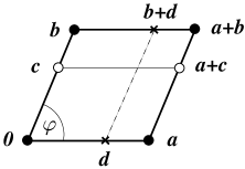
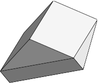
Figure 1. The construction of an SCD tile (left) and a view of an SCD tile (right)

As with tiles, we will distinguish between incommensurate SCD tilings, if they are built from incommensurate SCD tiles, and commensurate SCD tilings otherwise. Now, it is easy to see that incommensurate SCD tilings are aperiodic: Since $\varphi\notin\pi\mathbb{Q}$, all layers $m(0,0,c)+{\boldsymbol{v}}_{m}+R^{m}L$ have pairwise different orientations. Consequently, a possible translation ${\boldsymbol{x}}$ with ${\mathcal{T}}+{\boldsymbol{x}}={\mathcal{T}}$ must map every layer onto itself. The translation vectors that fix the $m$–th layer $m(0,0,c)+{\boldsymbol{v}}_{m}+R^{m}L$ are those in $R^{m}\varGamma$. So, the translation vectors which fix the whole tiling are elements of

$$\bigcap_{m\in\mathbb{Z}}R^{m}\varGamma=\{0\},$$

wherefore all incommensurate SCD tilings are aperiodic.

Note that even in the incommensurate case finitely many layers could still possess nontrivial translation symmetries, as two layers might still share a so-called coincidence site lattice $\varGamma^{\prime}$ of finite index in $\varGamma$. Then, any finite number of layers still may admit one, where the index grows with the number of layers. In the limit of infinitely many layers, only the trivial translation survives, hence the final incommensurate SCD tiling is aperiodic, compare [7] for details.

2. The diffraction spectrum

Since the discovery of quasicrystals, a central point in the study of tilings is the diffraction behaviour of tilings or point sets (cf. [16]). With point sets, one can model the structure of quasicrystals quite well, e.g., by representing every atom by a point. But many interesting structures were originally described in terms of tilings. The usual way to examine the diffraction behaviour of such structures is to replace every tile by one (or more) reference points, in a way that the tiling and the point set determine each other uniquely by local rules (i.e., they are ’mutually locally derivable’, cf. [1, 3]), and then to determine the diffraction behaviour of the resulting point set. In this sense, crystallographic tilings in $\mathbb{R}^{d}$ — i.e., tilings which permit $d$ linearly independent translations — correspond to crystallographic point sets, which again model ideal crystals. These show a sharp diffraction spectrum consisting of bright spots only, the ’Bragg peaks’, located on a uniformly discrete point set, compare [6, 9].

The Fourier transform of structures like tilings or point sets (this will be made precise below) gives a desription of their diffraction behaviour. E.g., the diffraction spectrum of quasiperiodic point sets, corresponding to physical quasicrystals (cf. [9]), consists of Bragg peaks only, but their positions need not be discrete. In general, any diffraction spectrum, described in terms of a positive measure $\mu$, consists of three (unique) parts:

$$\mu=\mu_{pp}+\mu_{sc}+\mu_{ac},$$

compare [2] for examples and further references. The pure point part $\mu_{pp}=\sum_{{\boldsymbol{x}}\in\varLambda}I({\boldsymbol{x}})\delta_{\boldsymbol{x}}$ is the sum of weighted Dirac measures (the so-called Bragg peaks) over a countable set $\varLambda$, where $\delta_{\boldsymbol{x}}$ is the normalized point measure at $\boldsymbol{x}$ (i.e., $\delta_{\boldsymbol{x}}(M)=1$, if ${\boldsymbol{x}}\in M$, and $\delta_{\boldsymbol{x}}(M)=0$ otherwise) and $I({\boldsymbol{x}})$ denotes the intensity. The singular continuous part $\mu_{sc}$ satisfies $\mu_{sc}(\{{\boldsymbol{x}}\})=0$ for all ${\boldsymbol{x}}$, but is supported (or concentrated) on a set of Lebesgue measure zero. The absolutely continuous part $\mu_{sc}$ corresponds to a measure with a locally integrable density function and is supported on a set of positive Lebesgue measure. The diffraction spectrum $\mu$ of a structure is called singular, if $\mu_{ac}$ vanishes. It is called pure point, if $\mu_{ac}$ and $\mu_{sc}$ vanish; i.e., if it consists of Bragg peaks only. The latter case occurs if the considered structure is a model set (cf. [10]). In this case, there is a rich theory one may use to examine the diffraction spectrum. In this paper, however, we leave the realm of pure point diffractive structures and have to use different methods.

This section makes use of the calculus of tempered distributions, also known as generalized functions (compare [13, 4]). In particular, this allows for a unified treatment of functions and measures. The following common notations are used: ${\mathcal{S}}(\mathbb{R}^{d})$ denotes the Schwartz space of rapidly decreasing functions on $\mathbb{R}^{d}$. The function $\tilde{f}$ is given by $\tilde{f}(x)=\overline{f(-x)}$. The Fourier transform of $f$ is denoted by $\widehat{f}$. The tempered distributions, ${\mathcal{S}}^{\prime}$, are the continuous linear functionals on ${\mathcal{S}}(\mathbb{R}^{d})$. For $T\in{\mathcal{S}}^{\prime}$ and $\varphi\in{\mathcal{S}}(\mathbb{R}^{d})$, we will often write $\langle T,\varphi\rangle$ instead of $T(\varphi)$.

As described above, one now constructs an SCD set $\varLambda_{\rm SCD}$ from an SCD tiling and determines the diffraction spectrum of $\varLambda_{\rm SCD}$, taking up and extending previous work in this direction [7, 12]. To do so, choose a point ${\boldsymbol{z}}$ in the interior of the SCD tile $T$ in (1), choose an SCD tiling ${\mathcal{T}}$ and set

$$\varLambda:=\varLambda_{\rm SCD}:=\{{\boldsymbol{v}}+R^{m}{\boldsymbol{z}}\,|\,({\boldsymbol{v}}+R^{m}T)\in{\mathcal{T}}\},$$

i.e., replace every tile ${\boldsymbol{v}}+R^{m}T$ by the corresponding reference point ${\boldsymbol{v}}+R^{m}{\boldsymbol{z}}$. Obviously, $\varLambda$ consists of layers which are congruent to the lattice $\varGamma$. Now, define the measure

$$\omega:=\omega_{\rm SCD}:=\sum_{{\boldsymbol{x}}\in\varLambda}\delta_{\boldsymbol{x}}.$$

Let $C_{r}=[-r/2,r/2]^{3}$ be the closed cube of sidelength $r$ centered at the origin. The diffraction spectrum of $\varLambda$ is described by the Fourier transform $\widehat{\gamma}$ of the autocorrelation

$$\gamma=\lim_{r\to\infty}r^{-3}\sum_{{\boldsymbol{x}},{\boldsymbol{y}}\in\varLambda\cap C_{r}}\delta_{{\boldsymbol{x}}-{\boldsymbol{y}}},$$

where the limit of these measures is taken in the vague topology. A priori, it is not clear whether this limit exists. But since the considered measures are translation bounded, there is at least one convergent subsequence [9, Prop. 2.2]. In this case, we go over to this convergent subsequence. If there is more than one convergent subsequence, we consider each one separately. This way, we can now always assume that $\gamma$ exists as a tempered measure.

Let $\omega_{r}=\sum_{{\boldsymbol{x}}\in\varLambda\cap C_{r}}\delta_{\boldsymbol{x}}$. Then,

$$\gamma=\lim_{r\to\infty}r^{-3}\omega_{r}\ast\tilde{\omega}_{r}$$

where $\tilde{\omega}_{r}:=(\omega_{r})^{\tilde{}}$. By definition, this means that $\lim_{r\to\infty}r^{-3}\langle\omega_{r}\ast\tilde{\omega}_{r},\varphi\rangle$ exists for all test functions $\varphi\in{\mathcal{S}}(\mathbb{R}^{3})$. So,

$$\lim_{r\to\infty}r^{-3}\langle\omega_{r}\ast\tilde{\omega}_{r},\varphi\rangle = \lim_{r\to\infty}r^{-3}\int_{\mathbb{R}^{3}}\int_{\mathbb{R}^{3}}\varphi({\boldsymbol{x}}+{\boldsymbol{y}})\operatorname{d\!}\tilde{\omega}_{r}({\boldsymbol{y}})\operatorname{d\!}\omega_{r}({\boldsymbol{x}})$$

$$= \lim_{r\to\infty}r^{-3}\int_{C_{r}}\int_{\mathbb{R}^{3}}\varphi({\boldsymbol{x}}+{\boldsymbol{y}})\operatorname{d\!}\tilde{\omega}_{r}({\boldsymbol{y}})\operatorname{d\!}\omega({\boldsymbol{x}})$$

$$= \lim_{r\to\infty}r^{-3}\int_{\mathbb{R}^{3}}\int_{\mathbb{R}^{3}}\varphi({\boldsymbol{x}}+{\boldsymbol{y}})\operatorname{d\!}\tilde{\omega}_{r}({\boldsymbol{y}})\operatorname{d\!}\omega({\boldsymbol{x}})$$

$$= \lim_{r\to\infty}r^{-3}\langle\omega\ast\tilde{\omega}_{r},\varphi\rangle$$

and therefore

(4) $$\gamma=\lim_{r\to\infty}r^{-3}\omega\ast\tilde{\omega}_{r}.$$

This can also be deduced from Lemma 1.2 in [14].

In order to determine $\widehat{\gamma}$, we compute the Fourier transform of $\lim_{r\to\infty}r^{-3}\omega\ast\tilde{\omega}_{r}$. Since the Fourier transform is continuous on the set ${\mathcal{S}}^{\prime}$ of tempered distributions, we have

$$(\lim_{r\to\infty}r^{-3}\omega\ast\tilde{\omega}_{r})^{\widehat{}}\,=\lim_{r\to\infty}r^{-3}(\omega\ast\tilde{\omega}_{r})^{\widehat{}}.$$

So, we proceed to compute $(\omega\ast\tilde{\omega}_{r})^{\widehat{}}\,$. Since $\tilde{\omega}_{r}$ has compact support, we have $\widehat{\tilde{\omega}_{r}}\in{\mathcal{C}}^{\infty}$ and $\tilde{\omega}_{r}\ast\omega=\omega\ast\tilde{\omega}_{r}$. The convolution theorem for distributions yields

(5) $$\langle(\omega\ast\tilde{\omega}_{r})^{\widehat{}}\,,\varphi\rangle=\langle\widehat{\omega},\widehat{\tilde{\omega}_{r}}\cdot\varphi\rangle$$

for all $\varphi\in{\mathcal{S}}(\mathbb{R}^{3})$. Let us take a closer look at $\omega$. It can be written as

$$\omega=\sum_{m\in\mathbb{Z}}\delta^{(2)}_{{\boldsymbol{v}}_{m}+R^{m}\varGamma}\otimes\delta^{(1)}_{mc},$$

where ${\boldsymbol{v}}_{m}=(v^{(m)}_{1},v^{(m)}_{2})$, compare (3). Here and in what follows, $\delta_{M}:=\sum_{{\boldsymbol{x}}\in M}\delta_{\boldsymbol{x}}$. Note that $\delta^{(2)}_{{\boldsymbol{v}}_{m}+R^{m}\varGamma}$ is a measure on $\mathbb{R}^{2}$ and $\delta^{(1)}_{mc}$ is one on $\mathbb{R}^{1}$. Let $\varphi\in{\mathcal{S}}(\mathbb{R}^{3})$ be of the form $\varphi(x_{1},x_{2},x_{3})=f(x_{1},x_{2})g(x_{3})$, i.e., $f\in{\mathcal{S}}(\mathbb{R}^{2}),g\in{\mathcal{S}}(\mathbb{R})$, and $\varphi=f\cdot g$. Since linear combinations of such functions $\varphi$ are dense in ${\mathcal{S}}(\mathbb{R}^{3})$, the following calculation for tempered distributions holds,

$$\widehat{\omega}=\sum_{m\in\mathbb{Z}}\widehat{\delta^{(2)}_{{\boldsymbol{v}}_{m}+R^{m}\varGamma}}\otimes\widehat{\delta^{(1)}_{mc}}.$$

It remains to examine $\widehat{\delta^{(1)}_{mc}}$, which equals $e^{-2\pi imcx_{3}}$, and

$$\begin{split}\widehat{\delta^{(2)}_{{\boldsymbol{v}}_{m}+R^{m}\varGamma}}&=(\delta^{(2)}_{{\boldsymbol{v}}_{m}}\ast\delta^{(2)}_{R^{m}\varGamma})^{\widehat{}}\,=\widehat{\delta^{(2)}_{{\boldsymbol{v}}_{m}}}\cdot\widehat{\delta^{(2)}_{R^{m}\varGamma}}\\ &=e^{-2\pi i(x_{1}v_{1}^{(m)}+x_{2}v_{2}^{(m)})}\mbox{\rm dens}^{(2)}(\varGamma)\delta^{(2)}_{R^{m}\varGamma^{\ast}},\end{split}$$

where $\mbox{\rm dens}^{(2)}$ denotes the 2–dimensional density of $\varGamma$. The last equality uses the Poisson summation formula in distribution form [15, p. 254]

(6) $$\widehat{\delta_{\varGamma}}={\rm dens}(\varGamma)\delta_{\varGamma^{\ast}},$$

where $\varGamma^{\ast}=\{{\boldsymbol{y}}\,|\,{\boldsymbol{y}}{\boldsymbol{x}}\in\mathbb{Z}\;\mbox{for all}\;{\boldsymbol{x}}\in\varGamma\}$ denotes the dual (or reciprocal) lattice. The dual lattice of $R^{m}\varGamma$ is indeed $R^{m}\varGamma^{\ast}$, since

$$\begin{array}[]{rcccrcl}{\boldsymbol{y}}\in(R^{m}\varGamma)^{\ast}&\Leftrightarrow&\forall{\boldsymbol{x}}^{\prime}\in R^{m}\varGamma:\,{\boldsymbol{y}}{\boldsymbol{x}}^{\prime}\in\mathbb{Z}&\Leftrightarrow&\forall{\boldsymbol{x}}\in\varGamma:\,{\boldsymbol{y}}R^{m}{\boldsymbol{x}}\in\mathbb{Z}&&\\ &\Leftrightarrow&\forall{\boldsymbol{x}}\in\varGamma:\,R^{-m}{\boldsymbol{y}}{\boldsymbol{x}}\in\mathbb{Z}&\Leftrightarrow&R^{-m}{\boldsymbol{y}}\in\varGamma^{\ast}&\Leftrightarrow&{\boldsymbol{y}}\in R^{m}\varGamma^{\ast}.\end{array}$$

Altogether, we get the following result. Let $\varphi({\boldsymbol{x}})=0$ for all ${\boldsymbol{x}}\in M^{\prime}=\left(\bigcup_{m\in\mathbb{Z}}R^{m}\varGamma^{\ast}\right)\times\mathbb{R}$ (and thus $\varphi({\boldsymbol{x}})=0$ for all ${\boldsymbol{x}}\in M:=\operatorname{cl}(M^{\prime})$, since $\varphi$ is continuous); in other words, let the support of $\varphi$ be contained in the complement of $M$. Then,

(7) $$\langle\widehat{\omega},\varphi\rangle=\langle\sum_{m\in\mathbb{Z}}e^{-2\pi i(x_{1}v_{1}^{(m)}+x_{2}v_{2}^{(m)}+mcx_{3})}\mbox{\rm dens}^{(2)}(\varGamma)\delta^{(2)}_{R^{m}\varGamma^{\ast}},\varphi\rangle=0,$$

where $\widehat{\omega}$ is already known to be a tempered distribution. Since the term $\delta^{(2)}_{R^{m}\varGamma^{\ast}}$ refers only to the two coordinates $x_{1},x_{2}$, we conclude that the support of $\widehat{\omega}$ is a subset of $M$, as is the support of $(\tilde{\omega}_{r}\ast\omega)^{\widehat{}}\,$, by (5). So, the support of $\widehat{\gamma}$ is a subset of $M$. So far, we have established:

Theorem 2.1.

The diffraction spectrum of any SCD set $\varLambda_{\rm SCD}$ is a singular measure, and it is supported on the set

$$M=\operatorname{cl}\left(\bigcup_{m\in\mathbb{Z}}R^{m}\varGamma^{\ast}\right)\times\mathbb{R}.$$

$\square$

In the case of incommensurate SCD tilings, $M$ is the union of all concentric cylinder surfaces $S$ with central axis $\mathbb{R}{\boldsymbol{e}}_{3}$, where the radius of each $S$ is $\|{\boldsymbol{v}}\|$ for some ${\boldsymbol{v}}\in\varGamma^{\ast}$. In the case of commensurate SCD tilings, $M$ is a union of lines parallel to $\mathbb{R}{\boldsymbol{e}}_{3}$. In this case, as we will see later on in an example, the support of $\hat{\gamma}$ is a true subset of $M$.

Now, take a closer look at the diffraction spectrum along $\mathbb{R}{\boldsymbol{e}}_{3}$. From (7), we conclude

(8) $$\widehat{\omega}=\mbox{\rm dens}^{(2)}(\varGamma)\sum_{m\in\mathbb{Z}}e^{-2\pi i(x_{1}v_{1}^{(m)}+x_{2}v_{2}^{(m)}+mcx_{3})}\delta^{(2)}_{R^{m}\varGamma^{\ast}},$$

which might not be a measure in $\mathbb{R}^{3}$, but has a clear meaning as a tempered distribution. The contribution to $\delta^{(2)}_{0}$ can be calculated by means of (6) as follows,

(9) $$\sum_{m\in\mathbb{Z}}e^{-2\pi imcx_{3}}=\sum_{n\in c\mathbb{Z}}\widehat{\delta^{(1)}_{n}}=(\delta^{(1)}_{c\mathbb{Z}})\,\widehat{}=\mbox{\rm dens}^{(1)}(c\mathbb{Z})\delta^{(1)}_{(c\mathbb{Z})^{\ast}}=c^{-1}\delta^{(1)}_{c^{-1}\mathbb{Z}},$$

to be read as an equation for tempered distributions.

On the other hand, since $\tilde{\omega}_{r}$ is a finite measure with compact support, its Fourier transform is an analytic function and can be written as

(10) $$\widehat{\tilde{\omega}_{r}}({\boldsymbol{x}})=\sum_{{\boldsymbol{y}}\in\varLambda\cap C_{r}}e^{2\pi i(x_{1}y_{1}+x_{2}y_{2}+x_{3}y_{3})}.$$

For ${\boldsymbol{x}}=(0,0,x_{3})$, we thus get

$$\begin{split}\lim_{r\to\infty}r^{-3}\widehat{\tilde{\omega}_{r}}\widehat{\omega}&=\mbox{\rm dens}^{(2)}(\varGamma)\lim_{r\to\infty}r^{-3}\Biggl{(}\sum_{{\boldsymbol{y}}\in\varLambda\cap C_{r}}e^{2\pi ix_{3}y_{3}}\Biggr{)}\Biggl{(}\sum_{n\in\mathbb{Z}}e^{-2\pi incx_{3}}\;\delta^{(2)}_{R^{n}\varGamma^{\ast}}\Biggr{)}\\ &=\mbox{\rm dens}^{(2)}(\varGamma)\lim_{r\to\infty}r^{-3}\Biggl{(}\sum_{m=-\lceil r/2\rceil}^{\lfloor r/2\rfloor}d_{r}^{(m)}r^{2}e^{2\pi imcy_{3}}\Biggr{)}\Biggl{(}\sum_{n\in\mathbb{Z}}e^{-2\pi incx_{3}}\delta^{(2)}_{R^{n}\varGamma^{\ast}}\Biggr{)}\end{split}$$

Here, $d_{r}^{(m)}$ is chosen such that $d_{r}^{(m)}r^{2}$ counts the number of elements of $\varLambda\cap C_{r}$ in layer $m$. So, $d_{r}^{(m)}$ depends on $\mbox{\rm dens}^{(2)}(\varGamma)$, and $\lim_{r\to\infty}d_{r}^{(m)}=\mbox{\rm dens}^{(2)}(\varGamma)$ for all $m\in\mathbb{Z}$.

Putting the pieces together, and restricting to the central axis, we obtain

$$\lim_{r\to\infty}r^{-3}\widehat{\tilde{\omega}_{r}}\widehat{\omega}|_{\mathbb{R}{\boldsymbol{e}}_{3}}=c^{-1}(\mbox{\rm dens}^{(2)}(\varGamma))^{2}\lim_{r\to\infty}r^{-1}\Biggl{(}\sum_{m=-\lceil r/2\rceil}^{\lfloor r/2\rfloor}e^{-2\pi imcx_{3}}\Biggr{)}\delta^{(1)}_{c^{-1}\mathbb{Z}}.$$

This expression vanishes for $x_{3}\notin c^{-1}\mathbb{Z}$, while for $x_{3}\in c^{-1}\mathbb{Z}$ we get

$$c^{-1}(\mbox{\rm dens}^{(2)}(\varGamma))^{2}\lim_{r\to\infty}r^{-1}\sum_{m=-\lceil r/2\rceil}^{\lfloor r/2\rfloor}1=c^{-1}(\mbox{\rm dens}^{(2)}(\varGamma))^{2}=\mbox{\rm dens}^{(2)}(\varGamma)\mbox{\rm dens}^{(3)}(\varLambda_{\rm SCD}).$$

In analogy to $\mbox{\rm dens}^{(2)}$, $\mbox{\rm dens}^{(3)}$ denotes 3–dimensional density. It follows:

Theorem 2.2.

The diffraction spectrum $\widehat{\gamma}$ of any SCD set $\varLambda_{\rm SCD}$, restricted to $\mathbb{R}{\boldsymbol{e}}_{3}$, is pure point. In particular,

$$\widehat{\gamma}|_{\mathbb{R}{\boldsymbol{e}}_{3}}=\mbox{\rm dens}^{(2)}(\varGamma)\,\mbox{\rm dens}^{(3)}(\varLambda_{\rm SCD})\sum_{{\boldsymbol{x}}\in c^{-1}\mathbb{Z}{\boldsymbol{e}}_{3}}\delta_{\boldsymbol{x}}.$$

$\square$

For special cases, this result already appears in [12]. In the general case, it seems difficult to achieve results about the explicit behaviour on the cylinder surfaces. If the SCD tiling has additionial properties, it is possible to show that all existing Bragg peaks are located on $\mathbb{R}{\boldsymbol{e}}_{3}$.

Definition 2.3.

A point set $\varLambda$ in $\mathbb{R}^{d}$ is called repetitive, if for every $r>0$ some $R>0$ exists such that for all $x,y\in\mathbb{R}^{d}$ a congruent copy of $(x+C_{r})\cap\varLambda$ occurs in every set $(y+C_{R})\cap\varLambda$.

This definition has a natural extension to the repetitivity of tilings. For our purposes, it suffices to call an SCD tiling repetitive, if the corresponding SCD sets are repetitive. In particular, if ${\mathcal{T}}$ is repetitive, there are only finitely many ways how two tiles can touch each other. (Otherwise, there would be infinitely many different pairs of tiles, each fitting into a box $C_{r}$ with $r=2\|{\boldsymbol{a}}+{\boldsymbol{b}}\|$. This infinitely many pairs, having all the same positive volume, must be contained in a finite ball of radius $R$, which is impossible.)

Proposition 2.4.

If an SCD tiling ${\mathcal{T}}$ is repetitive, then $\varphi=\arccos(p/q)$, with $p,q\in\mathbb{Z}$.

Proof.

Let ${\mathcal{T}}$ be repetitive. Then the tiles of two consecutive layers $L_{i},L_{i-1}$ can touch each other in only finitely many ways. W.l.o.g., let $L_{i}=T+\varGamma$, $L_{i-1}=R^{-1}(T+\varGamma)-R^{-1}{\boldsymbol{c}}$ and $\varGamma=\langle(1,0),(b_{1},b_{2})\rangle_{\mathbb{Z}}$. By the definition of $T$ and ${\mathcal{T}}$, it follows that $b_{1}=\cos(\varphi),b_{2}=\sin(\varphi)$ and that $R^{-1}$ (recall that $R$ is a rotation through the angle $-\varphi$) is given by

$$\left(\begin{array}[]{cc}\cos(\varphi)&-\sin(\varphi)\\ \sin(\varphi)&\cos(\varphi)\end{array}\right)$$

So, $R^{-1}\varGamma=\langle(b_{1},b_{2}),(b_{1}^{2}-b_{2}^{2},2b_{1}b_{2})\rangle_{\mathbb{Z}}$. Obviously, $\langle(b_{1},b_{2})\rangle_{\mathbb{Z}}\subseteq\varGamma\cap R^{-1}\varGamma$. Since the tiles of $L_{i}$ and $L_{i-1}$ touch each other in finitely many ways, there are only finitely many possibilities, how a point of $\varGamma$ is positioned relative to its nearest point in $R^{-1}\varGamma$. Consequently, one has $(\varGamma\cap R^{-1}\varGamma)\setminus\langle(b_{1},b_{2})\rangle_{\mathbb{Z}}\neq\varnothing$. Therefore, the equation

(11) $$\kappa(1,0)+\lambda(b_{1},b_{2})=\mu(b_{1},b_{2})+\nu(b_{1}^{2}-b_{2}^{2},2b_{1}b_{2})$$

has a solution, where $\kappa\neq 0\neq\nu$. We have to show that this is only possible if $b_{1}$ is a rational number $p/q$. Let $b_{1}$ be an irrational number. From $\lambda b_{2}=\mu b_{2}-\nu 2b_{1}b_{2}$ $(\lambda,\mu,\nu\in\mathbb{Z})$, one concludes $\nu=0$ and $\lambda=\mu$. Therefore,

$$\kappa+\lambda b_{1}=\mu b_{1}+\nu(b_{1}^{2}-b_{2}^{2})$$

gives $\kappa=0$, so there is no solution of (11) with $\kappa\neq 0\neq\nu$. ∎

Theorem 2.5.

Let $\varLambda$ be an incommensurate SCD set. If $R^{m}\varLambda+m{\boldsymbol{c}}=\varLambda$ for some $m\geq 1$, or if $\varLambda$ is repetitive and $\varphi=\arccos(p/q)$, where $q$ is odd, then the diffraction spectrum of $\varLambda$ is singular continuous on $M\setminus\mathbb{R}{\boldsymbol{e}}_{3}$.

Lemma 2.6.

Let $R$ be an orthogonal map, $\mu$ a measure, and let the measure $R.\mu$ be given by $R.\mu(A)=\mu(R^{-1}A)$. Then

$$R.\widehat{\mu}=\widehat{R.\mu}\,.$$

Proof.

Let $\varphi\in{\mathcal{S}}(\mathbb{R}^{3})$. It is clear that $\langle R.\mu,\varphi\rangle=\langle\mu,\varphi\circ R\rangle$. Since

$$\begin{array}[]{rclcl}\widehat{\varphi\circ R}({\boldsymbol{x}})&=&\int\varphi(R{\boldsymbol{y}})e^{-2\pi i{\boldsymbol{x}}{\boldsymbol{y}}}\operatorname{d\!}{\boldsymbol{y}}&=&\int\varphi(\widetilde{\boldsymbol{y}})e^{-2\pi i{\boldsymbol{x}}(R^{-1}\widetilde{\boldsymbol{y}})}\operatorname{d\!}\widetilde{\boldsymbol{y}}\\[2.84526pt] &=&\int\varphi(\widetilde{\boldsymbol{y}})e^{-2\pi i(R{\boldsymbol{x}})\widetilde{\boldsymbol{y}}}\operatorname{d\!}\widetilde{\boldsymbol{y}}&=&\widehat{\varphi}(R{\boldsymbol{x}}),\\ \end{array}$$

where $\widetilde{\boldsymbol{y}}=R{\boldsymbol{y}}$, it follows that $\widehat{\varphi\circ R}=\widehat{\varphi}\circ R$. Thus

$$\langle\widehat{R.\mu},\varphi\rangle=\langle R.\mu,\widehat{\varphi}\rangle=\langle\mu,\widehat{\varphi}\circ R\rangle=\langle\mu,\widehat{\varphi\circ R}\rangle=\langle\widehat{\mu},\varphi\circ R\rangle=\langle R.\widehat{\mu},\varphi\rangle$$

which proves the claim. ∎

Proof of Theorem 2.5.

Let $R^{m}\varLambda+m{\boldsymbol{c}}=\varLambda$. The support of the autocorrelation $\gamma$ is $\varLambda-\varLambda=\{{\boldsymbol{x}}-{\boldsymbol{y}}\,|\,{\boldsymbol{x}},{\boldsymbol{y}}\in\varLambda\}$. Since

$$R^{m}(\varLambda-\varLambda)=R^{m}\varLambda+m{\boldsymbol{c}}-(R^{m}\varLambda+m{\boldsymbol{c}})=\varLambda-\varLambda,$$

we get $\gamma=R^{m}.\gamma$. Lemma 2.6 implies $\widehat{\gamma}=\widehat{R^{m}.\gamma}=R^{m}.\widehat{\gamma}$, and therefore $\widehat{\gamma}=R^{km}\widehat{\gamma}$ for all $k\in\mathbb{Z}$.

Now, let $\varLambda$ be repetitive and $\varphi=\arccos(p/q)$, where $q$ is odd. Like $\varLambda$ itself, the set $\varLambda-\varLambda$ consists of equidistant layers. If $\varLambda=\bigcup_{k\in\mathbb{Z}}R^{k}\varGamma+{\boldsymbol{v}}_{k}+k{\boldsymbol{c}}_{0}$ (where ${\boldsymbol{c}}_{0}=(0,0,c)$), then

$$\varLambda-\varLambda=\bigcup_{i\in\mathbb{Z}}\bigcup_{k\in\mathbb{Z}}R^{k+i}\varGamma+{\boldsymbol{v}}_{k+i}+(k+i){\boldsymbol{c}}_{0}-(R^{k}\varGamma+{\boldsymbol{v}}_{k}+k{\boldsymbol{c}}_{0}).$$

Now we use a fact from [7]: If ${\mathcal{T}}$ is a repetitive SCD tiling, and if $\varphi=\arccos(p/q)$, $q$ odd, then the union of $i$ consecutive layers in ${\mathcal{T}}$ is congruent to any other such union of $i$ consecutive layers in ${\mathcal{T}}$. Therefore, all difference sets $R^{k+i}\varGamma+{\boldsymbol{v}}_{k+i}+(k+i){\boldsymbol{c}}_{0}-(R^{k}\varGamma+{\boldsymbol{v}}_{k}+k{\boldsymbol{c}}_{0})$ are congruent. This means ${\boldsymbol{v}}_{k+i}-{\boldsymbol{v}}_{k}=R^{k}({\boldsymbol{v}}_{i}-{\boldsymbol{v}}_{0})$. Since $R{\boldsymbol{c}}_{0}={\boldsymbol{c}}_{0}$, it follows

$$R(\varLambda-\varLambda) = R\Biggl{(}\bigcup_{i\in\mathbb{Z}}\bigcup_{k\in\mathbb{Z}}R^{k}(R^{i}\varGamma-\varGamma+{\boldsymbol{v}}_{i}-{\boldsymbol{v}}_{0})+i{\boldsymbol{c}}_{0}\Biggr{)}$$

$$= R\Biggl{(}\bigcup_{k\in\mathbb{Z}}R^{k}\biggl{(}\bigcup_{i\in\mathbb{Z}}R^{i}\varGamma-\varGamma+{\boldsymbol{v}}_{i}-{\boldsymbol{v}}_{0}+i{\boldsymbol{c}}_{0}\biggr{)}\Biggr{)}=\varLambda-\varLambda.$$

Therefore, one has $\widehat{\gamma}=R^{k}.\widehat{\gamma}$ for all $k\in\mathbb{Z}$.

In both cases, the following argument applies: If there is a Bragg peak $I({\boldsymbol{x}})\delta_{\boldsymbol{x}}$ at ${\boldsymbol{x}}\in M\setminus\mathbb{R}{\boldsymbol{e}}_{3}$ with intensity $I({\boldsymbol{x}})>0$, then there are infinitely many Bragg peaks $I({\boldsymbol{x}})\delta_{R^{km}{\boldsymbol{x}}}\,(k\in\mathbb{Z})$ contained in a circle of diameter $\|{\boldsymbol{x}}\|$. But since $\widehat{\gamma}$ is a tempered distribution, it is bounded on every compact set $K\subset\mathbb{R}^{3}$. This is a contradiction. Therefore, no Bragg peaks occur in $M\setminus\mathbb{R}{\boldsymbol{e}}_{3}$. The claim now follows from Theorem 2.1. ∎

In contrast to this situation, let us ask what happens for a fully periodic SCD tiling. This is only possible if it is a commensurate SCD tiling (which means that $R$ is of finite order), and if the sequence $(v_{1}^{(m)},v_{2}^{(m)})$ is periodic (to be precise: periodic mod $R^{m}{\boldsymbol{a}}$). Equivalently: There is a $k\geq 1$, such that $R^{k}={\rm id}$ and $v_{1}^{(m+k)}\equiv v_{1}^{(m)},v_{2}^{(m+k)}\equiv v_{2}^{(m)}\mod R^{m}{\boldsymbol{a}}$ for all $m\in\mathbb{Z}$. In this case, (8) gives

$$\widehat{\omega} = \mbox{\rm dens}^{(2)}(\varGamma)\,\sum_{n\in k\mathbb{Z}}\sum_{j=0}^{k-1}e^{-2\pi i(x_{1}v_{1}^{(j)}+x_{2}v_{2}^{(j)}+(n+j)cx_{3})}\delta^{(2)}_{R^{n+j}\varGamma^{\ast}}$$

$$= \mbox{\rm dens}^{(2)}(\varGamma)\,\sum_{j=0}^{k-1}e^{-2\pi i(x_{1}v_{1}^{(j)}+x_{2}v_{2}^{(j)}+jcx_{3})}\Biggl{(}\sum_{n\in ck\mathbb{Z}}e^{-2\pi inx_{3}}\Biggr{)}\delta^{(2)}_{R^{j}\varGamma^{\ast}}$$

$$= \mbox{\rm dens}^{(2)}(\varGamma)\,\sum_{j=0}^{k-1}e^{-2\pi i(x_{1}v_{1}^{(j)}+x_{2}v_{2}^{(j)}+jcx_{3})}(ck)^{-1}\bigl{(}\delta^{(2)}_{R^{j}\varGamma^{\ast}}\otimes\delta^{(1)}_{(ck)^{-1}\mathbb{Z}}\bigr{)}$$

This term vanishes everywhere except on $\left(\bigcup_{j=1}^{k}R^{j}\varGamma^{\ast}\right)\times(ck)^{-1}\mathbb{Z}$. So, the diffraction spectrum of a fully periodic SCD tiling is, as expected, supported on a uniformly discrete point set. It is, in fact, a pure point diffraction spectrum, consisting of isolated Bragg peaks. The support is indeed uniformly discrete, since from the periodicity of the tiling the repetitivity follows, wherefore Proposition 2.4 yields $\varphi=\arccos(p/q)$ ($p,q\in\mathbb{Z}$). Since the tiling is commensurate, $(p,q)$ can take the values $(0,1)$ or $(1,2)$ only.

3. Further remarks

1. One special case which occurs is the body-centered cubic lattice (bcc) as the underlying point set of an SCD tiling. It is the dual of the root lattice $D_{3}$, compare [5]:

$${\rm bcc}=D_{3}^{\ast}=\langle(1,0,0),(0,1,0),(\tfrac{1}{2},\tfrac{1}{2},\tfrac{1}{2})\rangle_{\mathbb{Z}}.$$

This is achieved by placing the reference point ${\boldsymbol{z}}$ in the center $\frac{1}{2}({\boldsymbol{a}}+{\boldsymbol{b}})$ of the SCD tile, and choosing (cf. Section 1):

$${\boldsymbol{a}}=(1,0,0),\,{\boldsymbol{b}}=(0,1,0),\,{\boldsymbol{c}}=(0,\tfrac{1}{2},\tfrac{1}{2}),\,{\boldsymbol{d}}=(\tfrac{1}{2},0,-\tfrac{1}{2}),\,v_{1}^{(m)}=v_{2}^{(m)}=\left\{\begin{array}[]{cl}0\,,&m\;{\rm even}\\ \tfrac{1}{2}\,,&m\;{\rm odd}\end{array}\right.$$

Using (8) and (10), one finds for this case

$$\widehat{\gamma_{{\rm bcc}}}=\lim_{r\to\infty}r^{-3}\Biggl{(}\sum_{{\boldsymbol{y}}\in{\rm bcc}\cap C_{r}}e^{2\pi i{\boldsymbol{x}}{\boldsymbol{y}}}\Biggr{)}\Biggl{(}\sum_{m\in\mathbb{Z}}e^{-2\pi i(x_{1}v_{1}^{(m)}+x_{2}v_{2}^{(m)}+x_{3}m/2)}\Biggr{)}\mbox{\rm dens}^{(2)}(\mathbb{Z}^{2})\delta^{(2)}_{\mathbb{Z}^{2}}$$

This term vanishes on $\{{\boldsymbol{x}}\,|\,(x_{1},x_{2})\notin\mathbb{Z}^{2}\}$. For $(x_{1},x_{2})\in\mathbb{Z}^{2}$, one finds

$$\lim_{r\to\infty}r^{-3}\Biggl{(}\sum_{n=-\lceil r\rceil}^{\lfloor r\rfloor}r^{2}e^{2\pi ix_{3}n/2}\Biggr{)}\Biggl{(}\sum_{m\in 2\mathbb{Z}+1}e^{-\pi i(x_{1}+x_{2}+x_{3}m)}+\sum_{m\in 2\mathbb{Z}}e^{-2\pi ix_{3}m/2}\Biggr{)}$$

$$= \lim_{r\to\infty}r^{-1}\Biggl{(}\sum_{n=-\lceil r\rceil}^{\lfloor r\rfloor}e^{2\pi ix_{3}n/2}\Biggr{)}\left(1+e^{-\pi i(x_{1}+x_{2}+x_{3})}\right)\sum_{m\in\mathbb{Z}}e^{-2\pi ix_{3}m}.$$

From (9), one gets $\sum_{m\in\mathbb{Z}}e^{-2\pi ix_{3}m}=\delta^{(1)}_{\mathbb{Z}}$. So, this term vanishes for $x_{3}\notin\mathbb{Z}$, and for $x_{3}\in\mathbb{Z}$ we have to examine the factor $1+e^{-\pi i(x_{1}+x_{2}+x_{3})}$. It equals $2$ (resp. $0$) if $x_{1}+x_{2}+x_{3}$ is even (resp. odd). In the even case, the first sum does not converge, so the limit is not zero. Altogether: The diffraction spectrum of bcc consists of Bragg peaks on points in

$$D_{3}=\{{\boldsymbol{x}}\,|\,x_{1}+x_{2}+x_{3}\equiv 0\mod 2\}.$$

In this way, we get the well–known result that the diffraction image of the bcc is pure point, with Bragg peaks on the points of the dual lattice $(D_{3}^{\ast})^{\ast}=D_{3}=2\,{\rm fcc}$.

In a similar way, one finds further structures that are well known from crystallography or discrete geometry, such as the root lattices $\mathbb{Z}^{3}$ and $D_{3}$ (which is a scaled version of the face centered cubic lattice fcc), or the hexagonal close packing ([5]).

2. The description of the SCD tile in Section 1 follows the idea of Conway. The prototile found by Schmitt is not convex, but showed itself the valleys and ridges, which occur on the layers of our tilings (and his tilings have essentially the same structure as ours). Anyway, both tiles lead to the same SCD sets, and both tiles are examples of aperiodic prototiles. But the latter is only true if we forbid tilings which contain both our SCD tile and its mirror image. E.g., let $T$ be as in (1) and $T^{\prime}$ the mirror image of $T$ under reflection in the plane spanned by ${\boldsymbol{a}}$ and ${\boldsymbol{b}}$. The layer $L=T+\varGamma$ contains only translations of $T$, the layer $L^{\prime}=T^{\prime}+{\boldsymbol{c}}+\varGamma$ contains only translations of $T^{\prime}$. The tiling

$${\mathcal{T}}=\bigcup_{m\in 2\mathbb{Z}}(0,0,mc)+(L\cup L^{\prime})$$

is invariant under the translations $t({\boldsymbol{x}})={\boldsymbol{x}}+(0,0,2c)$ and $u({\boldsymbol{x}})={\boldsymbol{x}}+{\boldsymbol{b}}$, hence not aperiodic.

In our desription, the angle $\varphi$ can take any value in $]0,\pi/2[$. The SCD tile described by Danzer uses $\varphi=\arccos(p/q)$, where $p,q$ are positive integers, $p<q,\,q\geq 3$ (leading to incommensurate SCD tilings). In this case, it is possible to enforce SCD tilings which are repetitive. Then, in particular, two tiles can touch each other only in finitely many different ways. (This is clearly not true for all SCD tilings considered in this paper.) Using this, one can modify the shape of the prototile in such a way that the occurrence of mirror images of the prototile is ruled out. This can be done, e.g., by adding projections and indentations to the tiles, fitting together like key and keyhole, but only if the tiles are directly congruent. So, in this case, one has indeed a single prototile — no longer convex — permitting only aperiodic tilings, just by its shape.

Anyway, even in the last setting, there may occur other symmetries, namely screw motions. Obviously, the tiling ${\mathcal{T}}$ in (2) is invariant under the map $s({\boldsymbol{x}})=R{\boldsymbol{x}}+(0,0,c)$. More generally, if we choose an arbitrary SCD tile discussed here, then in the set of all tilings built from this tile we will always find tilings invariant under the maps $s^{k},\,(k\in\mathbb{Z})$. Thus the symmetry group of such tilings is infinite. In less than three dimensions, aperiodicity is equivalent to finiteness of the symmetry group. The SCD tilings show that this is not true in general. Therefore, it makes sense to rephrase the question ’Is there an aperiodic prototile?’ as ’Is there a prototile that permits only tilings with finite symmetry group?’, shortly: ’Is there a strongly aperiodic prototile?’ (cf. [11]). To our knowledge, no answer to this question is known so far.

3. To some extent, the underlying mechanism of SCD tilings does occur in Nature. The structure of smectic $C^{\ast}$ liquid crystals resembles the layer structure: planar, 2–periodic ’sheets’ of tilted molecules (called directors) are stacked with a screw order on top of each other [8]. This happens in such a way that the (effective) period in direction $\mathbb{R}{\boldsymbol{e}_{3}}$ is on a much greater length scale than the elementary periods within the layers.

Acknowledgements

The authors thank L. Danzer and K.-P. Nischke for helpful discussions. This work was supported by DFG.

References

• [1] M. Baake: A Guide to Mathematical Quasicrystals, in: Quasicrystals – An Introduction of Structure, Physical Properties and Applications, eds. J.-B. Suck, M. Schreiber and P. Häussler, Springer, Berlin (2002), pp. 17–48; math-ph/9901014
• [2] M. Baake, M. Höffe: Diffraction of random tilings: some rigorous results, J. Stat. Phys. 99 (1999) 219–261; math-ph/9904005
• [3] M. Baake, M. Schlottmann, P.D. Jarvis: Quasiperiodic patterns with tenfold symmetry and equivalence with respect to local derivability, J. Phys. A: Math. Gen. 24 (1991) 4637–4654.
• [4] P. Blanchard, E. Brüning: Mathematical Methods in Physics: Distributions, Hilbert Space Operators, and Variational Methods, Springer, New York (2002)
• [5] J.H. Conway, N.J.A. Sloane: Sphere Packings, Lattices and Groups, 3rd ed., Springer, New York (1999)
• [6] J. M. Cowley: Diffraction Physics, 3rd ed., North-Holland, Amsterdam (1995)
• [7] L. Danzer: A family of 3D–spacefillers not permitting any periodic or quasiperiodic tiling, in: Aperiodic ’94, ed. G. Chapuis, World Scientific, Singapore (1995), pp.  11–17
• [8] P.G. de Gennes: The Physics of Liquid Crystals, Oxford University Press, London (1974)
• [9] A. Hof: On diffraction by aperiodic structures, Commun. Math. Phys. 169 (1995) 25–43
• [10] R.V. Moody: Model sets: A survey, in: From Quasicrystals to More Complex Systems, eds. F. Axel, F. Dénoyer, J.P. Gazeau, EDP Sciences, Les Ulis, and Springer, Berlin (2000), pp. 145–166; math.MG/0002020
• [11] S. Mozes: Aperiodic Tilings, Inv. Math. 128 (1997) 603–611
• [12] K.-P. Nischke: Fouriertransformierte der SCD–Pflasterungen, informal notes, Univ. Dortmund (1994)
• [13] W. Rudin: Functional Analysis, 2nd ed., McGraw–Hill (1991)
• [14] M. Schlottmann: Generalized model sets and dynamical systems, in: Directions in mathematical quasicrystals, eds. M. Baake, R.V. Moody, CRM Monograph Series, vol.13, AMS, Providence, RI (2000), pp. 143–159
• [15] L. Schwartz: Théorie des Distributions, rev. ed., Hermann, Paris (1998)
• [16] P.J. Steinhardt, S. Ostlund (eds.): The Physics of Quasicrystals, World Scientific, Singapore (1987)