A method for classical and quantum mechanics

Abstract

In many physical problems it is not possible to find an exact solution. However, when some parameter in the problem is small, one can obtain an approximate solution by expanding in this parameter. This is the basis of perturbative methods, which have been applied and developed practically in all areas of Physics. Unfortunately many interesting problems in Physics are of non-perturbative nature and it is not possible to gain insight on these problems only on the basis of perturbation theory: as a matter of fact it often happens that the perturbative series are not even convergent.

In this paper we will describe a method which allows to obtain arbitrarily precise analytical approximations for the period of a classical oscillator. The same method is then also applied to obtain an analytical approximation to the spectrum of a quantum anharmonic potential by using it with the WKB method. In all these cases we observe exponential rates of convergence to the exact solutions. An application of the method to obtain a fastly convergent series for the Riemann zeta function is also discussed.

1 Introduction

In this article we review a method for the evaluation of a certain class of integrals which occurr in many physical problems. The method that we propose has been used to obtain arbitrarily precise approximations to the period of a classical oscillator, to the deflection angle of light by the sun and to the precession of the perihelion of a planet in General Relativity [1, 2, 3], to the spectrum of a quantum potential [4] and to certain mathematical functions, such as the Riemann zeta function [5]. This paper is organized in three sections: in section 2 we outline the method and explain its general features; in section 3 we discuss different applications of the method and present numerical results; finally, in section 4 we draw our conclusions.

2 The method

We consider the problem of calculating integrals of the form:

$${\cal I}_{\nu}=\int_{x_{-}}^{x_{+}}\left[F-f(x)\right]^{\nu}\ g(x)\ dx$$ (1)

where $F=f(x_{\pm})$ and $f(x)\leq F$ for $x_{-}\leq x\leq x_{+}$. We also ask that $\nu>-1$ so that the singularities are integrable. Integrals of this kind occurr for example in the evaluation of the period of a classical oscillator or in the application of the WKB method in quantum mechanics. We wish to obtain an analytical approximation to ${\cal I}_{\nu}$ with arbitrary precision.

The idea behind the method that we propose is quite simple: we introduce a function $f_{0}(x)$, which depends on one or more arbitrary parameters (which we will call $\lambda$) and define $F_{0}\equiv f_{0}(x_{\pm})$. Although the form of $f_{0}(x)$ can be chosen almost arbitrarily, we ask that the integral of eq. (1) with $F\rightarrow F_{0}$ and $f(x)\rightarrow f_{0}(x)$ can be done analytically.

In the spirit of the Linear Delta Expansion (LDE) [6] we interpolate the original integral as follows:

$${\cal I}_{\nu}^{(\delta)}=\int_{x_{-}}^{x_{+}}\left[F_{0}-f_{0}(x)+\delta(F-F_{0}-f(x)+f_{0}(x))\right]^{\nu}\ g(x)\ dx\ .$$ (2)

This equation reduces to eq. (1) in the limit $\delta=1$, however it yields a much simpler integral when $\delta=0$. We therefore write eq. (2) as:

$${\cal I}_{\nu}^{(\delta)}=\int_{x_{-}}^{x_{+}}\left[F_{0}-f_{0}(x)\right]^{\nu}\ \left[1+\delta\Delta(x)\right]^{\nu}\ g(x)\ dx\ .$$ (3)

where we have defined

$$\Delta(x)\equiv\frac{F-F_{0}-f(x)+f_{0}(x)}{F_{0}-f_{0}(x)}\ .$$ (4)

We can use the expansion

$$\left(1+x\right)^{\nu}=\sum_{n=0}^{\infty}\frac{\Gamma(\nu+1)}{\Gamma(\nu-n+1)}\ \frac{x^{n}}{n!}$$ (5)

which converges uniformly for $|x|<1$.

As a result we can substitute in eq. (3) the series expansion of eq. (5) provided that the constraint $|\Delta(x)|<1$ is met for any $x_{-}\leq x\leq x_{+}$. In general, as we will see in the next Section, this inequality provides restrictions on the values that the arbitrary parameter $\lambda$ can take. Under these conditions the integral can be substituted with a family of series (each corresponding to a different $\lambda$):

$${\cal I}_{\nu}^{(\delta)}=\sum_{n=0}^{\infty}\frac{\Gamma(\nu+1)}{\Gamma(\nu-n+1)\ n!}\ {\ell}_{\nu n}\delta^{n}$$ (6)

where

$${\ell}_{\nu n}\equiv\int_{x_{-}}^{x_{+}}\left[F_{0}-f_{0}(x)\right]^{\nu}\ \left[\Delta(x)\right]^{n}\ g(x)\ dx\ .$$ (7)

We assume that each of the integrals defining ${\ell}_{\nu n}$ can be evaluated analytically. Although we have not yet specified the form of $f_{0}(x)$, which indeed will have to be chosen case by case, we already know that, if all the conditions that we have imposed above are met we have a family of series all converging to the exact value of the integral ${\cal I}_{\nu}$, after setting $\delta=1$. Since the rate of convergence of the series will clearly depend on the parameter $\lambda$, we can pick the series among all the infinite series representing the same integral which converges faster. In fact, although $\lambda$ is a completely arbitrary parameter, which was inserted “ad hoc” in the integral, and therefore the final result cannot depend upon it. When the series is truncated to a given finite order, we will observe a residual dependence upon $\lambda$. We invoke the Principle of Minimal Sensitivity (PMS) [7] to minimize, at least locally, such spurious dependence and thus obtain the optimal series representation of the integral:

$$\frac{\partial\ {\cal I}_{\nu}^{(N)}}{\partial\lambda}=0\ ,$$ (8)

where we have defined ${\cal I}_{\nu}^{(N)}$ as the series of eq. (6) truncated at $n=N$ and taking $\delta=1$. We will see in the next Section that this simple procedure allows to obtain series representation which converge fastly. Interestingly, in general the optimal series obtained in this way display an exponential rate of convergence.

3 Applications

In this Section we consider different applications of the method described above.

3.1 The period of a classical oscillator

As a first application, we now consider the problem of calculating the period of a unit mass moving in a potential $V(x)$[1, 2, 3]. The total energy $E=\frac{\dot{x}^{2}}{2}+V(x)$ is conserved during the motion. The exact period of the oscillations is easily obtained in terms of the integral:

$$T=\int_{x_{-}}^{x_{+}}\frac{\sqrt{2}}{\sqrt{E-V(x)}}dx,$$ (9)

where $x_{\pm}$ are the inversion points, obtained by solving the equation $E=V(x_{\pm})$.

Clearly, the integral of eq. (9) is a special case of the integral considered in the previous section, corresponding to choosing $F=E$, $f(x)=V(x)$, $g(x)=1$ and $\nu=-1/2$. In order to test our method we consider the Duffing oscillator, which corresponds to the potential $V(x)=\frac{1}{2}\ x^{2}+\frac{\mu}{4}\ x^{4}$. We choose the interpolating potential to be $V_{0}(x)=\frac{1+\lambda^{2}}{2}\ x^{2}$ and obtain

$$\Delta(x)=\frac{2}{1+\lambda^{2}}\ \left[\frac{\mu}{4}\ (A^{2}+x^{2})-\frac{\lambda^{2}}{2}\right]\ .$$ (10)

The series in eq. (6) converges to the exact period for $\lambda>\lambda_{0}\equiv\sqrt{\frac{\mu A^{2}}{2}}\ \sqrt{1-\frac{1}{\mu A^{2}}}$, since $|\Delta(x)|<1$ uniformly for such values of $\lambda$ and $|x|\leq A$.

The period of the Duffing oscillator calculated to first order using (6) is then

$$T^{(0)}_{\delta}+\delta\ T^{(1)}_{\delta}=\frac{2\pi}{\sqrt{1+\lambda^{2}}}\left\{1-\frac{\delta}{1+\lambda^{2}}\ \left[\frac{3}{8}\mu A^{2}-\frac{\lambda^{2}}{2}\right]\right\}$$ (11)

By setting $\delta=1$ and applying the PMS we obtain the optimal value of $\lambda$, $\lambda_{PMS}=\frac{\sqrt{3\mu}}{2}A$, which remarkably coincides with the one obtained in [8] by using the LPLDE method to third order. The period corresponding to the optimal $\lambda$ is

$$T_{PMS}=\frac{4\pi}{\sqrt{4+3\mu A^{2}}},$$ (12)

and it provides an error less than $2.2\%$ to the exact period for any value of $\mu$ and $A$. This remarkable result is sufficient to illustrate the nonperturbative nature of the method that we are proposing: in fact, a perturbative approach, which would rely on the expansion of some small natural parameter, such as $\mu$, would only provide a polynomial in the parameter itself: therefore it would never be possible to reproduce the correct asymptotic behavior of the period in this way.

Given that it is possible to calculate analytically all the integrals $\ell_{-1/2n}$, we are able to obtain the exact series representation:

$$T_{\delta}=\sum_{n=0}^{\infty}\delta^{n}\frac{(-1)^{n}\pi(2n-1)!!}{2^{2n-1}n!\sqrt{1+\lambda^{2}}}\left(\frac{A^{2}\mu-2\lambda^{2}}{1+\lambda^{2}}\right)^{n}\ _{2}F_{1}\left(\frac{1}{2},-n,1,\frac{A^{2}\mu}{2\lambda^{2}-A^{2}\mu}\right),$$ (13)

where ${}_{2}F_{1}$ is the hypergeometric function. Since eq. (13) is essentially a power series, it converges exponentially to the exact result, which is precisely what we observe in Figure 1, where we plot the error $\Xi\equiv\left[\frac{T_{PMS}-T_{exact}}{T_{exact}}\right]\ \times 100$ for three different values of the parameter $\lambda$ as a function of the order in the expansion. $T_{exact}$ is the exact period of the Duffing oscillator which can be expressed in terms of elliptic functions. Corresponding to the optimal value of the parameter, $\lambda_{PMS}=\sqrt{3\ \mu}A/2$, the rate of convergence is maximal. To the best of my knowledge eq. (13) corresponding to $\lambda_{PMS}$ provides the fastest converging series representation of the period of the Duffing oscillator.

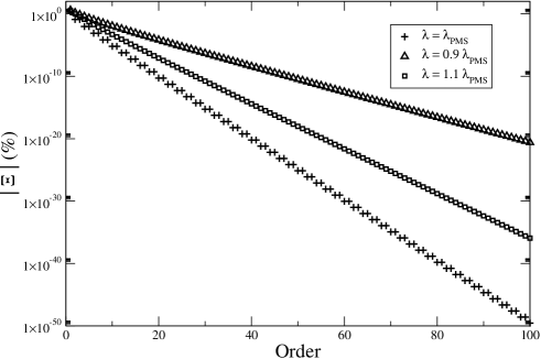
Figure 1: Error over the period (in absolute value), defined as $\Xi\equiv\left[\frac{T_{PMS}-T_{exact}}{T_{exact}}\right]\ \times 100$, for $A=10$ and $\mu=1$ as a function of the order. The three sets are obtained by using the optimal value $\lambda_{PMS}=\sqrt{3\ \mu A^{2}}/2$ (plus), a value $\lambda=0.9\ \lambda_{PMS}$ (triangle) and $\lambda=1.1\ \lambda_{PMS}$ (square).

We consider now the nonlinear pendulum, whose potential is given by $V(\theta)=1-\cos\theta$. By choosing the interpolating potential to be $V_{0}(\theta)=\frac{1+\lambda^{2}}{2}\theta^{2}$ we obtain

$$\Delta(\theta)=-\frac{2}{1+\lambda^{2}}\frac{\cos\Theta-\cos\theta}{\Theta^{2}-\theta^{2}}-1,$$ (14)

where $\Theta$ is the amplitude of the oscillations. To first order our formula yields

$$T_{\delta}=\frac{2\pi}{\sqrt{1+\lambda^{2}}}\Big{(}1+\frac{\delta}{2}\Big{)}-\frac{2\pi\delta}{(1+\lambda^{2})^{3/2}}\frac{J_{1}(\Theta)}{\Theta},$$ (15)

where $J_{1}$ is the Bessel function of the first kind of order 1. The optimal value of $\lambda$ in this case is given by

$$\lambda_{PMS}=\sqrt{\frac{2J_{1}(\Theta)}{\Theta}-1}$$ (16)

and the period to first order is then

$$T_{PMS}=\pi\sqrt{\frac{2\ \Theta}{J_{1}(\Theta)}}.$$ (17)

Despite its simplicity eq. (17) provides an excellent approximation to the exact period over a wide range of amplitudes.

3.2 General Relativity

We now apply our expansion to two problems in General Relativity: the calculation of the deflection of the light by the Sun and the calculation of the precession of a planet orbiting around the Sun. We use the notation of Weinberg [9]:

$$B(r)=A^{-1}(r)=1-\frac{2GM}{r}.$$ (18)

The angle of deflection of the light by the Sun is given by the expression

$$\Delta\phi=2\int_{r_{0}}^{\infty}\sqrt{A(r)}\left[\left(\frac{r}{r_{0}}\right)^{2}\frac{B(r_{0})}{B(r)}-1\right]^{-1/2}\frac{dr}{r}-\pi$$ (19)

where $r_{0}$ is the closest approach.

With the change of variable $z=1/r$ we obtain

$$\Delta\phi=2\ r_{0}^{3/2}\int_{0}^{1/r_{0}}\frac{dz}{\sqrt{r_{0}-r_{0}^{3}z^{2}-2GM(1-r_{0}^{3}z^{3})}}-\pi,$$ (20)

which is exactly in the form of eq. (1). We introduce the potential $V_{0}(z)=(r_{0}^{3}+\lambda^{2})\ z^{2}$ and obtain

$$\Delta(z)=-\frac{\lambda^{2}(z^{2}-\frac{1}{r_{0}^{2}})-2GM\ (1+r_{0}^{3}z^{3})}{(r_{0}^{3}+\lambda^{2})\left(z^{2}-\frac{1}{r_{0}^{2}}\right)}.$$ (21)

By performing the standard steps which are required by our method we obtain the optimal deflection angle to first order to be:

$$\Delta\phi_{PMS}=-\pi+\sqrt{\frac{\pi}{1-\displaystyle\frac{8GM}{r_{0}\pi}}}.$$ (22)

corresponding to the optimal $\lambda$:

$$\lambda_{PMS}^{2}=-\frac{8GMr_{0}^{2}}{\pi}.$$ (23)

The surface corresponding to the closest approach for which $\Delta\phi$ diverges is known as photon sphere and for the Schwartzchild metric takes the value $r_{0}=3GM$. It is remarkable that eq. (23), despite its simplicity, is able to predict a slightly smaller photon sphere, corresponding to $r_{0}=8GM/\pi$. This feature is missed completely in a perturbative approach.

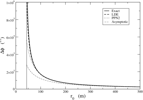
Figure 2: Deflection angle of light obtained assuming $G/c^{2}=7.425\times 10^{-30}\ m/kg$ and $M=1.97\times 10^{30}\ kg$ as function of the closest approach $r_{0}$. The solid line is the exact (numerical) result, the dashed line is obtained with eq. (23), the dotted line is the post-post-Newtonian result of [10], the dot-dashed line is the asymptotic result ($r_{0}\rightarrow\infty$). The vertical line marks the location of the photon sphere, where the deflection angle diverges.

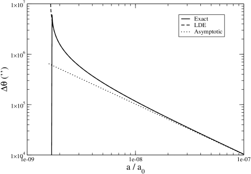
Figure 3: Precession of the orbit of a planet assuming the values $M=1.97\times 10^{30}\ kg$, $G/c^{2}=7.425\times 10^{-30}\ m/kg$ and $\varepsilon=0.2506$ (eccentricity). The scale of reference $a_{0}$ is taken to be the semimajor axis of Mercury’s orbit ($a_{0}=5.971\times 10^{10}\ m$). The solid line is the exact result, the dashed line is the result of eq. (26) and the dotted line is the leading term in the perturbative expansion.

In Figure 2 we compare eq. (23) with the exact numerical result, the post-post-Newtonian (PPN) result of [10] and with the asymptotic result for very small values of $r_{0}$ (close to the photon sphere). We assume $M$ to correspond to the physical mass of the Sun and $G$ to the physical value of the gravitational constant. This corresponds to a strongly nonperturbative regime, where the gravitational force is extremely intense. The reader can judge the quality of our approximation.

We now consider the problem of calculating the precession of the perihelion of a planet orbiting around the Sun. The angular precession is given by [9]

$$\Delta\theta=-2\pi+2\int_{r_{-}}^{r_{+}}\frac{\sqrt{A(r)}\ dr}{r^{2}\sqrt{\displaystyle\frac{1}{J^{2}B(r)}-\frac{E}{J^{2}}-\frac{1}{r^{2}}}}$$ (24)

where $E=\left(\frac{r_{+}^{2}}{B(r_{+})}-\frac{r_{-}^{2}}{B(r_{-})}\right)/\left(r_{+}^{2}-r_{-}^{2}\right)$ and $J^{2}=\left(\frac{1}{B(r_{+})}-\frac{1}{B(r_{-})}\right)/\left(\frac{1}{r_{+}^{2}}-\frac{1}{r_{-}^{2}}\right)$. $r_{\pm}$ are the shortest (perielia) and largest (afelia) distances from the sun. By the change of variable $z=1/r$ we can write eq. (24) as

$$\Delta\theta=-2\int_{z_{-}}^{z_{+}}\frac{1}{\sqrt{(z_{+}-z)(z-z_{-})}}\ \frac{dz}{\sqrt{(1-2GM(z+z_{-}+z_{+}))}}-2\pi,$$ (25)

where $z_{\pm}\equiv 1/r_{\mp}$. Once again the integral has the form required by our method. One obtains

$$\Delta\theta=2\pi\ \\ \left[\frac{\pi(3G^{2}LM^{2}+a(-4L^{2}+48GLM-147G^{2}M^{2}))}{4a(L-6GM)^{2}\sqrt{1-\displaystyle\frac{6\ G\ M}{L}}}-1\right],$$ (26)

where $a$ is the semimajor axis of the ellipse, given by $a\equiv(r_{-}+r_{+})/2$, and $L$ is the semilatus rectum of the ellipse, given by $1/L=(1/r_{+}+1/r_{-})/2$. The optimal $\lambda$ is

$$\lambda_{PMS}=\sqrt{\frac{6GM}{L}}.$$ (27)

In Figure 3 we plot the precession of the orbit calculated through the exact formula (solid line), through eq. (26) (dashed line) and through the leading order result $\Delta\theta_{0}=\frac{6\pi GM}{L}$ (dotted line) [9] . Once again we find excellent agreement with the exact result.

3.3 The spectrum of a quantum potential

In [4] the method described in this paper was applied to the calculation of the spectrum of an anharmonic potential within the WKB method to order $\hbar^{6}$. The WKB condition is

$$\Lambda(E)=\frac{\pi\hbar}{\sqrt{2m}}\ (n+1/2)$$ (28)

where $\Lambda(E)$ to order $O(\hbar^{6})$ is given by

$$\Lambda(E) \equiv {\cal J}_{1}(E)-\frac{\hbar^{2}}{48\ m}\frac{d}{dE}{\cal J}_{2}(E)+\frac{\hbar^{4}}{11520\ m^{2}}\frac{d^{3}}{dE^{3}}{\cal J}_{3}(E)\ .$$ (29)

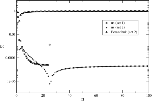
Figure 4: Error over the energy of the anharmonic oscillator with $\hbar=1$, $m=1/2$, $\omega=2$ and $\mu=8000$ (set 1) and with $\hbar=m=\omega=1$ and $\mu=4$ (set 2). The boxes and the pluses have been obtained with our method, the triangles correspond to the error calculated using the analytical formula of [12].

We have defined the integrals:

$${\cal J}_{1}(E) \equiv \int_{x_{-}}^{x_{+}}\sqrt{E-V(x)}dx$$ (30)

$${\cal J}_{2}(E) \equiv \int_{x_{-}}^{x_{+}}\frac{V^{\prime\prime}(x)}{\sqrt{E-V(x)}}dx$$ (31)

$${\cal J}_{3}(E) \equiv \int_{x_{-}}^{x_{+}}\frac{7\ V^{\prime\prime}(x)^{2}-5\ V^{\prime}(x)\ V^{\prime\prime\prime}(x)}{\sqrt{E-V(x)}}dx\ ,$$ (32)

where $x_{\pm}$ are the classical turning points. The spectrum of the potential $V(x)$ can be obtained by solving eq. (29). The integrals appearing in the equations (30), (31) and (32) are of the form required by eq. (1). We can test the method with the quantum anharmonic potential $V(x)=\frac{m\omega^{2}x^{2}}{2}+\frac{\mu x^{4}}{4}$: in [4] it was proved that the integrals above can be analytically approximated with very high precision with our method.

By solving eq. (28) once that the integrals have been approximated with our method one obtaines an analytical formula for the spectrum of the anharmonic oscillator [4]:

$$E_{n} \approx e_{1}\ \left(n+\frac{1}{2}\right)^{\frac{4}{3}}+e_{2}\ \left(n+\frac{1}{2}\right)^{\frac{2}{3}}+e_{3}+\frac{e_{4}}{\left(n+\frac{1}{2}\right)^{2/3}}+\dots$$ (33)

where the first few coefficients $e_{i}$ are given by

$$e_{1} \approx 0.867146\ {\left(\frac{{\mu}\ {{\hbar}}^{4}}{m^{2}}\right)}^{\frac{1}{3}}$$ (34)

$$e_{2} \approx 0.42551\left(\frac{\hbar\ m}{\sqrt{\mu}}\right)^{2/3}\ \omega^{2}$$ (35)

$$e_{3} \approx -0.0466914\ \frac{m^{2}\ \omega^{4}}{\mu}$$ (36)

$$e_{4} \approx 0.030669\left(\frac{\mu\hbar^{4}}{m^{2}}\right)^{1/3}+0.00424238\ \left(\frac{m^{10}\omega^{6}}{\mu^{5}\hbar^{2}}\right)^{1/3}\ .$$ (37)

In Fig. 4 we display the error over the energy defined as $\Sigma\equiv\left|\frac{E_{n}^{(approx)}-E_{n}^{(exact)}}{E_{n}^{(exact)}}\right|\times 100$ as a function of the quantum number $n$. The boxes have been obtained using our formula eq. (33) and assuming $\hbar=1$, $m=1/2$, $\omega=2$ and $\mu=8000$. In this case $E_{n}^{(exact)}$ are the energies of the anharmonic oscillator calculated with high precision in last column of Table III of [11]. The jump corresponding to $n=25$ is due to the low precision of the last value of Table III of [11]. The pluses and the triangles have been obtained using our formula eq. (33) (pluses) and eq. (1.34) of [12] (triangles) and assuming $\hbar=m=\omega=1$ and $\mu=4$. In this case $E_{n}^{(exact)}$ are the energies of the anharmonic oscillator numerically calculated through a fortran code. We can easily appreciate that our formula provides an approximation which is several orders of magnitude better than the one of eq. (1.34) of [12]. We also notice that the formula of [12] yields a quite different asymptotic expansion in the limit of $n\gg 1$. We are not aware of expressions for the spectrum of the anharmonic oscillator similar to the one given by eq. (33).

3.4 The Riemann zeta function

The method outlined above can be applied also to the calculation of the Riemann zeta function [5]. We consider the integral representation

$$\zeta(n) = \frac{(-2)^{n-1}}{2^{n-1}-1}\frac{1}{\Gamma(n)}\int_{0}^{1}\frac{\log^{n-1}x}{1+x}dx\ .$$ (38)

Although eq. (38) is not of the standard form of eq. (2), we can write it as:

$$\zeta(n) = \frac{(-2)^{n-1}}{2^{n-1}-1}\frac{1}{\Gamma(n)}\int_{0}^{1}\frac{1}{1+\lambda}\ \frac{\log^{n-1}x}{1+\frac{x-\lambda}{1+\lambda}}dx,$$ (39)

where $\lambda$ is as usual an arbitrary parameter introduced by hand. In this case $\Delta(x)\equiv\frac{x-\lambda}{1+\lambda}$ and the condition $\left|\frac{x-\lambda}{1+\lambda}\right|<1$ is fullfilled provided that $\lambda>0$; one can expand the denominator in powers of $\frac{x-\lambda}{1+\lambda}$ and obtain:

$$\zeta(n) = \frac{(2)^{n-1}}{2^{n-1}-1}\sum_{k=0}^{\infty}\frac{1}{(1+\lambda)^{k+1}}\sum_{j=0}^{k}\ \frac{k!}{j!(k-j)!}\lambda^{k-j}\frac{(-1)^{j}}{(1+j)^{n}}\ .$$ (40)

Despite its appearance this series does not depend upon $\lambda$, as long as $\lambda>0$. This means that when the sum over $k$ is truncated to a given finite order a residual dependence upon $\lambda$ will survive: such dependence will be minimized by applying the PMS [7], i.e. by asking that the derivative of the partial sum with respect to $\lambda$ vanish. To lowest order one has that $\lambda_{PMS}^{(1)}=2^{-n}$ and the corresponding formula is found:

$$\zeta(n) = \frac{(2)^{n-1}}{2^{n-1}-1}\sum_{k=0}^{\infty}\frac{1}{(1+2^{-n})^{k+1}}\sum_{j=0}^{k}\ \frac{k!}{j!(k-j)!}2^{-n(k-j)}\frac{(-1)^{j}}{(1+j)^{n}}.$$ (41)

We want to stress that eq. (41) is still an exact series representation of the Riemann zeta function. This simple formula yields an excellent approximation to the zeta function even in proximity of $s=1$ where the function diverges. The rate of convergence of the series is greatly improved by applying the PMS to higher orders. In Fig. 5 we plot the difference $|\zeta_{app}(3)-\zeta(3)|$ using eq. (40) with $\lambda=\lambda_{PMS}$ (solid line), $\lambda=0$ (dashed line) and the series representation

$$\zeta(3)=\sum_{n=0}^{\infty}\frac{1}{(n+1)^{3}}$$ (42)

which corresponds to the dotted line in the plot. This last series converges quite slowly and a huge number of terms (of the order of $10^{25}$) is needed to obtain the same accuracy that our series with $\lambda_{PMS}$ reaches with just $10^{2}$ terms. We notice that a special case of eq. (40), corresponding to $\lambda=1$, was already known in the literature [13].

Figure 5: Difference $|\zeta_{app}(3)-\zeta(3)|$ as a function of the number of terms in the sum.

We can extend eq. (40) to the critical line, $s=\frac{1}{2}+i\tau$, and write

$$\zeta\left(\frac{1}{2}+i\tau\right) = \frac{(2)^{-\frac{1}{2}+i\tau}}{2^{-\frac{1}{2}+i\tau}-1}\sum_{k=0}^{\infty}\frac{1}{(1+\lambda)^{k+1}}\sum_{j=0}^{k}\ \frac{k!}{j!(k-j)!}\frac{(-1)^{j}\lambda^{k-j}}{(1+j)^{\frac{1}{2}+i\tau}}$$ (43)

In Fig. 6 we have plotted the error (in percent) over the real part of the zeta function, i.e. $\Xi\equiv Re\left[\frac{\zeta^{(N)}\left(\frac{1}{2}+i\tau\right)-\zeta\left(\frac{1}{2}+i\tau\right)}{\zeta\left(\frac{1}{2}+i\tau\right)}\right]\times 100$, as a function of the number of terms considered in the sum of eq. (43). We use $\tau=50$. The solid line corresponds to the formula of [13], whereas the dashed line corresponds to using our formula, eq. (43), with $\lambda=0.3$.

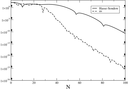
Figure 6: $\Xi\equiv Re\left[\frac{\zeta^{(N)}\left(\frac{1}{2}+i\tau\right)-\zeta\left(\frac{1}{2}+i\tau\right)}{\zeta\left(\frac{1}{2}+i\tau\right)}\right]\times 100$, as a function of the number of terms considered in the sum of eq. (43). The dashed curve is obtained using $\lambda=0.3$.

In Fig. 7 we plot the difference $\zeta^{(\tau)}\left(\frac{1}{2}+i\tau\right)-\zeta\left(\frac{1}{2}+i\tau\right)$ as a function of $\lambda$ for different values of $\tau$. In this case the series is limited to the first $\tau$ terms. The optimal value of $\lambda$ is found close to $\lambda=0.3$.

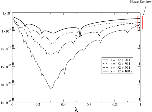
Figure 7: The error obtained using the partial sum of eq. (43) for $s=\frac{1}{2}+i\tau$ and taking the first $\tau$ terms in the sum.

The two figures prove that our expansion is greatly superior to the one of [13].

4 Conclusions

In this paper we have reviewed a method which allows to estimate a certain class of integrals with arbitrary precision. The method is based on the Linear Delta Expansion, i.e. on the powerful idea that a certain (unsoluble) problem can be interpolated with a soluble one, depending upon an arbitrary parameter and then performing a perturbative expansion. The principle of minimal sensitivity allows one to obtain results which converge quite rapidly to the correct results. It is a common occurrence in calculations based on Variational Perturbation Theory, like the present one, that the solution to the PMS equation to high orders cannot be performed analytically. Here, however, we do not face this problem, since we have proved that the method converges in a whole region in the parameter space: the convergence of the expansion is granted as long as the parameter falls in that region.

Although in this paper we have examined a good number of applications of this method to problems both in Physics and Mathematics, we feel that it can be used, with minor modifications, in dealing with many other problems. An extension of the method in this direction is currently in progress.

The author acknowledges support of Conacyt grant no. C01-40633/A-1. He also thanks the organizing comitee of the Dynamical Systems, Control and Applications (DySCA) meeting for the kind invitation to participate to the workshop.

References

• [1] P. Amore and R. A. Sáenz, The Period of a Classical Oscillator, ArXiv:[math-ph/0405030].
• [2] P. Amore, A. Aranda, F. M. Fernández, and R. Sáenz, Systematic Perturbation of Integrals with Applications to Physics, ArXiv:[math-ph/0407014].
• [3] P. Amore and F. M. Fernández, Exact and approximate expressions for the period of anharmonic oscillators, ArXiv:[math-ph/0409034].
• [4] P. Amore and J. Lopez, The spectrum of a quantum potential, ArXiv:[quant-ph/0405090].
• [5] P. Amore, Convergence acceleration of series through a variational approach, ArXiv:[math-ph/0408036].
• [6] A. Okopińska, Phys. Rev. D 35, 1835 (1987); A. Duncan and M. Moshe, Phys. Lett. B 215, 352 (1988)
• [7] P. M. Stevenson, Phys. Rev. D 23, 2916 (1981).
• [8] P. Amore and A. Aranda, Phys. Lett. A 316 218
• [9] S. Weinberg, Gravitation and cosmology, J.Wiley and Sons, 1972
• [10] R. Epstein and I. Shapiro, Phys. Rev. D 22, 2947 (1980); E. Fischbach and B. Freeman, Phys. Rev. D 22, 2950 (1980)
• [11] H. Meissner and O. Steinborn, Phys. Rev. A 56, 1189 (1997).
• [12] I.D. Feranchuk, L.I. Komarov, I.V. Nichipor and A.P. Ulyanenkov, Annals of Physics 238 370 (1995)
• [13] K. Knopp, ”4th Example: The Riemann -Function.” Theory of Functions Parts I and II, Two Volumes Bound as One, Part II. New York: Dover, pp. 51-57, 1996; H. Hasse, ”Ein Summierungsverfahren für die Riemannsche Zeta-Reihe.” Math. Z. 32, 458-464, 1930; J. Sondow, ”Analytic Continuation of Riemann’s Zeta Function and Values at Negative Integers via Euler’s Transformation of Series.” Proc. Amer. Math. Soc. 120, 421-424, 1994.