Dipolar SLEs.

Abstract

We present basic properties of Dipolar SLEs, a new version of stochastic Loewner evolutions (SLE) in which the critical interfaces end randomly on an interval of the boundary of a planar domain. We present a general argument explaining why correlation functions of models of statistical mechanics are expected to be martingales and we give a relation between dipolar SLEs and CFTs. We compute SLE excursion and/or visiting probabilities, including the probability for a point to be on the left/right of the SLE trace or that to be inside the SLE hull. These functions, which turn out to be harmonic, have a simple CFT interpretation. We also present numerical simulations of the ferromagnetic Ising interface that confirm both the probabilistic approach and the CFT mapping.

M. Bauer, D. Bernard and J. Houdayer

Service de Physique Théorique de Saclay

CEA/DSM/SPhT, Unité de recherche associée au CNRS

CEA-Saclay, 91191 Gif-sur-Yvette, France

Two types of stochastic Loewner evolutions (SLE) have been thoroughly studied, the chordal and the radial SLEs [1, 2, 3, 4]. The former describe random curves joining two points on the boundary of a simply connected planar domain while the latter describe curves joining one point on the boundary to a point in the bulk of the domain. They correspond to two inequivalent normalizations of conformal maps between simply connected domains in $\mathbb{C}$. Using geometrical constraints, we realized in ref.[8] that there was a third inequivalent normalization and thus that there was yet another process, which we called the dipolar SLE, with all properties required to define an SLE, depending as usual on a real positive parameter $\kappa$. Concretely, dipolar SLEs describe random curves in a simply connected planar domain which start at a point $x_{0}$ on the boundary and are stopped the first time they hit the boundary on a specified interval $[x_{+},x_{-}]$ not containing $x_{0}$. They generalize chordal SLEs. One of the virtues of dipolar versus chordal SLEs is that the hull does not fill the full domain for $\kappa>4$. This makes the dipolar geometry physically appealing. It is for instance the most natural one to describe several interface properties already computed, such as Cardy’s formula for percolation [5, 6]. The chordal case corresponds to the limit when $x_{+}$ and $x_{-}$ merge together, and in this limit the hull invades the full domain for $\kappa>4$.

The aim of the following is to introduce dipolar SLEs and to present their basic properties.

Section 1 gives the precise definition of dipolar SLEs.

Section 2 is a digression of general nature which emphasizes why (conditional) correlation functions of models of statistical mechanics are martingales for appropriate stochastic processes. This can be used to elucidate the link between SLEs and conformal field theories (CFTs).

Section 3 applies these general ideas to build the CFT interpretation of dipolar SLEs, identifying in particular the boundary operators acting at $x_{0}$ and $x_{\pm}$.

Section 4 is devoted to the computation of some basic dipolar bulk probabilities for $\kappa>4$, namely the probability for a point to be on the left of (resp. on the right of) or swallowed by the SLE hull. These probabilities are computable because they turn out to be harmonic solutions of the general martingale equation (7). Why this equation has interesting harmonic solutions remains to be explained. In fact, the probabilities for a point to be swallowed by the hull from the left or from the right for $\kappa>4$ are non-harmonic, and so are the probabilities to be on the left or on the right of the SLE hull for $\kappa<4$. The explicit computation of these probabilities has eluded us.

Section 5 is devoted to the limiting case $\kappa=4$ and its relation to free field theory with an alternation of appropriate boundary conditions, namely Dirichlet between $x_{-}$ and $x_{0}$, and between $x_{0}$ and $x_{+}$ (but with two different boundary values), and Neumann between $x_{+}$ and $x_{-}$.

In Section 6 we compute, for arbitrary $\kappa$, the distribution of the hitting point of the hull on the interval $[x_{-},x_{+}]$ that does not contain $x_{0}$. We also give a detailed CFT derivation of the result.

In Section 7 we present Monte Carlo simulations of the Ising ferromagnet with specific boundary conditions corresponding to the case $\kappa=3$. The distribution of the interface endpoint agrees very well with the theoretical prediction presented in this article. This confirms the validity of the mapping to the Ising model.

1 Dipolar SLEs.

As for any SLEs, the random curves, often called SLE traces, are encoded into a family of conformal maps $g_{t}(z)$ parameterized by a ‘time’ $t$. When the traces are simple curves, the map $g_{t}$ uniformizes the complement of the portion of the curve $\gamma_{[0,t]}$ in the domain on which the curve is growing back into this domain. Such maps exist by the Riemann mapping theorem and they are defined up to $SL_{2}(\mathbb{R})$ transformations by global conformal symmetry. Thus we need three conditions to fully specify them. For dipolar SLEs, we choose two points on the boundary, $x_{\pm}$, and impose that $g_{t}(x_{\pm})=x_{\pm}$ and $g_{t}^{\prime}(x_{+})=g_{t}^{\prime}(x_{-})$ for each $t$. The process is then defined by specifying the stochastic evolution of $g_{t}$ via a Loewner equation. The dipolar SLE maps describe curves starting at a point $x_{0}\neq x_{\pm}$ on the boundary and ending on the boundary at a random point on the interval between the two fixed points that does not contain $x_{0}$. The crucial point is that for a simply connected domain, the group of conformal automorphisms fixing two boundary points is a one parameter Lie group isomorphic to the additive group of real numbers. Hence, there is a canonical definition of a Brownian motion between $x_{-}$ and $x_{+}$ starting at $x_{0}$, at least when the corresponding boundary interval is a simple curve. See [1, 2, 3, 4] for basic – and not so basic – material on SLEs.

To be more concrete, let $\mathbb{S}_{\Delta}=\{z\in\mathbb{C},\ 0<\Im{\rm m}\,z<\pi\Delta\}$ be the strip of width $\pi\Delta$ which is the geometry adapted to dipolar SLEs. By definition, the dipolar Loewner equation in $\mathbb{S}_{\Delta}$ reads:

$$\partial_{t}g_{t}(z)=\frac{1/\Delta}{\tanh\left({(g_{t}(z)-\xi_{t})/2\Delta}\right)},\quad g_{t=0}(z)=z,$$ (1)

with $\xi_{t}=\sqrt{\kappa}\,B_{t}$ with $B_{t}$ a normalized Brownian motion and $\kappa$ a real positive parameter so that ${\bf E}[\xi_{t}\,\xi_{s}]=\kappa\,{\rm min}(t,s)$. The two boundary fixed points are $x_{\pm}=\pm\infty$ and the starting point $x_{0}$ is the origin. The maps $g_{t}$ are normalized to fix $x_{\pm}$. For fixed $z$, $g_{t}(z)$ is well-defined up to the time $\tau_{z}$ for which $g_{\tau_{z}}(z)=\xi_{\tau_{z}}$. Times $\tau_{z}$ are called swallowing times. In the limit $\Delta\to\infty$ we recover the chordal SLEs. $\Delta$ is simply a dilatation factor. Unless otherwise specified, we will set $\Delta=1$ in the following and we will look at dipolar SLEs in the strip $\mathbb{S}_{1}$.

As for chordal or radial SLEs [1, 2, 3, 4], the SLE hull is reconstructed from $g_{t}$ by $\mathbb{K}_{t}=\{z\ \mathrm{such~{}that}\ \tau_{z}\leq t\}$ and the SLE trace $\gamma_{[0,t]}$ by $\gamma(t)=\lim_{\epsilon\to 0^{+}}g_{t}^{-1}(\xi_{t}+i\epsilon)$. It is known that $\gamma_{[0,t]}$ is almost surely a curve. It is non-self intersecting and it coincides with $\mathbb{K}_{t}$ for $0<\kappa\leq 4$, while for $4<\kappa<8$ it possesses double-points and it does not coincide with $\mathbb{K}_{t}$ which is then the set of points swallowed up to time $t$. For $\kappa\geq 8$, the trace is space filling. However, in contrast to the chordal SLE case, for dipolar SLEs, the hull does not fill the entire domain even for $\kappa\geq 8$.

It will be convenient to consider the map which maps the tip of the SLE trace back to its starting point. Thus we translate $g_{t}$ and let $f_{t}(z)=g_{t}(z)-\xi_{t}$ so that $f_{t}(\gamma(t))=0$. The dipolar stochastic equation is simply:

$$df_{t}(z)=\Delta^{-1}\,\coth(f_{t}(z)/2\Delta)+d\xi_{t}.$$

The maps $f_{t}$ are such that, for $s>t$, $f_{s}\circ f_{t}^{-1}$ is distributed as $f_{s-t}$.

Eq.(1) may be integrated in the simple deterministic case with $\xi_{t}$ constant. Then $\cosh(g_{t}(z)-\xi)/2=e^{t/2}\,\cosh(z-\xi)/2$ for $\Delta=1$. The trace $\gamma(t)$ is determined by $\cosh(\gamma(t)-\xi)/2=e^{-t/2}$, so that it starts on the real axis at $\xi$ and stops when it touches the upper boundary of the strip at the point $i\pi+\xi$. As expected, all points at the left of the trace are mapped to the fixed point at $-\infty$ by $f_{t}$ as $t\to\infty$, while those on the right of the curve are mapped into the other fixed point $+\infty$.

Let us return to the case when $\xi_{t}$ is a Brownian motion. A simple probabilistic argument, explained in [8], shows that the probabilities for the trace to touch the upper boundary in finite time vanishes. So, the trace only touches this boundary at infinite time. This amounts to stop the process when the trace hits the upper boundary, a criterion which is invariant under time reparametrizations of the evolution. Since locally the dipolar SLE trace looks the same as the chordal or radial SLE traces [2], this leads to the following picture. For $\kappa\leq 4$, the hull coincides with the trace. The latter does not touch the lower boundary, ie. the real axis $\mathbb{R}$, but stops when it hits the upper boundary, ie. $i\pi+\mathbb{R}$, at same random point. For $\kappa>4$, the trace is not a simple curve and points in $\mathbb{S}_{1}$ are swallowed, the set of which form the SLE hull. The hull then intersects the lower boundary, ie. the real axis, and the trace hits this boundary an infinite number of times but hits only once the upper boundary, again at some random point, and stops there. See Figure (1).

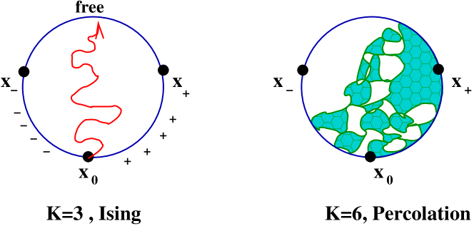
Figure 1: Two schematic examples of dipolar SLEs.

2 Statistical mechanics and martingales.

This section is a recreative interlude in which we explain why (conditional) correlation functions of models of statistical mechanics are martingales for appropriate stochastic processes. As a very general statement this remark may look tautological but it is nevertheless quite instructive. In particular it provides a key to decipher the relation between SLEs and CFTs.

Let ${\cal C}$ be the configuration space of a statistical model. For simplicity we assume ${\cal C}$ to be discrete and finite but as large as desired. Let $W_{c}$ be the Boltzmann weights and $Z$ the partition function, $Z=\sum_{c\in{\cal C}}\ W_{c}$.

We imagine having introduced a family ${\cal Q}_{t}$ of partitions of the configuration space whose elements ${\cal C}_{\alpha_{t}}$ are labeled by indices $\alpha_{t}$:

$${\cal C}=\bigcup_{\alpha_{t}}{\cal C}_{\alpha_{t}},\qquad{\cal C}_{\alpha_{t}}\ {\rm disjoints}.$$

The index $t$, which will be identified with ‘time’, labels the partitions. By convention ${\cal Q}_{0}$ is the trivial partition with ${\cal C}$ as its single piece. We assume these partitions to be finer as $t$ increases, which means that for any $s>t$ and any element ${\cal C}_{\alpha_{t}}$ of the partition at time $t$ there exist elements of ${\cal Q}_{s}$ which form a partition of ${\cal C}_{\alpha_{t}}$. An example of such partitions in case of spin statistical models consists in specifying the values of local spin variables at an increasing number of lattice points. Block spin clustering used in renormalization group is another way to produce such partitions. A SLE inspired example consists in specifying the shapes and the positions of interfaces of increasing lengths.

We define the restricted partition function $Z_{\alpha_{t}}$ by

$$Z_{\alpha_{t}}\equiv\sum_{c\in{\cal C}_{\alpha_{t}}}W_{c}~{}.$$

Since restricting the summation to a subset amounts to impose some condition on the statistical configurations, $Z_{\alpha_{t}}$ is the partition function conditioned by the knowledge specified by ${\cal C}_{\alpha_{t}}$.

To define a stochastic process we have to specify the probability space and a filtration on it. The simplest choice is ${\cal C}$ as a probability space equipped with its canonical $\sigma$-algebra, ie. the one generated by all its singletons, and with the probability measure induced by the Boltzmann weights, ie. ${\bf P}[\{c\}]=W_{c}/Z$. In particular the probability of the event ${\cal C}_{\alpha_{t}}$ is the ratio of the partition functions

$${\bf P}[{\cal C}_{\alpha_{t}}]=Z_{\alpha_{t}}/Z.$$

To any partition ${\cal Q}_{t}$ is associated a $\sigma$-algebra on ${\cal C}$, ie. the one generated by the elements of this partition. Since these partitions are finer as ‘time’ $t$ increases, it induces a filtration ${\cal F}_{t}$ on ${\cal C}$ equipped with its probability measure.

Now, given an observable ${\cal O}$ of the statistical model, ie. a function $c\to{\cal O}_{c}$ on the configuration space, we can define its conditional average

$$\langle{\cal O}\rangle_{t}\equiv{\bf E}[{\cal O}|{\cal F}_{t}].$$

By construction, $\langle{\cal O}\rangle_{t}$ is a function which is constant on any element ${\cal C}_{\alpha_{t}}$ of the partition ${\cal Q}_{t}$ and takes values

$$\langle{\cal O}\rangle_{t}|_{{\cal C}_{\alpha_{t}}}=\frac{1}{Z_{\alpha_{t}}}\sum_{c\in{\cal C}_{\alpha_{t}}}{\cal O}_{c}\ W_{c}.$$

This is simply the statistical average conditioned on the knowledge specified by ${\cal C}_{\alpha_{t}}$.

By construction, $\langle{\cal O}\rangle_{t}$ is a (closed) martingale with respect to ${\cal F}_{t}$. Indeed, for $t>s$,

$${\bf E}[\langle{\cal O}\rangle_{t}|{\cal F}_{s}]={\bf E}[{\bf E}[{\cal O}|{\cal F}_{t}]|{\cal F}_{s}]={\bf E}[{\cal O}|{\cal F}_{s}]=\langle{\cal O}\rangle_{s},$$

where we used standard properties of conditional expectations and that ${\cal F}_{t}\subset{\cal F}_{s}$ for $t>s$. In particular, one may verify that its average is time independent and equals to the statistical average:

$${\bf E}[\langle{\cal O}\rangle_{t}] = \sum_{\alpha_{t}}{\bf P}[{\cal C}_{\alpha_{t}}]\ \langle{\cal O}\rangle_{t}|_{{\cal C}_{\alpha_{t}}}$$

$$= \frac{1}{Z}\sum_{c\in{\cal C}}{\cal O}_{c}\ W_{c}=\langle{\cal O}\rangle.$$

This observation formally applies to critical interfaces and hence to SLEs. The remarkable observation made by O. Schramm is that conformal invariance implies that the filtration associated to the partial knowledge of the interface is that of a continuous martingale, i.e. that of a Brownian motion if time is chosen cleverly. The only parameter is $\kappa$. The physical parameters of the CFT, for instance the central charge, can be retrieved by imposing that the correlation functions $\langle{\cal O}\rangle_{t}$ conditioned by the knowledge of ${\cal F}_{t}$ be martingales. The CFT situation is particularly favorable in that going from $\langle{\cal O}\rangle_{t}$ to $\langle{\cal O}\rangle$ is pure kinematics.

3 CFT connections.

Connection with conformal field theories can be done using the CFT operator formalism. The latter is simpler if the boundary CFT is considered in the upper half plane $\mathbb{H}=\{z\in\mathbb{C},\Im{\rm m}\,z>0\}$.

SLE processes are transported onto any simply connected domain by conformal transformations, by definition. In $\mathbb{H}$, we fix the boundary points $x_{\pm}$ to be $\pm 1$ and $x_{0}$ to be the origin. The conformal map uniformizing $\mathbb{S}_{\Delta}$ onto $\mathbb{H}$ is $\varphi(w)=\tanh(w/2\Delta)$. Let $\hat{g}_{t}$ be the dipolar SLE map in $\mathbb{H}$, $\hat{g}_{t}\circ\varphi=\varphi\circ g_{t}$. The stochastic Loewner equation for dipolar SLE in $\mathbb{H}$ reads [8]:

$$\partial_{t}\hat{g}_{t}(z)=\left(\frac{1-\hat{g}_{t}(z)^{2}}{2}\right)\,\left(\frac{1-\hat{g}_{t}(z)\tanh\xi_{t}/2}{\hat{g}_{t}(z)-\tanh\xi_{t}/2}\right),\quad\hat{g}_{t=0}(z)=z.$$

The maps $\hat{g}_{t}$ are normalized to fix $x_{\pm}=\pm 1$ and to have equal derivatives at these two points : $\hat{g}^{\prime}_{t}(\pm 1)=e^{-t}$.

The map $f_{t}$ can also be transported in the upper half plane to produce a map $\hat{f}_{t}=\tanh(f_{t}/2\Delta)$, which also fixes $x_{\pm}=\pm 1$ but which maps the tip of the SLE trace in $\mathbb{H}$ to the origin. Its expression is:

$$\hat{f}_{t}(z)=\frac{\hat{g}_{t}(z)-\tanh\xi_{t}/2}{1-\hat{g}_{t}(z)\tanh\xi_{t}/2}.$$

The stochastic differential equation that $\hat{f}_{t}$ satisfies directly follows from that obeyed by $f_{t}$.

As for the chordal and radial cases [7], the connection between SLEs and CFTs may be established by associating to $\hat{f}_{t}$ an operator $\hat{G}_{t}$ which implements this conformal transformation in the CFT Hilbert space. Since $\hat{f}_{t}$ fixes the point $x_{+}$, or $x_{-}$, $\hat{G}_{t}$ may be constructed as an element of the enveloping algebra of the appropriate Borel sub-algebra of the Virasoro algebra. See [7] for details. It intertwines between primary fields, say $\Phi_{h,\bar{h}}(z,\bar{z})$ of conformal dimensions $(h,\bar{h})$, and their images under $\hat{f}_{t}$. Namely,

$$\hat{G}_{t}^{-1}\,\Phi_{h,\bar{h}}(z,\bar{z})\,\hat{G}_{t}=[\hat{f}_{t}^{\prime}(z)]^{h}[\overline{\hat{f}_{t}^{\prime}(z)}]^{\bar{h}}\ \Phi_{h,\bar{h}}(\hat{f}_{t}(z),\overline{\hat{f}_{t}(z)}).$$

The stochastic differential equation that $\hat{G}_{t}$ satisfies directly follows from that of $\hat{f}_{t}$, or $\hat{g}_{t}$. It reads [8]:

$$\hat{G}_{t}^{-1}\,d\hat{G}_{t}=(-2W_{-2}+\frac{\kappa}{2}W_{-1}^{2})dt-W_{-1}d\xi_{t},$$ (2)

where $W_{-2}$ and $W_{-1}$ are elements of the Virasoro algebra,

$$W_{-2}=\frac{1}{4}(L_{-2}-L_{0}),\quad W_{-1}=\frac{1}{2}(L_{-1}-L_{1}).$$

In this algebraic setting, the differences between radial and dipolar SLEs may be viewed as coming from a different choice of real forms in the Virasoro algebra.

As in the chordal and radial SLEs, the key point is now the construction of a generating function of local martingales which is obtained using a representation of the Virasoro algebra degenerate at level two.

Let $|\omega\rangle$ be the highest weight vector of the irreducible Virasoro module with central charge $c$ and conformal weight $h_{1;2}$,

$$c=\frac{(\kappa-6)(8-3\kappa)}{2\kappa},\quad h_{1;2}=\frac{6-\kappa}{2\kappa},$$

then

$$M_{t}\equiv e^{+2h_{0;1/2}\,t}\,\hat{G}_{t}|\omega\rangle$$ (3)

is a local martingale, with

$$h_{0;1/2}=\frac{(6-\kappa)(\kappa-2)}{16\kappa}.$$

This follows from the null vector relation $(-2L_{-2}+\frac{\kappa}{2}L_{-1}^{2})|\omega\rangle=0$. Indeed, a simple rearrangement leads to

$$-2W_{-2}+\frac{\kappa}{2}W_{-1}^{2}=\frac{1}{4}(-2L_{-2}+\frac{\kappa}{2}L_{-1}^{2})+\frac{2-\kappa}{4}L_{0}+\frac{\kappa}{8}(L_{1}^{2}-2L_{-1}L_{1}),$$

so that $(-2W_{-2}+\frac{\kappa}{2}W_{-1}^{2})|\omega\rangle=-2h_{0;1/2}|\omega\rangle$ and

$$\hat{G}^{-1}d\hat{G}_{t}|\omega\rangle=-dt\,2h_{0;1/2}|\omega\rangle+d\xi_{t}\,W_{-1}|\omega\rangle.$$

In particular, by projecting this local martingale on vectors $\langle v|$ and assuming appropriate boundedness conditions, we get that the expectations ${\bf E}[e^{2h_{0;1/2}t}\,\langle v|\hat{G}_{t}|\omega\rangle]$ are time independent.

The prefactor $e^{+2h_{0;1/2}t}$ accounts for the insertion of two boundary conformal fields, each of dimension $h_{0;1/2}$, localized at the two fixed points $x_{\pm}$ since $\hat{f}_{t}^{\prime}(x_{+})\hat{f}_{t}^{\prime}(x_{-})=e^{-2t}$. Alternatively, the local martingales can be written as the ratio of two correlation functions with insertions of the boundary operator $\psi_{1;2}$ creating the state $|\omega\rangle$ at $x_{0}$ and of the operators $\psi_{0;1/2}$ at the fixed points $x_{\pm}$:

$$\frac{\langle\psi_{0;1/2}(x_{-})\psi_{0;1/2}(x_{+})\,{\cal O}\,\hat{G}_{t}\,\psi_{1;2}(x_{0})\rangle}{\langle\psi_{0;1/2}(x_{-})\psi_{0;1/2}(x_{+})\,\hat{G}_{t}\,\psi_{1;2}(x_{0})\rangle}$$ (4)

for any operator ${\cal O}$. Since martingales are key ingredients for computing probabilities, this statement implies that dipolar SLE probabilities will be expressible in terms of CFT correlation functions with insertions of these boundary operators.

By conformal invariance, this last expression can be transported to any simply connected planar domain $\mathbb{S}$. If $g_{t}$ is the conformal map describing the growth of the dipolar SLE hulls in $\mathbb{S}$, mapping the tip of the SLE trace to $x_{0}\in\partial\mathbb{S}$, then the ratios

$$\frac{\langle\psi_{0;1/2}^{g_{t}}(x_{-})\psi_{0;1/2}^{g_{t}}(x_{+})\,{\cal O}^{g_{t}}\,\psi_{1;2}(x_{0})\rangle}{\langle\psi_{0;1/2}^{g_{t}}(x_{-})\psi_{0;1/2}^{g_{t}}(x_{+})\psi_{1;2}(x_{0})\rangle}$$ (5)

are local martingales. Here $\psi^{g_{t}}_{0;1/2}$, $\psi^{g_{t}}_{1;2}$ or ${\cal O}^{g_{t}}$ denote the images of the corresponding fields by $g_{t}$, ie. their pull-back by $g_{t}$. As explained in the previous section, this statement has a natural explanation in basic statistical mechanics. Although this construction can be seen merely as a trick to construct martingales, the previous section explains why the martingale property is what ensures that the CFT identified in this way is precisely the critical continuum limit of the statistical mechanics model that produces the interface described by SLE.

— Examples:

Dipolar SLEs has a simple statistical interpretation for $\kappa=3$ which corresponds to the Ising model with $c=1/2$. Then $\psi_{1;2}$ with $h_{1;2}=1/2$ is the boundary condition changing operator between spin $(+)$ and spin $(-)$ fixed boundary conditions, while $\psi_{0;1/2}$ with $h_{0;1/2}=1/16$ is the boundary condition changing operator between fixed and free boundary conditions [9]. Hence, along the boundary of the domain one encounters the boundary conditions fixed $(+)$, then free, and then again fixed but $(-)$, as depicted in Fig.(1). It is thus clear that we need one operator $\psi_{1;2}$ and two operators $\psi_{0;1/2}$ to describe this system.

As we shall see in the following sections, the case $\kappa=4$ which corresponds to a free bosonic field with $c=1$ also has a simple interpretation with an alternation of Dirichlet and Neumann boundary conditions.

For the 3-state Potts model we may propose the following interpretation. The microscopic spin variables take three possible values $(1)$, $(2)$ and $(3)$ related by $S_{3}$ symmetry. The 3-state Potts model corresponds to $\kappa=10/3$ with central charge $c=4/5$. Then $h_{1;2}=2/5$ and $h_{0;1/2}=1/15$. The operator $\psi_{1;2}$ is the boundary operator between a fixed boundary condition with all spins $(1)$ and a mixed boundary condition $(2+3)$ with a mixture of spins $(2)$ and $(3)$. The operator $\psi_{0;1/2}$ is the boundary operator between the boundary conditions $(1)$ and $(1+2)$. It is also the lowest boundary primary operator generated by a change of mixed boundary conditions from $(1+2)$ to $(2+3)$, see ref.[9]. Thus the dipolar SLE with $\kappa=10/3$ should correspond to the 3-Potts models with the succession of boundary conditions, fixed $(1)$, mixed $(2+3)$ and mixed $(1+2)$.

Unitary minimal CFTs with $c=1-6/m(m+1)$ with $m$ integer correspond to two values of $\kappa$ related by duality: $\kappa=4(m+1)/m$ or $\kappa=4m/(m+1)$. Since the identification of $\psi_{0;1/2}$ depend on the parity of $m$ — ie. $h_{0;1/2}=h_{m/2;m/2}$ for $m$ even, $\kappa\geq 4$, but $h_{0;1/2}=h_{(m+1)/2;(m+1)/2}$ for $m$ odd, $\kappa\leq 4$, — a simple microscopic interpretation is possible only for one of the two choices of $\kappa$. For instance, although $\kappa=16/3$ corresponds to the Ising model, the role of the Virasoro representation with weight $h_{0;1/2}=5/192$ in the Ising model has not yet been clearly identified.

4 Bulk visiting probabilities and harmonic functions ($\kappa>4$).

Let us now look at SLE bulk properties. We assume $\kappa>4$ and we deal with dipolar SLEs in the strip $\mathbb{S}_{1}$. We shall evaluate the following probabilities:

(i) The probabilities $P_{l}(z,\bar{z})$ (resp. $P_{r}(z,\bar{z})$) for a bulk point $z$ not to be swallowed by the SLE trace and to be on the left (resp. the right) of the trace. This is the probability for the point $z$ to be on the left (resp. the right) of the exterior frontier of the SLE hull viewed from the boundary point $x_{-}$ (resp. $x_{+}$). It is therefore the probability for the existence of a path joining $x_{-}$ (resp. $x_{+}$) to the boundary interval $[x_{+},x_{-}]$ leaving the point $z$ on its right (resp. left) and included into one cluster of the underlying model of statistical mechanics. For $\kappa=6$ it bears some similarities with the probability computed by Smirnov [6] to prove the equivalence between critical percolation and $SLE_{6}$.

(ii) The probability $P_{in}(z,\bar{z})$ for the point $z$ to be in the SLE hull. We do not distinguish the events in which the point has been swallowed from the right or from the left. Since this probability is also that for the point $z$ to be in left or right frontiers of the hull it gives informations on the shape of the hull. These probabilities turn out to be harmonic functions for all values of $\kappa>4$ and are proportional to the CFT correlation functions

$$\langle\psi_{0;1/2}(x_{-})\psi_{0;1/2}(x_{+})\Phi_{0}(z,\bar{z})\psi_{1;2}(x_{0})\rangle$$ (6)

involving a weight zero bulk primary field $\Phi_{0}$.

As usual, a way to compute these probabilities is to notice that the process $t\to P(f_{t}(z),\overline{f_{t}(z)})$ is a local martingale. Indeed, since $f_{s}\circ f_{t}^{-1}$, $s>t$, is independent of $f_{t}$ and distributed as $f_{s-t}$, the function $P(f_{t}(z),\overline{f_{t}(z)})$ is the probability of the events (i), or (ii), conditioned on the process up to time $t$ and, as such, it is a martingale. As a consequence, the drift term in the Itô derivative of $P(f_{t}(z),\overline{f_{t}(z)})$ vanishes which implies that $P(z,\bar{z})$ satisfies the following differential equation:

$$\kappa\partial_{z}\bar{\partial}_{\bar{z}}P+(\coth\frac{z}{2}+\frac{\kappa}{2}\partial_{z})\partial_{z}P+(\coth\frac{\bar{z}}{2}+\frac{\kappa}{2}\partial_{\bar{z}})\partial_{\bar{z}}P=0.$$ (7)

The main observation in this section is that, quite remarkably, eq.(7) has interesting harmonic solutions, in fact enough harmonic solutions to compute $P_{l}$, $P_{r}$ and $P_{in}$.

The boundary conditions depend on which probabilities we are computing:
(i) For the probability to be on the left of the hull, this requires:

$$P_{l}(-\infty)=1,\quad P_{l}(+\infty)=0,\quad P_{l}(0)=0.$$ (8)

Similar conditions hold for $P_{r}(z,\bar{z})$.
(ii) For the probability to be in the hull, it requires:

$$P_{in}(-\infty)=P_{in}(+\infty)=0,\quad P_{in}(0)=1.$$ (9)

These boundary conditions follow by noticing that if point $z$ is swallowed at time $\tau_{z}$ then $\lim_{t\nearrow\tau_{z}}f_{t}(z)=0$, if it is not swallowed but is on the left of the trace then $\lim_{t\nearrow\infty}f_{t}(z)=-\infty$, and if it is not swallowed but is on the right of the trace then $\lim_{t\nearrow\infty}f_{t}(z)=+\infty$. These conditions are such that at the stopping $\widehat{\tau}_{z}={\rm min}(\tau_{z},\infty)$ the martingale $P(f_{t}(z),\overline{f_{t}(z)})$ projects on the appropriate events (i) or (ii), ie. $P(f_{\widehat{\tau}_{z}}(z),\overline{f_{\widehat{\tau}_{z}}(z)})={\bf 1}_{{\rm events}}$. As a consequence, the probability of these events are:

$${\bf P}[{\rm events}]\equiv{\bf E}[{\bf 1}_{{\rm events}}]={\bf E}[P(f_{\widehat{\tau}_{z}}(z),\bar{f}_{\widehat{\tau}_{z}}(z))]=P(z,\bar{z}).$$

The martingale property has been used in the last equality.

— Case (i): probability to be on the left of the trace.

The solution of the martingale equation (7) satisfying the boundary conditions (8) is given by the harmonic function

$$P_{l}(z,\bar{z})=1-\frac{\Im{\rm m}\,F(z)}{\Im{\rm m}\,F(\infty)}$$ (10)

with

$$F(z)\equiv\int_{-\infty}^{z}\frac{du}{(\sinh u/2)^{4/\kappa}}.$$

The function $F(z)$ is well-defined and analytic on the strip $\mathbb{S}_{1}$ for all $\kappa$’s. For $\kappa>4$, $F(z)$ is bounded and has a continuous extension to the closure of $\mathbb{S}_{1}$. For $\kappa<4$, it is unbounded near the origin and so are the corresponding solutions to eq.(7). In that case these solutions only lead to local martingales and not true martingales. See Appendix for details on its definition and on its properties. We have $\Im{\rm m}\,F(\infty)=-\sin(2\pi/\kappa))\,I=-\sin(4\pi/\kappa))\,J$ with

$$I=\int_{-\infty}^{+\infty}dy(\cosh y/2)^{-4/\kappa},\qquad J=\int_{0}^{\infty}dy(\sinh y/2)^{-4/\kappa}.$$

As a check one may verify that $P_{l}(z,\bar{z})$ behaves as expected on the boundary. On the positive real axis, $(\sinh z/2)$ is real and positive so that

$$P_{l}(x)=0,\quad x\in\mathbb{R}_{+},$$

in accordance with the fact that no point on the real axis can be on the left of the trace. On the negative real axis, $(\sinh x/2)^{4/\kappa}=e^{i4\pi/\kappa}(\sinh|x|/2)^{4/\kappa}$ and

$$P_{l}(x)=1-\frac{1}{J}\int_{|x|}^{+\infty}\frac{dy}{(\sinh y/2)^{4/\kappa}},\quad x\in\mathbb{R}_{-},$$

which interpolates between one and zero. It gives the probability of the hull not to spread further than $x$ on the negative real axis. On the upper boundary,

$$P_{l}(z=i\pi+x)=1-\frac{1}{I}\int_{-\infty}^{x}\frac{dy}{(\cosh y/2)^{4/\kappa}},\quad z\in i\pi+\mathbb{R},$$

since there $(\sinh z/2)^{4/\kappa}=e^{2i\pi/\kappa}(\cosh x/2)^{4/\kappa}$. This yields the density probability for the trace to stops on an interval $[x,x+dx]$ on the upper boundary.

— Case (ii): probability to be inside the hull.

The solution of the martingale equation (7) satisfying the boundary conditions (9) is given by the harmonic function

$$P_{in}(z,\bar{z})=\frac{\Im{\rm m}[e^{i2\pi/\kappa}\,F(z)\,]}{\Im{\rm m}[e^{i2\pi/\kappa}\,F(0)\,]}$$ (11)

with identical function $F(z)$ as above and $\Im{\rm m}[e^{i2\pi/\kappa}\,F(0)\,]=-\sin(2\pi/\kappa)\,J$. Again, $P_{in}$ has the expected behavior on the boundary. Since $e^{i2\pi/\kappa}\,F(z)$ is real on the upper boundary, we have

$$P_{in}(z,\bar{z})=0,\quad z\in i\pi+\mathbb{R},$$

in agreement with the fact that no point on the upper boundary can be swallowed. $P_{in}$ is even on the real axis and

$$P_{in}(x)=\frac{1}{J}\int_{|x|}^{+\infty}\frac{dy}{(\sinh y/2)^{4/\kappa}},\quad x\in\mathbb{R}.$$

This is of course complementary to $P_{l}(x)$ for $x$ negative.

— CFT interpretation.

The correlation function (6) has a natural interpretation in the Coulomb gas representation of CFTs: the weight zero primary field $\Phi_{0}$ is simply the integral of the screening current. Recall that CFT with $c=1-12\alpha_{0}^{2}<1$ may be represented in terms of a free bosonic field $\varphi(z)$ with a background charge $2\alpha_{0}$, see refs.[10, 11, 12]. The conformal weight of a state of coulomb charge $\alpha$, or $2\alpha_{0}-\alpha$, is $h(\alpha)=\frac{1}{2}\alpha(\alpha-2\alpha_{0})$. The weight $h_{r;s}={[(r\kappa-4s)^{2}-(\kappa-4)^{2}]}/{16\kappa}$ corresponds to the charge $\alpha_{r,s}=\alpha_{0}-\frac{r}{2}\alpha_{+}-\frac{s}{2}\alpha_{-}$ with $\alpha_{\pm}$ the two screening charges. In the present case $c=1-6{(\kappa-4)^{2}}/{4\kappa}$ and the correspondence is $\alpha_{-}=-2\sqrt{2/\kappa}$, $\alpha_{+}=\sqrt{\kappa/2}$ and $2\alpha_{0}=\alpha_{+}+\alpha_{-}$. In particular $\alpha_{1;2}=-\alpha_{-}/2$ and $\alpha_{0;1/2}=\alpha_{0}\pm\alpha_{-}/4$. The screening charges are such that the currents $Q_{\pm}(z)=\exp(i\alpha_{\pm}\varphi(z))$ have weight one. The operator $\Phi_{0}$ in eq.(6) is a linear combination of the primitive of the screening current $Q_{-}$ and the identity operator, ie:

$$\Phi_{0}(z,\bar{z})={\rm const^{\prime}.}\,{\bf 1}+\Re{\rm e}\,[\,{\rm const.}\,\int^{z}dw\,Q_{-}(w)\,].$$

Indeed this operator has conformal weight zero, satisfies the appropriate fusion rules and fulfills the charge conservation requirement which demands that the sum of the coulomb charges of the operators involve in the correlation function minus the background charge belongs to the lattice generated by the screening charges.

5 The limiting case $\kappa=4$.

For $\kappa=4$ the SLE trace is a simple curve so that no point are swallowed and $P_{in}=0$ for all points. This case is marginal in the sense that the integral defining $F(z)$ is only logarithmically divergent. By extension, we have:

$$P_{l}(z,\bar{z})=\frac{1}{\pi}\Im{\rm m}\,\left[\log(\tanh\frac{z}{4})\right].$$ (12)

This satisfies the martingale equation (7) for $\kappa=4$ and the appropriate boundary conditions: $P_{l}(x\in\mathbb{R}_{+})=0$ and $P_{l}(x\in\mathbb{R}_{-})=1$. Contrary to the cases $\kappa<4$, it is discontinuous at the origin. On the upper boundary the distribution of the trace is given by:

$$P_{l}(i\pi+x)=1-\frac{2}{\pi}\arctan(e^{x/2}),\quad x\in\mathbb{R}.$$

For $\kappa=4$, the Virasoro central charge is $c=1$ and $h_{1;2}=1/4$ and $h_{0;1/2}=1/16$. The probability (12) possesses a nice free field CFT interpretation. Central charge $c=1$ corresponds to bosonic free field. Let us denote by $X$ this field. $h_{1;2}=1/4$ is the conformal weight of the boundary vertex operator $V_{1;2}=\cos X/\sqrt{2}$ which may be thought of as the boundary condition changing operator intertwining two boundary intervals on which two different Dirichlet boundary conditions are imposed. $h_{0;1/2}=1/16$ is the dimension of the twist field $\sigma$ which is the boundary condition changing operator intertwining between Dirichlet and Neumann boundary conditions. Thus the probability $P_{l}(z,\bar{z})$ is proportional to

$$\langle X(z,\bar{z})\rangle_{D;D;N}=\langle\sigma(x_{+})\sigma(x_{-})X(z,\bar{z})V_{1;2}(x_{0})\rangle,$$

where ’D;D;N’ refers to Dirichlet boundary conditions on the lower boundary $[x_{-},x_{0}]$ and $[x_{0},x_{+}]$, but with a discontinuity at $x_{0}$ (ie. two D-branes at finite distance), and Neumann boundary condition on the upper boundary $[x_{-},x_{+}]$ (ie. a space filling brane). The fact $P_{l}(z,\bar{z})$ satisfies the Dirichlet boundary conditions on the lower boundary is clear by construction but one may verify that it actually satisfies the Neumann boundary condition on the upper boundary. The fact that it is a harmonic function is then a consequence of the free field equation of $X$.

6 Boundary excursion probabilities (all $\kappa$’s).

The computations of previous sections yield the density probability of the hitting point on the upper boundary for $\kappa>4$. We now would like to show that this formula actually applies to any value of $\kappa$. So we look for the probability $P_{up}(\hat{x})$, $\hat{x}\in i\pi+\mathbb{R}$, that the SLE trace hits the upper boundary at a point $\hat{u}\equiv i\pi+u$, $u>x$, on the right of $\hat{x}\equiv i\pi+x$. By definition, this probability satisfies:

$$P_{up}(-\infty)=1,\quad P_{up}(+\infty)=0.$$

To change gear we shall do the computation using conformal field theory techniques. Using the CFT martingales (3), or equivalently (5), we aim at proving that this probability is given by the correlation function

$$\langle\psi_{0;1/2}(x_{-})\psi_{0;1/2}(x_{+})\psi_{0}(\hat{x})\psi_{1;2}(x_{0})\rangle,$$

where $\psi_{0}(\hat{x})$ is a weight zero boundary conformal field inserted on the upper boundary. Recall that in the strip geometry $x_{\pm}=\pm\infty$ and $x_{0}=0$. Due to CFT fusion rules, there are two possible choices for $\psi_{0}$ : either it is the identity operator or it is the intertwiner between the Virasoro modules of weights $h_{1;2}=\frac{6-\kappa}{2\kappa}$ and $h_{1;0}=\frac{\kappa-2}{2\kappa}$. The existence of two choices makes possible to fulfill the above two boundary conditions. These boundary condition code for the behavior of the functions as $\hat{x}$ approaches $x_{-}$ or $x_{+}$. In CFT correlation functions this behavior is governed by fusing $\psi_{0}$ with $\psi_{0;1/2}$. In non unitary CFT there is in general not much constraint on fusions. However, if the product of the operators $\psi_{0;1/2}\psi_{0}$ is acting on the state $|\omega\rangle$ created by $\psi_{1;2}$, then the null vector equation $(-2L_{-2}+\frac{\kappa}{2}L_{-1}^{2})|\omega\rangle=0$ imposes constraints on the fusion. In the present case, taking into account that the out-state is created by $\psi_{1;2}$, we get:

$$\psi_{0;1/2}(y)\psi_{0}(\hat{x})|\omega\rangle\simeq_{\hat{x}\to y}c\,[\psi_{0;1/2}(y)+\cdots]|\omega\rangle+\tilde{c}\,(y-\hat{x})^{2/\kappa}\,[\psi_{0;3/2}(y)+\cdots]|\omega\rangle$$

where the dots refer to the descendant operators. The two fusion coefficients $c$ and $\tilde{c}$ depend on which operator $\psi_{0}$ we choose. The noticeable fact is that this operator product expansion is regular for all values of $\kappa$ : the coefficient in front of $\psi_{0;1/2}$ is constant and that in front of the $\psi_{0;3/2}$ vanishes as $\hat{x}\to y$. This allows us to choose the operator $\psi_{0}$ such that its fusion with $\psi_{0;1/2}(x_{+})$ at point $x_{+}$ vanishes but that with $\psi_{0;1/2}(x_{-})$ at point $x_{-}$ tends to a constant. With this choice the correlation function satisfies:

$$\langle\psi_{0;1/2}(x_{-})\psi_{0;1/2}(x_{+})\psi_{0}(\hat{x})\psi_{1;2}(x_{0})\rangle\to\cases{1,&if $\hat{x}\to x_{-}$;\cr 0,&if $\hat{x}\to x_{+}$;\cr}$$

By the martingale property (3) or (5), this correlation function but with $\hat{x}$ replaced by its image by $f_{t}$ , ie. by $f_{t}(\hat{x})$, is a martingale. It is such that, at large time,

$$\lim_{t\to\infty}\langle\psi_{0;1/2}(x_{-})\psi_{0;1/2}(x_{+})\psi_{0}(f_{t}(\hat{x}))\psi_{1;2}(x_{0})\rangle={\bf 1}_{\{{\hat{x}}\ \mathrm{on~{}the~{}left~{}of~{}}\gamma_{\mathrm{SLE}}\}},$$

so that it projects on those events for which $\hat{x}$ is on the left of the SLE trace. Taking the expectation of this equation using the martingale property implies our claim that

$$P_{up}(\hat{x})=\langle\psi_{0;1/2}(x_{-})\psi_{0;1/2}(x_{+})\psi_{0}(\hat{x})\psi_{1;2}(x_{0})\rangle.$$ (13)

This CFT correlation function can be explicitly computed as the null vector relation $(-2L_{-2}+\frac{\kappa}{2}L_{-1}^{2})|\omega\rangle=0$ implies that it satisfies a second order differential equation. In the strip geometry the later reads:

$$\left(\frac{\kappa}{2}\partial_{x}^{2}+\tanh(\frac{x}{2})\,\partial_{x}\right)P_{up}(\hat{x})=0,$$

with $\hat{x}=i\pi+x$. Its solution is:

$$P_{up}(\hat{x})=1-\frac{1}{I}\int_{-\infty}^{x}\frac{dy}{(\cosh y/2)^{4/\kappa}}.$$ (14)

For $\kappa>4$, it of course coincides with the formula we found in the previous sections, but the derivation we presented here is valid for any $\kappa$. Surprisingly, the formula (14) shows no transition as a function of $\kappa$, neither at $\kappa=4$ nor at $\kappa=8$. For $\kappa=6$, $(1-P_{up})$ gives Cardy’s crossing formula [5] for the existence of a cluster percolating from the boundary interval $[x_{-},x_{0}]$ to the opposite boundary interval $[x,x_{+}]$ in critical percolation.

Why harmonic solutions to eq.(7) have a probabilistic relevance remains to be explained. It would have been legitimate to expect a simple formula also for the probability for a bulk point – and not only a boundary point – to be on the left of the SLE trace. Although this probability is again given by the bulk-to-boundary correlation function (6), it is not harmonic for $\kappa<4$ and we do not have a closed formula for it in this regime, as we do not have a clear understanding of this transition. Actually the same remark applies to the probability, meaningful for $4<\kappa<8$, that a bulk point be swallowed from the left by the SLE trace : it is not harmonic.

7 Numerical simulations of Ising excursion probabilities.

We have simulated the Ising ferromagnet on a square lattice strip of size $L\times 3L$ at the critical temperature (namely $T_{c}/J=2/\log(1+\sqrt{2})$, where $J$ is the ferromagnetic interaction). On the lower boundary spins, we applied a $-J$ magnetic field on the left half of the boundary and a $+J$ field on the right half of the boundary (this is equivalent to adding a raw of frozen spins below the lower raw of the strip). On the horizontal direction we applied antiperiodic boundary conditions, so that the minus phase on the left and the plus phase on the right would connect gracefully. This suppresses most finite size effects due to the finite length of the strip. The upper boundary was left free.

To relax this system we used a cluster algorithm originally developed for spin glasses [14] (using 64 configurations at one temperature). This choice of algorithm was made because the code was available without much programming effort. More common techniques could have been used and would have probably lead to better running performance.

Figure 2: A sample equilibrium configuration at $L=80$, black and white squares respectively represent plus and minus spins.

We have used different system sizes $L=10$, 14, 20, 26, 40 and 80 and gathered for each size 320,000 independent samples (only 160,000 for $L=80$). A sample configuration at $L=80$ is shown on figure 2. For each sample, we measured the total lateral displacement of the interface. More precisely we followed the interface from the middle of the lower boundary up to the upper boundary and counted how many times it went to the left or to the right (the antiperiodic boundary may be crossed during this procedure). Note that the interface is somewhat ill defined on the square lattice: it can have branching points where it splits in two, in this case we chose one of the branch with probability $1/2$. In some increasingly rare cases (less than 0.03% for the smaller size), it may also go around the system (through the antiperiodic boundary) and comes back to its starting point. In such cases we simply ignored the sample.

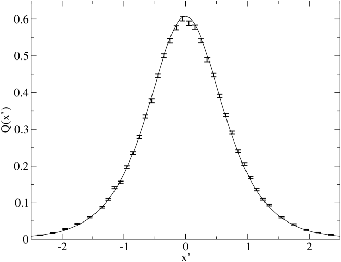
Figure 3: Reduced distribution of the Ising interface end point ($x^{\prime}=x/L$). The plain curve is the analytical result, data points are numerical results for $L=80$.

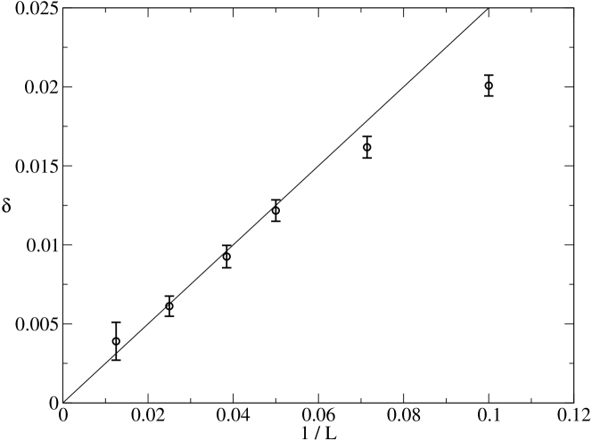
Figure 4: Value of the maximum absolute difference between the numerical and analytical integrated distributions of the Ising interface end point for $80\geq L\geq 10$. The straight line is just a guide to the eyes.

We thus get the distribution of end point position $x$. The distribution $Q(x^{\prime})$ of $x^{\prime}=x/L$ is to be compared to the theoretical one computed previously (14) (with $\kappa=3$) for a strip of width $\pi$. In the simulation variables, it reads:

$$Q(x^{\prime})=\frac{\pi}{I}\cosh(x^{\prime}\pi/2)^{-4/3}.$$ (15)

Where $I$ is in this case $6\;\Gamma(2/3)\;\Gamma(5/6)/\sqrt{\pi}\simeq 5.17422$. The theoretical and numerical distributions (for $L=80$) are shown on figure 3. They agree very well. To make a more precise statement, we considered the integrated distribution (for which the statistical error bars are much smaller) and computed the maximum $\delta$ of the absolute difference between the theoretical and numerical integrated distributions. The results are shown on figure 4. This difference converges nicely to zero at large $L$. Moreover the finite size corrections seems to be of order $1/L$. Note that the finite size corrections were expected to be at a least of order $1/L$ since the lattice spacing has a relative size of order $1/L$.

8 Conclusion.

Besides chordal and radial SLEs, dipolar SLEs are the only possible simple SLEs on simply connected planar domains which satisfy a left-right reflection symmetry. As illustrated in previous sections, they provide a generalization of chordal SLEs with more structures since the hulls do not totally fill the domain for $\kappa>4$. The fact that the bulk visiting probabilities we computed are harmonic functions is clearly related to the discrete harmonic explorer. The latter was defined in ref.[13] to provide a discrete analogue of chordal SLE at $\kappa=4$. It clearly can be generalized to yield a discrete analogue of dipolar SLE at $\kappa=4$ by dealing with harmonic functions with ’D;D;N’ boundary conditions to specify the probabilities of the excursion processes.

The harmonicity property of the visiting probabilities for $\kappa>4$ was unexpected from a CFT point of view. The origin of the non-harmonicity transition – ie. the fact the probabilities for a point to be on the left (or on the right) of the curve stop to be harmonic for $\kappa<4$ – is not clear to us. We however noticed that for $\kappa>4$ the probabilities for a point to be swallowed from the left (or from the right) are also not harmonic functions. These two breakdowns of harmonicity seem to be related by duality $\kappa\leftrightarrow 16/\kappa$.

Finally, numerical simulations of the Ising ferromagnet at criticality confirms the analytical results presented here as well as the CFT mapping.

Acknowledgements: Work supported in part by EC contract number HPRN-CT-2002-00325 of the EUCLID research training network.

Appendix A Appendix: analytical details on the function $F(z)$.

Here we gathered a few informations on the function

$$F(z)\equiv\int_{-\infty}^{z}\frac{du}{(\sinh u/2)^{4/\kappa}}.$$

We have to specify the analytical properties of $(\sinh z/2)^{-4/\kappa}$. It is such that ${\rm arg}(\sinh z/2)\in[0,\pi]$. Hence, $(\sinh z/2)^{-4/\kappa}$ is real on the positive real axis, equals to $e^{-i4\pi/\kappa}(\sinh|x|/2)^{-4/\kappa}$ on the negative real axis and equals to $e^{-i2\pi/\kappa}(\cosh x/2)^{-4/\kappa}$ on the upper boundary $z=i\pi+x$. One may verify that it is equivalent to $2^{4/\kappa}\,e^{-2z/\kappa}$ around $+\infty$, while it behaves as $2^{4/\kappa}\,e^{(2z-i4\pi)/\kappa}$ around $-\infty$ .

By analyticity, the contour of integration in the definition of $F(z)$ can be choose arbitrary inside the strip $\mathbb{S}_{1}$ but starting at $-\infty$. As a consequence, comparing the integration along the real axis $\mathbb{R}$ and along $i\pi+\mathbb{R}$ we learn that $F(0)=e^{-i4\pi/\kappa}\,J$ and that

$$F(+\infty)=e^{-i2\pi/\kappa}\ I=e^{-i4\pi/\kappa}\ J+J,$$

where $I=\int_{-\infty}^{+\infty}dy(\cosh y/2)^{-4/\kappa}$ and $J=\int_{0}^{+\infty}dy(\sinh y/2)^{-4/\kappa}$ as in the text. This leads to $I=2J\cos(2\pi/\kappa)$

For $z=a+ib$, $b\in[0,\pi]$, one may expand $\sinh z/2$ as

$$\sinh z/2=\sinh a/2\,\cos b/2+i\cosh a/2\sin b/2,$$

so that $(\sinh z/2)^{-4/\kappa}=R^{-4/\kappa}_{z}\,\exp(-i4\theta_{z}/\kappa)$ with

$$R_{z} = |\sinh z/2|,$$

$$\tan\theta_{z} = \coth a/2\,\tan b/2,\quad\theta_{z}\in[0,\pi].$$

The angle $\theta_{a+ib}$ decreases from $(\pi-b/2)$ to $b/2$ as $a$ varies from $-\infty$ to $+\infty$.

The functions $\Im{\rm m}[F(z)]$ and $\Im{\rm m}[e^{i2\pi/\kappa}\,F(z)]$ involved in eqs.(10,11), can be represented as:

$$\Im{\rm m}[F(z=x+ib)] = -\int_{-\infty}^{x}da\,R^{-4/\kappa}_{a+ib}\,\sin(4\theta_{a+ib}/\kappa),$$

$$\Im{\rm m}[e^{i2\pi/\kappa}\,F(z=x+ib)] = -\int_{-\infty}^{x}da\,R^{-4/\kappa}_{a+ib}\,\sin((4\theta_{a+ib}-2\pi)/\kappa).$$

Other representations can be written using different integration contours.

References

- [1] O. Schramm, Israel J. Math., 118, 221–288, (2000);
- [2] S. Rohde and O. Schramm, arXiv:math.PR/0106036; and references therein.
-
[3]
G. Lawler, O. Schramm and W. Werner,
(I):Acta Mathematica 187 (2001) 237–273; arXiv:math.PR/9911084
G. Lawler, O. Schramm and W. Werner, (II): Acta Mathematica 187 (2001) 275–308; arXiv:math.PR/0003156
G. Lawler, O. Schramm and W. Werner, (III): Ann. Henri Poincaré 38 (2002) 109–123. arXiv:math.PR/0005294. - [4] G. Lawler, introductory texts, including the draft of a book, may be found at http://www.math.cornell.edu/lawler
- [5] J. Cardy, J. Phys. A25 (1992) L201–206.
- [6] S. Smirnov, C.R. Acad. Sci. Paris 333 (2001) 239–244.
-
[7]
M. Bauer and D. Bernard,
Commun. Math. Phys. 239 (2003) 493–521, arXiv:hep-th/0210015, and
Phys. Lett. B543 (2002) 135–138;
M. Bauer and D. Bernard, Phys. Lett. B557 (2003) 309–316, arXiv-hep-th/0301064;
M. Bauer and D. Bernard, Ann. Henri Poincaré 5 (2004) 289–326, arXiv:math-ph/0305061. - [8] M. Bauer and D. Bernard, SLE, CFT and zig-zag probabilities, arXiv:math-ph/0401019.
- [9] J. Cardy, Nucl. Phys B324 (1989) 581.
- [10] B. Nienhuis, J. Stat. Phys. 34 (1983) 731.
- [11] Vl. Dotsenko and V. Fateev, Nucl. Phys. B240 (1984) 312–348 and Nucl. Phys. B251 (1985) 691–734;
- [12] Ph. Di Francesco, P. Mathieu and D. Senechal, Conformal field theory, Springer 1996.
- [13] O. Schramm, S. Sheffield, arXiv:math.PR/0310210.
- [14] J. Houdayer, Eur. Phys. Jour. B 22 (2001) 479–484.