Momentum Maps
and
Classical Fields
Part II: Canonical Analysis of Field Theories

II—CANONICAL ANALYSIS OF FIELD THEORIES

With the covariant formulation in hand from the first part of this book, we begin in this second part to study the canonical (or “instantaneous”) formulation of classical field theories. The canonical formluation works with fields defined as time-evolving cross sections of bundles over a Cauchy surface, rather than as sections of bundles over spacetime as in the covariant formulation. More precisely, for a given classical field theory, the (infinite-dimensional) instantaneous configuration space consists of the set $\mathcal{Y}_{\Sigma}$ of all smooth sections of a specified bundle $Y_{\Sigma}$ over a Cauchy surface $\Sigma$, and a solution to the field equations is represented by a trajectory in $\mathcal{Y}_{\Sigma}$. As in classical mechanics, the Lagrangian formulation of the field equations of a classical field theory is defined on the tangent bundle $T\mathcal{Y}_{\Sigma}$, and the Hamiltonian formulation is defined on the cotangent bundle $T^{*}\mathcal{Y}_{\Sigma}$, which has a canonically defined symplectic structure $\omega_{\Sigma}$.

To relate the canonical and the covariant approaches to classical field theory, we start in Chapter 5 by discussing embeddings $\Sigma\rightarrow X$ of Cauchy surfaces in spacetime, and considering the corresponding pull-back bundles $Y_{\Sigma}\rightarrow\Sigma$ of the covariant configuration bundle $Y\rightarrow X$. We go on in the same chapter to relate the covariant multisymplectic geometry of $(Z,\Omega)$ to the instantaneous symplectic geometry of $(T^{*}\mathcal{Y}_{\Sigma},\omega_{\Sigma})$ by showing that the multisymplectic form $\Omega$ on $Z$ naturally induces the symplectic form $\omega_{\Sigma}$ on $T^{*}\mathcal{Y}_{\Sigma}$.

The discussion in Chapter 5 concerns primarily kinematical structures, such as spaces of fields and their geometries, but does not involve the action principle or the field equations for a given classical field theory. In Chapter 6, we proceed to consider field dynamics. A crucial feature of our discussion here is the degeneracy of the Lagrangian functionals for the field theories of interest. As a consequence of this degeneracy, we have constraints on the choice of initial data, and gauge freedom in the evolution of the fields. Chapter 6 considers the role of initial value constraints and gauge transformations in field dynamics. The discussion is framed primarily in the Hamiltonian formulation of the dynamics.

One of the primary goals of this work is to show how momentum maps are used in classical field theories which have both initial value constraints and gauge freedom. In Chapter 7, we begin to do this by describing how the covariant momentum maps defined on the multiphase space $Z$ in Part I induce a generalization of momentum maps—“energy-momentum maps”—on the instantaneous phase spaces $T^{*}\mathcal{Y}_{\Sigma}$. We show that for a group action which leaves the Cauchy surface invariant, this energy-momentum map coincides with the usual notion of a momentum map. We also show, when the gauge group “includes” the spacetime diffeomorphism group, that one of the components of the energy-momentum map corresponding to spacetime diffeomorphisms can be identified (up to sign) with the Hamiltonian for the theory.

5 Symplectic Structures Associated with
Cauchy Surfaces

The transition from the covariant to the instantaneous formalism once a Cauchy surface (or a foliation by Cauchy surfaces) has been chosen is a central ingredient of this work. It will eventually be used to cast the field dynamics into adjoint form and to determine when the first class constraint set (in the sense of Dirac) is the zero set of an appropriate energy-momentum map.

5A Cauchy Surfaces and Spaces of Fields

In any particular field theory, we assume there is singled out a class of hypersurfaces which we call Cauchy surfaces. We will not give a precise definition here, but our usage of the term is intended to correspond to its meaning in general relativity (see, for instance, Hawking and Ellis [1973]).

Let $\Sigma$ be a compact (oriented, connected) boundaryless $n$-manifold. We denote by $\operatorname{Emb}(\Sigma,X)$ the space of all smooth embeddings of $\Sigma$ into $X$. (If the ($n+1$)-dimensional “spacetime” $X$ carries a nonvariational Lorentz metric, we then understand $\operatorname{Emb}(\Sigma,X)$ to be the space of smooth spacelike embeddings of $\Sigma$ into $X$.) As usual, many of the formal aspects of the constructions also work in the noncompact context with asymptotic conditions appropriate to the allowance of the necessary integrations by parts. However, the analysis necessary to cover the noncompact case need not be trivial; these considerations are important when dealing with isolated systems or asymptotically flat spacetimes. See Regge and Teitelboim [1974], Choquet–Bruhat, Fischer and Marsden [1979a], Śniatycki [1988], and Ashtekar, Bombelli, and Reula [1991].

For $\tau\in\operatorname{Emb}(\Sigma,X)$, let $\Sigma_{\tau}=\tau(\Sigma)$. The hypersurface $\Sigma_{\tau}$ will eventually be a Cauchy surface for the dynamics; we view $\Sigma$ as a reference or model Cauchy surface. We will not need to topologize $\operatorname{Emb}(\Sigma,X)$ in this paper; however, we note that when completed in appropriate $C^{k}$ or Sobolev topologies, $\operatorname{Emb}(\Sigma,X)$ and other manifolds of maps introduced below are known to be smooth manifolds (see, for example, Palais [1968] and Ebin and Marsden [1970]).

If $\pi_{X\mspace{-1.5mu}K}:K\to X$ is a fiber bundle over $X$, then the space of smooth sections of the bundle will be denoted by the corresponding script letter, in this case $\mathcal{K}$. Occasionally, when this notation might be confusing, we will resort to the notation $\Gamma(K)$ or $\Gamma(X,K)$. We let $K_{\tau}$ denote the restriction of the bundle $K$ to $\Sigma_{\tau}\subset X$ and let the corresponding script letter denote the space of its smooth sections, in this case $\mathcal{K}_{\tau}$. The collection of all $\mathcal{K}_{\tau}$ as $\tau$ ranges over $\operatorname{Emb}(\Sigma,X)$ forms a bundle over $\operatorname{Emb}(\Sigma,X)$ which we will denote $\mathcal{K}^{\Sigma}$.

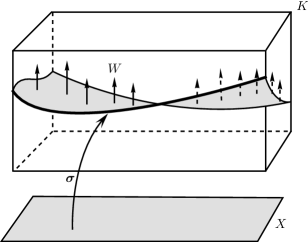
Figure 5.1: A tangent vector $W\in T_{\sigma}\mathcal{K}$

The tangent space to $\mathcal{K}$ at a point $\sigma$ is given by

$$T_{\sigma}\mathcal{K}=\left\{W:X\to V\mspace{-1.5mu}K\bigm{|}W\text{ covers }\sigma\right\},$$ (5A.1)

where $V\mspace{-1.5mu}K$ denotes the vertical tangent bundle of $K$. See Figure 5-1.

Similarly, the smooth cotangent space to $\mathcal{K}$ at $\sigma$ is

$$T^{*}_{\sigma}\mathcal{K}=\left\{\pi:X\to L(V\mspace{-1.5mu}K,\Lambda^{n+1}X)\bigm{|}\pi\text{ covers }\sigma\right\},$$ (5A.2)

where $L(V\mspace{-1.5mu}K,\Lambda^{n+1}X)$ is the vector bundle over $K$ whose fiber at $k\in K_{x}$ is the set of linear maps from $V_{k}K$ to $\Lambda^{n+1}_{x}X$. The natural pairing of $T^{*}_{\sigma}\mathcal{K}$ with $T_{\sigma}\mathcal{K}$ is given by integration:

$$\langle\pi,V\rangle=\int_{X}\pi(V).$$ (5A.3)

One obtains similar formulas for $\mathcal{K}_{\tau}$ from the above by replacing $X$ with $\Sigma_{\tau}$ and $K$ with $K_{\tau}$ throughout (and replacing $n+1$ by $n$ in (5A.2)). See Figure 5-2.

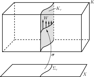
Figure 5.2: A tangent vector $W\in T_{\sigma}\mathcal{K}_{\tau}$

If $\xi_{K}$ is any $\pi_{X\mspace{-1.5mu}K}$-projectable vector field on $K$, we define the Lie derivative of $\sigma\in\mathcal{K}$ along $\xi_{K}$ to be the element of $T_{\sigma}\mathcal{K}$ given by

$$\pounds_{\xi_{K}}\sigma=T\sigma\circ\xi_{X}-\xi_{K}\circ\sigma.$$ (5A.4)

Note that $-\pounds_{\xi_{K}}\sigma$ is exactly the vertical component of $\xi_{K}\circ\sigma$. In coordinates $(x^{\mu},k^{A})$ on $K$ we have

$$(\pounds_{\xi_{K}}\sigma)^{A}=\sigma^{A}{}_{,\mu}\xi^{\mu}-\xi^{A}\circ\sigma,$$ (5A.5)

where $\xi_{K}=(\xi^{\mu},\xi^{A}).$

Finally, if $f$ is a map $\mathcal{K}\rightarrow\mathcal{F}(X)$ we define the “formal” partial derivatives $D_{\mu}f:\mathcal{K}\rightarrow\mathcal{F}(X)$ via

$$D_{\mu}f(\sigma)=f(\sigma)_{,\mu}.$$ (5A.6)

Intrinsically, this is the coordinate representation of the differential of the real valued function $f(\sigma)$.

5B Canonical Forms on $T^{*}\mathcal{Y}_{\tau}$

In the instantaneous formalism the configuration space at “time” $\tau\in\operatorname{Emb}(\Sigma,X)$ will be denoted $\mathcal{Y}_{\tau}$, hereafter called the $\tau$-configuration space. Likewise, the $\tau$-phase space is$T^{*}\mathcal{Y}_{\tau}$, the smooth cotangent bundle of $\mathcal{Y}_{\tau}$ with its canonical one-form $\theta_{\tau}$ and canonical two-form $\omega_{\tau}$. These forms are defined using the same construction as for ordinary cotangent bundles (see Abraham and Marsden [1978] or Chernoff and Marsden [1974]). Specifically, we define $\theta_{\tau}$ by

$$\theta_{\tau}(\varphi,\pi)(V)=\int_{\Sigma_{\tau}}\pi(T\pi_{\mathcal{Y}_{\tau},T^{*}\mathcal{Y}_{\tau}}\cdot V)$$ (5B.1)

where $(\varphi,\pi)$ denotes a point in $T^{*}\mathcal{Y}_{\tau}$, $V\in T_{(\varphi,\pi)}T^{*}\mathcal{Y}_{\tau}$ and $\pi_{\mathcal{Y}_{\tau},T^{*}\mathcal{Y}_{\tau}}:T^{*}\mathcal{Y}_{\tau}\to\mathcal{Y}_{\tau}$ is the cotangent bundle projection. We define

$$\omega_{\tau}=-\mathbf{d}\theta_{\tau}.$$ (5B.2)

We now develop coordinate expressions for these forms. To this end choose a chart$\left(x^{0},x^{1},\dots,x^{n}\right)$ on $X$ which is adapted to $\tau$ in the sense that $\Sigma_{\tau}$ is locally a level set of $x^{0}$. Then an element $\pi\in T^{*}_{\varphi}\mathcal{Y}_{\tau}$, regarded as a map $\pi~{}:~{}\Sigma_{\tau}~{}\to~{}L(VY_{\tau},\Lambda^{n}\Sigma_{\tau})$, is expressible as

$$\pi=\pi_{A}\,dy^{A}\otimes d^{\mspace{1.5mu}n}\mspace{-1.5mu}x_{0},$$ (5B.3)

so for the canonical one- and two-forms on $T^{*}\mathcal{Y}_{\tau}$ we get

$$\theta_{\tau}(\varphi,\pi)=\int_{\Sigma_{\tau}}\pi_{A}\,d\varphi^{A}\otimes d^{\mspace{1.5mu}n}\mspace{-1.5mu}x_{0}$$ (5B.4)

and

$$\omega_{\tau}(\varphi,\pi)=\int_{\Sigma_{\tau}}(d\varphi^{A}\wedge d\pi_{A})\otimes d^{\mspace{1.5mu}n}\mspace{-1.5mu}x_{0}.$$ (5B.5)

For example, if $V\in T_{(\varphi,\pi)}(T^{*}\mathcal{Y}_{\tau})$ is given in adapted coordinates by $V=(V^{A},W_{A})$, then we have

$$\theta_{\tau}(\varphi,\pi)(V)=\int_{\Sigma_{\tau}}\pi_{A}V^{A}d^{\mspace{1.5mu}n}\mspace{-1.5mu}x_{0}.$$

5C Presymplectic Structure on $\mathcal{Z}_{\tau}$

To relate the symplectic manifold $T^{*}\mathcal{Y}_{\tau}$ to the multisymplectic manifold $Z$, we first use the multisymplectic structure on $Z$ to induce a presymplectic structure on $\mathcal{Z}_{\tau}$ and then identify $T^{*}\mathcal{Y}_{\tau}$ with the quotient of $\mathcal{Z}_{\tau}$ by the kernel of this presymplectic form. Specifically, define the canonical one-form $\Theta_{\tau}$ on $\mathcal{Z}_{\tau}$ by

$$\Theta_{\tau}(\sigma)(V)=\int_{\Sigma_{\tau}}\sigma^{*}(\mathbf{i}_{V}\Theta),$$ (5C.1)

where $\sigma\in\mathcal{Z}_{\tau}$, $V\in T_{\sigma}\mathcal{Z}_{\tau}$, and $\Theta$ is the canonical $(n+1)$-form on $Z$ given by (2B.9). The canonical two-form $\Omega_{\tau}$ on $\mathcal{Z}_{\tau}$ is

$$\Omega_{\tau}=-\mathbf{d}\Theta_{\tau}.$$ (5C.2)

Lemma 5.1.

At $\sigma\in\mathcal{Z}_{\tau}$ and with $\Omega$ given by (2B.10), we have

$$\Omega_{\tau}(\sigma)(V,W)=\int_{\Sigma_{\tau}}\sigma^{*}(\mathbf{i}_{W}\mathbf{i}_{V}\Omega).$$ (5C.3)

• Extend $V,W$ to vector fields $\mathcal{V},\mathcal{W}$ on $\mathcal{Z}_{\tau}$ by fixing $\pi_{X\mspace{-1.5mu}Z}$-vertical vector fields $v,w$ on $Z_{\tau}$ such that $V=v\circ\sigma$ and $W=w\circ\sigma$ and letting $\mathcal{V}(\rho)=v\circ\rho$ and $\mathcal{W}(\rho)=w\circ\rho$ for $\rho\in\mathcal{Z}_{\tau}$. Note that if $f_{\lambda}$ is the flow of $w$, $\mathcal{F}_{\lambda}(\rho)=f_{\lambda}\circ\rho$ is the flow of $\mathcal{W}$. Then, from the definition of the bracket in terms of flows, one finds that

  $$[\mathcal{V},\mathcal{W}](\rho)=[v,w]\circ\rho.$$

  The derivative of $\Theta_{\tau}(\mathcal{V})$ along $\mathcal{W}$ at $\sigma$ is

  $$\mathcal{W}\left[\Theta_{\tau}(\mathcal{V})\right](\sigma) =\left.\frac{d}{d\lambda}\left[\Theta_{\tau}(\mathcal{V})\circ\mathcal{F}_{\lambda}(\sigma)\right]\right|_{\lambda=0}=\left.\frac{d}{d\lambda}\left[\int_{\Sigma_{\tau}}\mathcal{F}_{\lambda}(\sigma)^{*}(\mathbf{i}_{v}\Theta)\right]\right|_{\lambda=0}$$

  $$=\left.\frac{d}{d\lambda}\left[\int_{\Sigma_{\tau}}\sigma^{*}f^{*}_{\lambda}(\mathbf{i}_{v}\Theta)\right]\right|_{\lambda=0}=\int_{\Sigma_{\tau}}\sigma^{*}[\pounds_{w}\mathbf{i}_{v}\Theta].$$

  Thus, at $\sigma\in\mathcal{Z}_{\tau}$,

  $$\mathbf{d}\Theta_{\tau}(\mathcal{V},\mathcal{W}) =\mathcal{V}\left[\Theta_{\tau}(\mathcal{W})]-\mathcal{W}[\Theta_{\tau}(\mathcal{V})]-\Theta_{\tau}([\mathcal{V},\mathcal{W}\right])$$

  $$=\int_{\Sigma_{\tau}}\sigma^{*}\left[\pounds_{v}\mathbf{i}_{w}\Theta-\pounds_{w}\mathbf{i}_{v}\Theta-\mathbf{i}_{[v,w]}\Theta\right]$$

  $$=\int_{\Sigma_{\tau}}\sigma^{*}(-\mathbf{d}\mathbf{i}_{w}\mathbf{i}_{v}\Theta+\mathbf{i}_{w}\mathbf{i}_{v}\mathbf{d}\Theta),$$

  and the first term vanishes by the definitions of $Z$ and $\Theta$, as both $v,w$ are $\pi_{X\mspace{-1.5mu}Z}$-vertical. ∎

The two-form $\Omega_{\tau}$ on $\mathcal{Z}_{\tau}$ is closed, but it has a nontrivial kernel, as the following development will show.

5D Reduction of $\mathcal{Z}_{\tau}$ to $T^{*}\mathcal{Y}_{\tau}$

Our next goal is to prove that $\mathcal{Z}_{\tau}/\ker\Omega_{\tau}$ is canonically isomorphic to $T^{*}\mathcal{Y}_{\tau}$ and that the inherited symplectic form on the former is isomorphic to the canonical one on the latter. To do this, define a vector bundle map $R_{\tau}:\mathcal{Z}_{\tau}\to T^{*}\mathcal{Y}_{\tau}$ over $\mathcal{Y}_{\tau}$ by

$$\left\langle R_{\tau}(\sigma),V\right\rangle=\int_{\Sigma_{\tau}}\varphi^{*}(\mathbf{i}_{V}\sigma),$$ (5D.1)

where $\varphi=\pi_{Y\!Z}\circ\sigma$ and $V\in T_{\varphi}\mathcal{Y}_{\tau}$; the integrand in (5D.1) at a point $x\in\Sigma_{\tau}$ is the interior product of $V(x)$ with $\sigma(x)$, resulting in an $n$-form on $Y$, which is then pulled back along $\varphi$ to an $n$-form on $\Sigma_{\tau}$ at $x$. Interpreted as a map of $\Sigma_{\tau}$ to $L(VY_{\tau},\Lambda^{n}\Sigma_{\tau})$ which covers $\varphi$, $R_{\tau}(\sigma)$ is given by

$$\left\langle R_{\tau}(\sigma)(x),v\right\rangle=\varphi^{*}\mathbf{i}_{v}\sigma(x),$$ (5D.2)

where $v\in V_{\varphi(x)}Y_{\tau}$. In adapted coordinates, $\sigma\in\mathcal{Z}_{\tau}$ takes the form

$$(p_{A}{}^{\mu}\circ\sigma)\,dy^{A}\wedge d^{\mspace{1.5mu}n}\mspace{-1.5mu}x_{\mu}+(p\circ\sigma)\,d^{\mspace{1.5mu}n+1}\mspace{-1.5mu}x,$$ (5D.3)

and so we may write

$$R_{\tau}(\sigma)=(p_{A}{}^{0}\circ\sigma)\,dy^{A}\otimes d^{\mspace{1.5mu}n}\mspace{-1.5mu}x_{0}.$$ (5D.4)

Comparing (5D.4) with (5B.3), we see that the instantaneous momenta $\pi_{A}$ correspond to the temporal components of the multimomenta $p_{A}{}^{\mu}$. Moreover, $R_{\tau}$ is obviously a surjective submersion with

$$\ker R_{\tau}=\left\{\sigma\in\mathcal{Z}_{\tau}\mid p_{A}{}^{0}\circ\sigma=0\right\}.$$

• Although we have defined $R_{\tau}$ as a map on sections from $\mathcal{Z}_{\tau}$ to $T^{*}\mathcal{Y}_{\tau}$, in actuality $R_{\tau}$ is a pointwise operation. We may in fact write (5D.2) as $R_{\tau}(\sigma)=r_{\tau}\circ\sigma$, where

  $$r_{\tau}:Z_{\tau}\to V^{*}Y_{\tau}\otimes\Lambda^{n}\Sigma_{\tau}$$

  is a bundle map over $Y_{\tau}$. From (5D.3) and (5D.4), we see that in coordinate form $r_{\tau}(p,p_{A}{}^{\mu})=p_{A}{}^{0}$ with

  $$\ker r_{\tau}=\left\{p_{A}{}^{i}dy^{A}\otimes d^{\mspace{1.5mu}n}\mspace{-1.5mu}x_{i}+p\,d^{\mspace{1.5mu}n+1}\mspace{-1.5mu}x\in Z_{\tau}\right\}. \blacklozenge$$

   

Proposition 5.2.

We have

$$R^{*}_{\tau}\theta_{\tau}=\Theta_{\tau}.$$ (5D.5)

• Let $V\in T_{\sigma}\mathcal{Z}_{\tau}$. By the definitions of pull-back and the canonical one-form,

  $$\left\langle(R^{*}_{\tau}\theta_{\tau})(\sigma),V\right\rangle=\left\langle\theta_{\tau}(R_{\tau}(\sigma)),TR_{\tau}\cdot V\right\rangle=\langle R_{\tau}(\sigma),T\pi_{\mathcal{Y}_{\tau},T^{*}\mathcal{Y}_{\tau}}\cdot TR_{\tau}\cdot V\rangle.$$

  However, since $R_{\tau}$ covers the identity,

  $$\pi_{\mathcal{Y}_{\tau},T^{*}\mathcal{Y}_{\tau}}\circ R_{\tau}=\pi_{\mathcal{Y}_{\tau},\mathcal{Z}_{\tau}}$$

  and so

  $$T\pi_{\mathcal{Y}_{\tau},T^{*}\mathcal{Y}_{\tau}}\cdot TR_{\tau}\cdot V=T\pi_{\mathcal{Y}_{\tau},\mathcal{Z}_{\tau}}\cdot V=T\pi_{Y\!Z}\circ V.$$

  Thus by (5D.1), with $\varphi=\pi_{Y\!Z}\circ\sigma$,

  $$\left\langle R^{*}_{\tau}\theta_{\tau}(\sigma),V\right\rangle =\langle R_{\tau}(\sigma),T\pi_{Y\!Z}\circ V\rangle=\int_{\Sigma_{\tau}}\varphi^{*}((T\pi_{Y\!Z}\circ V)\mathbin{\hbox to6.0pt{\vrule height=0.4pt,width=5.0pt,depth=0.0pt\kern-0.4pt\vrule height=6.0pt,width=0.4pt,depth=0.0pt\hss}}\sigma)$$

  $$=\int_{\Sigma_{\tau}}\sigma^{*}\pi^{*}_{Y\!Z}((T\pi_{Y\!Z}\circ V)\mathbin{\hbox to6.0pt{\vrule height=0.4pt,width=5.0pt,depth=0.0pt\kern-0.4pt\vrule height=6.0pt,width=0.4pt,depth=0.0pt\hss}}\sigma)$$

  $$=\int_{\Sigma_{\tau}}\sigma^{*}(V\mathbin{\hbox to6.0pt{\vrule height=0.4pt,width=5.0pt,depth=0.0pt\kern-0.4pt\vrule height=6.0pt,width=0.4pt,depth=0.0pt\hss}}\,\pi^{*}_{Y\!Z}\sigma).$$

  However, by (2B.7) and (2B.9), $\pi^{*}_{Y\!Z}\sigma=\Theta\circ\sigma$. Thus by (5C.1),

  $$\left\langle R^{*}_{\tau}\theta_{\tau}(\sigma),V\right\rangle=\left\langle\Theta_{\tau}(\sigma),V\right\rangle.$$ ∎

  ∎

Corollary 5.3.

1. $R^{*}_{\tau}\omega_{\tau}=\Omega_{\tau}$.

2. $\ker T_{\sigma}R_{\tau}=\ker\Omega_{\tau}(\sigma)$.

3. The induced quotient map $\mathcal{Z}_{\tau}/\ker R_{\tau}=\mathcal{Z}_{\tau}/\ker\Omega_{\tau}\to T^{*}\mathcal{Y}_{\tau}$ is a symplectic diffeomorphism.

• (i) follows by taking the exterior derivative of (5D.5). (ii) follows from (i), the (weak) nondegeneracy of $\omega_{\tau}$, the definition of pull-back and the fact that $R_{\tau}$ is a submersion. Finally, (iii) follows from (i), (ii), and the fact that $R_{\tau}$ is a surjective vector bundle map between vector bundles over $\mathcal{Y}_{\tau}$. ∎

Thus, for each Cauchy surface $\Sigma_{\tau}$, the multisymplectic structure $\Omega$ on $Z$ induces a presymplectic structure $\Omega_{\tau}$ on $\mathcal{Z}_{\tau}$, and this in turn induces the canonical symplectic structure $\omega_{\tau}$ on the instantaneous phase space $T^{*}\mathcal{Y}_{\tau}$. Alternative constructions of $\Theta_{\tau}$ and $\omega_{\tau}$ are given in Zuckerman [1986], Crnković and Witten [1987], and Ashtekar, Bombelli, and Reula [1991].

 

a   Particle Mechanics.

For particle mechanics $\Sigma$ is a point, and $\tau$ maps $\Sigma$ to some $t\in\mathbb{R}$. We identify $\mathcal{Y}_{\tau}$ with $Q$ and $\mathcal{Z}_{\tau}$ with $\mathbb{R}\times T^{*}Q$, with coordinates $(q^{A},p,p_{A})$. The one-form $\theta_{\tau}$ is $\theta_{\tau}=p_{A}dq^{A}$ and $R_{\tau}$ is given by $(q^{A},p,p_{A})\mapsto(q^{A},p_{A})$. Thus the $\tau$-phase space is just $T^{*}Q$, and the process of reducing the multisymplectic formalism to the instantaneous formalism in particle mechanics is simply reduction to the autonomous case.

b   Electromagnetism.

In the case of electromagnetism, $\Sigma$ is a 3-manifold and $\tau\in\operatorname{Emb}(\Sigma,X)$ is a parametrized spacelike hypersurface. The space $\mathcal{Y}_{\tau}$ consists of fields $A_{\nu}$ over $\Sigma_{\tau}$, $T^{*}\mathcal{Y}_{\tau}$ consists of fields and their conjugate momenta $(A_{\nu},\mathfrak{E}^{\nu})$ on $\Sigma_{\tau}$, while the space $\mathcal{Z}_{\tau}$ consists of fields and multimomenta fields $(A_{\nu},p,\mathfrak{F}^{\nu\mu})$ on $\Sigma_{\tau}$. In adapted coordinates the map $R_{\tau}$ is given by

$$(A_{\nu},p,\mathfrak{F}^{\nu\mu})\mapsto(A_{\nu},\mathfrak{E}^{\nu}),$$ (5D.6)

where $\mathfrak{E}^{\nu}=\mathfrak{F}^{\nu 0}$. The canonical momentum $\mathfrak{E}^{\nu}$ can thus be identified with the negative of the electric field density. The symplectic structure on $T^{*}\mathcal{Y}_{\tau}$ takes the form

$$\omega_{\tau}(A,\mathfrak{E})=\int_{\Sigma_{\tau}}(dA_{\nu}\wedge d\mathfrak{E}^{\nu})\otimes d^{\mspace{1.5mu}3}\mspace{-1.5mu}x_{0}.$$ (5D.7)

When electromagnetism is parametrized, we simply append the metric $g$ to to the other field variables as a parameter. Let $S_{2}^{\mspace{1.5mu}3,1}(X,\Sigma_{\tau})$ denote the subbundle of $S_{2}^{\mspace{1.5mu}3,1}(X)$ consisting of Lorentz metrics relative to which $\Sigma_{\tau}$ is spacelike. Thus we replace $\mathcal{Y}_{\tau}$ by

$$\tilde{\mathcal{Y}}_{\tau}=\mathcal{Y}_{\tau}\times\mathcal{S}_{2}^{3,1}(X,\Sigma_{\tau})_{\tau},$$

which consists of sections $(A;g)$ of $\tilde{Y}=Y\times S_{2}^{\mspace{1.5mu}3,1}(X,\Sigma_{\tau})$ over $\Sigma_{\tau}$. Similarly, we replace $\mathcal{Z}_{\tau}$ by

$$\mathcal{Z}_{\tau}\times\mathcal{S}_{2}^{3,1}(X,\Sigma_{\tau})_{\tau},\$$

etc. The metric just gets carried along by $R_{\tau}$ in (5D.6), and the expression (5D.7) for $\omega_{\tau}$ remains unaltered.

c   A Topological Field Theory.

Since in a topological field theory there is no metric on $X$, it does not make sense to speak of “spacelike hypersurfaces” (although we shall continue to informally refer to $\Sigma_{\tau}$ as a “Cauchy surface”). Thus we may take $\tau$ to be any embedding of $\Sigma$ into $X$.

Other than this, along with the fact that $\Sigma$ is 2-dimensional, Chern–Simons theory is much the same as electromagnetism. Specifically, ${\mathcal{Y}}_{\tau}$ consists of fields $A_{\nu}$ over $\Sigma_{\tau}$, $T^{*}{\mathcal{Y}}_{\tau}$ consists of fields and their conjugate momenta $(A_{\nu},\pi^{\nu})$ over $\Sigma_{\tau}$, and ${\mathcal{Z}}_{\tau}$ consists of fields and their multimomenta $(A_{\nu},p,p^{\nu\mu})$ over $\Sigma_{\tau}$. Then $R_{\tau}$ and $\omega_{\tau}$ are given by

$$(A_{\nu},p,p^{\nu\mu})\mapsto(A_{\nu},\pi^{\nu})$$ (5D.8)

and

$$\omega_{\tau}(A_{\nu},\pi^{\nu})=\int_{\Sigma_{\tau}}(dA_{\nu}\wedge d\pi^{\nu})\otimes d^{\mspace{1.5mu}2}\mspace{-1.5mu}x_{0}$$ (5D.9)

respectively, where $\pi^{\nu}=p^{\nu 0}$.

d   Bosonic Strings.

Here $\Sigma$ is a 1-manifold and $\tau\in\operatorname{Emb}(\Sigma,X)$ is a parametrized curve in $X$. Since $Y=(X\times M)\times_{X}S^{1,1}_{2}(X)$, $\mathcal{Y}_{\tau}$ consists of fields $(\varphi^{A},h_{\sigma\mspace{-1.5mu}\rho})$ over $\Sigma_{\tau}$, $T^{*}\mathcal{Y}_{\tau}$ consists of fields and their conjugate momenta $(\varphi^{A},h_{\sigma\mspace{-1.5mu}\rho},\pi_{A},\rho^{\sigma\mspace{-1.5mu}\rho})$, and $\mathcal{Z}_{\tau}$ consists of fields and their multimomenta $(\varphi^{A},h_{\sigma\mspace{-1.5mu}\rho},p,p_{A}{}^{\mu},q^{\sigma\mspace{-1.5mu}\rho\mu})$. In adapted coordinates, the map $R_{\tau}$ is

$$(\varphi^{A},h_{\sigma\mspace{-1.5mu}\rho},p,p_{A}{}^{\mu},q^{\sigma\mspace{-1.5mu}\rho\mu})\mapsto(\varphi^{A},h_{\sigma\mspace{-1.5mu}\rho},\pi_{A},\rho^{\sigma\mspace{-1.5mu}\rho})$$ (5D.10)

where $\pi_{A}=p_{A}{}^{0}$ and $\rho^{\sigma\mspace{-1.5mu}\rho}=q^{\sigma\mspace{-1.5mu}\rho\mspace{1.5mu}0}$. The symplectic form on $T^{*}\mathcal{Y}_{\tau}$ is then

$$\quad\qquad\omega_{\tau}(\varphi,h,\pi,\rho)=\int_{\Sigma_{\tau}}(d\varphi^{A}\wedge d\pi_{A}+dh_{\sigma\mspace{-1.5mu}\rho}\wedge d\rho^{\sigma\mspace{-1.5mu}\rho})\otimes d^{\mspace{1.5mu}1}\mspace{-1.5mu}x_{0}.\qquad\blacklozenge$$ (5D.11)

 

6 Initial Value Analysis of Field Theories

In the previous chapter we showed how to space + time decompose multisymplectic structures. Here we perform a similar decomposition of dynamics using the notion of slicings. This material puts the standard initial value analysis into our context, with a few clarifications concerning how to intrinsically split off the time derivatives of fields in the passage from the covariant to the instantaneous pictures. A main result of this chapter is that the dynamics is compatible with the space + time decomposition in the sense that Hamiltonian dynamics in the instantaneous formalism corresponds directly to the covariant Lagrangian dynamics of Chapter 3; see §6D. We also discuss a symplectic version of the Dirac–Bergmann treatment of degenerate Hamiltonian systems, initial value constraints, and gauge transformations in §6E.

6A Slicings

To discuss dynamics, that is, how fields evolve in time, we define a global notion of “time.” This is accomplished by introducing “slicings” of spacetime and the relevant bundles over it.

A slicing of an $(n+1)$-dimensional spacetime $X$ consists of an $n$-dimensional manifold $\Sigma$ (sometimes known as a reference Cauchy surface) and a diffeomorphism

$$\mathfrak{s}_{X}:\Sigma\times\mathbb{R}\to X.$$

For $\lambda\in\mathbb{R}$, we write $\Sigma_{\lambda}=\mathfrak{s}_{X}(\Sigma\times\{\lambda\})$ and $\tau_{\lambda}:\Sigma\to\Sigma_{\lambda}\subset X$ for the embedding defined by $\tau_{\lambda}(x)=\mathfrak{s}_{X}(x,\lambda)$. See Figure 6-1. The slicing parameter $\lambda$ gives rise to a global notion of “time” on $X$ which need not coincide with locally defined coordinate time, nor with proper time along the curves $\lambda\mapsto\mathfrak{s}_{X}(x,\lambda)$. The generator of $\mathfrak{s}_{X}$ is the vector field $\zeta_{X}$ on $X$ defined by

$$\frac{\partial}{\partial\lambda}\mathfrak{s}_{X}(x,\lambda)=\zeta_{X}(\mathfrak{s}_{X}(x,\lambda)).$$

Alternatively, $\zeta_{X}$ is the push-forward by $\mathfrak{s}_{X}$ of the standard vector field ${\partial}/{\partial\lambda}$ on $\Sigma\times\mathbb{R}$; that is,

$$\zeta_{X}=T\mathfrak{s}_{X}\cdot\frac{\partial}{\partial\lambda}.$$ (6A.1)

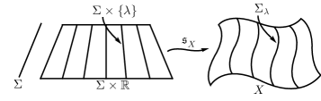
Figure 6.1: A slicing of spacetime

Given a bundle $K\to X$ and a slicing $\mathfrak{s}_{X}$ of $X$, a compatible slicing of $K$ is a bundle $K_{\Sigma}\to\Sigma$ and a bundle diffeomorphism $\mathfrak{s}_{K}:K_{\Sigma}\times\mathbb{R}\to K$ such that the diagram

$$\begin{CD}K_{\Sigma}\times\mathbb{R}@>{\mathfrak{s}_{K}}>{}>K\\ @V{}V{}V@V{}V{}V\\ \Sigma\times\mathbb{R}@>{\mathfrak{s}_{X}}>{}>X\end{CD}$$ (6A.2)

commutes, where the vertical arrows are bundle projections. We write $K_{\lambda}=\mathfrak{s}_{K}(K_{\Sigma}\times\{\lambda\})$ and $\mathfrak{s}_{\lambda}:K_{\Sigma}\to K_{\lambda}\subset K$ for the embedding defined by $\mathfrak{s}_{\lambda}(k)=\mathfrak{s}_{K}(k,\lambda)$, as in Figure 6-2. The generating vector field $\zeta_{K}$ of $\mathfrak{s}_{K}$ is defined by a formula analogous to (6A.1). Note that $\zeta_{K}$ and $\zeta_{X}$ are complete and everywhere transverse to the slices $K_{\lambda}$ and $\Sigma_{\lambda}$, respectively.

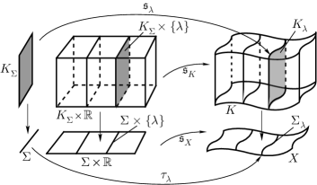
Figure 6.2: A slicing of the bundle $K$

Every compatible slicing $(\mathfrak{s}_{K},\mathfrak{s}_{X})$ of $K\to X$ defines a one-parameter group of bundle automorphisms: the flow $f_{\lambda}$ of the generating vector field $\zeta_{K}$, which is given by

$$f_{\lambda}(k)=\mathfrak{s}_{K}(\mathfrak{s}_{K}^{-1}(k)+\lambda),$$

where “$+\;\lambda$” means addition of $\lambda$ to the second factor of $K_{\Sigma}\times\mathbb{R}$. This flow is fiber-preserving since $\zeta_{K}$ projects to $\zeta_{X}$. Conversely, let $f_{\lambda}$ be a fiber-preserving flow on $K$ with generating vector field $\zeta_{K}$. Then $\zeta_{K}$ along with a choice of Cauchy surface $\Sigma_{\tau}$ such that $\zeta_{X}\pitchfork\Sigma_{\tau}$ determines (at least in a neighborhood of $K_{\tau}$ in $K$) a slicing $\mathfrak{s}_{K}:K_{\tau}\times\mathbb{R}\to K$ according to $\mathfrak{s}_{K}(k,\lambda)=f_{\lambda}(k)$. Any other slicing corresponding to the above data differs from this $\mathfrak{s}_{K}$ by a diffeomorphism.

Slicings of bundles give rise to trivializations of associated spaces of sections. Given $K\to X$, recall from §5A that we have the bundle

$$\mathcal{K}^{\Sigma}=\bigcup_{\tau\in\operatorname{Emb}(\Sigma,X)}\mathcal{K}_{\tau}$$

over $\operatorname{Emb}(\Sigma,X)$, where $\mathcal{K}_{\tau}$ is the space of sections of $K_{\tau}=K\mspace{-1.5mu}\!\bigm{|}\!\Sigma_{\tau}$. Let $\mathcal{K}^{\tau}$ denote the portion of $\mathcal{K}^{\Sigma}$ that lies over the curve of embeddings $\lambda\mapsto\tau_{\lambda}$, where $\lambda\in\mathbb{R}$. In other words,

$$\mathcal{K}^{\tau}=\bigcup_{\lambda\in\mathbb{R}}\mathcal{K}_{\lambda}.$$

The slicing $\mathfrak{s}_{K}:K_{\Sigma}\times\mathbb{R}\to K$ induces a trivialization $\mathfrak{s}_{\mathcal{K}}:\mathcal{K}_{\Sigma}\times\mathbb{R}\to\mathcal{K}^{\tau}$ defined by

$$\mathfrak{s}_{\mathcal{K}}(\sigma_{\Sigma},\lambda)=\mathfrak{s}_{\lambda}\circ\sigma_{\Sigma}\circ\tau_{\lambda}^{-1}.$$ (6A.3)

Let $\zeta_{\mathcal{K}}$ be the pushforward of ${\partial}/{\partial\lambda}$ by means of this trivialization; then from (6A.3),

$$\zeta_{\mathcal{K}}(\sigma)=\zeta_{K}\circ\sigma.$$ (6A.4)

See Figure 6-3.

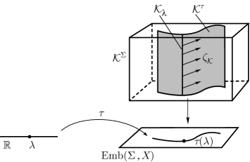
Figure 6.3: Bundles of spaces of sections

• A slicing $\mathfrak{s}_{X}$ of $X$ gives rise to at least one compatible slicing $\mathfrak{s}_{K}$ of any bundle $K\to X$, since $X\approx\Sigma\times\mathbb{R}$ is then homotopic to $\Sigma$.

2.

In many examples, $Y$ is a tensor bundle over $X$, so $\mathfrak{s}_{Y}$ can naturally be induced by a slicing $\mathfrak{s}_{X}$ of $X$. Similarly, in Yang–Mills theory, slicings of the connection bundle are naturally induced by slicings of the theory’s principal bundle.

3.

Slicings of the configuration bundle $Y\to X$ naturally induce slicings of certain bundles over it. For example, a slicing $\mathfrak{s}_{Y}$ of $Y$ induces a slicing $\mathfrak{s}_{Z}$ of $Z$ by push-forward; if $\zeta_{Y}$ generates $\mathfrak{s}_{Y}$, then $\mathfrak{s}_{Z}$ is generated by the canonical lift $\zeta_{Z}$ of $\zeta_{Y}$ to $Z$. (As a consequence, $\pounds_{\zeta_{Z}}\Theta=0$.) Likewise, a slicing of $J^{1}Y$ is generated by the jet prolongation $\zeta_{J^{1}Y}=j^{1}\zeta_{Y}$ of $\zeta_{Y}$ to $J^{1}Y$.

4.

When considering certain field theories, one may wish to modify these constructions slightly. In gravity, for example, one considers only those pairs of metrics and slicings for which each $\Sigma_{\lambda}$ is spacelike. This is an open and invariant condition and so the nature of the construction is not materially changed.

5.

It may happen that $X$ is sufficiently complicated topologically that it cannot be globally split as $\Sigma\times\mathbb{R}$ for any $\Sigma$. In such cases one can only slice portions of spacetime and our constructions must be understood in a restricted sense. However, for globally hyperbolic spacetimes, a well-known result of Geroch (see Hawking and Ellis [1973]) states that $X$ is indeed diffeomorphic to $\Sigma\times\mathbb{R}$.

6.

Sometimes one wishes to allow curves of embeddings that are not slicings. (For instance, one could allow two embedded hypersurfaces to intersect.) It is known by direct calculation that the adjoint formalism (see Chapter 13) is valid even for curves of embeddings that are associated with maps $\mathfrak{s}$ that need not be diffeomorphisms. See, for example, Fischer and Marsden [1979a].

7.

In the instantaneous formalism, dynamics is usually studied relative to a fixed slicing of spacetime and the bundles over it. It is important to know to what extent the dynamics is the “same” for all possible slicings. To this end we introduce in Part IV fiducial models of all relevant objects which are universal for all slicings in the sense that one can work abstractly on the fixed model objects and then transfer the results to the spacetime context by means of a slicing. This provides a natural mechanism for comparing the results obtained by using different slicings.

8.

In practice, the one-parameter group of automorphisms of the configuration bundle $Y$ associated to a slicing is often induced by a one-parameter subgroup of the gauge group $\mathcal{G}$ of the theory; let us call such slicings $\mathcal{G}$-slicings. In fact, later we will focus on slicings which arise in this way via the gauge group action. For $\mathcal{G}$-slicings we have $\zeta_{Y}=\xi_{Y}$ for some $\xi\in\mathfrak{g}$. This provides a crucial link between dynamics and the gauge group, and will ultimately enable us in §7F to correlate the Hamiltonian with the energy-momentum map for the gauge group action. For classical fields propagating on a fixed background spacetime, it is necessary to treat the background metric parametrically—so that $\mathcal{G}$ projects onto $\operatorname{Diff}(X)$—to obtain such slicings. (See Remark 1 in §8A.)

9.

For some topological field theories, there is a subtle interplay between the existence of a slicing of spacetime and that of a symplectic structure on the space of solutions of the field equations. See Horowitz [1989] for a discussion.

10.

Often slicings of $X$ are arranged to implement certain “gauge conditions” on the fields. For example, in Maxwell’s theory one may choose a slicing relative to which the Coulomb gauge condition $\nabla{\bf\cdot}{\bf A}=0$ holds. In general relativity, one often chooses a slicing of a given spacetime so that each hypersurface $\Sigma_{\lambda}$ has constant mean curvature. This can be accomplished by solving the adjoint equations (1.3) together with the gauge conditions, which will simultaneously generate a slicing of spacetime and a solution of the field equations, with the solution “hooked” to the slicing via the gauge condition. Note that in this case the slicing is not predetermined (by specifying the atlas fields $\alpha_{i}(\lambda)$ in advance), but rather is determined implicitly (by fixing the $\alpha_{i}(\lambda)$ by means of the adjoint equations together with the gauge conditions.)

11.

In principle slicings can be choosen arbitrarily, not necessarily according to a given a priori rule. For example, in numerical relativity, to achieve certain accuracy goals, one may wish to choose slicings that focus on those regions in which the fields that have been computed up to that point have large gradients, thereby effectively using the slicing to produce an adaptive numerical method. In this case, the slicing is determined “on the fly” as opposed to being fixed ab initio. Of course, after a piece of spacetime is constructed, the slicing produced is consistent with our definitions.  $\blacklozenge$

For a given field theory, we say that a slicing $\mathfrak{s}_{Y}$ of the configuration bundle $Y$ is Lagrangian if the Lagrangian density $\mathcal{L}$ is equivariant with respect to the one-parameter groups of automorphisms associated to the induced slicings of $J^{1}Y$ and $\Lambda^{n+1}X$. Let $f_{\lambda}$ be the flow of $\zeta_{Y}$ so that $j^{1}\!f_{\lambda}$ is the flow of $\zeta_{J^{1}Y}$; then equivariance means

$$\mathcal{L}(j^{1}\!f_{\lambda}(\gamma))=(h^{-1}_{\lambda})^{*}\mathcal{L}(\gamma)$$ (6A.5)

for each $\lambda\in\mathbb{R}$ and $\gamma\in J^{1}Y$, where $h_{\lambda}$ is the flow of $\zeta_{X}$. Throughout the rest of this paper we will assume:

A2  Lagrangian Slicings

For a given configuration bundle $Y$ and a given Lagrangian density $\mathcal{L}$ on $Y$, there exists a Lagrangian slicing of $Y$.

From now on “slicing” will mean “Lagrangian slicing”. In practice there are usually many such slicings. For example, in tensor theories, slicings of $X$ induce slicings of $Y$ by pull-back; these are automatically Lagrangian as long as a metric $g$ on spacetime is included as a field variable (either variationally or parametrically). For theories on a fixed spacetime background, on the other hand, a slicing of $Y$ typically will be Lagrangian only if the flow generated by $\zeta_{X}$ consists of isometries of $(X,g)$. Since $(X,g)$ need not have any continuous isometries, it may be necessary to treat $g$ parametrically to satisfy A2. Note that by virtue of the covariance assumption A1, $\mathcal{G}$-slicings are automatically Lagrangian. (See, however, Example c following.) This requirement will play a key role in establishing the correspondence between dynamics in the covariant and $(n+1)$-formalisms.

For certain constructions we require only the notion of an infinitesimal slicing of a spacetime $X$. This consists of a Cauchy surface $\Sigma_{\tau}$ along with a spacetime vector field $\zeta_{X}$ defined over $\Sigma_{\tau}$ which is everywhere transverse to $\Sigma_{\tau}$. We think of $\zeta_{X}$ as defining a “time direction” along $\Sigma_{\tau}$. In the same vein, an infinitesimal slicing of a bundle $K\to X$ consists of $K_{\tau}$ along with a vector field $\zeta_{K}$ on $K$ defined over $K_{\tau}$ which is everywhere transverse to $K_{\tau}$. The infinitesimal slicings $(\Sigma_{\tau},\zeta_{X})$ and $(K_{\tau},\zeta_{K})$ are called compatible if $\zeta_{K}$ projects to $\zeta_{X}$; we shall always assume this is the case. See Figure 6-4.

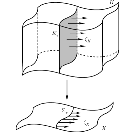
Figure 6.4: Infinitesimal slicings

An important special case arises when the spacetime $X$ is endowed with a Lorentzian metric $g$. Fix a spacelike hypersurface $\Sigma_{\tau}\subset X$ and let $e_{\perp}$ denote the future-pointing timelike unit normal vector field on $\Sigma_{\tau}$; then $(\Sigma_{\tau},e_{\perp})$ is an infinitesimal slicing of $X$. In coordinates adapted to $\Sigma_{\tau}$ we expand

$$\frac{\partial}{\partial x^{0}}=Ne_{\perp}+M^{i}\frac{\partial}{\partial x^{i}},$$ (6A.6)

where $N$ is a function on $\Sigma_{\tau}$ (the lapse) and ${\bf M}=M^{i}{\partial}/{\partial x^{i}}$ is a vector field tangent to $\Sigma_{\tau}$ (the shift). It is often useful to refer an arbitrary infinitesimal slicing $\zeta_{X}=\zeta^{\mu}\partial/\partial x^{\mu}$ to the frame $\{e_{\perp},\partial_{i}\}$, relative to which we have

$$\zeta_{X}=\zeta^{0}Ne_{\perp}+(\zeta^{0}M^{i}+\zeta^{i})\frac{\partial}{\partial x^{i}}.$$ (6A.7)

We remark that, in general, neither $\partial/\partial x^{0}$ nor $\zeta_{X}$ need be timelike.

In both our and ADM’s (Arnowitt, Deser, and Misner [1962]) formalisms, these lapse and shift functions play a key role. For instance, in the construction of spacetimes from initial data (say, using a computer), they are used to control the choice of slicing. This can be seen most clearly by imposing the ADM coordinate condition that $\partial/\partial x^{0}$ coincide with $\zeta_{X}$, in which case (6A.7) reduces simply to

$$\zeta_{X}=Ne_{\perp}+{\mathbf{M}}.$$ (6A.8)

 

a   Particle Mechanics.

Both $X=\mathbb{R}$ and $Y=\mathbb{R}\times Q$ for particle mechanics are “already sliced” with $\zeta_{X}={d}/{dt}$ and $\zeta_{Y}={\partial}/{\partial t}$ respectively. From the infinitesimal equivariance equation (4D.2), it follows that this slicing is Lagrangian relative to $\mathcal{L}=L(t,q^{A},v^{A})dt$ iff ${\partial L}/{\partial t}=0$, that is, $L$ is time-independent.

One can consider more general slicings of $X$, interpreted as diffeomorphisms $\mathfrak{s}_{X}:\mathbb{R}\to\mathbb{R}$. The induced slicing $\mathfrak{s}_{Y}:Q\times\mathbb{R}\to Y$ given by $\mathfrak{s}_{Y}(q^{1},\dots,q^{N},t)=(q^{1},\dots,q^{N},\mathfrak{s}_{X}(t))$ will be Lagrangian if $\mathcal{L}$ is time reparametrization-invariant.

We can be substantially more explicit for the relativistic free particle. Consider an arbitrary slicing $Q\times\mathbb{R}\to Y$ with generating vector field

$$\zeta_{Y}=\chi\frac{\partial}{\partial t}+\zeta^{A}\frac{\partial}{\partial q^{A}}.$$ (6A.9)

From (4D.2) we see that the slicing is Lagrangian relative to (3C.8) iff

$$g_{BC,A}v^{B}v^{C}\zeta^{A}+g_{AC}v^{C}\left(\frac{\partial\zeta^{A}}{\partial t}+v^{B}\frac{\partial\zeta^{A}}{\partial q^{B}}\right)=0.$$ (6A.10)

(The terms involving $\chi$ drop out as $\mathcal{L}$ is time reparametrization-invariant.) But (6A.10) holds for all $\mathbf{v}$ iff $\partial\zeta^{A}/\partial t=0$ and

$$0=g_{BC,A}v^{B}v^{C}\zeta^{A}+g_{AC}v^{C}v^{B}\frac{\partial\zeta^{A}}{\partial q^{B}}=v^{A}v^{B}\zeta_{(A;B)}.$$

Thus $\zeta^{A}\partial/\partial q^{A}$ must be a Killing vector field. It follows that the most general Lagrangian slicing consists of time reparametrizations horizontally and isometries vertically.

b   Electromagnetism.

Any slicing of the spacetime $X$ naturally induces a slicing of the bundle ${\tilde{Y}}=\Lambda^{1}X\times S^{\mspace{1.5mu}3,1}_{2}(X)$ by push-forward. If $\zeta_{X}=\zeta^{\mu}\partial/\partial x^{\mu}$, the generating vector field of this induced slicing is

$$\zeta_{\tilde{Y}}=\zeta^{\mu}\frac{\partial}{\partial x^{\mu}}-A_{\nu}\zeta^{\nu}_{\>\>\>,\alpha}\frac{\partial}{\partial A_{\alpha}}-(g_{\sigma\mu}\zeta^{\mu}_{\>\>\>,\rho}+g_{\rho\mu}\zeta^{\mu}_{\>\>\>,\sigma})\frac{\partial}{\partial g_{\sigma\rho}}.$$

The most general slicing of $\tilde{Y}$ replaces the coefficients of the second and third terms by $\chi_{\alpha}$ and $\chi_{\sigma\rho}$, respectively, where the $\chi$s are any functions on $\tilde{Y}$.

The restriction to $\mathcal{G}$-slicings, with $\mathcal{G}=\mbox{Diff}(X)\;\circledS\;\mathcal{F}(X)$ as in Example b of §4C, is not very severe for the parametrized version of Maxwell’s theory. Any complete vector field $\zeta_{X}=\zeta^{\mu}\partial/\partial x^{\mu}$ may be used as the generator of the spacetime slicing; then for the slicing of $\tilde{Y}$ we have the generator

$$\zeta_{\tilde{Y}}=\zeta^{\mu}\frac{\partial}{\partial x^{\mu}}+(\chi_{,\alpha}-A_{\nu}\zeta^{\nu}_{\>\>\>,\alpha})\frac{\partial}{\partial A_{\alpha}}-(g_{\sigma\mu}\zeta^{\mu}_{\>\>\>,\rho}+g_{\rho\mu}\zeta^{\mu}_{\>\>\>,\sigma})\frac{\partial}{\partial g_{\sigma\mspace{-1.5mu}\rho}},$$ (6A.11)

where $\chi$ is an arbitrary function on $X$ (generating a Maxwell gauge transformation). A more general Lagrangian slicing (which, however, is not a $\mathcal{G}$-slicing) is obtained from this upon replacing $\chi_{,\alpha}$ by the components of a closed 1-form on $X$.

On the other hand, if we work with electromagnetism on a fixed spacetime background, the $\zeta_{X}$ must be a Killing vector field of the background metric $g$, and $\zeta_{Y}$ is of the form (6A.11) with this restriction on $\zeta^{\mu}$ (and without the term in the direction $\partial/\partial g_{\sigma\rho}$.) If the background spacetime is Minkowskian, then $\zeta_{X}$ must be a generator of the Poincaré group. For a generic background spacetime, there are no Killing vectors, and hence no Lagrangian slicings. (This leads one to favor the parametrized theory.)

c   A Topological Field Theory.

With reference to Example b above, we see that with $\mathcal{G}=\mbox{Diff}(X)\;\circledS\;\mathcal{F}(X)$, a $\mathcal{G}$-slicing of $Y=\Lambda^{1}X$ is generated by

$$\zeta_{Y}=\zeta^{\mu}\frac{\partial}{\partial x^{\mu}}+(\chi_{,\alpha}-A_{\nu}\zeta^{\nu}_{\>\>\>,\alpha})\frac{\partial}{\partial A_{\alpha}}.$$ (6A.12)

Note that (6A.12) does not generate a Lagrangian slicing unless $\chi=0$, since the replacement $A\mapsto A+\mbox{\bf d}\chi$ does not leave the Chern–Simons Lagrangian density invariant (cf. §4D).

d   Bosonic Strings.

In this case the configuration bundle

$$Y=(X\times M)\times_{X}S^{1,1}_{2}(X)$$

is already sliced with $\zeta_{X}={\partial}/{\partial x^{0}}$ and $\zeta_{Y}={\partial}/{\partial x^{0}}$. More generally, one can consider slicings with generators of the form

$$\zeta^{\mu}\frac{\partial}{\partial x^{\mu}}+\zeta^{A}\frac{\partial}{\partial\phi^{A}}+\zeta_{\sigma p}\frac{\partial}{\partial h_{\sigma\mspace{-1.5mu}\rho}}.$$ (6A.13)

Such a slicing will be Lagrangian relative to the Lagrangian density (3C.23) iff $\zeta^{A}{\partial}/{\partial\phi^{A}}$ is a Killing vector field of $(M,g)$ (this works much the same way as Example a) and

$$\zeta_{\sigma\mspace{-1.5mu}\rho}=-(h_{\sigma\alpha}\zeta^{\alpha}{}{}_{,\rho}+h_{\rho\alpha}\zeta^{\alpha}{}_{,\sigma})+2\lambda h_{\sigma\mspace{-1.5mu}\rho}$$ (6A.14)

for some function $\lambda$ on $X$. The first two terms in this expression represent that “part” of the slicing which is induced by the slicing $\zeta_{X}$ of $X$ by push-forward, and the last term reflects the freedom to conformally rescale $h$ while leaving the harmonic map Lagrangian invariant. The slicing represented by (6A.13) will be a $\mathcal{G}$-slicing, with $\mathcal{G}=\operatorname{Diff}(X)\;\circledS\;\mbox{Con}^{1,1}_{2}(X)$, iff $\zeta^{A}=0$. $\blacklozenge$  $\blacklozenge$

6B Space + Time Decomposition of the Jet Bundle

In Chapter 5 we have space + time decomposed the multisymplectic formalism relative to a fixed Cauchy surface $\Sigma_{\tau}\in X$ to obtain the associated $\tau$-phase space $T^{*}\mathcal{Y}_{\tau}$ with its symplectic structure $\omega_{\tau}=-\mathbf{d}\theta_{\tau}$. Now we show how to perform a similar decomposition of the jet bundle $J^{1}Y$ using the notion of an infinitesimal slicing. Effectively, this enables us to invariantly separate the temporal from the spatial derivatives of the fields.

Fix an infinitesimal slicing $(Y_{\tau},\zeta:=\zeta_{Y})$ of $Y$ and set

$$\varphi:=\phi\!\bigm{|}\!\Sigma_{\tau}\quad\text{and}\quad\dot{\varphi}:=\pounds_{\zeta}\phi\!\bigm{|}\!\Sigma_{\tau},$$

so that in coordinates

$$\varphi^{A}=\phi^{A}\!\bigm{|}\!\Sigma_{\tau}\quad\text{and}\quad\dot{\varphi}^{A}=(\zeta^{\mu}\phi^{A}{}_{,\mu}-\zeta^{A}\circ\phi)\!\bigm{|}\!\Sigma_{\tau}.$$ (6B.1)

Define an affine bundle map $\beta_{\zeta}:(J^{1}Y)_{\tau}\to J^{1}(Y_{\tau})\times VY_{\tau}$ over $Y_{\tau}$ by

$$\beta_{\zeta}(j^{1}\mspace{-1.5mu}\phi(x))=(j^{1}\mspace{-1.5mu}\varphi(x),\dot{\varphi}(x))$$ (6B.2)

for $x\in\Sigma_{\tau}$. In coordinates adapted to $\Sigma_{\tau}$, (6B.2) reads

$$\beta_{\zeta}(x^{i},y^{A},v^{A}{}_{\mu})=(x^{i},y^{A},v^{A}{}_{j},\dot{y}^{A}).$$ (6B.3)

Furthermore, if the coordinates on $Y$ are arranged so that

$$\frac{\partial}{\partial x^{0}}\!\bigm{|}\!Y_{\tau}=\zeta,\quad\text{ then }\quad\dot{y}^{A}=v^{A}{}_{0}.$$

This last observation establishes:

Proposition 6.1.

If $\zeta_{X}$ is transverse to $\Sigma_{\tau}$, then $\beta_{\zeta}$ is an isomorphism.

The bundle isomorphism $\beta_{\zeta}$ is the jet decomposition map and its inverse the jet reconstruction map. Clearly, both can be extended to maps on sections; from (6B.2) we have

$$\beta_{\zeta}(j^{1}\mspace{-1.5mu}\phi\circ i_{\tau})=(j^{1}\mspace{-1.5mu}\varphi,\dot{\varphi})$$ (6B.4)

where $i_{\tau}:\Sigma_{\tau}\to X$ is the inclusion. In fact:

Corollary 6.2.

$\beta_{\zeta}$ induces an isomorphism of $(j^{1}\mathcal{Y})_{\tau}$ with $T\mathcal{Y}_{\tau}$, where $(j^{1}\mathcal{Y})_{\tau}$ is the collection of restrictions of holonomic sections of $J^{1}Y\to X$ to $\Sigma_{\tau}$.

• Since $\dot{\varphi}$ is a section of $VY_{\tau}$ covering $\varphi$, by (5A.1) it defines an element of $T_{\varphi}\mathcal{Y}_{\tau}$. The result now follows from the previous Proposition and the comment afterwards. ∎

One may wish to decompose $Y$, as well as $J^{1}Y$, relative to a slicing. This is done so that one works with fields that are spatially covariant rather than spacetime covariant. For example, in electromagnetism, sections of $Y=\Lambda^{1}X$ are one-forms $A=A_{\mu}dx^{\mu}$ over spacetime and sections of $Y_{\tau}=\Lambda^{1}X\!\bigm{|}\!\Sigma_{\tau}$ are spacetime one-forms restricted to $\Sigma_{\tau}$. One may split

$$Y_{\tau}=\Lambda^{1}\Sigma_{\tau}\times_{\Sigma_{\tau}}\Lambda^{0}\Sigma_{\tau},$$ (6B.5)

so that the instantaneous configuration space consists of spatial one-forms $\mathbf{A}=A_{m}dx^{m}$ together with spatial scalars $a$. The map $\Lambda^{1}X\!\bigm{|}\!\Sigma_{\tau}\to\Lambda^{1}\Sigma_{\tau}\times_{\Sigma_{\tau}}\Lambda^{0}\Sigma_{\tau}$ which effects this split takes the form

$$A\mapsto(\mathbf{A},a)$$ (6B.6)

where $a=i_{\tau}^{*}(\zeta_{X}\mathbin{\hbox to6.0pt{\vrule height=0.4pt,width=5.0pt,depth=0.0pt\kern-0.4pt\vrule height=6.0pt,width=0.4pt,depth=0.0pt\hss}}A)$ and $\mathbf{A}=i_{\tau}^{*}A$.

One particular case of interest is that of a metric tensor $g$ on $X$. Let $S^{\mspace{1.5mu}n,1}_{2}(X,\Sigma_{\tau})$ denote the subbundle of $S^{\mspace{1.5mu}n,1}_{2}(X)$ consisting of those Lorentz metrics on $X$ with respect to which $\Sigma_{\tau}$ is spacelike. We may space $+$ time split

$$S^{\mspace{1.5mu}n,1}_{2}(X,\Sigma_{\tau})\!\bigm{|}\!\Sigma_{\tau}=S^{\mspace{1.5mu}n}_{2}(\Sigma_{\tau})\times_{\Sigma_{\tau}}T\Sigma_{\tau}\times_{\Sigma_{\tau}}\Lambda^{0}\Sigma_{\tau}$$ (6B.7)

as follows (cf. §21.4 of Misner, Thorne, and Wheeler [1973]). Let $e_{\perp}$ the the forward-pointing unit timelike normal to $\Sigma_{\tau}$, and let $N,\mspace{1.5mu}{\bf M}$ be the lapse and shift functions defined via (6A.6). Set $\gamma=i_{\tau}^{*}g$, so that $\gamma$ is a Riemannian metric on $\Sigma_{\tau}.$ Then the decomposition $g\mapsto(\gamma,{\bf M},N)$ with respect to the infinitesimal slicing $(\Sigma_{\tau},e_{\perp})$ is given by

$$g=\gamma_{jk}(dx^{j}+M^{j}dt)(dx^{k}+M^{k}dt)-N^{2}dt^{2}$$

or, in terms of matrices,

$$\left(\begin{array}[]{cc}g_{00}&g_{0i}\\ &\\ g_{i0}&g_{jk}\end{array}\right)=\left(\begin{array}[]{cc}M_{k}M^{k}-N^{2}&M_{i}\\ &\\ M_{i}&\gamma_{jk}\end{array}\right).$$ (6B.8)

This decomposition has the corresponding contravariant form

$$g^{-1}=\gamma^{jk}\partial_{j}\partial_{k}-\frac{1}{N^{2}}(\partial_{t}-M^{j}\partial_{j})(\partial_{t}-M^{k}\partial_{k})$$

or, in terms of matrices,

$$\left(\begin{array}[]{cc}g^{00}&g^{0i}\\ &\\ g^{i0}&g^{jk}\end{array}\right)=\left(\begin{array}[]{cc}-1/N^{2}&M^{i}/N^{2}\\ &\\ M^{i}/N^{2}&\gamma^{jk}-M^{j}M^{k}/N^{2}\end{array}\right)$$ (6B.9)

where $M_{i}=\gamma_{ij}M^{j}.$ Furthermore, the metric volume $\sqrt{-g}$ decomposes as

$$\sqrt{-g}=N\sqrt{\gamma}.$$ (6B.10)

The dynamical analysis can by carried out whether or not these splits of the configuration space are done; it is largely a matter of taste. Later, in Chapters 12 and 13 when we discuss dynamic fields and atlas fields, these types of splits will play a key role.

6C The Instantaneous Legendre Transform

Using the jet reconstruction map we may space + time split the Lagrangian as follows. Define

$$\mathcal{L}_{\tau,\zeta}:J^{1}(Y_{\tau})\times VY_{\tau}\to\Lambda^{n}\Sigma_{\tau}$$

by

$$\mathcal{L}_{\tau,\zeta}(j^{1}\mspace{-1.5mu}\varphi(x),\dot{\varphi}(x))=i^{*}_{\tau}\mathbf{i}_{\zeta_{X}}\mathcal{L}(j^{1}\mspace{-1.5mu}\phi(x)),$$ (6C.1)

where $j^{1}\mspace{-1.5mu}\phi\circ i_{\tau}$ is the reconstruction of $(j^{1}\mspace{-1.5mu}\varphi,\dot{\varphi})$. The instantaneous Lagrangian $L_{\tau,\zeta}:T\mathcal{Y}_{\tau}\to\mathbb{R}$ is defined by

$$L_{\tau,\zeta}(\varphi,\dot{\varphi})=\int_{\Sigma_{\tau}}\mathcal{L}_{\tau,\zeta}(j^{1}\mspace{-1.5mu}\varphi,\dot{\varphi})$$ (6C.2)

for $(\varphi,\dot{\varphi})\in T\mathcal{Y}_{\tau}$ (cf. Corollary 6.2). In coordinates adapted to $\Sigma_{\tau}$ this becomes, with the aid of (6C.1) and (3A.1),

$$L_{\tau,\zeta}(\varphi,\dot{\varphi})=\int_{\Sigma_{\tau}}L(j^{1}\mspace{-1.5mu}\varphi,\dot{\varphi})\zeta^{0}d^{\mspace{1.5mu}n}\mspace{-1.5mu}x_{0}.$$ (6C.3)

The instantaneous Lagrangian $L_{\tau,\zeta}$ defines an instantaneous Legendre transform

$$\mathbb{F}L_{\tau,\zeta}:T\mathcal{Y}_{\tau}\to T^{*}\mathcal{Y}_{\tau};\quad(\varphi,\dot{\varphi})\mapsto(\varphi,\pi)$$ (6C.4)

in the usual way (cf. Abraham and Marsden [1978]). In adapted coordinates

$$\pi=\pi_{A}\,dy^{A}\otimes d^{\mspace{1.5mu}n}\mspace{-1.5mu}x_{0}$$

and (6C.4) reads

$$\pi_{A}=\frac{\partial\mathcal{L}_{\tau,\zeta}}{\partial\dot{y}^{A}}.$$ (6C.5)

We call

$$\mathcal{P}_{\tau,\zeta}=\operatorname{im}\mathbb{F}L_{\tau,\zeta}\subset T^{*}\mathcal{Y}_{\tau}$$

the instantaneous or $\tau$-primary constraint set.

A3  Almost Regularity

Assume that $\mathcal{P}_{\tau,\zeta}$ is a smooth, closed, submanifold of $T^{*}\mathcal{Y}_{\tau}$ and that $\mathbb{F}L_{\tau,\zeta}$ is a submersion with connected fibers.

• Assumption A3 is satisfied in cases of interest.

2.

We shall see momentarily that $\mathcal{P}_{\tau,\zeta}$ is independent of $\zeta$.

3.

In obtaining (6C.5) we use the fact that $\mathcal{L}$ is first order. See Gotay [1991] for a treatment of the higher order case.  $\blacklozenge$

We now investigate the relation between the covariant and instantaneous Legendre transformations. Recall that over $\mathcal{Y}_{\tau}$ we have the symplectic bundle map $R_{\tau}:(\mathcal{Z}_{\tau},\Omega_{\tau})\to(T^{*}\mathcal{Y}_{\tau},\omega_{\tau})$ given by

$$\langle R_{\tau}(\sigma),V\rangle=\int_{\Sigma_{\tau}}\varphi^{*}(\mathbf{i}_{V}\sigma)$$

where $\varphi=\pi_{Y\!Z}\circ\sigma$ and $V\in T_{\varphi}\mathcal{Y}_{\tau}$.

Proposition 6.3.

Assume $\zeta_{X}$ is transverse to $\Sigma_{\tau}$. Then the following diagram commutes:

$$\begin{CD}(j^{1}\mathcal{Y})_{\tau}@>{\mathbb{F}\mathcal{L}}>{}>\mathcal{Z}_{\tau}\\ @V{\beta_{\zeta}}V{}V@V{}V{R_{\tau}}V\\ T\mathcal{Y}_{\tau}@>{}>{\mathbb{F}L_{\tau,\zeta}}>T^{*}\mathcal{Y}_{\tau}\end{CD}$$ (6C.6)

• Choose adapted coordinates in which $\partial_{0}\!\bigm{|}\!Y_{\tau}=\zeta$. Since $R_{\tau}$ is given by $\pi_{A}=p_{A}{}^{0}\circ\sigma$, going clockwise around the diagram we obtain

  $$R_{\tau}\!\left(\mathbb{F}\mathcal{L}(j^{1}\mspace{-1.5mu}\phi\circ i_{\tau})\right)=\frac{\partial L}{\partial v^{A}{}_{0}}(\phi^{B},\phi^{B}{}_{,\mu})\mspace{1.5mu}dy^{A}\otimes d^{\mspace{1.5mu}n}\mspace{-1.5mu}x_{0}.$$

  This is the same as one gets going counterclockwise, taking into account (6B.3), (6C.5) and the fact that $\mathbb{F}L_{\tau,\zeta}$ is evaluated at $\dot{\varphi}^{A}=\phi^{A}{}_{,0}$. ∎

We define the covariant primary constraint set to be

$$N=\mathbb{F}\mathcal{L}(J^{1}Y)\subset Z$$

and with a slight abuse of notation, set

$$\mathcal{N}_{\tau}=\mathbb{F}\mathcal{L}\left((j^{1}\mathcal{Y})_{\tau}\right)\subset\mathcal{Z}_{\tau}.$$

Corollary 6.4.

If $\zeta_{X}$ is transverse to $\Sigma_{\tau}$, then

$$R_{\tau}(\mathcal{N}_{\tau})=\mathcal{P}_{\tau,\zeta}.$$ (6C.7)

In particular, $\mathcal{P}_{\tau,\zeta}$ is independent of $\zeta$, and so can be denoted simply $\mathcal{P}_{\tau}$.

• By Corollary 6.2, $\beta_{\zeta}$ is onto $T\mathcal{Y}_{\tau}$. The result now follows from the commutative diagram (6C.6). ∎

Denote by the same symbol $\omega_{\tau}$ the pullback of the symplectic form on $T^{*}\mathcal{Y}_{\tau}$ to the submanifold $\mathcal{P}_{\tau}$. When there is any danger of confusion we will write $\omega_{T^{*}\mathcal{Y}_{\tau}}$ and $\omega_{\mathcal{P}_{\tau}}$. In general $(\mathcal{P}_{\tau},\omega_{\tau})$ will be merely presymplectic. However, the fact that $\mathbb{F}L_{\tau,\zeta}$ is fiber-preserving together with the almost regularity assumption A3 imply that $\ker\omega_{\tau}$ is a regular distribution on $\mathcal{P}_{\tau}$ (in the sense that it defines a subbundle of $T\mathcal{P}_{\tau}$).

As always, the instantaneous Hamiltonian is given by

$$H_{\tau,\zeta}(\varphi,\pi)=\langle\pi,\dot{\varphi}\rangle-L_{\tau,\zeta}(\varphi,\dot{\varphi})$$ (6C.8)

and is defined only on $\mathcal{P}_{\tau}$. The density for $H_{\tau,\zeta}$ is denoted by $\mathfrak{H}_{\tau,\zeta}$. We remark that to determine a Hamiltonian, it is essential to specify a time direction $\zeta$ on $Y$. This is sensible, since the system cannot evolve without knowing what “time” is. For $\zeta_{Y}=\xi_{Y}$, where $\xi\in\mathfrak{g}$, the Hamiltonian will turn out to be the negative of the energy-momentum map induced on $\mathcal{P}_{\tau}$ (cf. §7F). A crucial step in establishing this relationship is the following result:

Proposition 6.5.

Let $(\varphi,\pi)\in\mathcal{P}_{\tau}$. Then for any holonomic lift $\sigma$ of $(\varphi,\pi)$,

$$H_{\tau,\zeta}(\varphi,\pi)=-\int_{\Sigma_{\tau}}\sigma^{*}(\mathbf{i}_{\zeta_{Z}}\Theta).$$ (6C.9)

Here $\zeta_{Z}$ is the canonical lift of $\zeta$ to $Z$ (cf. §4B). By a holonomic lift of $(\varphi,\pi)$ we mean any element $\sigma\in R^{-1}_{\tau}\{(\varphi,\pi)\}\cap\mathcal{N}_{\tau}$. Holonomic lifts of elements of $\mathcal{P}_{\tau}$ always exist by virtue of Proposition 6.3.

• We will show that (6C.9) holds on the level of densities; that is,

  $$\mathfrak{H}_{\tau,\zeta}(\varphi,\pi)=-\sigma^{*}(\mathbf{i}_{\zeta_{Z}}\Theta).$$ (6C.10)

  Using adapted coordinates, (2B.11) yields

  $$\sigma^{*}(\mathbf{i}_{\zeta_{Z}}\Theta)=\\[6.45831pt] \left\{(p_{A}{}^{0}\circ\sigma)\left(\zeta^{A}\circ\sigma-\zeta^{\mu}\sigma^{A}{}_{,\mu}\right)+\left(p\circ\sigma+(p_{A}{}^{\mu}\circ\sigma)\sigma^{A}{}_{,\mu}\right)\zeta^{0}\right\}d^{\mspace{1.5mu}n}\mspace{-1.5mu}x_{0}$$

  for any $\sigma\in\mathcal{Z}_{\tau}$. Now suppose that $(\varphi,\pi)\in\mathcal{P}_{\tau}$, and let $\sigma$ be any lift of $(\varphi,\pi)$ to $\mathcal{N}_{\tau}$. Thus, there is a $\phi\in\mathcal{Y}$ with $\mathbb{F}\mathcal{L}\circ j^{1}\mspace{-1.5mu}\phi\circ i_{\tau}=\sigma$. Then, using (3A.2), (6B.1), (5D.4) and (6C.1), the above becomes

  $$\sigma^{*}(\mathbf{i}_{\zeta_{Z}}\Theta)=-\pi(\dot{\varphi})+L(j^{1}\mspace{-1.5mu}\phi)\zeta^{0}\,d^{\mspace{1.5mu}n}\mspace{-1.5mu}x_{0}=-\pi(\dot{\varphi})+\mathcal{L}_{\tau,\zeta}(\varphi,\dot{\varphi}).$$ ∎

Notice that (6C.9) and (6C.10) are manifestly linear in $\zeta_{Z}$. This linearity foreshadows the linearity of the Hamiltonian (1.2) in the “atlas fields” to which we alluded in the introduction.

 

a   Particle Mechanics.

First consider a nonrelativistic particle Lagrangian of the form

$$L(q,v)=\frac{1}{2}g_{AB}(q)v^{A}v^{B}+V(q).$$

Taking $\zeta={\partial}/{\partial t}$, the Legendre transformation gives $\pi_{A}=g_{AB}(q)v^{B}$. If $g_{AB}(q)$ is invertible for all $q$, then $\mathbb{F}L_{t}$ is onto for each $t$ and there are no primary constraints.

For the relativistic free particle, the covariant primary constraint set $N\subset Z$ is determined by the constraints

$$g^{AB}p_{A}p_{B}=-m^{2}\qquad\text{and}\qquad p=0,$$ (6C.11)

which follow from (3C.10).

Now fix any infinitesimal slicing

$$\left(Y_{t},\zeta=\chi\frac{\partial}{\partial t}+\zeta^{A}\frac{\partial}{\partial q^{A}}\right)$$

of $Y$. Then we may identify $(J^{1}Y)_{t}$ with $TQ$ according to (6B.2); that is,

$$(q^{A},v^{A})\mapsto(q^{A},\dot{q}^{A})$$

where $\dot{q}^{A}=\chi v^{A}-\zeta^{A}$. The instantaneous Lagrangian (6C.2) is then

$$L_{t,\zeta}(q,\dot{q})=-m\|\dot{\mathbb{q}}+{\boldsymbol{\zeta}}\|$$ (6C.12)

(provided we take $\chi>0$). The instantaneous Legendre transform (6C.4) gives

$$\pi_{A}=\frac{mg_{AB}(\dot{q}^{B}+\zeta^{B})}{\|\dot{\mathbb{q}}+{\boldsymbol{\zeta}}\|}.$$ (6C.13)

The $t$-primary constraint set is then defined by the “mass constraint”

$$g^{AB}\pi_{A}\pi_{B}=-m^{2}.$$ (6C.14)

Comparing (6C.14) with (6C.11) we verify that $\mathcal{P}_{t}=R_{t}(\mathcal{N}_{t})$ as predicted by (6C.7). Using (6C.14) and (6C.8) we compute

$$H_{t,\zeta}(q,\pi)=-\zeta^{A}\pi_{A}.$$ (6C.15)

Looking ahead to Part III (cf. also the Introduction and Remark 9 of §6E), it may seem curious that $H_{t,\zeta}$ does not vanish identically, since after all the relativistic free particle is a parametrized system. This is because the slicing generated by (6A.9) is not a $\mathcal{G}$-slicing unless $\zeta^{A}=0$, in which case the Hamiltonian does vanish.

b   Electromagnetism.

First we consider the parametrized case. Let $\Sigma_{\tau}$ be a spacelike hypersurface locally given by $x^{0}=$ constant, and consider the infinitesimal $\mathcal{G}$-slicing $({\tilde{Y}}_{\tau},\zeta)$ with $\zeta$ given by (6A.11):

$$\hskip 28.0pt\zeta_{\tilde{Y}}=\zeta^{\mu}\frac{\partial}{\partial x^{\mu}}+(\chi_{,\alpha}-A_{\nu}\zeta^{\nu}_{\>\>\>,\alpha})\frac{\partial}{\partial A_{\alpha}}-(g_{\sigma\mu}\zeta^{\mu}_{\>\>\>,\rho}+g_{\rho\mu}\zeta^{\mu}_{\>\>\>,\sigma})\frac{\partial}{\partial g_{\sigma\rho}}.$$

We construct the instantaneous Lagrangian $L_{\tau,\zeta}$. From (6B.1) we have

$$\dot{A}_{\mu}=\zeta^{0}A_{\mu,0}+\zeta^{i}A_{\mu,i}-(\chi_{,\mu}-A_{\nu}\zeta^{\nu}_{\>\>\>,\mu}),$$ (6C.16)

and so (3C.13) gives in particular

$$F_{0i}=\frac{1}{\zeta^{0}}\left(\dot{A}_{i}-\zeta^{k}A_{i,k}+\chi_{,i}-A_{\nu}\zeta^{\nu}_{\>\>\>,i}-\zeta^{0}A_{0,i}\right).$$ (6C.17)

Substituting this into (3C.12), (6C.3) yields

$$L_{\tau,\zeta}(A,\dot{A};g) = \int_{\Sigma_{\tau}}\bigg{[}\frac{1}{2\zeta^{0}}(g^{i0}g^{j0}-g^{ij}g^{00})$$ (6C.18)

$$\hskip 20.66663pt\mbox{}\times(\dot{A}_{i}-\zeta^{k}A_{i,k}+\chi_{,i}-A_{\nu}\zeta^{\nu}_{\>\>\>,i}-\zeta^{0}A_{0,i})$$

$$\hskip 20.66663pt\mbox{}\times(\dot{A}_{j}-\zeta^{m}A_{j,m}+\chi_{,j}-A_{\rho}\zeta^{\rho}_{\>\>\>,j}-\zeta^{0}A_{0,j})$$

$$\hskip 20.66663pt\mbox{}+g^{ik}g^{0m}(\dot{A}_{i}-\zeta^{k}A_{i,k}+\chi_{,i}-A_{\nu}\zeta^{\nu}_{\>\>\>,i}-\zeta^{0}A_{0,i})F_{km}$$

$$\hskip 20.66663pt\mbox{}-\frac{1}{4}g^{ik}g^{jm}F_{ij}F_{km}\zeta^{0}\bigg{]}\sqrt{-g}\,d^{\mspace{1.5mu}3}\mspace{-1.5mu}x_{0}.$$

The corresponding instantaneous Legendre transformation $\mathbb{F}L_{\tau,\zeta}$ is defined by

$${\mathfrak{E}}^{i} = \bigg{(}\frac{1}{\zeta^{0}}(g^{i0}g^{j0}-g^{ij}g^{00})(\dot{A}_{j}-\zeta^{m}A_{j,m}+\chi_{,j}-A_{\rho}\zeta^{\rho}_{\>\>\>,j}-\zeta^{0}A_{0,j})$$ (6C.19)

$$\hskip 10.33331pt\mbox{}+g^{ik}g^{0m}F_{km}\bigg{)}\sqrt{-g}$$

and

$${\mathfrak{E}}^{0}=0.$$ (6C.20)

This last relation is the sole primary constraint in the Maxwell theory. Thus the $\tau$-primary constraint set is

$$\tilde{\mathcal{P}}_{\tau}=\big{\{}(A,\mathfrak{E};g)\in T^{*}{{\mathcal{Y}}}_{\tau}\times\big{(}{\mathcal{S}}^{3,1}_{2}\big{)}_{\tau}\,\big{|}\,\mathfrak{E}^{0}=0\big{\}}.$$ (6C.21)

It is clear that the almost regularity assumption A3 is satisfied in this case, and that $\tilde{\mathcal{P}}_{\tau}$ is indeed independent of the choice of $\zeta$ as required by Corollary 6.4. Using (3C.14) and (5D.6), one can also verify that (6C.19) and (6C.20) are consistent with the covariant Legendre transformation. In particular, the primary constraint $\mathfrak{E}^{0}=0$ is a consequence of the relation $\mathfrak{E}^{\nu}=\mathfrak{F}^{\nu 0}$ together with the fact that $\mathfrak{F}^{\nu\mu}$ is antisymmetric on $N$.

Taking (6C.20) into account, (5D.7) yields the presymplectic form

$$\omega_{\tau}(A,\mathfrak{E};g)=\int_{\Sigma_{\tau}}(dA_{i}\wedge d\mathfrak{E}^{i})\otimes d^{\mspace{1.5mu}3}\mspace{-1.5mu}x_{0}$$ (6C.22)

on $\tilde{\mathcal{P}}_{\tau}$. The Hamiltonian on $\tilde{\mathcal{P}}_{\tau}$ is obtained by solving (6C.19) for $\dot{A}_{i}$ and substituting into (6C.8). After some effort, we obtain

$$H_{\tau,\zeta}(A,\mathfrak{E};g) =\int_{\Sigma_{\tau}}\bigg{[}\zeta^{0}N\gamma^{-1/2}\Big{(}\frac{1}{2}\gamma_{ij}\mathfrak{E}^{i}\mathfrak{E}^{j}+\frac{1}{4N^{2}}\gamma^{ik}\gamma^{jm}\mathfrak{F}_{ij}\mathfrak{F}_{km}\Big{)}$$

$$\qquad\mbox{}+\frac{1}{N\sqrt{\gamma}}(\zeta^{0}M^{i}+\zeta^{i})\mathfrak{E}^{j}\mathfrak{F}_{ij}+(\zeta^{\mu}A_{\mu}-\chi)_{,i}\mathfrak{E}^{i}\bigg{]}d^{\mspace{1.5mu}3}\mspace{-1.5mu}x_{0}$$ (6C.23)

where we have made use of the splitting (6B.8)–(6B.10) of the metric $g$. Note the appearance of the combination $\zeta^{\mu}A_{\mu}-\chi$ in (6C). Later we will recognize this as the “atlas field” for the parametrized version of Maxwell’s theory. Note also the presence of the characteristic combinations $\zeta^{0}N$ and $(\zeta^{0}M^{i}+\zeta^{i})$ originating from (6A.7).

For electromagnetism on a fixed spacetime background, the preceding computations must be modified slightly. For definiteness, we assume that $(X,g)$ is Minkowski spacetime $(\mathbb{R}^{4},\eta)$, and that $\Sigma_{\tau}$ is a spacelike hyperplane $x^{0}=$ constant. The main difference is that we must now require $\zeta_{X}$ to be a Poincaré generator. Again for definiteness, we suppose that $\zeta_{X}=\partial/\partial x^{0}$. Thus the slicing generator $\zeta_{\tilde{Y}}$ is replaced by

$$\zeta_{Y}=\frac{\partial}{\partial x^{0}}+\chi_{,\alpha}\frac{\partial}{\partial A_{\alpha}}.$$ (6C.24)

The computations above remain valid upon replacing $(\zeta^{0},\mbox{\boldmath{$\zeta$}})$ by $(1,{\bf 0})$. The Hamiltonian in this case reduces to

$$H_{\tau,(1,{\bf 0})}(A,\mathfrak{E})=\int_{\Sigma_{\tau}}\bigg{[}\frac{1}{2}\mathfrak{E}_{i}\mathfrak{E}^{i}+\frac{1}{4}\mathfrak{F}_{ij}\mathfrak{F}^{ij}+(A_{0}-\chi)_{,i}\mathfrak{E}^{i}\bigg{]}d^{\mspace{1.5mu}3}\mspace{-1.5mu}x_{0}.$$ (6C.25)

c  A Topological Field Theory.

Let $\Sigma_{\tau}$ be any compact surface in $X$, and fix the Lagrangian slicing

$$\zeta=\zeta^{\mu}\frac{\partial}{\partial x^{\mu}}-A_{\nu}\zeta^{\nu}_{\>\>\>,\alpha}\frac{\partial}{\partial A_{\alpha}}$$ (6C.26)

as in Example c of §6A. The computations are similar those in Example b above. In particular, (6C.16) and (6C.17) remain valid (with $\chi=0$). Together with (3C.18), these yield

$$L_{\tau,\zeta}(A,\dot{A})=\\[10.33331pt] \int_{\Sigma_{\tau}}\epsilon^{0ij}\bigg{(}(\dot{A}_{i}-\zeta^{k}A_{i,k}-A_{\nu}\zeta^{\nu}_{\>\>\>,i}-\zeta^{0}A_{0,i})A_{j}+\frac{1}{2}F_{ij}A_{0}\zeta^{0}\bigg{)}d^{\mspace{1.5mu}2}\mspace{-1.5mu}x_{0}.$$ (6C.27)

The instantaneous Legendre transformation is

$$\pi^{i}=\epsilon^{0ij}A_{j}\qquad\mbox{and}\qquad\pi^{0}=0;$$ (6C.28)

compare (3C.19). In contrast to electromagnetism, all of these relations are primary constraints. Thus the instantaneous primary constraint set is

$$\mathcal{P}_{\tau}=\left\{(A,\pi)\in T^{*}{{\mathcal{Y}}}_{\tau}\mid\pi^{0}=0\>\mbox{ and }\>\pi^{i}=\epsilon^{0ij}A_{j}\right\}.$$ (6C.29)

Again we see that the regularity assumption A3 is satisfied. From (6C.28) and (5D.9) we obtain the presymplectic form on $\mathcal{P}_{\tau}$,

$$\omega_{\tau}(A,\pi)=\int_{\Sigma_{\tau}}\big{(}\epsilon^{0ij}dA_{i}\wedge dA_{j}\big{)}\otimes d^{\mspace{1.5mu}2}\mspace{-1.5mu}x_{0}.$$ (6C.30)

The Chern-Simons Hamiltonian is

$$H_{\tau,\zeta}(A,\pi)=\int_{\Sigma_{\tau}}\epsilon^{0ij}\bigg{(}\zeta^{k}F_{ki}A_{j}-\frac{1}{2}\zeta^{0}F_{ij}A_{0}+(\zeta^{\mu}A_{\mu})_{,i}A_{j}\bigg{)}d^{\mspace{1.5mu}2}\mspace{-1.5mu}x_{0},$$ (6C.31)

which is consistent with (6C.9).

d   Bosonic Strings.

Consider an infinitesimal slicing $(\Sigma_{\tau},\zeta)$ as in (6A.13), with $\zeta^{A}=0$. (Here we must also suppose that the pull-back of $h$ to $\Sigma_{\tau}$ is positive-definite.) Using (6B.1) and (3C.23) the instantaneous Lagrangian turns out to be

$$L_{\tau,\zeta}(\varphi,h,\dot{\varphi},\dot{h})=-\frac{1}{2}\int_{\Sigma_{\tau}}\sqrt{|h|}\,g_{AB}\! \left(\frac{1}{\zeta^{0}}h^{00}(\dot{\varphi}^{A}\right.-\zeta^{1}\partial\varphi^{A})(\dot{\varphi}^{B}-\zeta^{1}\partial\varphi^{B})$$

$$\quad+2h^{01}(\dot{\varphi}^{A}-\zeta^{1}\partial\varphi^{A})\partial\varphi^{B}$$

$$\quad+\zeta^{0}h^{11}\biggl{.}\partial\varphi^{A}\partial\varphi^{B}\biggl{)}d^{\mspace{1.5mu}1}\mspace{-1.5mu}x_{0},$$ (6C.32)

where we have set $\partial\varphi^{A}:=\varphi^{A}{}_{,1}$. From this it follows that the instantaneous momenta are

$$\pi_{A}={-}\sqrt{|h|}\,g_{AB}\bigg{(}\frac{1}{\zeta^{0}}h^{00}(\dot{\varphi}^{B}-\zeta^{1}\partial\varphi^{B})+h^{01}\partial\varphi^{B}\bigg{)}$$ (6C.33)

$$\rho^{\sigma\mspace{-1.5mu}\rho}=0.$$ (6C.34)

Thus

$$\mathcal{P}_{\tau}=\left\{(\varphi,h,\pi,\rho)\in T^{*}\mathcal{Y}_{\tau}\bigm{|}\rho^{\sigma\mspace{-1.5mu}\rho}=0\right\}.$$ (6C.35)

This is consistent with (3C.24) and (3C.25) via (5D.10). A short computation then gives

$$H_{\tau,\zeta}(\varphi,h,\pi,\rho)=\\[7.74998pt] -\int_{\Sigma_{\tau}}\left(\frac{1}{2}|h|^{-1/2}\frac{1}{h^{00}}\zeta^{0}(\pi^{2}+\partial\varphi^{2})+\left(\frac{h^{01}}{h^{00}}\zeta^{0}-\zeta^{1}\right)(\pi\cdot\partial\varphi)\right)d^{\mspace{1.5mu}1}\mspace{-1.5mu}x_{0}$$

for the instantaneous Hamiltonian on $\mathcal{P}_{\tau}$, where we have used the abbreviations $\pi^{2}:=g^{AB}\pi_{A}\pi_{B}$ and $\pi\cdot\partial\varphi:=\pi_{A}\partial\varphi^{A}$, etc. If we space $+$ time split the metric $h$ as in (6B.8)–(6B.10), then the Hamiltonian becomes simply

$$H_{\tau,\zeta}(\varphi,h,\pi,\rho)=\\[7.74998pt] \int_{\Sigma_{\tau}}\left(\frac{1}{2\sqrt{\gamma}}\zeta^{0}N(\pi^{2}+\partial\varphi^{2})+(\zeta^{0}M+\zeta^{1})(\pi\cdot\partial\varphi)\right)d^{\mspace{1.5mu}1}\mspace{-1.5mu}x_{0}.$$ (6C.36)

This expression should be compared with its counterpart in ADM gravity, cf. Interlude III and Arnowitt, Deser, and Misner [1962]. In §12C we will identify $\zeta^{0}N$ and $\zeta^{0}M+\zeta^{1}$ as the “atlas fields” for the bosonic string.

Finally, using (6C.33) and (6C.34) in (5D.11), the presymplectic structure on $\mathcal{P}_{\tau}$ is

$$\quad\qquad\qquad\qquad\omega_{\tau}(\varphi,h,\pi,\rho)=\int_{\Sigma_{\tau}}(d\varphi^{A}\wedge d\pi_{A})\otimes d^{\mspace{1.5mu}2}\mspace{-1.5mu}x_{0}.\qquad\qquad\blacklozenge$$ (6C.37)

 

6D Hamiltonian Dynamics

We have now gathered together the basic ingredients of Hamiltonian dynamics: for each Cauchy surface $\Sigma_{\tau}$, we have the $\tau$-primary constraint set $\mathcal{P}_{\tau}$, a presymplectic structure $\omega_{\tau}$ on $\mathcal{P}_{\tau}$, and a Hamiltonian $H_{\tau,\zeta}$ on $\mathcal{P}_{\tau}$ relative to a choice of evolution direction $\zeta$. If we think of some fixed $\Sigma_{\tau}$ as the “initial time,” then fields $(\varphi,\pi)\in\mathcal{P}_{\tau}$ are candidate initial data for the $(n+1)$-decomposed field equations; that is, Hamilton’s equations. To evolve this initial data, we slice spacetime and the bundles over it into global moments of time $\lambda$.

To this end, we regard $\operatorname{Emb}(\Sigma,X)$ as the space of all (parametrized) Cauchy surfaces in the $(n+1)$-dimensional “spacetime” $X$. The arena for Hamiltonian dynamics in the instantaneous or $(n+1)$-formalism is the “instantaneous primary constraint bundle” $\mathcal{P}^{\Sigma}$ over $\operatorname{Emb}(\Sigma,X)$ whose fiber above $\tau\in\operatorname{Emb}(\Sigma,X)$ is $\mathcal{P}_{\tau}$.

Fix compatible slicings $\mathfrak{s}_{Y}$ and $\mathfrak{s}_{X}$ of $Y$ and $X$ with generating vector fields $\zeta$ and $\zeta_{X}$, respectively. As in §6A, let $\tau:\mathbb{R}\to\operatorname{Emb}(\Sigma,X)$ be the curve of embeddings defined by $\tau(\lambda)(x)=\mathfrak{s}_{X}(x,\lambda)$.

Let $\mathcal{P}^{\tau}$ denote the portion of $\mathcal{P}^{\Sigma}$ lying over the image of $\tau$ in $\operatorname{Emb}(\Sigma,X)$. Dynamics relative to the chosen slicing takes place in $\mathcal{P}^{\tau}$; we view the $(n+1)$-evolution of the fields as being given by a curve

$$c(\lambda)=(\varphi(\lambda),\pi(\lambda))$$

in $\mathcal{P}^{\tau}$ covering $\tau(\lambda)$. All this is illustrated in Figure 6-5.

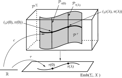
Figure 6.5: Instantaneous Dynamics

Our immediate task is to obtain the $(n+1)$-decomposed field equations on $\mathcal{P}^{\tau}$, which determine the curve $c(\lambda)$. This requires setting up a certain amount of notation.

Recall from §6A that the slicing $\mathfrak{s}_{Y}$ of $Y$ gives rise to a trivialization $\mathfrak{s}_{\mathcal{Y}}$ of $\mathcal{Y}^{\tau}$, and hence induces trivializations $\mathfrak{s}_{j^{1}\mspace{-1.5mu}\mathcal{Y}}$ of $(j^{1}\mathcal{Y})^{\tau}$ by jet prolongation and $\mathfrak{s}_{\mathcal{Z}}$ of $\mathcal{Z}^{\tau}$ and $\mathfrak{s}_{T^{*}\mspace{-1.5mu}\mathcal{Y}}$ of $T^{*}\mathcal{Y}^{\tau}$ by pull-back. These latter trivializations are therefore presymplectic and symplectic; that is, the associated flows restrict to presymplectic and symplectic isomorphisms on fibers respectively. Furthermore, the reduction maps $R_{\tau(\lambda)}:\mathcal{Z}_{\tau(\lambda)}\to T^{*}\mathcal{Y}_{\tau(\lambda)}$ intertwine the trivializations $\mathfrak{s}_{\mathcal{Z}}$ and $\mathfrak{s}_{T^{*}\mathcal{Y}}$ in the obvious sense.

Assume A2, viz., the slicing $\mathfrak{s}_{Y}$ of $Y$ is Lagrangian. From Proposition 4.6(i) $\mathbb{F}\mathcal{L}:(j^{1}\mathcal{Y})^{\tau}\to\mathcal{Z}^{\tau}$, regarded as a map on sections, is equivariant with respect to the (flows corresponding to the) induced trivializations of these spaces. (Infinitesimally, this is equivalent to the statement $T\mathbb{F}\mathcal{L}\cdot\zeta_{j^{1}\mspace{-1.5mu}\mathcal{Y}}=\zeta_{\mathcal{Z}}$ where $\zeta_{j^{1}\mspace{-1.5mu}\mathcal{Y}}$ and $\zeta_{\mathcal{Z}}$ are the generating vector fields of the trivializations.) This observation, combined with the above remarks on reduction, Proposition 6.3, and assumption A3, show that $\mathcal{P}^{\tau}$ really is a subbundle of $T^{*}\mathcal{Y}^{\tau}$, and that the symplectic trivialization $\mathfrak{s}_{T^{*}\mspace{-1.5mu}\mathcal{Y}}$ on $T^{*}\mathcal{Y}^{\tau}$ restricts to a presymplectic trivialization $\mathfrak{s}_{\mathcal{P}}$ of $\mathcal{P}^{\tau}$. We use this trivialization to coordinatize $\mathcal{P}^{\tau}$ by $(\varphi,\pi,\lambda)$. The vector field $\zeta_{\mathcal{P}}$ which generates this trivialization is transverse to the fibers of $\mathcal{P}^{\tau}$ and satisfies ${\zeta_{\mathcal{P}}}\mathbin{\hbox to6.0pt{\vrule height=0.4pt,width=5.0pt,depth=0.0pt\kern-0.4pt\vrule height=6.0pt,width=0.4pt,depth=0.0pt\hss}}\,d\lambda=1$. To avoid a plethora of indices (and in keeping with the notation of §6A), we will henceforth denote the fiber $\mathcal{P}_{\tau(\lambda)}$ of $\mathcal{P}^{\tau}$ over $\tau(\lambda)\in\operatorname{Emb}(\Sigma,X)$ simply by $\mathcal{P}_{\lambda}$, the presymplectic form $\omega_{\tau(\lambda)}$ by $\omega_{\lambda}$, etc.

Using $\zeta_{\mathcal{P}}$, we may extend the forms $\omega_{\lambda}$ along the fibers $\mathcal{P}_{\lambda}$ to a (degenerate) 2-form $\omega$ on $\mathcal{P}^{\tau}$ as follows. At any point $(\varphi,\pi)\in\mathcal{P}_{\lambda}$, set

$$\omega(\mathcal{V},\mathcal{W})=\omega_{\lambda}(\mathcal{V},\mathcal{W}),$$ (6D.1)

$$\omega(\zeta_{\mathcal{P}},\cdot)=0,$$ (6D.2)

where $\mathcal{V},\mathcal{W}$ are vertical vectors on $\mathcal{P}^{\tau}$ (i.e., tangent to $\mathcal{P}_{\lambda}$) at $(\varphi,\pi)$. Since $\mathcal{P}_{\lambda}$ has codimension one in $\mathcal{P}^{\tau}$, (6D.1) and (6D.2) uniquely determine $\omega$. It is closed since $\omega_{\lambda}$ is and since the trivialization generated by $\zeta_{\mathcal{P}}$ is presymplectic (in other words, $\pounds_{\zeta_{\mathcal{P}}}\omega=0$; cf. Gotay, Lashof, Śniatycki, and Weinstein [1983]).

Similarly, we define the function $H_{\zeta}$ on $\mathcal{P}^{\tau}$ by

$$H_{\zeta}(\varphi,\pi,\lambda)=H_{\lambda,\zeta}(\varphi,\pi).$$ (6D.3)

Tracing back through the definitions (6C.1) and (6C.2) of the instantaneous Lagrangian $L_{\lambda,\zeta}$, we find the condition that the slicing be Lagrangian guarantees that the function $L_{\zeta}:T\mathcal{Y}^{\tau}\to\mathbb{R}$ defined by

$$L_{\zeta}(\varphi,\dot{\varphi},\lambda)=L_{\lambda,\zeta}(\varphi,\dot{\varphi})$$

is independent of $\lambda$. Therefore, if A2 holds, (6C.8) implies that $\zeta_{\mathcal{P}}[H_{\zeta}]=0$.

Consider the 2-form $\omega+\mathbf{d}H_{\zeta}\wedge\mathbf{d}\lambda$ on $\mathcal{P}^{\tau}$. By construction,

$$\pounds_{\zeta_{\mathcal{P}}}(\omega+\mathbf{d}H_{\zeta}\wedge\mathbf{d}\lambda)=0.$$ (6D.4)

We say that a curve $c:\mathbb{R}\to\mathcal{P}^{\tau}$ is a dynamical trajectory provided $c(\lambda)$ covers $\tau(\lambda)$ and its $\lambda$-derivative $\dot{c}$ satisfies

$$\dot{c}\mathbin{\hbox to6.0pt{\vrule height=0.4pt,width=5.0pt,depth=0.0pt\kern-0.4pt\vrule height=6.0pt,width=0.4pt,depth=0.0pt\hss}}(\omega+\mathbf{d}H_{\zeta}\wedge\mathbf{d}\lambda)=0.$$ (6D.5)

The terminology is justified by the following result, which shows that (6D.5) is equivalent to Hamilton’s equations. First note that the tangent $\dot{c}$ to any curve $c$ in $\mathcal{P}^{\tau}$ covering $\tau$ can be uniquely split as

$$\dot{c}=X+\zeta_{\mathcal{P}}$$ (6D.6)

where $X$ is vertical in $\mathcal{P}^{\tau}$. Set $X_{\lambda}=X\!\bigm{|}\!\mathcal{P}_{\lambda}$.

Proposition 6.6.

A curve $c$ in $\mathcal{P}^{\tau}$ is a dynamical trajectory iff Hamilton’s equations

$$X_{\lambda}\mathbin{\hbox to6.0pt{\vrule height=0.4pt,width=5.0pt,depth=0.0pt\kern-0.4pt\vrule height=6.0pt,width=0.4pt,depth=0.0pt\hss}}\,\omega_{\lambda}=\mathbf{d}H_{\lambda,\zeta}$$ (6D.7)

hold at $c(\lambda)$ for every $\lambda\in\mathbb{R}$.

• With $\dot{c}$ as in (6D.6), we compute

  $$\dot{c}\mathbin{\hbox to6.0pt{\vrule height=0.4pt,width=5.0pt,depth=0.0pt\kern-0.4pt\vrule height=6.0pt,width=0.4pt,depth=0.0pt\hss}}\,(\omega+\mathbf{d}H_{\zeta}\wedge\mathbf{d}\lambda)=(X\mathbin{\hbox to6.0pt{\vrule height=0.4pt,width=5.0pt,depth=0.0pt\kern-0.4pt\vrule height=6.0pt,width=0.4pt,depth=0.0pt\hss}}\,\omega-\mathbf{d}H_{\zeta})+(X[H_{\zeta}]+\zeta_{\mathcal{P}}[H_{\zeta}])\,d\lambda.$$ (6D.8)

  A one-form $\alpha$ on $\mathcal{P}^{\tau}$ is zero iff the pull-back of $\alpha$ to each $\mathcal{P}_{\lambda}$ vanishes and $\alpha(\zeta_{\mathcal{P}})=0$. Applying this to (6D.8) gives

  $$X_{\lambda}\mathbin{\hbox to6.0pt{\vrule height=0.4pt,width=5.0pt,depth=0.0pt\kern-0.4pt\vrule height=6.0pt,width=0.4pt,depth=0.0pt\hss}}\,\omega_{\lambda}=\mathbf{d}H_{\lambda,\zeta}$$

  which is (6D.7), and

  $$-\zeta_{\mathcal{P}}[H_{\zeta}]+X[H_{\zeta}]+\zeta_{\mathcal{P}}[H_{\zeta}]=X[H_{\zeta}]=0.$$ (6D.9)

  But (6D.7) implies (6D.9), because $\omega_{\lambda}$ is skew-symmetric. ∎

• The difference between the two formulations (6D.5) and (6D.7) of the dynamical equations is mainly one of outlook. Equation (6D.5) corresponds to the approach usually taken in time-dependent mechanics (à la Cartan), while (6D.7) is usually seen in the context of conservative mechanics (à la Hamilton), cf. Chapters 3 and 5 of Abraham and Marsden [1978]. We use both formulations here, since (6D.5) is most easily correlated with the covariant Euler–Lagrange equations (see below), but (6D.7) is more appropriate for a study of the initial value problem (see §6E).  $\blacklozenge$

We now relate the Euler–Lagrange equations with Hamilton’s equations in the form (6D.5). This will be done by relating the 2-form $\omega+\mathbf{d}H_{\zeta}\wedge\mathbf{d}\lambda$ on $\mathcal{P}^{\tau}$ with the 2-form $\Omega_{\mathcal{L}}$ on $J^{1}Y$.

Given $\phi\in\mathcal{Y}$, set $\sigma=\mathbb{F}\mathcal{L}(j^{1}\mspace{-1.5mu}\phi)$. Using the slicing, we map $\sigma$ to a curve $c_{\phi}$ in $\mathcal{P}^{\tau}$ by applying the reduction map $R_{\lambda}$ to $\sigma$ at each instant $\lambda$; that is,

$$c_{\phi}(\lambda)=R_{\lambda}(\sigma_{\lambda})$$ (6D.10)

where $\sigma_{\lambda}=\sigma\circ i_{\lambda}$ and $i_{\lambda}:\Sigma_{\lambda}\to X$ is the inclusion. (That $c_{\phi}(\lambda)\in\mathcal{P}_{\lambda}$ for each $\lambda$ follows from the commutativity of diagram (6C.6).) The curve $c_{\phi}$ is called the canonical decomposition of the spacetime field $\phi$ with respect to the given slicing.

The main result of this section is the following, which asserts the equivalence of the Euler–Lagrange equations with Hamilton’s equations.

Theorem 6.7.

Assume A3 and A2.

1. Let the spacetime field $\phi$ be a solution of the Euler–Lagrange equations. Then its canonical decomposition $c_{\phi}$ with respect to any slicing satisfies Hamilton’s equations.

2. Conversely, every solution of Hamilton’s equations is the canonical decomposition (with respect to some slicing) of a solution of the Euler–Lagrange equations.

We observe that if $\phi$ is defined only locally (i.e., in a neighborhood of a Cauchy surface) and $c_{\phi}$ is defined in a corresponding interval $(a,b)\in\mathbb{R}$, then the Theorem remains true.

Recall from Theorem 3.1 that $\phi$ is a solution of the Euler–Lagrange equations iff

$$(j^{1}\mspace{-1.5mu}\phi)^{*}(\mathbf{i}_{V}\Omega_{\mathcal{L}})=0$$ (6D.11)

for all vector fields $V$ on $J^{1}Y$ . Recall also that this statement remains valid if we require $V$ to be $\pi_{X,J^{1}Y}$-vertical. Let $V$ be any such vector field defined along $j^{1}\mspace{-1.5mu}\phi$ and set $W=T\mathbb{F}\mathcal{L}\cdot V$. For each $\lambda\in\mathbb{R}$, define the vector $\mathcal{W}_{\lambda}\in T_{c(\lambda)}\mathcal{P}_{\lambda}$ by

$$\mathcal{W}_{\lambda}=TR_{\lambda}\cdot(W\circ\sigma_{\lambda}).$$ (6D.12)

As $\lambda$ varies, this defines a vertical vector field $\mathcal{W}$ on $\mathcal{P}^{\tau}$ along $c_{\phi}$.

Lemma 6.8.

Let $V$ be a $\pi_{X,J^{1}Y}$-vertical vector field on $J^{1}Y$ and $\phi\in\mathcal{Y}$. With notation as above, we have

$$\int_{c_{\phi}}\mathbf{i}_{\mathcal{W}}(\omega+\mathbf{d}H_{\zeta}\wedge\mathbf{d}\lambda)=\int_{X}(j^{1}\mspace{-1.5mu}\phi)^{*}(\mathbf{i}_{V}\Omega_{\mathcal{L}}).$$ (6D.13)

• The left hand side of (6D.13) is

  $$\int_{\mathbb{R}}\left\{\mathbf{i}_{\dot{c}_{\phi}}\mathbf{i}_{\mathcal{W}}(\omega+\mathbf{d}H_{\zeta}\wedge\mathbf{d}\lambda)\right\}d\lambda,$$

  while the right hand side is

  $$\int_{\Sigma\times\mathbb{R}}\mathfrak{s}^{*}_{X}(j^{1}\mspace{-1.5mu}\phi)^{*}(\mathbf{i}_{V}\Omega_{\mathcal{L}})=\int_{\mathbb{R}}\left\{\int_{\Sigma}\mathbf{i}_{\partial/\partial\lambda}\mathfrak{s}^{*}_{X}(j^{1}\mspace{-1.5mu}\phi)^{*}(\mathbf{i}_{V}\Omega_{\mathcal{L}})\right\}d\lambda.$$

  Thus, to prove (6D.13), it suffices to show that

  $$\left(\omega+\mathbf{d}H_{\zeta}\wedge\mathbf{d}\lambda\right)\left(\mathcal{W},\dot{c}_{\phi}\right)=\int_{\Sigma}\mathbf{i}_{\partial/\partial\lambda}\mathfrak{s}^{*}_{X}(j^{1}\mspace{-1.5mu}\phi)^{*}(\mathbf{i}_{V}\Omega_{\mathcal{L}}).$$ (6D.14)

  Using (3B.2), the right hand side of (6D.14) becomes

  $$\int_{\Sigma}\mathbf{i}_{\partial/\partial\lambda}\mathfrak{s}^{*}_{X}(j^{1}\mspace{-1.5mu}\phi)^{*}(\mathbf{i}_{V}\mathbb{F}\mathcal{L}^{*}\Omega) =\int_{\Sigma}\mathbf{i}_{\partial/\partial\lambda}\mathfrak{s}^{*}_{X}\sigma^{*}(\mathbf{i}_{W}\Omega)=\int_{\Sigma}\tau^{*}_{\lambda}\left[\mathbf{i}_{\zeta_{X}}\sigma^{*}(\mathbf{i}_{W}\Omega)\right]$$

  $$=\int_{\Sigma_{\lambda}}i^{*}_{\lambda}\left[\mathbf{i}_{\zeta_{X}}\sigma^{*}(\mathbf{i}_{W}\Omega)\right]=\int_{\Sigma_{\lambda}}i^{*}_{\lambda}\sigma^{*}\left(\mathbf{i}_{T\sigma\cdot\zeta_{X}}\mathbf{i}_{W}\Omega\right)$$

  $$=\int_{\Sigma_{\lambda}}\sigma^{*}_{\lambda}\left(\mathbf{i}_{T\sigma\cdot\zeta_{X}}\mathbf{i}_{W}\Omega\right).$$

  By adding and subtracting the same term, rewrite this as

  $$\int_{\Sigma_{\lambda}}\sigma^{*}_{\lambda}\left(\mathbf{i}_{T\sigma\cdot\zeta_{X}-\zeta_{Z}}\mathbf{i}_{W}\Omega\right)+\int_{\Sigma_{\lambda}}\sigma^{*}_{\lambda}\left(i_{\zeta_{Z}}\mathbf{i}_{W}\Omega\right),$$ (6D.15)

  where $\zeta_{Z}$ is the generating vector field of the induced slicing of $Z$.

  We claim that the first term in (6D.15) is equal to $\omega(\mathcal{W},\dot{c}_{\phi})$. Indeed, since $T\sigma\cdot\zeta_{X}-\zeta_{Z}$ is $\pi_{X\!Z}$-vertical, (5C.3) and the fact that $R_{\lambda}$ is canonical give

  $$\int_{\Sigma_{\lambda}}\sigma^{*}_{\lambda} \left(\mathbf{i}_{T\sigma\cdot\zeta_{X}-\zeta_{Z}}\mathbf{i}_{W}\Omega\right)$$

  $$=\Omega_{\lambda}(\sigma_{\lambda})(W\circ\sigma_{\lambda},(T\sigma\cdot\zeta_{X}-\zeta_{Z})\circ\sigma_{\lambda})$$

  $$=\omega_{\lambda}(c_{\phi}(\lambda))(TR_{\lambda}\cdot[W\circ\sigma_{\lambda}],TR_{\lambda}\cdot[(T\sigma\cdot\zeta_{X}-\zeta_{Z})\circ\sigma_{\lambda}]).$$

  Think of $\sigma$ as a curve $\mathbb{R}\to\mathcal{N}^{\tau}\subset\mathcal{Z}^{\tau}$ according to $\lambda\mapsto\sigma_{\lambda}$. The tangent to this curve at time $\lambda$ is $(T\sigma\cdot\zeta_{X})\circ\sigma_{\lambda}$ and, from (6A.4), which states that $\zeta_{\mathcal{Z}}(\sigma)=\zeta_{Z}\circ\sigma$, its vertical component is thus $(T\sigma\cdot\zeta_{X}-\zeta_{Z})\circ\sigma_{\lambda}$. Since the curve $\sigma$ is mapped onto the curve $c_{\phi}$ by $R_{\lambda}$, it follows that $TR_{\lambda}\cdot[(T\sigma\cdot\zeta_{X}-\zeta_{Z})\circ\sigma_{\lambda}$] is the vertical component $X_{\lambda}$ of $\dot{c}_{\phi}(\lambda)$. Thus in view of (6D.12), (6D.6), (6D.1), and (6D.2), the above becomes

  $$\omega_{\lambda}(c_{\phi}(\lambda))(\mathcal{W}_{\lambda},X_{\lambda})=\omega(c_{\phi}(\lambda))(\mathcal{W},\dot{c}_{\phi}),$$

  as claimed.

  Finally, we show that the second term in (6D.15) is just $\mathbf{d}H_{\zeta}\wedge\mathbf{d}\lambda(\mathcal{W},\dot{c}_{\phi})$. We compute at $c_{\phi}(\lambda)=R_{\lambda}(\sigma_{\lambda})$:

  $$\mathbf{d}H_{\zeta}\wedge\mathbf{d}\lambda(\mathcal{W},\dot{c}_{\phi}) =\mathcal{W}[H_{\zeta}]=\mathcal{W}_{\lambda}[H_{\lambda,\zeta}]$$

  $$=-\mathcal{W}_{\lambda}\left[\int_{\Sigma_{\lambda}}\sigma^{*}_{\lambda}(\mathbf{i}_{\zeta_{Z}}\Theta)\right]=-\int_{\Sigma_{\lambda}}\sigma^{*}_{\lambda}(\text{\pounds}_{W}\mathbf{i}_{\zeta_{Z}}\Theta)$$

  where we have used (6D.3), (6C.9) and (6D.12). By Stokes’ theorem, this equals

  $$-\int_{\Sigma_{\lambda}}\sigma^{*}_{\lambda}(\mathbf{i}_{W}\mathbf{d}\mspace{1.5mu}\mathbf{i}_{\zeta_{Z}}\Theta)=-\int_{\Sigma_{\lambda}}\sigma^{*}_{\lambda}(\mathbf{i}_{W}\text{\pounds}_{\zeta_{Z}}\Theta)-\int_{\Sigma_{\lambda}}\sigma^{*}_{\lambda}(\mathbf{i}_{W}\mathbf{i}_{\zeta_{Z}}\Omega)$$

  and the first term here vanishes since $\zeta_{Z}$ is a canonical lift (cf. Remark 3 of §6A). ∎

(i) First, suppose that $\phi$ is a solution of the Euler-Lagrange equations. From Theorem 3.1, the right hand side of (6D.14) vanishes. Thus

$$(\omega+\mathbf{d}H_{\zeta}\wedge\mathbf{d}\lambda)(\mathcal{W},\dot{c}_{\phi})=0$$ (6D.16)

for all $\mathcal{W}$ given by (6D.12). By A3 and Proposition 6.3, every vector on $\mathcal{P}^{\tau}$ has the form $\mathcal{W}+f\dot{c}_{\phi}$ for some $\mathcal{W}$ and some function $f$ on $\mathcal{P}^{\tau}$. Since the form $\omega+\mathbf{d}H_{\zeta}\wedge\mathbf{d}\lambda$ vanishes on $(\dot{c}_{\phi},\dot{c}_{\phi})$, it follows from (6D.16) that $\dot{c}_{\phi}$ is in the kernel of $\omega+\mathbf{d}H_{\zeta}\wedge\mathbf{d}\lambda$. The result now follows from Proposition 6.6.

(ii) Let $c$ be a curve in $\mathcal{P}^{\tau}$. By Corollary 6.4 there exists a lift $\sigma$ of $c$ to $\mathcal{N}^{\tau}$; we think of $\sigma$ as a section of $\pi_{X\mspace{-1.5mu}N}$. It follows from (6C.6) that $\sigma=\mathbb{F}\mathcal{L}(j^{1}\mspace{-1.5mu}\phi)$ for some $\phi\in\mathcal{Y}$. Thus every such curve $c$ is the canonical decomposition of some spacetime section $\phi$.

If $c$ is a dynamical trajectory, then the right hand side of (6D.13) vanishes for every $\pi_{X,J^{1}Y}$-vertical vector field $V$ on $J^{1}Y$ . Arguing as in the proof of Theorem 3.1, it follows that $\phi$ is a solution of the Euler–Lagrange equations. ∎

6E Constraint Theory

We have just established an important equivalence between solutions of Hamilton’s equations as trajectories in $\mathcal{P}^{\tau}$ on the one hand, and solutions of the Euler–Lagrange equations as spacetime sections of $Y$ on the other. This does not imply, however, that there is a dynamical trajectory through every point in $\mathcal{P}^{\tau}$. Nor does it imply that if such a trajectory exists it will be unique. Indeed, two of the novel features of classical field dynamics, usually absent in particle dynamics, are the presence of both constraints on the choice of Cauchy data and unphysical (“gauge”) ambiguities in the resulting evolution. In fact, essentially every classical field theory of serious interest—with the exception of pure Klein–Gordon type systems—is both over- and underdetermined in these senses. Later in Part III, we shall use the energy-momentum map (as defined in §7F) as a tool for understanding the constraints and gauge freedom of classical field theories. In this section we give a rapid introduction to the more traditional theory of initial value constraints and gauge transformations following Dirac [1964] as symplectically reinterpreted by Gotay, Nester, and Hinds [1978]. An excellent general reference is the book by Sundermeyer [1982]; see also Gotay [1979], Gotay and Nester [1979], and Isenberg and Nester [1980].

We begin by abstracting the setup for dynamics in the instantaneous formalism as presented in §§6A–D. Let $\mathcal{P}$ be a manifold (possibly infinite-dimensional) and let $\omega$ be a presymplectic form on $\mathcal{P}$. We consider differential equations of the form

$$\dot{p}=X(p)$$ (6E.1)

where the vector field $X$ satisfies

$$\mathbf{i}_{X}\omega=\mathbf{d}H$$ (6E.2)

for some given function $H$ on $\mathcal{P}$. Finding vector field solutions $X$ of (6E.2) is an algebraic problem at each point. When $\omega$ is symplectic, (6E.2) has a unique solution $X$. But when $\omega$ is presymplectic, neither existence nor uniqueness of solutions $X$ to (6E.2) is guaranteed. In fact, $X$ exists at a point $p\in\mathcal{P}$ iff $\mathbf{d}H(p)$ is contained in the image of the map $T_{p}\mathcal{P}\to T^{*}_{p}\mathcal{P}$ determined by $X\mapsto\mathbf{i}_{X}\omega$.

Thus one cannot expect to find globally defined solutions $X$ of (6E.2); in general, if $X$ exists at all, it does so only along a submanifold $\mathcal{Q}$ of $\mathcal{P}$. But there is another consideration which is central to the physical interpretation of these constructions: we want solutions $X$ of (6E.2) to generate (finite) temporal evolution of the “fields” $p$ from the given “Hamiltonian” $H$ via (6E.1). But this can occur on $\mathcal{Q}$ only if $X$ is tangent to $\mathcal{Q}$. Modulo considerations of well-posedness (see Remark 1 below), this ensures that $X$ will generate a flow on $\mathcal{Q}$ or, in other words, that (6E.1) can be integrated. This additional requirement further reduces the set on which (6E.2) can be solved.

In Gotay, Nester and Hinds [1978]—hereafter abbreviated by GNH—a geometric characterization of the sets on which (6E.2) has tangential solutions is presented. The characterization relies on the notion of “symplectic polar.” Let $\mathcal{Q}$ be a submanifold of $\mathcal{P}$. At each $p\in\mathcal{Q}$, we define the symplectic polar $T_{p}\mathcal{Q}^{\bot}$ of $T_{p}\mathcal{Q}$ in $T_{p}\mathcal{P}$ to be

$$T_{p}\mathcal{Q}^{\bot}=\left\{V\in T_{p}\mathcal{P}\mid\omega(V,W)=0\quad\text{for all}\quad W\in T_{p}\mathcal{Q}\right\}.$$

Set

$$T\mathcal{Q}^{\bot}=\bigcup_{p\in\mathcal{Q}}T_{p}\mathcal{Q}^{\bot}.$$

Then GNH proves the following result, which provides the necessary and sufficient conditions for the existence of tangential solutions to (6E.2).

Proposition 6.9.

The equation

$$(\mathbf{i}_{X}\omega-\mathbf{d}H)\!\bigm{|}\!\mathcal{Q}=0$$ (6E.3)

possesses solutions $X$ tangent to $\mathcal{Q}$ iff the directional derivative of $H$ along any vector in $T\mathcal{Q}^{\bot}$ vanishes:

$$T\mathcal{Q}^{\bot}[\mspace{1.5mu}H\mspace{1.5mu}]=0.$$ (6E.4)

Moreover, GNH develop a symplectic version of Dirac’s “constraint algorithm” which computes the unique maximal submanifold $\mathcal{C}$ of $\mathcal{P}$ along which (6E.2) possesses solutions tangent to $\mathcal{C}$. This final constraint submanifold is the limit $\mathcal{C}=\underset{l}{\cap}\,\mathcal{P}^{l}$ of a string of sequentially defined constraint submanifolds

$$\mathcal{P}^{l+1}=\left\{p\in\mathcal{P}^{l}\mid(T_{p}\mathcal{P}^{l})^{\bot}[\mspace{1.5mu}H\mspace{1.5mu}]=0\right\}$$ (6E.5)

which follow from applying the consistency conditions (6E.4) to (6E.2) beginning with $\mathcal{P}^{1}=\mathcal{P}$. The basic facts are as follows.

Theorem 6.10.

1. Equation (6E.2) is consistent—that is, it admits tangential solutions—iff $\mathcal{C}\neq\varnothing$, in which case there are vector fields $X\in\mathfrak{X}(\mathcal{C})$ such that

   $$(\mathbf{i}_{X}\omega-\mathbf{d}H)\!\bigm{|}\!\mathcal{C}=0.$$ (6E.6)

2. If $\mathcal{Q}\subset\mathcal{P}$ is a submanifold along which (6E.3) holds with $X$ tangent to $\mathcal{Q}$, then $\mathcal{Q}\subset\mathcal{C}$.

The following useful characterization of the maximality of $\mathcal{C}$ follows from (ii) above and Proposition 6.9.

Corollary 6.11.

$\mathcal{C}$ is the largest submanifold of $\mathcal{P}$ with the property that

$$T\mathcal{C}^{\bot}[\mspace{1.5mu}H\mspace{1.5mu}]=0.$$ (6E.7)

• These results can be thought of as providing formal integrability criteria for equation (6E.1), since they characterize the existence of the vector field $X$, but do not imply that it can actually be integrated to a flow. The latter problem is a difficult analytic one, since in classical field theory (6E.1) is usually a system of hyperbolic PDEs and great care is required (in the choice of function spaces, etc.) to guarantee that there exist solutions which propagate for finite times. We shall not consider this aspect of the theory and will simply assume, when necessary, that (6E.1) is well-posed in a suitable sense. See Hawking and Ellis [1973] and Hughes, Kato, and Marsden [1977] for some discussion of this issue. Of course, in finite dimensions (6E.1) is a system of ODEs and so integrability is automatic.

2.

We assume here that each of the $\mathcal{P}^{l}$ as well as $\mathcal{C}$ are smooth submanifolds of $\mathcal{P}$. In practice, this need not be the case; the $\mathcal{P}^{l}$ and $\mathcal{C}$ typically have quadratic singularities (refer to item 7 in the Introduction). In such cases our constructions and results must be understood to hold at smooth points. We observe, in this regard, that the singular sets of the $\mathcal{P}^{l}$ and $\mathcal{C}$ usually have nonzero codimension therein, and that constraint sets are “varieties” in the sense that they are the closures of their smooth points. For an introduction to some of the relevant “singular symplectic geometry”, see Arms, Gotay, and Jennings [1990] and Sjamaar and Lerman [1991].

3.

In infinite dimensions, Proposition 6.9 and the characterization (6E.5) of the $\mathcal{P}^{l}$ are not valid without additional technical qualifications which we will not enumerate here. See Gotay [1979] and Gotay and Nester [1980] for the details in the general case.

4.

The above results pertain to the existence of solutions to (6E.2). It is crucial to realize that solutions, when they exist, generally are not unique: if $X$ solves (6E.6), then so does $X+V$ for any vector field $V\in\ker\omega\cap\mathfrak{X}(\mathcal{C})$. Thus, besides being overdetermined (signaled by a strict inclusion $\mathcal{C}\subset\mathcal{P}$), equation (6E.2) is also in general underdetermined, signaling the presence of gauge freedom in the theory. We will have more to say about this later.  $\blacklozenge$

We discuss one more issue in this abstract setting: the notions of first and second class constraints. We begin by recalling the classification scheme for submanifolds of presymplectic manifolds $(\mathcal{P},\omega)$. Let $\mathcal{C}\subset\mathcal{P}$; then $\mathcal{C}$ is

1. isotropic if $T\mathcal{C}\subset T\mathcal{C}^{\bot}$

2. coisotropic or first class if $T\mathcal{C}^{\bot}\subset T\mathcal{C}$

3. symplectic or second class if $T\mathcal{C}\cap T\mathcal{C}^{\bot}=\{0\}$.

These conditions are understood to hold at every point of $\mathcal{C}$. If $\mathcal{C}$ does not happen to fall into any of these categories, then $\mathcal{C}$ is called mixed. Note as well that the classes are not disjoint: a submanifold can be simultaneously isotropic and coisotropic, in which case $T\mathcal{C}=T\mathcal{C}^{\bot}$ and $\mathcal{C}$ is called Lagrangian.

From the point of view of the submanifold $\mathcal{C}$, this classification reduces to a characterization of the closed 2-form $\omega_{\mathcal{C}}$ obtained by pulling $\omega$ back to $\mathcal{C}$. Indeed,

$$\ker\omega_{\mathcal{C}}=T\mathcal{C}\cap T\mathcal{C}^{\bot}.$$ (6E.8)

In particular, $\mathcal{C}$ is isotropic iff $\omega_{\mathcal{C}}=0$ and symplectic iff $\ker\omega_{\mathcal{C}}=\{0\}$. Our main interest will be in the coisotropic case.

A constraint is a function $f\in\mathcal{F}(\mathcal{P})$ which vanishes on (the final constraint set) $\mathcal{C}$. The classification of constraints depends on how they relate to $T\mathcal{C}^{\bot}$. A constraint $f$ which satisfies

$$T\mathcal{C}^{\bot}[\mspace{1.5mu}f\mspace{1.5mu}]=0$$ (6E.9)

everywhere on $\mathcal{C}$ is said to be first class; otherwise it is second class. (These definitions are due to Dirac [1964].)

Proposition 6.12.

1. Let $f$ be a constraint. Then the Hamiltonian vector field $X_{\mspace{-1.5mu}f}$ of $f$, defined by $\mathbf{i}_{X_{\mspace{-1.5mu}f}}\omega=\mathbf{d}f$, exists along $\mathcal{C}$ iff $T\mathcal{P}^{\bot}[\mspace{1.5mu}f\mspace{1.5mu}]\!\bigm{|}\!\mathcal{C}=0$. If it exists, then $X_{\mspace{-1.5mu}f}\in\mathfrak{X}(\mathcal{C})^{\bot}$.

2. Conversely, at every point of $\mathcal{C}$, $T\mathcal{C}^{\bot}$ is pointwise spanned by the Hamiltonian vector fields of constraints.

3. Let $f$ be a first class constraint. Then the Hamiltonian vector field $X_{\mspace{-1.5mu}f}$ of $f$ exists along $\mathcal{C}$ and $X_{\mspace{-1.5mu}f}\in\mathfrak{X}(\mathcal{C})\cap\mathfrak{X}(\mathcal{C})^{\bot}$.

4. Conversely, at every point of $\mathcal{C}$, $T\mathcal{C}\cap T\mathcal{C}^{\bot}$ is pointwise spanned by the Hamiltonian vector fields of first class constraints.

(i) We study the equation

$$\mathbf{i}_{X_{\mspace{-1.5mu}f}}\omega=\mathbf{d}f$$ (6E.10)

at $p\in\mathcal{C}$. The first assertion follows immediately from Proposition 6.9 upon taking $\mathcal{Q}=\mathcal{P}$. Then, if $X_{\mspace{-1.5mu}f}$ exists, $\omega(X_{\mspace{-1.5mu}f},T_{p}\mathcal{C})=T_{p}\mathcal{C}[\mspace{1.5mu}f\mspace{1.5mu}]=0$ as $f$ is a constraint, whence $X_{\mspace{-1.5mu}f}(p)\in T_{p}\mathcal{C}^{\bot}$.

(ii) Let $V\in T_{p}\mathcal{C}^{\bot}$ and set $\alpha=\mathbf{i}_{V}\omega$. Fix a neighborhood $U$ of $p$ in $\mathcal{P}$ and a Darboux chart $\psi:(U,\omega\!\bigm{|}\!U)\to(T_{p}\mathcal{P},\omega_{p})$ such that

1. 1. $\psi(p)=0$,

   2. $T_{p}\psi=id_{T_{p}\mathcal{P}}$ and

   3. $\psi$ flattens $U\cap\mathcal{C}$ onto $T_{p}\mathcal{C}$.

Set $f=\alpha\circ\psi$ so that, by (b), $\mathbf{d}f(p)=\mathbf{i}_{V}\omega$. Then (c) yields

$$f(U\cap\mathcal{C})=\alpha(\psi(U\cap\mathcal{C}))\subset\alpha(T_{p}\mathcal{C})=\omega_{p}(V,T_{p}\mathcal{C})$$

which vanishes as $V\in T_{p}\mathcal{C}^{\bot}$. Thus $f$ is a constraint in $U$ and the desired globally defined constraint is then $gf$, where $g$ is a suitable bump function.

(iii) Applying Proposition 6.9 to (6E.10) along $\mathcal{C}$ and taking (6E.9) into account, we see that $X_{\mspace{-1.5mu}f}$ exists and is tangent to $\mathcal{C}$. The result now follows from (i).

(iv) Let $V\in T_{p}\mathcal{C}\cap T_{p}\mathcal{C}^{\bot}$. We proceed as in (ii); it remains to show that $f$ is first class. For any $q\in U\cap\mathcal{C}$ and $W\in T_{q}\mathcal{C}^{\bot}$,

$$\mathbf{d}f(q)\cdot W=(\alpha\circ T_{q}\psi)\cdot W=\omega_{p}(V,T_{q}\psi\cdot W).$$

But $\psi$ is a symplectic map, and consequently $T_{q}\psi\cdot W\in T_{p}\mathcal{C}^{\bot}$ in $T_{p}\mathcal{P}$. Therefore, $\omega_{p}(V,T_{q}\psi\cdot W)=0$ as $V\in T_{p}\mathcal{C}$. Then $gf$ is the desired globally defined first class constraint, where $g$ is a suitable bump function. ∎

• Strictly speaking, $X_{\mspace{-1.5mu}f}$ is defined only up to elements of $\ker\omega=\mathfrak{X}(\mathcal{P})^{\bot}$, but we abuse the language and continue to speak of “the” Hamiltonian vector field $X_{\mspace{-1.5mu}f}$ of the constraint $f$.  $\blacklozenge$

From this Proposition it follows that a second class submanifold can be locally described by the vanishing of second class constraints. Similarly, if $\mathcal{C}$ is coisotropic, then all constraints are first class. In general, a mixed or isotropic submanifold will require both classes of constraints for its local description.

We now apply the abstract theory of constraints, as just described, to the study of classical field theories. To place these results into the context of dynamics in the instantaneous formalism, we fix an infinitesimal slicing $(Y_{\tau},\zeta)$. Then $(\mathcal{P},\omega)$ is identified with the primary constraint submanifold $(\mathcal{P}_{\tau},\omega_{\tau})$ of §6C, $H$ with the Hamiltonian $H_{\tau,\zeta}$ and (6E.2) with Hamilton’s equations

$$\mathbf{i}_{X}\omega_{\tau}=\mathbf{d}H_{\tau,\zeta},$$ (6E.11)

cf. §6D. We have the sequence of constraint submanifolds

$$\mathcal{C}_{\tau,\zeta}\subset\dots\subset\mathcal{P}^{l}_{\tau,\zeta}\subset\dots\subset\mathcal{P}_{\tau}\subset T^{*}\mathcal{Y}_{\tau}.$$ (6E.12)

A priori, for $l\geq 2$ the $\mathcal{P}^{l}_{\tau,\zeta}$ depend upon the evolution direction $\zeta$ through the consistency conditions (6E.5), as $H_{\tau,\zeta}$ does. We will soon see, however, that the final constraint set is independent of $\zeta$.

The functions whose vanishing defines $\mathcal{P}_{\tau}$ in $T^{*}\mathcal{Y}_{\tau}$ are called primary constraints; they arise because of the degeneracy of the Legendre transform. Similarly, the functions whose vanishing defines $\mathcal{P}^{l}_{\tau,\zeta}$ in $\mathcal{P}^{l-1}_{\tau,\zeta}$ are called $l$-ary constraints (secondary, tertiary, $\dots$). These constraints are generated by the constraint algorithm. Sometimes, for brevity, we shall refer to all $l$-ary constraints for $l\geq 2$ as “secondary.” When we refer to the “class” of a constraint, we will adhere to the following conventions, unless otherwise noted. The class of a secondary constraint will always be computed relative to $(\mathcal{P}_{\tau},\omega_{\tau})$, whereas that of a primary constraint relative to $T^{*}\mathcal{Y}_{\tau}$ with its canonical symplectic form. Similarly, if $\mathcal{Q}_{\tau}\subset\mathcal{P}_{\tau}$, the polar $T\mathcal{Q}_{\tau}{\!}^{\bot}$ will be taken with respect to $(\mathcal{P}_{\tau},\omega_{\tau})$; in particular, $\mathcal{Q}_{\tau}$ is coisotropic, etc., if it is so relative to the primary constraint submanifold.

These constraints are all initial value constraints. Indeed, thinking of $\Sigma_{\tau}$ as the “initial time,” elements $(\varphi,\pi)\in\mathcal{C}_{\tau,\zeta}$ represent admissible initial data for the $(n+1)$-decomposed field equations (6E.11). Pairs $(\varphi,\pi)$ which do not lie in $\mathcal{C}_{\tau,\zeta}$ cannot be propagated, even formally, a finite time into the future. The next series of results will serve to make these observations precise.

Let $\operatorname{Sol}$ denote the set of all spacetime solutions of the Euler–Lagrange equations. (Without loss of generality, we will suppose in the rest of this section that such solutions are globally defined.) Fix a Lagrangian slicing with parameter $\lambda$. Referring back to §6D, we define a map can : $\operatorname{Sol}\to\Gamma(\mathcal{P}^{\tau})$ by assigning to each $\phi\in\operatorname{Sol}$ its canonical decomposition $c_{\phi}$ with respect to the slicing. Observe that, for each fixed $\lambda\in\mathbb{R}$, can${}_{\lambda}(\phi)=c_{\phi}(\lambda)\in\mathcal{P}_{\lambda}$ depends only upon $\phi$ and the Cauchy surface $\Sigma_{\lambda}$, but not on the slicing.

Proposition 6.13.

Assume A3 and A2. Then, for each $\lambda\in\mathbb{R}$,

$$\text{\rm can${}_{\lambda}$(Sol)}\subset\mathcal{C}_{\lambda,\zeta}.$$

• Let $\phi\in\operatorname{Sol}$ and set $\lambda=0$ for simplicity. We will show that can${}_{0}(\phi)=c_{\phi}(0)\in\mathcal{C}_{0,\zeta}$. Define a curve $\gamma:\mathbb{R}\to\mathcal{P}_{0}$ by

  $$\gamma(s)=f_{-s}(c_{\phi}(s))$$ (6E.13)

  where $f_{s}$ is the flow of $\zeta_{\mathcal{P}}$. We may think of $c_{\phi}$ in $\mathcal{P}^{\tau}$ as “collapsing” onto $\gamma$ in $\mathcal{P}_{0}$ as in Figure 6-6.

  

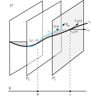
  Figure 6.6: Collapsing dynamical trajectories

Define a one-parameter family of curves $c^{s}:\mathbb{R}\to\mathcal{P}^{\tau}$ by

$$c^{s}(t)=f_{-s}(c_{\phi}(s+t)).$$

By Theorem 6.7(i), $c_{\phi}$ is a dynamical trajectory. Using (6D.4) we see from (6D.5) that each curve $c^{s}$ is also a dynamical trajectory “starting” at $c^{s}(0)=\gamma(s)$.

The tangent to each curve $c^{s}(t)$ at $t=0$ takes the form

$$\left.\frac{d}{dt}c^{s}(t)\right|_{t=0}=X_{0}(\gamma(s))+\zeta_{\mathcal{P}}(\gamma(s)),$$

where $X_{0}$ is a vertical vector field on $\mathcal{P}_{0}$ along $\gamma$. From (6E.13) it follows that $X_{0}(\gamma(s))$ is the tangent to $\gamma$ at $s$.

Proposition 6.6 applied to each dynamical trajectory $c^{s}$ at $t=0$ implies that $X_{0}(\gamma(s))$ satisfies Hamilton’s equations (6E.11) at each point $\gamma(s)$. Since $X_{0}$ is tangent to $\gamma$, Theorem 6.10(ii) shows that the image of $\gamma$ lies in $\mathcal{C}_{0,\zeta}$. In particular, $\gamma(0)=c_{\phi}(0)\in\mathcal{C}_{0,\zeta}$. ∎

This Proposition shows that only initial data $(\varphi,\pi)\in\mathcal{C}_{\lambda,\zeta}$ can be extended to solutions of the Euler–Lagrange equations. The converse is true if we assume well-posedness. We say that the Euler–Lagrange equations are well-posed relative to a slicing $\mathfrak{s}_{Y}$ if every $(\varphi,\pi)\in\mathcal{C}_{\lambda,\zeta}$ can be extended to a dynamical trajectory $c:\,]\lambda-\varepsilon,\lambda+\varepsilon[$ $\subset\mathbb{R}\to\mathcal{P}^{\tau}$ with $c(\lambda)=(\varphi,\pi)$ and that this solution trajectory depends continuously (in a chosen function space topology) on $(\varphi,\pi)$. This will be a standing assumption in what follows.

A4  Well-Posedness

The Euler–Lagrange equations are well-posed.

In this notion of well-posedness, one has to keep in mind that we are assuming that there is a given slicing of the configuration bundle $Y$. However, we will later prove (in Chapter 13) that well-posedness relative to one slicing with a given Cauchy surface $\Sigma$ as a slice will imply well-posedness of any other (appropriate) slicing also containing $\Sigma$ as a slice.

Well-posedness for theories without gauge freedom reduces, in specific examples, to the well-posedness of a system of PDE’s describing that theory in a given slicing. These will be the Hamilton equations that we have developed, written out in coordinates. In the case of metric field theories, one typically would then use theorems on strictly hyperbolic systems to establish well-posedness (relative to a slicing by spacelike hypersurfaces).

The situation for theories with gauge freedom is a bit more subtle. However, it has been established that well-posedness holds for “standard” theories such as Maxwell, Einstein, Yang-Mills and their couplings. Here, very briefly, is how the argument goes for the case of the Einstein equations (in the ADM formulation). To follow this argument, the reader will need to be familiar with works on the initial value formulation of Einstein’s theory, such as Choquet–Bruhat [1962] and Fischer and Marsden [1979b].

If one has a slicing $\mathfrak{s}_{Y}$ specified, and one gives initial data $(\varphi,\pi)\in\mathcal{C}_{0,\zeta}$ over a Cauchy surface $\Sigma_{0}$, then one first takes this data and evolves it using a particular gauge or coordinate choice in which the evolution equations form a strictly hyperbolic (or symmetric hyperbolic) system. This then generates a piece of spacetime on a tubular neighborhood $U$ of the initial hypersurface and the solution $\phi$ so constructed (in this case the metric) on this piece of spacetime varies continuously with the choice of initial data. The solution then satisfies the Euler–Lagrange equation. Since $\Sigma_{0}$ is compact, there exists an $\epsilon>0$ such that $\mathfrak{s}_{X}(]-\epsilon,\epsilon[\times\Sigma)\subset U$. Thus $\phi$ induces the required dynamical trajectory $c_{\phi}:\;]-\epsilon,\epsilon[\;\to\mathcal{P}^{\tau}$ with $c_{\phi}(0)=(\varphi,\pi)$ relative to the given slicing. The argument for other field theories follows a similar pattern.

As was indicated in the Introduction, the above notion of well-posedness is not the same as the question of existence of solutions of the initial value problem for a given choice of lapse and shift (or their generalization, called atlas fields, to other field theories) on a Cauchy surface. This is a more subtle question that we shall address later in Chapter 13. The essential difference is that with a given initial choice of lapse and shift, one still needs to construct the slicing, whereas in the present context we are assuming that a slicing has been given.

There is evidence that well-posedness fails in both of the above senses for many $R+R^{2}$ theories of gravity, as well as for most couplings of higher-spin fields to Einstein’s theory (with supergravity being a notable exception; see Bao, Choquet–Bruhat, Isenberg, and Yasskin [1985]).

This assumption together with Proposition 6.13 yield:

Corollary 6.14.

If A3 and A4 hold, then can_λ(Sol) $=\mathcal{C}_{\lambda,\zeta}$.

Since, as noted previously, ${\rm can}_{\lambda}$ depends only upon the Cauchy surface $\Sigma_{\lambda}$, we have:

Corollary 6.15.

$\mathcal{C}_{\lambda,\zeta}$ is independent of $\zeta$.

Henceforth we denote the final constraint set simply by $\mathcal{C}_{\lambda}$. In particular, this implies that the constraint algorithm computes the same final constraint set regardless of which Hamiltonian $H_{\lambda,\zeta}$ is employed, as the generator $\zeta$ ranges over all compatible slicings (with $\Sigma_{\lambda}$ as a slice).

Proposition 6.13 shows that every dynamical trajectory $c:\mathbb{R}\to\mathcal{P}^{\tau}$ “collapses” to an integral curve of Hamilton’s equations in $\mathcal{C}_{\lambda}$ for each $\lambda$. We now prove the converse; that is, every integral curve of Hamilton’s equations on $\mathcal{C}_{\lambda}$ “suspends” to a dynamical trajectory in $\mathcal{P}^{\tau}$.

Proposition 6.16.

Let $\gamma$ be an integral curve of a tangential solution $X_{\lambda}$ of Hamilton’s equations on $\mathcal{C}_{\lambda}$. Then $c:\mathbb{R}\to\mathcal{P}^{\tau}$ defined by

$$c(s)=f_{s}(\gamma(s))$$ (6E.14)

is a dynamical trajectory.

• Again setting $\lambda=0$, (6E.14) yields

  $$\dot{c}(s)=X_{s}(c(s))+\zeta_{\mathcal{P}}(c(s))$$ (6E.15)

  where $X_{s}=Tf_{s}\cdot X_{0}$. Since $X_{0}(\gamma(s))$ satisfies (6D.7) with $\lambda=0$ for every $s$, (6D.4) implies that $X_{s}(c(s))$ satisfies (6D.7) for every $s$. The desired result now follows from (6E.15) and Proposition 6.6. ∎

Combining the proof of Proposition 6.13 with Proposition 6.16, we have:

Corollary 6.17.

The Euler–Lagrange equations are well-posed iff every tangential solution $X_{\lambda}$ of Hamilton’s equations on $\mathcal{C}_{\lambda}$ integrates to a (local in time) flow for every $\lambda\in\mathbb{R}$.

It remains to discuss the role of gauge transformations in constraint theory. Just as initial value constraints reflect the overdetermined nature of the field equations, gauge transformations arise when these equations are underdetermined.

Classical field theories typically exhibit gauge freedom in the sense that a given set of initial data $(\varphi,\pi)\in\mathcal{C}_{\lambda}$ does not suffice to uniquely determine a dynamical trajectory. Indeed, as noted in Remark 4, if $X_{\lambda}$ is a tangential solution of Hamilton’s equations

$$(X_{\lambda}\mathbin{\hbox to6.0pt{\vrule height=0.4pt,width=5.0pt,depth=0.0pt\kern-0.4pt\vrule height=6.0pt,width=0.4pt,depth=0.0pt\hss}}\,\omega_{\lambda}-\mathbf{d}H_{\lambda,\zeta})\!\bigm{|}\!\mathcal{C}_{\lambda}=0,$$ (6E.16)

then so is $X_{\lambda}+V$ for any vector field $V\in\ker\omega_{\lambda}\cap\mathfrak{X}(\mathcal{C}_{\lambda})$. For this reason we call vectors in $\ker\omega_{\lambda}\cap T\mathcal{C}_{\lambda}$ kinematic directions.

This is not the entire story, however; the indeterminacy in the solutions to the field equations is somewhat more subtle than (6E.16) would suggest. It turns out that solutions of (6E.16) are fixed only up to vector fields in $\mathfrak{X}(\mathcal{C}_{\lambda})\cap\mathfrak{X}(\mathcal{C}_{\lambda})^{\bot}$ which, in general, is larger than $\ker\omega_{\lambda}\cap\mathfrak{X}(\mathcal{C}_{\lambda})$:

$$\ker\omega_{\lambda}\cap\mathfrak{X}(\mathcal{C}_{\lambda})=\mathfrak{X}(\mathcal{P}_{\lambda})^{\bot}\cap\mathfrak{X}(\mathcal{C}_{\lambda})\subset\mathfrak{X}(\mathcal{C}_{\lambda})^{\bot}\cap\mathfrak{X}(\mathcal{C}_{\lambda}).$$

To see this, consider a Hamiltonian vector field $V\in\mathfrak{X}(\mathcal{C}_{\lambda})\cap\mathfrak{X}(\mathcal{C}_{\lambda})^{\bot}$; according to Proposition 6.12(iv), $\mathbf{i}_{V}\omega_{\lambda}=\mathbf{d}f$ where $f$ is a first class constraint. Setting $X^{\prime}_{\lambda}=X_{\lambda}+V$, (6E.16) yields

$$(X^{\prime}_{\lambda}\mathbin{\hbox to6.0pt{\vrule height=0.4pt,width=5.0pt,depth=0.0pt\kern-0.4pt\vrule height=6.0pt,width=0.4pt,depth=0.0pt\hss}}\,\omega_{\lambda}-\mathbf{d}(H_{\lambda,\zeta}+f))\!\bigm{|}\!\mathcal{C}_{\lambda}=0.$$ (6E.17)

Thus if $X_{\lambda}$ is a tangential solution of Hamilton’s equations along $\mathcal{C}_{\lambda}$ with Hamiltonian $H_{\lambda,\zeta}$, then $X^{\prime}_{\lambda}$ is a tangential solution of Hamilton’s equations along $\mathcal{C}_{\lambda}$ with Hamiltonian $H^{\prime}_{\lambda,\zeta}=H_{\lambda,\zeta}+f$.

Physically, equations (6E.16) and (6E.17) are indistinguishable. Put another way, dynamics is insensitive to a modification of the Hamiltonian by the addition of a first class constraint. The reason is that $H^{\prime}_{\lambda,\zeta}=H_{\lambda,\zeta}$ along $\mathcal{C}_{\lambda}$ and it is only what happens along $\mathcal{C}_{\lambda}$ that matters for the physics; distinctions that are only manifested “off” $\mathcal{C}_{\lambda}$—that is, in a dynamically inaccessible region—have no significance whatsoever. Thus the ambiguity in the solutions of Hamilton’s equations is parametrized by $\mathfrak{X}(\mathcal{C}_{\lambda})\cap\mathfrak{X}(\mathcal{C}_{\lambda})^{\bot}$. For further discussion of these points see GNH, Gotay and Nester [1979], and Gotay [1979,​ 1983].

• We may rephrase the content of the last paragraph by saying that what is really of central importance for dynamics is not Hamilton’s equations per se, but rather their pullback to $\mathcal{C}_{\lambda}$; the pullbacks of (6E.16) and (6E.17) to $\mathcal{C}_{\lambda}$ coincide. Furthermore, $\mathfrak{X}(\mathcal{C}_{\lambda})\cap\mathfrak{X}(\mathcal{C}_{\lambda})^{\bot}$ is just the kernel of the pullback of $\omega_{\lambda}$ to $\mathcal{C}_{\lambda}$, cf. (6E.8).

7.

Notice also that since $f$ is first class, (6E.7) and (6E.9) guarantee that the constraint algorithm computes the same final constraint submanifold using either Hamiltonian $H_{\lambda,\zeta}$ or $H^{\prime}_{\lambda,\zeta}$.

8.

The addition of first class constraints to the Hamiltonian (with Lagrange multipliers) is a familiar feature of the Dirac–Bergmann constraint theory.  $\blacklozenge$

The distribution $\mathfrak{X}(\mathcal{C}_{\lambda})\cap\mathfrak{X}(\mathcal{C}_{\lambda})^{\bot}$ on $\mathcal{C}_{\lambda}$ is involutive and so defines a foliation of $\mathcal{C}_{\lambda}$. Initial data $(\varphi,\pi)$ and $(\varphi^{\prime},\pi^{\prime})$ lying on the same leaf of this foliation are said to be gauge-equivalent; solutions obtained by integrating gauge-equivalent initial data cannot be distinguished physically. We call $\mathfrak{X}(\mathcal{C}_{\lambda})\cap\mathfrak{X}(\mathcal{C}_{\lambda})^{\bot}$ the gauge algebra and elements thereof gauge vector fields. The flows of such vector fields preserve this foliation and hence map initial data to gauge-equivalent initial data; they are therefore referred to as gauge transformations.

Proposition 6.12 establishes the fundamental relation between gauge transformations and initial value constraints: first class constraints generate gauge transformations. This encapsulates a curious feature of classical field theory: the field equations being simultaneously overdetermined and underdetermined. These phenomena—a priori quite different and distinct—are intimately correlated via the symplectic structure. Only in special cases (i.e., when $\mathcal{C}_{\lambda}$ is symplectic) can the field equations be overdetermined without being underdetermined. Conversely, it is not possible to have gauge freedom without initial value constraints.

• In Part III we will prove that the Hamiltonian (relative to a $\mathcal{G}$-slicing) of a parametrized field theory in which all fields are variational vanishes on the final constraint set. Pulling (6E.16) back to $\mathcal{C}_{\lambda}$ (cf. Remark 6), it follows that $X_{\lambda}\in{\rm ker}\;\omega_{\mathcal{C}_{\lambda}}$—that is, the evolution is totally gauge! We will explicitly verify this in Examples a, c and d forthwith.  $\blacklozenge$

A more detailed analysis using Proposition 6.12 (see also Chapters 10 and 11) shows that the first class primary constraints correspond to gauge vector fields in $\ker\omega_{\lambda}\cap\mathfrak{X}(\mathcal{C}_{\lambda})$, while first class secondary constraints correspond to the remaining gauge vector fields in $\mathfrak{X}(\mathcal{C}_{\lambda})\cap\mathfrak{X}(\mathcal{C}_{\lambda})^{\bot}$, cf. GNH. In this context, it is worthwhile to mention that second class constraints bear no relation to gauge transformations at all. For if $f$ is second class, then by Proposition 6.12, if it exists its Hamiltonian vector field $X_{\mspace{-1.5mu}f}\in T\mathcal{C}_{\lambda}{}^{\mspace{-1.5mu}\bot}$ everywhere along $\mathcal{C}$, but $X_{\mspace{-1.5mu}f}\notin T\mathcal{C}_{\lambda}$ at least at one point. Thus $X_{\mspace{-1.5mu}f}$ tends to flow initial data off $\mathcal{C}_{\lambda}$, and hence does not generate a transformation of $\mathcal{C}_{\lambda}$. An extensive discussion of second class constraints is given by Lusanna [1991].

The field variables conjugate to the first class primary constraints have a special property which will be important later. We sketch the basic facts here and refer the reader to Part IV for further discussion.

Consider a nonsingular first class primary constraint $f=0$. Let $g$ be canonically conjugate to $f$ in the sense that

$$\omega_{T^{*}\mspace{-1.5mu}\mathcal{Y}_{\lambda}}(X_{\mspace{-1.5mu}f},X_{g})=1.$$

After a canonical change of coordinates, if necessary, we may write

$$\omega_{T^{*}\mspace{-1.5mu}\mathcal{Y}_{\lambda}}=\int_{\Sigma_{\lambda}}[\mathbf{d}g\wedge\mathbf{d}f+\dots]\otimes d^{\mspace{1.5mu}n}\mspace{-1.5mu}x_{0}.$$ (6E.18)

Expressing the evolution vector field $X_{\lambda}$ in the form

$$X_{\lambda}=\frac{dg}{d\lambda}\frac{\delta}{\delta g}+\dots$$

and substituting into Hamilton’s equations (6E.16), we see from (6E.18) that Hamilton’s equations place no restriction on $dg/d\lambda$. Thus, the evolution of $g$ is completely arbitrary; i.e., $g$ is purely “kinematic.” Notice also from (6E.18) that

$$\frac{\delta}{\delta g}=X_{\mspace{-1.5mu}f}\in\ker\omega_{\lambda}\cap\mathfrak{X}(\mathcal{C}_{\lambda}),$$

which shows that ${\delta}/{\delta g}$ is a kinematic direction as defined above.

This concludes our introduction to constraint theory. In Part III we will see how both the initial value constraints and the gauge transformations can be obtained “all at once” from the energy-momentum map for the gauge group.

 

a   Particle Mechanics. We work out the details of the constraint algorithm for the relativistic free particle. Now $\mathcal{P}_{\lambda}\subset T^{*}\mathcal{Y}_{\lambda}$ is defined by the mass constraint (6C.14):

$$\mathfrak{H}=g^{AB}\pi_{A}\pi_{B}+m^{2}=0.$$

Then $\mathfrak{X}(\mathcal{P}_{\lambda})^{\bot}=\ker\omega_{\lambda}$ is spanned by the $\omega_{T^{*}\mspace{-1.5mu}\mathcal{Y}_{\lambda}}$-Hamiltonian vector field

$$X_{\mathfrak{H}}=2g^{AB}\pi_{A}\frac{\partial}{\partial q^{B}}-g^{AB}{}_{,C}\pi_{A}\pi_{B}\frac{\partial}{\partial\pi_{C}}$$ (6E.19)

of the “superhamiltonian” $\mathfrak{H}$. For the Hamiltonian (6C.15), the consistency conditions (6E.4) (cf. (6E.5) with $l=1$) reduce to requiring that $X_{\mathfrak{H}}[H_{\lambda,\zeta}]=0$. A computation gives

$$X_{\mathfrak{H}}[H_{\lambda,\zeta}]=(g^{AB}{}_{,C}\zeta^{C}-2g^{AC}\zeta^{B}{}_{,C})\pi_{A}\pi_{B}=-2\zeta^{(A;B)}\pi_{A}\pi_{B}$$

which vanishes by virtue of the fact that the slicing is Lagrangian, so that $\zeta^{A}\partial/\partial q^{A}$ is a Killing vector field, cf. Example a of §6A. Thus there are no secondary constraints and so $\mathcal{C}_{\lambda}=\mathcal{P}_{\lambda}$. The mass constraint is first class.

The most general evolution vector field satisfying Hamilton’s equations (6E.16) along $\mathcal{P}_{\lambda}$ is $X_{\lambda}=X+kX_{\mathfrak{H}}$, where $X$ is any particular solution and $k\in\mathcal{F}(\mathcal{C}_{\lambda})$ is arbitrary. Explicitly, writing

$$X_{\lambda}=\left(\frac{dq^{A}}{d\lambda}\right)\frac{\partial}{\partial q^{A}}+\left(\frac{d\pi_{A}}{d\lambda}\right)\frac{\partial}{\partial\pi_{A}},$$

the space + time decomposed equations of motion take the form

$$\frac{dq^{A}}{d\lambda} =-\zeta^{A}+2kg^{AB}\pi_{B}$$ (6E.20)

$$\frac{d\pi_{A}}{d\lambda} =\zeta^{B}{}_{,A}\pi_{B}-kg^{BC}{}_{,A}\pi_{B}\pi_{C}.$$

These equations appear complicated because we have written them relative to an arbitrary (but Lagrangian) slicing. If we were to choose the standard slicing $Y=Q\times\mathbb{R}$, then $\zeta^{A}=0$ and (6E.20) are then clearly identifiable as the geodesic equations on $(Q,g)$ with an arbitrary parametrization.

Since the equations of motion (6E.20) for the relativistic free particle are ordinary differential equations, this example is well-posed.

The gauge distribution $\mathfrak{X}(\mathcal{P}_{\lambda})\cap\mathfrak{X}(\mathcal{P}_{\lambda})^{\bot}$ is globally generated by $X_{\mathfrak{H}}$. The gauge freedom of the relativistic free particle is reflected in (6E.20) by the presence of the arbitrary multiplier $k$, and obviously corresponds to time reparametrizations. When $\zeta^{A}=0$ the evolution is purely gauge, as predicted by Remark 9.

b   Electromagnetism. Since $\mathfrak{E}^{0}=0$ is the only primary constraint in Maxwell’s theory, the polar $\mathfrak{X}(\mathcal{P}_{\lambda})^{\bot}$ is spanned by $\delta/\delta A_{0}$. From expression (6C) for the electromagnetic Hamiltonian, we compute that $\delta H_{\lambda,\zeta}/\delta A_{0}=0$ iff

$$\mathfrak{E}^{i}{}_{,i}=0,$$ (6E.21)

where we have performed an integration by parts. This is Gauss’ Law, and defines $\mathcal{P}_{\lambda,\zeta}^{2}\subset\mathcal{P}_{\lambda}$. Continuing with the constraint algorithm, observe that along with ${\delta}/{\delta A_{0}},\ \mathfrak{X}(\mathcal{P}_{\lambda,\zeta}^{2})^{\bot}$ is generated by vector fields of the form $V=(D_{i}f){\delta}/{\delta A_{i}}$, where $f:\mathcal{P}_{\lambda,\zeta}^{2}\rightarrow\mathcal{F}(\Sigma_{\lambda})$ is arbitrary (cf. (5A.6)). But then a computation gives

$$V[H_{\lambda,\zeta}]=-\int_{\Sigma_{\lambda}}\zeta^{j}f_{,j}\mathfrak{E}^{i}{}_{,i}{}{}\,d^{\mspace{1.5mu}3}\mspace{-1.5mu}x_{0}$$

which vanishes by virtue of (6E.21). Thus the algorithm terminates with $\mathcal{C}_{\lambda}=\mathcal{P}_{\lambda,\zeta}^{2}$. Note that $\mathcal{C}_{\lambda}$ is indeed independent of the choice of slicing generator $\zeta$, as promised by Corollary 6.15. Moreover, it is obvious from (6E.21) that $\mathfrak{X}(\mathcal{C}_{\lambda})^{\bot}\subset\mathfrak{X}(\mathcal{C}_{\lambda})$ so $\mathcal{C}_{\lambda}$ is coisotropic and, in fact, all constraints are first class. Note, however, that $H_{\lambda,\zeta}\!\bigm{|}\!\mathcal{C}_{\lambda}\neq 0$ even though this theory is parametrized; the reason is that the metric $g$ is not variational.

Maxwell’s equations in the canonical form (6E.16) are satisfied by the vector field

$$X_{\lambda}=\left(\frac{dA_{0}}{d\lambda}\right)\frac{\delta}{\delta A_{0}}+\left(\frac{dA_{i}}{d\lambda}\right)\frac{\delta}{\delta A_{i}}+\left(\frac{d\mathfrak{E}^{i}}{d\lambda}\right)\frac{\delta}{\delta\mathfrak{E}^{i}}$$

provided

$$\frac{dA_{i}}{d\lambda} =\zeta^{0}N\gamma^{-1/2}\gamma_{ij}\mathfrak{E}^{j}+\frac{1}{N\sqrt{\gamma}}(\zeta^{0}M^{j}+\zeta^{j})\mathfrak{F}_{ji}+(\zeta^{\mu}A_{\mu}-\chi)_{,i}$$ (6E.22)

and

$$\frac{d\mathfrak{E}^{i}}{d\lambda} =\Big{(}\zeta^{0}\gamma^{ik}\gamma^{jm}\mathfrak{F}_{km}+\left[(\zeta^{0}M^{i}+\zeta^{i})\mathfrak{E}^{j}-(\zeta^{0}M^{j}+\zeta^{j})\mathfrak{E}^{i}\right]\Big{)}_{,j}.$$ (6E.23)

Equation (6E.22) reproduces the definition (6C.19) of the electric field density, while (6E.23) captures the dynamical content of Maxwell’s theory. Note that $dA_{0}/d{\lambda}$ is left undetermined, in accord with the fact that ${\delta}/{\delta A_{0}}$ is a kinematic direction.

Since the 4-dimensional form of the Maxwell equations in the Lorentz gauge $A^{\mu}{}_{;\mu}=0$ reduce to wave equations for the $A^{\nu}$ (and hence are hyperbolic), and the gauge itself satisfies the wave equation, this theory is well-posed provided $\Sigma_{\lambda}$ is spacelike. See Misner, Thorne, and Wheeler [1973] and Wald [1984] for details here.

On a Minkowskian background relative to the slicing (6C.24), (6E.22) and (6E.23) take their more familiar forms

$$\frac{dA_{i}}{d\lambda} =\mathfrak{E}_{i}+A_{0,i}-\chi_{,i}$$ (6E.24)

and

$$\frac{d\mathfrak{E}^{i}}{d\lambda} =\mathfrak{F}^{ij}{}_{,j}.$$ (6E.25)

Of course, $X_{\lambda}$ given by (6E.22) and (6E.23) is not uniquely fixed; one can add to it any vector field $V\in\mathfrak{X}(\mathcal{C}_{\lambda})^{\bot}$. Such a $V$ has the form

$$V=f_{0}\frac{\delta}{\delta A_{0}}+D_{i}f\frac{\delta}{\delta A_{i}}$$

for arbitrary maps $f_{0},f:\mathcal{C}_{\lambda}\rightarrow\mathcal{F}(\Sigma_{\lambda})$. The first term in $V$ simply reiterates the fact that the evolution of $A_{0}$ is arbitrary. To understand the significance of the second term in $V$, it is convenient to perform a transverse-longitudinal decomposition of the spatial $1$-form $\mathbb{A}=i_{\lambda}^{*}A$. (For simplicity, we return to the case of a Minkowskian background with the slicing (6C.24).) So split $\mathbb{A}=\mathbb{A}_{T}+\mathbb{A}_{L}$, where $\mathbb{A}_{T}$ is divergence-free and $\mathbb{A}_{L}$ is exact. Then (6E.24) splits into two equations:

$$\frac{d\mathbb{A}_{T}}{d{\lambda}}=\mathfrak{E}\quad\text{ and }\quad\frac{d\mathbb{A}_{L}}{d{\lambda}}=\nabla A_{0}-\nabla\chi.$$

(Note that the electric field is transverse by virtue of (6E.21).) The effect of the second term in $V$ is to thus make the evolution of the longitudinal piece $\mathbb{A}_{L}$ completely arbitrary. In summary, both the temporal and longitudinal components $A_{0}$ and $\mathbb{A}_{L}$ of the potential $A$ are gauge degrees of freedom whose conjugate momenta are constrained to vanish, leaving the transverse part $\mathbb{A}_{T}$ of $A$ and its conjugate momentum $\mathfrak{E}$ as the true dynamical variables of the electromagnetic field.

c   A Topological Field Theory. From (6C.29) we have the instantaneous primary constraint set

$$\mathcal{P}_{\lambda}=\left\{(A,\pi)\in T^{*}{{\mathcal{Y}}}_{\lambda}\mid\pi^{0}=0\>\mbox{ and }\>\pi^{i}=\epsilon^{0ij}A_{j}\right\}.$$

It follows that $\mathfrak{X}(\mathcal{P}_{\lambda})^{\bot}$ is spanned by the vector field ${\delta}/{\delta A^{0}}$. With the Hamiltonian $H_{\lambda,\zeta}$ given by (6C.31), insisting that ${\delta}[H_{\lambda,\zeta}]/{\delta A^{0}}=0$ produces the spatial flatness condition (recall that $n=2$)

$$F_{12}=0.$$ (6E.26)

This equation defines $\mathcal{P}_{\lambda,\zeta}^{2}\subset\mathcal{P}_{\lambda}$. Proceeding, we note that along with ${\delta}/{\delta A_{0}}$, $\mathfrak{X}(\mathcal{P}_{\lambda,\zeta}^{2})^{\bot}$ is generated by vector fields of the form

$$V=D_{i}f\left(\epsilon^{0ij}\frac{\delta}{\delta\pi^{j}}-\frac{\delta}{\delta A_{i}}\right),$$

where $f:\mathcal{P}_{\lambda,\zeta}^{2}\rightarrow\mathcal{F}(\Sigma_{\lambda})$ is arbitrary. But then a computation gives

$$V[H_{\lambda,\zeta}]=\frac{1}{2}\int_{\Sigma_{\lambda}}\epsilon^{0ij}\zeta^{m}f_{,m}F_{ij}\,d^{3}x_{0}$$

which vanishes in view of (6E.26). Thus the constraint algorithm terminates with $\mathcal{C}_{\lambda}=\mathcal{P}_{\lambda,\zeta}^{2}$.

Since $\mathfrak{X}(\mathcal{C}_{\lambda})^{\perp}\subset\mathfrak{X}(\mathcal{C}_{\lambda})$, $\mathcal{C}_{\lambda}$ is coisotropic in $\mathcal{P}_{\lambda}$, whence the secondary constraint (6E.26) is first class. The primary constraint $\pi^{0}=0$ is also first class, while the remaining two primaries $\pi^{i}-\epsilon^{0ij}A_{j}=0$ are second class.

Next, suppose the vector field

$$X_{\lambda}=\left(\frac{dA_{0}}{d\lambda}\right)\frac{\delta}{\delta A_{0}}+\left(\frac{dA_{i}}{d\lambda}\right)\frac{\delta}{\delta A_{i}}+\left(\frac{d\pi^{i}}{d\lambda}\right)\frac{\delta}{\delta\pi^{i}}$$

satisfies the Chern–Simons equations in the Hamiltonian form (6E.16). Then by (6C.30) we must have

$$\frac{dA_{i}}{d\lambda}=(\zeta^{\mu}A_{\mu})_{,i},$$ (6E.27)

and from (6C.28) we then derive

$$\frac{d\pi^{i}}{d\lambda}=\epsilon^{0ij}(\zeta^{\mu}A_{\mu})_{,j}.$$ (6E.28)

As in electromagnetism, ${\delta}/{\delta A_{0}}$ is a kinematic direction with the consequence that $dA_{0}/d{\lambda}$ is left undetermined. By subtracting $dA_{i}/d\lambda$ given by (6E.27) from

$$\dot{A}_{i}=\zeta^{\mu}A_{i,\mu}+A_{\mu}\zeta^{\mu}_{\;\;,i}$$

obtained from (6B.1) while taking (6C.26) into account, we get

$$\zeta^{\mu}(A_{\mu,i}-A_{i,\mu})=0$$

which, when combined with (6E.26), yields the remaining flatness conditions $F_{i0}=0$ in (3C.22). Equation (6E.28) yields nothing new.

Finally, note that (i) when restricted to $\mathcal{C}_{\lambda}$ the Chern–Simons Hamiltonian (6C.31) vanishes by (6E.26), and (ii) we may rearrange

$$X_{\lambda}=\left(\frac{dA_{0}}{d\lambda}\right)\frac{\delta}{\delta A_{0}}-(\zeta^{\mu}A_{\mu})_{,i}\left(\epsilon^{0ij}\frac{\delta}{\delta\pi^{j}}-\frac{\delta}{\delta A_{i}}\right)\in\mathfrak{X}(\mathcal{C}_{\lambda})^{\perp},$$

so that the Chern–Simons evolution is completely gauge, as must be the case for a parametrized field theory in which all fields are variational.

One way to see that the Chern–Simons equations $F_{\mu\nu}=0$ make up a well-posed system is to observe that if we make the gauge choices $A_{0}=0$ and $\zeta_{X}=(1,{\bf 0})$, then the field equations imply that $\partial_{0}A_{\nu}=0$, which clearly determines a unique solution given initial data consisting of $A_{i}$ satisfying $A_{[1,2]}=0$.

d   Bosonic Strings. From (6C.35) and (6C.37) we see that $\mathfrak{X}(\mathcal{P}_{\lambda})^{\bot}$ is spanned by the vector fields ${\delta}/{\delta h_{\sigma\mspace{-1.5mu}\rho}}$ or, equivalently, ${\delta}/{\delta h^{\sigma\mspace{-1.5mu}\rho}}$. Now demand that ${\delta}[H_{\lambda,\zeta}]/{\delta h^{\sigma\mspace{-1.5mu}\rho}}=0$, where $H_{\lambda,\zeta}$ is given by (6C.36). For $(\sigma,\rho)=(1,1)$, this yields

$$\mathfrak{H}=\pi^{2}+\partial\varphi^{2}=0.$$ (6E.29)

Substituting this back into the Hamiltonian and setting $(\sigma,\rho)=(0,1)$, we get

$$\mathfrak{J}=\pi\cdot\partial\varphi=0.$$ (6E.30)

Setting $(\sigma,\rho)=(0,0)$ produces nothing new, so that (6E.29) and (6E.30) are the only secondary constraints. Note that together they imply $H_{\lambda,\zeta}\!\bigm{|}\!\mathcal{P}_{\lambda,\zeta}^{2}=0$, which of course reflects the fact that the bosonic string is a parametrized theory (and also that the slicing is a gauge slicing). As the notation suggests, $\mathfrak{H}$ and $\mathfrak{J}$ are the analogues, for bosonic strings, of the superhamiltonian and supermomentum, respectively, in ADM gravity.

For $N,M\in\mathcal{F}(\Sigma_{\lambda})$, consider the Hamiltonian vector fields

$$X_{N\mspace{-1.5mu}\mathfrak{H}} =2Ng^{AB}\pi_{B}\frac{\delta}{\delta\varphi^{A}}+2g_{AB}\partial(N\partial\varphi^{B})\frac{\delta}{\delta\pi_{A}}$$ (6E.31)

$$X_{M\mathfrak{J}} =M\partial\varphi^{A}\frac{\delta}{\delta\varphi^{A}}+\partial(M\pi_{A})\frac{\delta}{\delta\pi_{A}}$$

of $N\mathfrak{H}$ and $M\mathfrak{J}$, respectively. One verifies that $X_{N\mspace{-1.5mu}\mathfrak{H}}$ and $X_{M\mathfrak{J}}$, together with the ${\delta}/{\delta h_{\sigma\mspace{-1.5mu}\rho}}$, generate $\mathfrak{X}(\mathcal{P}_{\lambda,\zeta}^{2})^{\bot}=\mathfrak{X}(\mathcal{P}_{\lambda,\zeta}^{2})^{\bot}\cap\mathfrak{X}(\mathcal{P}_{\lambda,\zeta}^{2})\subset\mathfrak{X}(\mathcal{P}_{\lambda,\zeta}^{2})$. Since in addition the Hamiltonian vanishes on $\mathcal{P}_{\lambda,\zeta}^{2}$, it follows that the constraint algorithm stops with $\mathcal{P}_{\lambda,\zeta}^{2}=\mathcal{C}_{\lambda}$ and also that all constraints are first class.

Writing the evolution vector field as

$$X_{\lambda}=\left(\frac{d\varphi^{A}}{d\lambda}\right)\frac{\delta}{\delta\varphi^{A}}+\left(\frac{d\pi_{A}}{d\lambda}\right)\frac{\delta}{\delta\pi_{A}}+\left(\frac{dh_{\sigma\mspace{-1.5mu}\rho}}{d\lambda}\right)\frac{\delta}{\delta h_{\sigma\mspace{-1.5mu}\rho}},$$

Hamilton’s equations (6E.16) for the bosonic string are

$$\frac{d\varphi^{A}}{d\lambda} =-2Ng^{AB}\pi_{B}-M\partial\varphi^{A}$$ (6E.32)

$$\frac{d\pi_{A}}{d\lambda} =-2g_{AB}\partial(N\partial\varphi^{B})-\partial(M\pi_{A}).$$ (6E.33)

Here the $dh_{\sigma\mspace{-1.5mu}\rho}/d\lambda$ are undetermined, which is a consequence of the fact that the $h_{\sigma\mspace{-1.5mu}\rho}$ are canonically conjugate to the first class primary constraints $\rho^{\sigma\mspace{-1.5mu}\rho}=0$, and hence are kinematic fields.

Since $X_{\lambda}\in\mathfrak{X}(\mathcal{C}_{\lambda})\cap\mathfrak{X}(\mathcal{C}_{\lambda})^{\bot}$ the evolution is totally gauge. The gauge transformations on the fields $(\varphi^{A},\pi_{A})$ generated by the vector fields $X_{N\mspace{-1.5mu}\mathfrak{H}}$ and $X_{M\mathfrak{J}}$ for $N,M$ arbitrary express the invariance of the bosonic string under diffeomorphisms of $X$ . The complete indeterminacy of the metric $h$ generated by the vector fields ${\delta}/{\delta h_{\sigma\mspace{-1.5mu}\rho}}$ is also a result of invariance under diffeomorphisms—which in two dimensions implies that the conformal factor is the only possible degree of freedom in $h$, cf. §3C.d—coupled with conformal invariance—which implies that even this degree of freedom is gauge. $\blacklozenge$  

In our examples, we have encountered at most secondary constraints, and in Example a there were only primary constraints. This is typical: in mechanics it is rare to find (uncontrived) systems with secondary constraints, and in field theories at most secondary constraints are the rule. (Two exceptional cases are Palatini gravity, which has tertiary constraints (see Part V), and the KdV equation, which has only primary constraints (see Gotay [1988].) In principle, however, the constraint chain (6E.12) can have arbitrary length, but this has no physical significance.

7 The Energy-Momentum Map

In Chapter 4 we defined a covariant momentum mapping for a group $\mathcal{G}$ of covariant canonical transformations of the multisymplectic manifold $Z$. This chapter correlates those ideas with momentum mappings (in the usual sense) on the presymplectic manifold $\mathcal{Z}_{\tau}$ and the symplectic manifold $T^{*}\mathcal{Y}_{\tau}$, and introduces the energy-momentum map on $\mathcal{Z}_{\tau}$. We then show that this energy-momentum map projects to a function $\mathfrak{E}_{\tau}$ on the $\tau$-primary constraint set $\mathcal{P}_{\tau}$, and that under certain circumstances, $\mathfrak{E}_{\tau}$ is identifiable with the negative of the Hamiltonian. This is the key result which enables us in Part III to prove that the final constraint set for first class theories coincides with $\mathfrak{E}^{-1}_{\tau}(0)$, when $\mathcal{G}$ is the gauge group of the theory.

7A Induced Actions on Fields

We first show how group actions on $Y$ and $Z$, etc., can be extended to actions on fields. Given a left action of a group $\mathcal{G}$ on a bundle $\pi_{X\mspace{-1.5mu}K}:K\to X$ covering an action of $\mathcal{G}$ on $X$, we get an induced left action of $\mathcal{G}$ on the space $\mathcal{K}$ of sections of $\pi_{X\mspace{-1.5mu}K}$ defined by

$$\eta_{\mathcal{K}}(\sigma)=\eta_{K}\circ\sigma\circ\eta^{-1}_{X}$$ (7A.1)

for $\eta\in\mathcal{G}$ and $\sigma\in\mathcal{K}$, which generalizes the usual push-forward operation on tensor fields. The infinitesimal generator $\xi_{\mathcal{K}}(\sigma)$ of this action is simply the (negative of the) Lie derivative:

$$\xi_{\mathcal{K}}(\sigma)=-\pounds_{\xi}\sigma=\xi_{K}\circ\sigma-T\sigma\circ\xi_{X}.$$ (7A.2)

We consider the relationship between transformations of the spaces $Z$, $\mathcal{Z}$, and $\mathcal{Z}_{\tau}$. Let $\eta_{Z}:Z\to Z$ be a covariant canonical transformation covering $\eta_{X}:X\to X$ with the induced transformation $\eta_{\mathcal{Z}}:\mathcal{Z}\to\mathcal{Z}$ on fields given by (7A.1). For each $\tau\in{\rm Emb}(\Sigma,X)$, $\eta_{\mathcal{Z}}$ restricts to the mapping

$$\eta_{\mathcal{Z}_{\tau}}:\mathcal{Z}_{\tau}\to\mathcal{Z}_{\eta_{X}\circ\tau}$$

defined by

$$\eta_{\mathcal{Z}_{\tau}}\!(\sigma)=\eta_{Z}\circ\sigma\circ\eta^{-1}_{\tau},$$ (7A.3)

where $\eta_{\tau}:=\eta_{X}\!\bigm{|}\!\Sigma_{\tau}$ is the induced diffeomorphism from $\Sigma_{\tau}$ to $\eta_{X}(\Sigma_{\tau})$.

Proposition 7.1.

$\eta_{\mathcal{Z}_{\tau}}$ is a canonical transformation relative to the two-forms $\Omega_{\tau}$ and $\Omega_{\eta_{X}\circ\tau}$; that is,

$$(\eta_{\mathcal{Z}_{\tau}}\mspace{-1.5mu})^{*}\Omega_{\eta_{X}\circ\tau}=\Omega_{\tau}.$$

• From equation (7A.3)

  $$T\eta_{\mathcal{Z}_{\tau}}\cdot V=T\eta_{Z}\circ(V\circ\eta^{-1}_{\tau})$$ (7A.4)

  for $V\in T_{\sigma}\mathcal{Z}_{\tau}$. Thus,

  $$(\eta_{\mathcal{Z}_{\tau}}\mspace{-1.5mu})^{*} \Omega_{\eta_{X}\circ\tau}(V,W)$$

  $$=\Omega_{\eta_{X}\circ\tau}\left(T\eta_{Z}\cdot V\circ\eta^{-1}_{\tau},T\eta_{Z}\cdot W\circ\eta^{-1}_{\tau}\right)$$ (by (7A.4))

  $$=\int_{\eta_{X}(\Sigma_{\tau})}(\eta_{Z}\circ\sigma\circ\eta^{-1}_{\tau})^{*}(\mathbf{i}_{T\eta_{Z}\cdot W\circ\eta^{-1}_{\tau}}\mathbf{i}_{T\eta_{Z}\cdot V\circ\eta^{-1}_{\tau}}\Omega)$$ (by (5C.3))

  $$=\int_{\eta_{X}(\Sigma_{\tau})}(\eta^{-1}_{\tau})^{*}[\sigma^{*}\eta^{*}_{Z}(\mathbf{i}_{T\eta_{Z}\cdot W}\mathbf{i}_{T\eta_{Z}\cdot V}\Omega)]$$

  $$=\int_{\Sigma_{\tau}}(\sigma^{*}\eta_{Z}{}^{*})(\mathbf{i}_{T\eta_{Z}\cdot W}\mathbf{i}_{T\eta_{Z}\cdot V}\Omega)$$ (change of variables formula)

  $$=\int_{\Sigma_{\tau}}\sigma^{*}(\mathbf{i}_{W}\mathbf{i}_{V}\eta_{Z}{}^{*}\Omega)$$ (by naturality of pull-back)

  $$=\int_{\Sigma_{\tau}}\sigma^{*}(\mathbf{i}_{W}\mathbf{i}_{V}\Omega) \eta$$ (since is covariant canonical)

  $$=\Omega_{\tau}(V,W).$$ (by (5C.3))

  ∎

Similarly, one shows the following:

Proposition 7.2.

If $\eta_{\mathcal{Z}}:\mathcal{Z}\to\mathcal{Z}$ is a special covariant canonical transformation, then $\eta_{\mathcal{Z}_{\tau}}$ is a special canonical transformation.

7B The Energy-Momentum Map

Let $\mathcal{G}$ be a group acting by covariant canonical transformations on $Z$ and let

$$J:Z\to\mathfrak{g}^{*}\otimes\Lambda^{n}Z$$

be a corresponding covariant momentum mapping. This induces the map $E_{\tau}:\mathcal{Z}_{\tau}\to{\mathfrak{g}}^{*}$ defined by

$$\langle E_{\tau}(\sigma),\xi\rangle=\int_{\Sigma_{\tau}}\sigma^{*}\langle J,\xi\rangle$$ (7B.1)

where $\xi\in{\mathfrak{g}}$ and $\langle J,\xi\rangle:Z\to\Lambda^{n}Z$ is defined by $\langle J,\xi\rangle(z):=\langle J(z),\xi\rangle$. While $E_{\tau}$ is not a momentum map in the usual sense on $\mathcal{Z}_{\tau}$—since $\mathcal{G}$ does not necessarily act on $\mathcal{Z}_{\tau}$—it will be shown later to be closely related to the Hamiltonian in the instantaneous formulation of classical field theory. For this reason we shall call $E_{\tau}$ the energy-momentum map. Further justification for this terminology is given in the interlude following this chapter.

For actions on $Z$ lifted from actions on $Y$, using adapted coordinates and (4C.7), (7B.1) becomes

$$\langle E_{\tau}(\sigma),\xi\rangle =\int_{\Sigma_{\tau}}\sigma^{*}\big{(}(p_{A}{}^{\mu}\xi^{A}+p\,\xi^{\mu})\,d^{\mspace{1.5mu}n}\mspace{-1.5mu}x_{\mu}-p_{A}{}^{\mu}\xi^{\nu}dy^{A}\wedge d^{\mspace{1.5mu}n-1}\mspace{-1.5mu}x_{\mu\nu}\big{)}$$

$$=\int_{\Sigma_{\tau}}\big{(}(p_{A}{}^{0}\xi^{A}+p\,\xi^{0})\,d^{\mspace{1.5mu}n}\mspace{-1.5mu}x_{0}-p_{A}{}^{\mu}\xi^{\nu}\sigma^{A}{}_{,i}\,\sigma^{*}(dx^{i}\wedge d^{\mspace{1.5mu}n-1}\mspace{-1.5mu}x_{\mu\nu})\big{)}$$

where the integrands are regarded as functions of $x^{i}$ and where we write, in coordinates, $\sigma(x^{i})=(x^{i},\sigma^{A}(x^{i}),p(x^{i}),p_{A}{}^{\mu}(x^{i}))$. Since

$$dx^{i}\wedge d^{\mspace{1.5mu}n-1}\mspace{-1.5mu}x_{\mu\nu}=\delta^{i}_{\nu}\,d^{\mspace{1.5mu}n}\mspace{-1.5mu}x_{\mu}-\delta^{i}_{\mu}\,d^{\mspace{1.5mu}n}\mspace{-1.5mu}x_{\nu},$$

the expression above can be written in the form

$$\langle E_{\tau}(\sigma),\xi\rangle=\int_{\Sigma_{\tau}}\big{(}p_{A}{}^{0}(\xi^{A}-\xi^{i}\sigma^{A}{}_{,i})+(p+p_{A}{}^{i}\sigma^{A}{}_{,i})\xi^{0}\big{)}\,d^{\mspace{1.5mu}n}\mspace{-1.5mu}x_{0};$$ (7B.2)

that is,

$$\langle E_{\tau}(\sigma),\xi\rangle=\int_{\Sigma_{\tau}}\big{(}p_{A}{}^{0}(\xi^{A}-\xi^{\mu}\sigma^{A}{}_{,\mu})+(p+p_{A}{}^{\mu}\sigma^{A}{}_{,\mu})\xi^{0}\big{)}\,d^{\mspace{1.5mu}n}\mspace{-1.5mu}x_{0},$$ (7B.3)

where (7B.3) is obtained from (7B.2) by adding and subtracting the term $\xi^{0}p_{A}{}^{0}\sigma^{A}{}_{,0}$. (For this to make sense, we suppose that $\sigma$ is the restriction to $\Sigma_{\tau}$ of a section of $\pi_{X\mspace{-1.5mu}Z}$. Of course, (7B.3) is independent of this choice of extension.)

7C Induced Momentum Maps on $\mathcal{Z}_{\tau}$

To obtain a bona fide momentum map on $\mathcal{Z}_{\tau}$, we restrict attention to the subgroup $\mathcal{G}_{\tau}$ of $\mathcal{G}$ consisting of transformations which stabilize the image of $\tau$; that is,

$$\mathcal{G}_{\tau}:=\{\eta\in\mathcal{G}\mid\eta_{X}(\Sigma_{\tau})=\Sigma_{\tau}\}.$$ (7C.1)

We emphasize that the condition $\eta_{X}(\Sigma_{\tau})=\Sigma_{\tau}$ within (7C.1) does not mean that each point of $\Sigma_{\tau}$ is left fixed by $\eta_{X}$, but rather that $\eta_{X}$ moves the whole Cauchy surface $\Sigma_{\tau}$ onto itself.

For any $\eta\in\mathcal{G}_{\tau}$, the map $\eta_{\tau}:=\eta_{X}\!\bigm{|}\!\Sigma_{\tau}$ is an element of $\operatorname{Diff}(\Sigma_{\tau})$. It follows from Proposition 7.1 that

$$\eta_{\mathcal{Z}_{\tau}}\!(\sigma)=\eta_{Z}\circ\sigma\circ\eta^{-1}_{\tau}$$ (7C.2)

is a canonical action of $\mathcal{G}_{\tau}$ on $\mathcal{Z}_{\tau}$. From (7A.2), the infinitesimal generator of this action is

$$\xi_{\mathcal{Z}_{\tau}}\!(\sigma)=\xi_{Z}\circ\sigma-T\sigma\circ\xi_{\tau},$$ (7C.3)

where $\xi_{\tau}$ generates $\eta_{\tau}$.

Being a subgroup of $\mathcal{G}$, $\mathcal{G}_{\tau}$ has a covariant momentum map which is given by $J$ followed by the projection from ${\mathfrak{g}}^{*}\otimes\Lambda^{n}Z$ to ${\mathfrak{g}}^{*}_{\tau}\otimes\Lambda^{n}Z$, where ${\mathfrak{g}}_{\tau}$ is the Lie algebra of $\mathcal{G}_{\tau}$. Note that in adapted coordinates, $\xi\in{\mathfrak{g}}_{\tau}$ when $\xi_{X}^{0}=0$ on $\Sigma_{\tau}$. From (7B.1), the map $J$ induces the map $J_{\tau}:=E_{\tau}\!\bigm{|}{\mathfrak{g}}_{\tau}:\mathcal{Z}_{\tau}\to{\mathfrak{g}}^{*}_{\tau}$ given by

$$\langle J_{\tau}(\sigma),\xi\rangle=\int_{\Sigma_{\tau}}\sigma^{*}\langle J,\xi\rangle$$ (7C.4)

for $\xi\in{\mathfrak{g}}_{\tau}$.

Proposition 7.3.

$J_{\tau}$ is a momentum map for the $\mathcal{G}_{\tau}$-action on $\mathcal{Z}_{\tau}$ defined by (7C.2), and it is $\operatorname{Ad}^{*}$-equivariant if $J$ is.

• Let $V\in T_{\sigma}\mathcal{Z}_{\tau}$ and let $v$ be a $\pi_{XZ}$-vertical vector field on $Z$ such that $V=v\circ\sigma$. If $f_{\lambda}$ is the flow of $v$, let $\sigma_{\lambda}=f_{\lambda}\circ\sigma$ so that the curve $\sigma_{\lambda}\in\mathcal{Z}_{\tau}$ has tangent vector $V$ at $\lambda=0$. Therefore, with $J_{\tau}$ defined by (7C.4),we have

  $$\langle\mathbf{i}_{V}\mathbf{d}J_{\tau}(\sigma),\xi\rangle=\frac{d}{d\lambda}\left.\left[\int_{\Sigma_{\tau}}\sigma^{*}_{\lambda}\langle J,\xi\rangle\right]\right|_{\lambda=0}=\int_{\Sigma_{\tau}}\sigma^{*}\text{\pounds}_{v}\langle J,\xi\rangle.$$

  But

  $$\int_{\Sigma_{\tau}}\sigma^{*}\pounds_{v}\langle J,\xi\rangle=\int_{\Sigma_{\tau}}\sigma^{*}(\mathbf{d}\mspace{1.5mu}\mathbf{i}_{v}\langle J,\xi\rangle+\mathbf{i}_{v}\mathbf{d}\langle J,\xi\rangle),$$

  and since $\Sigma$ is compact and boundaryless,

  $$\int_{\Sigma_{\tau}}\sigma^{*}(\mathbf{d}\mspace{1.5mu}\mathbf{i}_{v}\langle J,\xi\rangle)=\int_{\Sigma_{\tau}}\mathbf{d}\sigma^{*}(\mathbf{i}_{v}\langle J,\xi\rangle)=0$$

  by Stokes’ theorem. Therefore, by the definition (4C.3) of a covariant momentum mapping,

  $$\langle\mathbf{i}_{V}\mathbf{d}J_{\tau}(\sigma),\xi\rangle=\int_{\Sigma_{\tau}}\sigma^{*}(\mathbf{i}_{v}\mathbf{d}\langle J,\xi\rangle)=\int_{\Sigma_{\tau}}\sigma^{*}[\mathbf{i}_{v}\mathbf{i}_{\xi_{Z}}\Omega].$$ (7C.5)

  Note that $\xi_{Z}$ need not be $\pi_{X\mspace{-1.5mu}Z}$-vertical, so we cannot yet use Lemma 5.1.

  Now for any $w\in T\Sigma_{\tau}$, we have

  $$\sigma^{*}(\mathbf{i}_{v}\mathbf{i}_{T\sigma\cdot w}\Omega)=-\sigma^{*}(\mathbf{i}_{T\sigma\cdot w}\mathbf{i}_{v}\Omega)=-\mathbf{i}_{W}\sigma^{*}(\mathbf{i}_{v}\Omega)=0$$

  by the naturality of pull-back and the fact that $\sigma^{*}(\mathbf{i}_{v}\Omega)$ vanishes since it is an $(n+1)$-form on an $n$-manifold. In particular, for $w=\xi_{\tau}$, we have

  $$\sigma^{*}(\mathbf{i}_{v}\mathbf{i}_{T\sigma\cdot\xi_{\tau}}\Omega)=0.$$

  Combining this result with (7C.5) and using the fact that $\xi_{Z}-T\sigma\cdot\xi_{\tau}$ is $\pi_{X\mspace{-1.5mu}Z}$-vertical, we get

  $$\langle\mathbf{i}_{V}\mathbf{d}J_{\tau}(\sigma),\xi\rangle =\int_{\Sigma_{\tau}}\sigma^{*}(\mathbf{i}_{v}\mathbf{i}_{\xi_{Z}-T\sigma\cdot\xi_{\tau}}\Omega)$$

  $$=\Omega_{\tau}(\xi_{\mathcal{Z}_{\tau}},V)$$

  by (7C.3) and (5C.3). Thus $J_{\tau}$ is a momentum map.

  To show that $J_{\tau}$ is Ad^∗-equivariant, we verify that for $\eta\in\mathcal{G}_{\tau}$ and $\xi\in{\mathfrak{g}}_{\tau}$, $J_{\tau}$ satisfies the condition

  $$\langle J_{\tau}(\sigma),{\rm Ad}_{\eta^{-1}}\xi\rangle=\langle J_{\tau}(\eta_{\mathcal{Z}_{\tau}}\!(\sigma)),\xi\rangle.$$

  However, from (7C.4) and (4C.4), we have

  $$\langle J_{\tau}(\sigma),{\rm Ad}_{\eta^{-1}}\xi\rangle=\int_{\Sigma_{\tau}}\sigma^{\ast}\langle J,{\rm Ad}_{\eta^{-1}}\xi\rangle=\int_{\Sigma_{\tau}}\sigma^{\ast}\eta_{Z}{}^{\ast}\langle J,\xi\rangle;$$

  whereas from (7C.2), (7C.4), and the change of variables formula, we get

  $$\langle J_{\tau}(\eta_{\mathcal{Z}_{\tau}}\!(\sigma)),\xi\rangle =\int_{\Sigma_{\tau}}(\eta_{Z}\circ\sigma\circ\eta^{-1}_{\tau})^{*}\langle J,\xi\rangle$$

  $$=\int_{\Sigma_{\tau}}(\eta^{-1}_{\tau})^{*}\sigma^{*}\eta_{Z}{}^{*}\langle J,\xi\rangle$$

  $$=\int_{\Sigma_{\tau}}\sigma^{*}\eta_{Z}{}^{*}\langle J,\xi\rangle,$$

  thereby establishing the desired equality. ∎

7D Induced Momentum Maps on $T^{*}\mathcal{Y}_{\tau}$

We now demonstrate how the group actions and momentum maps carry over from the multisymplectic context to the instantaneous formalism. Recall that the phase space $(T^{*}\mathcal{Y}_{\tau},\omega_{\tau})$ is the symplectic quotient of the presymplectic manifold $(\mathcal{Z}_{\tau},\Omega_{\tau})$ by the map $R_{\tau}$. The key observation is that both the action of $\mathcal{G}_{\tau}$ and the momentum map $J_{\tau}$ pass to the quotient.

First consider a canonical transformation $\eta_{\mathcal{Z}_{\tau}}:\mathcal{Z}_{\tau}\to\mathcal{Z}_{\tau}$. Define a map $\eta_{T^{*}\mspace{-1.5mu}\mathcal{Y}_{\tau}}:T^{*}\mathcal{Y}_{\tau}\to T^{*}\mathcal{Y}_{\tau}$ as follows: For each $\pi\in T^{*}_{\varphi}\mathcal{Y}_{\tau}$, set

$$\eta_{T^{*}\mspace{-1.5mu}\mathcal{Y}_{\tau}}\!(\pi)=R_{\tau}(\eta_{\mathcal{Z}_{\tau}}\!(\sigma))$$ (7D.1)

where $\sigma$ is any element of $R^{-1}_{\tau}(\{\pi\})$.

Proposition 7.4.

The map $\eta_{T^{*}\mspace{-1.5mu}\mathcal{Y}_{\tau}}$ is a canonical transformation.

• To begin, we must show that $\eta_{T^{*}\mspace{-1.5mu}\mathcal{Y}_{\tau}}$ is well-defined; that is

  $$R_{\tau}(\eta_{\mathcal{Z}_{\tau}}\!(\sigma))=R_{\tau}(\eta_{\mathcal{Z}_{\tau}}\!(\sigma^{\prime}))\quad\text{ whenever }\quad\sigma,\sigma^{\prime}\in R^{-1}_{\tau}(\{\pi\}).$$

  Since $\eta_{\mathcal{Z}_{\tau}}$ is a canonical transformation, it preserves the kernel of $\Omega_{\tau}$. But this kernel equals the kernel of $TR_{\tau}$ by Corollary 5.3(ii). Therefore, $\eta_{\mathcal{Z}_{\tau}}$ preserves the fibers of $R_{\tau}$, and so $\eta_{T^{*}\mspace{-1.5mu}\mathcal{Y}_{\tau}}$ is well defined.

  Since $\eta_{\mathcal{Z}_{\tau}}$ is a diffeomorphism and $R_{\tau}$ is a submersion, $\eta_{T^{*}\mspace{-1.5mu}\mathcal{Y}_{\tau}}$ is a diffeomorphism. That the map $\eta_{T^{*}\mspace{-1.5mu}\mathcal{Y}_{\tau}}$ preserves the symplectic form $\omega_{\tau}$ is a straightforward computation using (7D.1), Corollary 5.3, and the definitions. ∎

This Proposition shows that the canonical action of $\mathcal{G}_{\tau}$ on $\mathcal{Z}_{\tau}$ gives rise to a canonical action of $\mathcal{G}_{\tau}$ on $T^{*}\mathcal{Y}_{\tau}$ such that $R_{\tau}$ is equivariant; that is, for $\eta\in\mathcal{G}_{\tau}$, the following diagram commutes:

$$\begin{CD}\mathcal{Z}_{\tau}@>{R_{\tau}}>{}>T^{*}\mathcal{Y}_{\tau}\\ @V{\eta_{\mathcal{Z}_{\tau}}}V{}V@V{}V{\eta_{T^{*}\mspace{-1.5mu}\mathcal{Y}_{\tau}}}V\\ \mathcal{Z}_{\tau}@>{}>{R_{\tau}}>T^{*}\mathcal{Y}_{\tau}\end{CD}$$

Regarding momentum maps, we have:

Proposition 7.5.

If $J_{\tau}$ is a momentum map for the action of $\mathcal{G}_{\tau}$ on $\mathcal{Z}_{\tau}$, then $\mathcal{J}_{\tau}:T^{*}\mathcal{Y}_{\tau}\to{\mathfrak{g}}^{*}_{\tau}$ defined by the diagram

(7D.2)

is a momentum map for the induced action of $\mathcal{G}_{\tau}$ on $T^{*}\mathcal{Y}_{\tau}$. Further, if $J_{\tau}$ is Ad^∗-equivariant, then so is $\mathcal{J}_{\tau}$.

• This is a consequence of the facts that $R_{\tau}$ is equivariant and $R_{\tau}{}^{*}\omega_{\tau}=\Omega_{\tau}$. ∎

We emphasize that the momentum map $\mathcal{J}_{\tau}$, which we have defined on $T^{*}\mathcal{Y}_{\tau}$, corresponds to the action of $\mathcal{G}_{\tau}$ only. For the full group $\mathcal{G}$, the corresponding energy-momentum map does not pass from $\mathcal{Z}_{\tau}$ to $T^{*}\mathcal{Y}_{\tau}$. However, as we will see in §7F, the energy-momentum map $E_{\tau}$ does project to the primary constraint submanifold in $T^{*}\mathcal{Y}_{\tau}$.

7E Momentum Maps for Lifted Actions

For lifted actions we are able to obtain explicit formulas for the energy-momentum and momentum maps on $\mathcal{Z}_{\tau}$ and $T^{*}\mathcal{Y}_{\tau}$ and the relationship between them. Suppose the action of $\mathcal{G}$ on $Z$ is obtained by lifting an action of $\mathcal{G}$ on $Y$. Then $\eta\in\mathcal{G}$ maps $\mathcal{Y}_{\tau}$ to $\mathcal{Y}_{\eta_{X}\circ\tau}$ according to

$$\eta_{\mathcal{Y}_{\tau}}\!(\varphi)=\eta_{Y}\circ\varphi\circ\eta^{-1}_{\tau}$$ (7E.1)

where $\eta_{\tau}=\eta_{X}\!\bigm{|}\!\Sigma_{\tau}$. This in turn restricts to an action of $\mathcal{G}_{\tau}$ on $\mathcal{Y}_{\tau}$ given by the same formula, with the infinitesimal generator

$$\xi_{\mathcal{Y}_{\tau}}\!(\varphi)=\xi_{Y}\circ\varphi-T\varphi\circ\xi_{\tau}$$ (7E.2)

where $\xi_{\tau}=\xi_{X}\!\bigm{|}\!\Sigma_{\tau}$.

Corollary 7.6.

For actions lifted from $Y$:

1. The energy-momentum map on $\mathcal{Z}_{\tau}$ is

   $$\langle E_{\tau}(\sigma),\xi\rangle=\int_{\Sigma_{\tau}}\varphi^{*}(\mathbf{i}_{\xi_{Y}}\sigma)$$ (7E.3)

   where $\xi\in{\mathfrak{g}}$, and $\varphi=\pi_{Y\!Z}\circ\sigma$.

2. The induced $\mathcal{G}_{\tau}$-action on $T^{*}\mathcal{Y}_{\tau}$ given by (7D.1) is the usual cotangent action; that is,

   $$\eta_{T^{*}\mspace{-1.5mu}\mathcal{Y}_{\tau}}\!(\pi)=(\eta^{-1}_{\mathcal{Y}_{\tau}})^{*}\pi.$$

3. The corresponding induced momentum map $\mathcal{J}_{\tau}$ on $T^{*}\mathcal{Y}_{\tau}$ defined by (7D.2) is the standard one; that is,

   $$\langle\mathcal{J}_{\tau}(\varphi,\pi),\xi\rangle=\langle\pi,\xi_{\mathcal{Y}_{\tau}}\!(\varphi)\rangle=\int_{\Sigma_{\tau}}\pi\left(\xi_{\mathcal{Y}_{\tau}}\!(\varphi)\right)$$ (7E.4)

   for $\xi\in{\mathfrak{g}}_{\tau}$. Moreover, the momentum maps $J,J_{\tau}$, and $\mathcal{J}_{\tau}$ are all Ad^∗-equivariant.

• To prove (i), substitute formula (4C.6) into (7B.1) and note that

  $$\sigma^{*}\langle J,\xi\rangle=\sigma^{*}\pi_{Y\!Z}{}^{*}\mathbf{i}_{\xi_{Y}}\sigma=\varphi^{*}\mathbf{i}_{\xi_{Y}}\sigma.$$ (7E.5)

  To prove (ii) let $\eta\in\mathcal{G}_{\tau}$, $\pi=R_{\tau}(\sigma)\in T^{*}_{\varphi}\mathcal{Y}_{\tau}$ and $V\in T_{\eta_{\mathcal{Y}_{\tau}}\mspace{-1.5mu}(\varphi)}\mathcal{Y}_{\tau}$. Then

  $$\langle\eta_{T^{*}\!\mathcal{Y}_{\tau}}\mspace{-1.5mu}(\pi),V\rangle$$

  $$\quad=\langle R_{\tau}(\eta_{\mathcal{Z}_{\tau}}\!(\sigma)),V\rangle$$ (by (7D.1))

  $$\quad=\int_{\Sigma_{\tau}}(\eta_{\mathcal{Y}_{\tau}}\!(\varphi))^{*}[\mathbf{i}_{V}(\eta_{\mathcal{Z}_{\tau}}\!(\sigma))]$$ (by (5D.1))

  $$\quad=\int_{\Sigma_{\tau}}(\eta^{-1}_{\tau})^{*}\varphi^{*}\eta_{Y}{}^{*}[\mathbf{i}_{V}(\eta_{\mathcal{Z}_{\tau}}\!(\sigma))]$$ (by (7E.1))

  $$\quad=\int_{\Sigma_{\tau}}\varphi^{*}\eta_{Y}{}^{*}[\mathbf{i}_{V}(\eta_{\mathcal{Z}_{\tau}}\!(\sigma))]$$ (by the change of variables formula)

  $$\quad=\int_{\Sigma_{\tau}}\varphi^{*}[\mathbf{i}_{T\eta^{-1}_{Y}\cdot V}\eta_{Y}{}^{*}(\eta_{\mathcal{Z}_{\tau}}\!(\sigma))]$$

  $$\quad=\int_{\Sigma_{\tau}}\varphi^{*}[\mathbf{i}_{T\eta^{-1}_{Y}\cdot V}\sigma]$$ (by (4B.3))

  $$\quad=\langle R_{\tau}(\sigma),{T\eta^{-1}_{Y}\cdot V}\rangle$$ (by (5D.1))

  $$\quad=\langle\pi,{T\eta^{-1}_{Y}\cdot V}\rangle$$

  $$\quad=\langle(\eta^{-1}_{Y})^{*}\pi,V\rangle.$$

  To prove (iii) we compute, taking into account (7D.2), (7E.3), and (7E.2),

  $$\langle\mathcal{J}_{\tau}(R_{\tau}(\sigma)),\xi\rangle =\langle J_{\tau}(\sigma),\xi\rangle=\int_{\Sigma_{\tau}}\varphi^{*}(\mathbf{i}_{\xi_{Y}}\sigma)$$

  $$=\int_{\Sigma_{\tau}}\varphi^{*}(\mathbf{i}_{\xi_{Y}-T\varphi\cdot\xi_{\tau}}\sigma)=\langle R_{\tau}(\sigma),\xi_{\mathcal{Y}_{\tau}}\!(\varphi)\rangle,$$

  where we have used

  $$\varphi^{*}\mathbf{i}_{T\varphi\cdot\xi_{\tau}}\sigma=\mathbf{i}_{\xi_{\tau}}\varphi^{*}\sigma=0$$

  since $\varphi^{*}\sigma$ is an $(n+1)$-form on the $n$-manifold $\Sigma_{\tau}$.

  Finally, equivariance follows from Propositions 4.3, 7.3 and 7.5. ∎

7F The Hamiltonian and the Energy-Momentum Map

In §7B we defined the energy-momentum map $E_{\tau}$ on $\mathcal{Z}_{\tau}$. Here we show that for lifted actions, $E_{\tau}$ projects to a well-defined function

$$\mathcal{E}_{\tau}:\mathcal{P}_{\tau}\to{\mathfrak{g}}^{*}$$

on the $\tau$-primary constraint set, which we refer to as the “instantaneous energy-momentum map.” This is the central object for our later analysis.

Let the group $\mathcal{G}$ act on $Y$ and consider the lifted action of $\mathcal{G}$ on $Z$. Using (4C.5) rewrite formula (7B.1) as

$$\langle E_{\tau}(\sigma),\xi\rangle=\int_{\Sigma_{\tau}}\langle\mathfrak{E}_{\tau}(\sigma),\xi\rangle$$

for $\sigma\in\mathcal{Z}_{\tau}$ and $\xi\in{\mathfrak{g}}$, where

$$\langle\mathfrak{E}_{\tau}(\sigma),\xi\rangle=\sigma^{*}(\mathbf{i}_{\xi_{Z}}\Theta)$$ (7F.1)

defines the energy-momentum density $\mathfrak{E}_{\tau}$.

While $\mathfrak{E}_{\tau}$ does not directly factor through the reduction map to give an instantaneous energy-momentum density on $T^{*}\mathcal{Y}_{\tau}$, we nonetheless have:

Proposition 7.7.

The energy-momentum density $\mathfrak{E}_{\tau}$ induces an instantaneous energy-momentum density on $\mathcal{P}_{\tau}\subset T^{*}\mathcal{Y}_{\tau}$.

• Given any $(\varphi,\pi)\in\mathcal{P}_{\tau}$, let $\sigma$ be a holonomic lift of $(\varphi,\pi)$ to $\mathcal{N}_{\tau}$ (cf. §6C). We claim that for any $x\in\Sigma_{\tau}$ and $\xi\in\mathfrak{g}$, the quantity

  $$\langle\mathfrak{E}_{\tau}(\sigma)(x),\xi\rangle\in\Lambda^{n}_{x}\Sigma_{\tau}$$

  depends only upon $j^{1}\mspace{-1.5mu}\varphi(x)$ and $\pi(x)$. Thus, setting

  $$\langle\mathfrak{E}_{\tau}(\varphi,\pi)(x),\xi\rangle=\langle\mathfrak{E}_{\tau}(\sigma)(x),\xi\rangle$$ (7F.2)

  defines the instantaneous energy-momentum density (which we denote by the same symbol $\mathfrak{E}_{\tau}$) on $\mathcal{P}_{\tau}$.

If $\xi_{X}(x)$ is transverse to $\Sigma_{\tau}$, then (7F.1) combined with (6C.10) gives

$$\langle\mathfrak{E}_{\tau}(\sigma)(x),\xi\rangle=-\mathfrak{H}_{\tau,\xi}(\varphi,\pi)(x).$$ (7F.3)

On the other hand, if $\xi_{X}(x)\in T_{x}\Sigma_{\tau}$, then from (7E.5) we compute

$$\langle\mathfrak{E}_{\tau}(\sigma)(x),\xi\rangle=\varphi^{*}(\mathbf{i}_{\xi_{Y}(\varphi(x))}\sigma(x))=\varphi^{*}(\mathbf{i}_{\xi_{Y}(\varphi(x))-T_{x}\varphi\cdot\xi_{X}(x)}\sigma(x))$$ (7F.4)

where we have used the same ‘trick’ as in the proof of Corollary 7.6(iii). Since $\xi_{Y}-T\varphi\cdot\xi_{X}$ is $\pi_{XY}$-vertical, we can now apply (5D.2) to obtain

$$\langle\mathfrak{E}_{\tau}(\sigma)(x),\xi\rangle =\big{\langle}R_{\tau}(\sigma)(x),{\xi_{Y}(\varphi(x))-T_{x}\varphi\cdot\xi_{X}(x)}\big{\rangle}$$

$$=\langle\pi(x),\xi_{\mathcal{Y}_{\tau}}\!(\varphi)(x)\rangle.$$ (7F.5)

In either case, $\langle\mathfrak{E}_{\tau}(\sigma)(x),\xi\rangle$ depends only upon the values of $\varphi$, its first derivatives, and $\pi$ along $\Sigma_{\tau}$. Thus the definition (7F.2) is meaningful for any $\xi\in{\mathfrak{g}}$. ∎

Integrating (7F.2), we get the instantaneous energy-momentum map $\mathcal{E}_{\tau}:\mathcal{P}_{\tau}\to{\mathfrak{g}}^{*}$ defined by

$$\langle\mathcal{E}_{\tau}(\sigma),\xi\rangle=\int_{\Sigma_{\tau}}\langle\mathfrak{E}_{\tau}(\varphi,\pi),\xi\rangle.$$ (7F.6)

Two cases warrant special attention:

Corollary 7.8.

Let $\xi\in{\mathfrak{g}}$.

1. If $\xi_{X}$ is everywhere transverse to $\Sigma_{\tau}$, then

   $$\langle\mathcal{E}_{\tau}(\varphi,\pi),\xi\rangle=-H_{\tau,\xi}(\varphi,\pi)$$ (7F.7)

2. If $\xi_{X}$ is everywhere tangent to $\Sigma_{\tau}$, then

   $$\langle\mathcal{E}_{\tau}(\varphi,\pi),\xi\rangle=\langle\mathcal{J}_{\tau}(\varphi,\pi),\xi\rangle.$$ (7F.8)

• Assertion (i) follows from (7F.3) and (ii) is a consequence of (7F) and (7E.4). ∎

• In general, $\mathcal{E}_{\tau}$ is defined only on the primary constraint set $\mathcal{P}_{\tau}$, as $H_{\tau,\xi}$ is. However, if $\mathcal{G}=\mathcal{G}_{\tau}$, then $\mathcal{E}_{\tau}=\mathcal{J}_{\tau}$ is defined on all of $T^{*}\mathcal{Y}_{\tau}$. (It was not necessary that $\sigma$ be a holonomic lift for the proof of the second part of Proposition 7.7, corresponding to the case when $\xi_{X}(x)\in T_{x}\Sigma_{\tau}.$)

2.

Although the instantaneous energy-momentum map can be identified with the Hamiltonian (when $\xi_{X}\pitchfork\Sigma_{\tau}$) and the momentum map $\mathcal{J}_{\tau}$ for $\mathcal{G}_{\tau}$ (when $\xi_{X}\,\|\>\Sigma_{\tau})$, it is important to realize that $\langle\mathcal{E}_{\tau}(\varphi,\pi),\xi\rangle$ is defined for any $\xi\in{\mathfrak{g}}$, regardless of whether or not it is everywhere transverse or tangent to $\Sigma_{\tau}$.

3.

The relation (7F.7) between the instantaneous energy-momentum map and the Hamiltonian is only asserted to be valid in the context of lifted actions; for more general actions, we do not claim such a relationship. Fortunately, in most examples, lifted actions are the appropriate ones to consider.  $\blacklozenge$

The instantaneous energy-momentum map $\mathcal{E}_{\tau}$ on $\mathcal{P}_{\tau}$ is the cornerstone of our work since, via (7F.7) above, it constitutes the fundamental link between dynamics and the gauge group. From it we will be able to correlate the notion of “gauge transformation” as arising from the gauge group action with that in the Dirac–Bergmann theory of constraints. This in turn will make it possible to “recover” the first class initial value constraints from $\mathcal{E}_{\tau}$ because, according to §6E, they are the generators of gauge transformations.

• Indeed, in Chapter 11 we will show that for parametrized theories in which all fields are variational, the final constraint set $\mathcal{C}_{\tau}\subset\mathcal{E}_{\tau}^{-1}(0).$ Combining this with the relation (7F.7), we see that for such theories the Hamiltonian (defined relative to a $\mathcal{G}$-slicing) must vanish “on shell;” that is, $H_{\tau,\xi}\!\bigm{|}\!\mathcal{C}_{\tau}=0$ as predicted in Remark 9 in §6E.  $\blacklozenge$

Thus, in some sense, the energy-momentum map encodes in a single geometric object virtually all of the physically relevant information about a given classical field theory: its dynamics, its initial value constraints and its gauge freedom. Momentarily, in Interlude II, we will see that $\mathcal{E}_{\tau}$ also incorporates the stress-energy-momentum tensor of a theory. It is these properties of $\mathcal{E}_{\tau}$ that will eventually enable us to achieve our main goal; viz., to write the evolution equations in adjoint form.

 

a   Particle Mechanics. If $\mathcal{G}=\operatorname{Diff}(\mathbb{R})$ acts on $Y=\mathbb{R}\times Q$ by time reparametrizations, then from (4C.9) the energy-momentum map on $\mathcal{Z}_{t}=\mathbb{R}\times T^{*}Q$ is

$$\langle E_{t}(p,q^{1},\cdots,q^{N},p_{1},\cdots,p_{N}),\chi\rangle=p\chi(t).$$

But $p=0$ on $\mathcal{N}$ by virtue of the time reparametrization-invariance of $\mathcal{L}$, cf. example a in §4D. Thus the instantaneous energy momentum map on $\mathcal{P}_{t}=R_{t}(\mathcal{N}_{t})$ vanishes. The subgroup $\mathcal{G}_{t}$ consists of those diffeomorphisms which fix $\tau(\Sigma)=t\in\mathbb{R}$. However, the actions of $\mathcal{G}_{t}$ on $\mathcal{Z}_{t}$ and on $T^{*}\mathcal{Y}_{t}=T^{*}Q$ are trivial.

If $\mathcal{G}={\rm Diff}(\mathbb{R})\times G$, where $G$ acts only on the factor $Q$, then $\mathcal{G}_{t}=G$. In this case, $\mathcal{J}_{t}$ reduces to the usual momentum map on $T^{*}Q$.

b   Electromagnetism. For electromagnetism on a fixed background with $\mathcal{G}=\mathcal{F}(X)$, we find from (4C.12) and (7B.1) that in adapted coordinates,

$$\langle E_{\tau}(A,p,\mathfrak{F}),\chi\rangle=\int_{\Sigma_{\tau}}\mathfrak{F}^{\nu 0}\chi{}_{,\nu}\,d^{\mspace{1.5mu}3}\mspace{-1.5mu}x_{0}$$

for $\chi\in\mathcal{F}(X)$. Now $\mathcal{G}=\mathcal{G}_{\tau}$, so in this case $\mathcal{J}_{\tau}$ and $\mathcal{E}_{\tau}$ coincide. Using the expression above for $E_{\tau}$, (7D.2), and $\mathfrak{E}^{\nu}=\mathfrak{F}^{\nu 0}$, we get

$$\langle\mathcal{J}_{\tau}(A,\mathfrak{E}),\chi\rangle=\int_{\Sigma_{\tau}}\mathfrak{E}^{\nu}\chi{}_{,\nu}\,d^{\mspace{1.5mu}3}\mspace{-1.5mu}x_{0}$$ (7F.9)

on $T^{*}\mathcal{Y}_{\tau}$. Note that this agrees with formula (7E.4). When restricted to the primary constraint set $\mathcal{P}_{\tau}\subset T^{*}\mathcal{Y}_{\tau}$ given by $\mathfrak{E}^{0}=0$, (7F.9) becomes

$$\langle\mathcal{E}_{\tau}(A,\mathfrak{E}),\chi\rangle=\int_{\Sigma_{\tau}}\mathfrak{E}^{i}\chi{}_{,i}\,d^{\mspace{1.5mu}3}\mspace{-1.5mu}x_{0}.$$ (7F.10)

In the parametrized case, when $\mathcal{G}={\rm Diff}(X)\;\circledS\;\mathcal{F}(X)$, $E_{\tau}$ is replaced by $\tilde{E}_{\tau}$ where, with the help of (4C.17),

$$\langle{\tilde{E}_{\tau}}(A, \,p,\mathfrak{F};g),(\xi,\chi)\rangle$$

$$=\int_{\Sigma_{\tau}}\big{(}{\mathfrak{F}}^{\nu 0}(-A_{\mu}\xi^{\mu}_{\>\>\>,\nu}-A_{\nu,\mu}\xi^{\mu}+\chi_{,\nu})+(p+\mathfrak{F}^{\mu\nu}A_{\mu,\nu})\xi^{0}\big{)}\,d^{\mspace{1.5mu}3}\mspace{-1.5mu}x_{0}.$$

Since elements of $\mathcal{G}_{\tau}$ preserve $\Sigma_{\tau}$, each $(\xi,\chi)\in\tilde{\mathfrak{g}}_{\tau}$ satisfies $\xi^{0}\!\bigm{|}\!\Sigma_{\tau}=0.$ Then $\tilde{E}_{\tau}$ projects to the momentum map

$$\langle{\tilde{\mathcal{J}}_{\tau}}(A,\mathfrak{E};g),(\xi,\chi)\rangle=\int_{\Sigma_{\tau}}{\mathfrak{E}}^{\nu}(-A_{\mu}\xi^{\mu}_{\>\>\>,\nu}-A_{\nu,i}\xi^{i}+\chi_{,\nu})\,d^{\mspace{1.5mu}3}\mspace{-1.5mu}x_{0}$$ (7F.11)

for the action of $\tilde{\mathcal{G}}_{\tau}$ on $T^{*}\mathcal{Y}_{\tau}$.

On $\mathcal{P}_{\tau}$, $\tilde{E}_{\tau}$ induces the instantaneous energy-momentum map

$$\langle{\tilde{\mathcal{E}}_{\tau}}(A, \,\mathfrak{E};g),(\xi,\chi)\rangle$$

$$=\int_{\Sigma_{\tau}}\left({\mathfrak{E}}^{i}(-A_{\mu}\xi^{\mu}_{\>\>\>,i}-A_{i,\mu}\xi^{\mu}+\chi_{,i})-\frac{1}{4}\mathfrak{F}^{\mu\nu}F_{\mu\nu})\xi^{0}\right)d^{\mspace{1.5mu}3}\mspace{-1.5mu}x_{0},$$

where we have used (3C.14). Adding and subtracting $-\mathfrak{E}^{i}A_{\mu,i}\xi^{\mu}$ to the integrand and rearranging yields

$$\int_{\Sigma_{\tau}}\left({\mathfrak{E}}^{i}(\chi-A_{\mu}\xi^{\mu})_{,i}+\mathfrak{E}^{i}F_{ij}\xi^{j}+\left(\frac{1}{2}\mathfrak{E}^{i}F_{i0}-\frac{1}{4}\mathfrak{F}^{ij}F_{ij}\right)\xi^{0}\right)d^{\mspace{1.5mu}3}\mspace{-1.5mu}x_{0}.$$

Using (6C.17) and (6C.19) to express $F_{i0}$ in terms of $\mathfrak{E}^{i}$ and $\mathfrak{F}_{ij}$, this eventually gives

$$\langle{\tilde{\mathcal{E}}_{\tau}}(A,\mathfrak{E}; \,g),(\xi,\chi)\rangle=$$

$$\int_{\Sigma_{\tau}}\bigg{[} (\xi^{\mu}A_{\mu}-\chi)_{,i}\mathfrak{E}^{i}-\frac{1}{N\sqrt{\gamma}}(\xi^{0}M^{i}+\xi^{i})\mathfrak{E}^{j}\mathfrak{F}_{ij}$$

$$-\xi^{0}N\gamma^{-1/2}\Big{(}\frac{1}{2}\gamma_{ij}\mathfrak{E}^{i}\mathfrak{E}^{j}+\frac{1}{4N^{2}}\gamma^{ik}\gamma^{jm}\mathfrak{F}_{ij}\mathfrak{F}_{km}\Big{)}\bigg{]}d^{\mspace{1.5mu}3}\mspace{-1.5mu}x_{0}$$ (7F.12)

where we have again made use of the splitting (6B.8)–(6B.10) of the metric $g$.

c   A Topological Field Theory.

Since the Chern–Simons Lagrangian density is not equivariant with respect to the $\mathcal{G}={\rm Diff}(X)\,\circledS\;\mathcal{F}(X)$ action, we are not guaranteed that our theory as developed above will apply. So we must proceed by hand.

On $\mathcal{Z}_{\tau}$ the multimomentum map (4C.17) induces the map

$$\langle{E_{\tau}}(\sigma), (\xi,\chi)\rangle$$

$$=\int_{\Sigma_{\tau}}\left(p^{\nu 0}(-A_{\mu}\xi^{\mu}_{\>\>\>,\nu}-A_{\nu,\mu}\xi^{\mu}+\chi_{,\nu})+(p+p^{\mu\nu}A_{\mu,\nu})\xi^{0}\right)d^{\mspace{1.5mu}2}\mspace{-1.5mu}x_{0}.$$

Now $E_{\tau}$ projects to the genuine momentum map

$$\langle{\mathcal{I}_{\tau}}(A,\pi),(\xi,\chi)\rangle=\int_{\Sigma_{\tau}}{\pi}^{\nu}(-A_{\mu}\xi^{\mu}_{\>\>\>,\nu}-A_{\nu,i}\xi^{i}+\chi_{,\nu})\,d^{\mspace{1.5mu}2}\mspace{-1.5mu}x_{0}$$ (7F.13)

on $T^{*}\mathcal{Y}_{\tau}$. Similarly, from (3C.19), one verifies that $E_{\tau}$ projects to the “ersatz” instantaneous energy-momentum map

$$\langle{\mathcal{E}_{\tau}}(A), \,(\xi,\chi)\rangle$$

$$=\int_{\Sigma_{\tau}}\left(\epsilon^{0ij}A_{j}(-A_{\mu}\xi^{\mu}_{\>\>\>,i}-A_{i,\mu}\xi^{\mu}+\chi_{,i})\right.+\left.\epsilon^{\mu\nu\rho}A_{\rho}A_{\nu,\mu}\xi^{0}\right)d^{\mspace{1.5mu}2}\mspace{-1.5mu}x_{0}$$

$$=\int_{\Sigma_{\tau}}\epsilon^{0ij}\left(A_{j}(\chi-A_{\mu}\xi^{\mu})_{,i}+A_{j}F_{ik}\xi^{k}+\frac{1}{2}A_{0}F_{ij}\xi^{0}\right)d^{\mspace{1.5mu}2}\mspace{-1.5mu}x_{0}$$ (7F.14)

on $\mathcal{P}_{\tau}.$

Not surprisingly, $\langle\mathcal{E}_{\tau},(\xi,\chi)\rangle$ fails to coincide with the Chern–Simons Hamiltonian (6C.31) (when $\xi_{X}$ is transverse to $\Sigma_{\tau}$) because of the term involving $\chi$. Nonetheless, an integration by parts shows that they agree on the final constraint set, cf. (6E.26). Indeed, the extra term in $\mathcal{E}_{\tau}$ amounts to adding the first class constraint $F_{12}=0$ to the Hamiltonian with Lagrange multiplier $\chi$, and this is certainly permissible according to the discussion at the end of §6E. From a slightly different point of view, since the action of $\mathcal{F}(X)$ on $J^{1}Y$ leaves the Lagrangian density invariant up to a divergence, its action on $T\mathcal{Y}_{\tau}$ will leave the instantaneous Lagrangian (6C.27) invariant. In fact, (7F.13) is just the momentum map for this action (compare (7F.9)).

Alternately, we could proceed by simply dropping the $\mathcal{F}(X)$-action. The above formulæ remain valid, provided the terms involving $\chi$ are removed. In this context (7F.14) will now of course be a genuine energy-momentum map.

d   Bosonic Strings.

For the bosonic string, (4C.26) eventually leads to the expression

$$\langle E_{\tau}(\sigma),(\xi,\lambda)\rangle=\int_{\Sigma_{\tau}} \left(-p_{A}{}^{0}\varphi^{A}{}_{,\mu}\xi^{\mu}\right.$$

$$+q^{\sigma\mspace{-1.5mu}\rho\mspace{1.5mu}0}(2\lambda h_{\sigma\mspace{-1.5mu}\rho}-h_{\sigma\nu}\xi^{\nu}{}_{,\rho}-h_{\rho\nu}\xi^{\nu}{}_{,\sigma}-h_{\sigma\mspace{-1.5mu}\rho,\nu}\xi^{\nu})$$

$$\left.+\,(p+p_{A}{}^{\mu}\varphi^{A}{}_{,\mu}+q^{\sigma\mspace{-1.5mu}\rho\mu}h_{\sigma\mspace{-1.5mu}\rho,\mu})\xi^{0}\right)d^{\mspace{1.5mu}1}\mspace{-1.5mu}x_{0}$$ (7F.15)

for the energy-momentum map on $\mathcal{Z}_{\tau}$.

Restricting to the subgroup $\mathcal{G}_{\tau}$, (7F.15) reduces to

$$\langle\mathcal{J}_{\tau}(\varphi,h, \,\pi,\rho),(\xi,\lambda)\rangle=$$

$$\int_{\Sigma_{\tau}}\left(-(\pi\cdot\partial\varphi)\xi^{1}+2\lambda\rho^{\sigma}{}_{\sigma}\right.\left.-2\rho^{\sigma}{}_{\rho}\xi^{\rho}{}_{,\sigma}-\rho^{\sigma\mspace{-1.5mu}\rho}h_{\sigma\mspace{-1.5mu}\rho,1}\xi^{1}\right)d^{\mspace{1.5mu}1}\mspace{-1.5mu}x_{0}$$ (7F.16)

on $T^{*}\mathcal{Y}_{\tau}$, where we have used $h$ to lower the index on $\rho$.

Finally, making use of (3C.24)–(3C.26) and (6B.8)–(6B.10) in (7F.15), we compute on $\mathcal{P}_{\tau}$

$$\langle\mathcal{E}_{\tau} (\varphi,h,\pi),(\xi,\lambda)\rangle$$

$$=\int_{\Sigma_{\tau}}\left(\frac{1}{2}|h|^{-1/2}\frac{1}{h^{00}}\xi^{0}(\pi^{2}+\partial\varphi^{2})\right.\left.+\biggl{(}\frac{h^{01}}{h^{00}}\xi^{0}-\xi^{1}\biggr{)}(\pi\cdot\partial\varphi)\right)d^{\mspace{1.5mu}1}\mspace{-1.5mu}x_{0}$$

$$=-\int_{\Sigma_{\tau}}\left(\frac{1}{2\sqrt{\gamma}}\zeta^{0}N(\pi^{2}+\partial\varphi^{2})+(\zeta^{0}M+\zeta^{1})(\pi\cdot\partial\varphi)\right)d^{\mspace{1.5mu}1}\mspace{-1.5mu}x_{0}.$$ (7F.17)

When $\xi=(1,{\bf 0})$, this reduces to

$$\langle\mathcal{E}_{\tau}(\varphi,h,\pi),((1,{\bf 0}),\lambda)\rangle=-\int_{\Sigma_{\tau}}\left(\frac{1}{2\sqrt{\gamma}}N(\pi^{2}+\partial\varphi^{2})+M(\pi\cdot\partial\varphi)\right)d^{\mspace{1.5mu}1}\mspace{-1.5mu}x_{0}$$

from which one can read off the string superhamiltonian

$$\mathfrak{H}=\frac{1}{2\sqrt{\gamma}}(\pi^{2}+\partial\varphi^{2})$$

and the string supermomentum

$$\mathfrak{J}=\pi\cdot\partial\varphi.$$

Thus as claimed in the introduction to Part I we have $\mathcal{E}=-(\mathfrak{H},\mathfrak{J})$, that is, the superhamiltonian and supermomentum are the components of the instantaneous energy-momentum map. The supermomentum by itself is a component of the momentum map $\mathcal{J}_{\tau}$ for the group $\mathcal{G}_{\tau}$ which does act in the instantaneous formalism, unlike $\mathcal{G}$. $\blacklozenge$  $\blacklozenge$

References

R. Abraham and J. Marsden [1978], Foundations of Mechanics, Second Edition, Addison-Wesley, Menlo Park, California.

J. L. Anderson [1967], Principles of Relativity Physics, Academic Press, New York.

J. M. Arms, M. J. Gotay, and G. Jennings [1990], Geometric and algebraic reduction for singular momentum mappings, Adv. in Math., 79, 43–103.

R. Arnowitt, S. Deser, and C. W. Misner [1962], The dynamics of general relativity, Gravitation, an Introduction to Current Research (L. Witten, ed.), 227–265, Wiley, New York.

A. Ashtekar, L. Bombelli, and O. Reula [1991], The covariant phase space of asymptotically flat gravitational fields, Mechanics, Analysis and Geometry: 200 Years After Lagrange (M. Francaviglia, ed.), 417–450, North-Holland, Amsterdam.

D. Bao, Y. Choquet–Bruhat, J. Isenberg, and P. Yasskin [1985], The well-posedness of $(N=1)$ classical supergravity, J. Math. Phys., 26, 329–333.

F. J. Belinfante [1940], On the current and the density of the electric charge, the energy, the linear momentum and the angular momentum of arbitrary fields, Physica, vii, 449–474.

P. R. Chernoff and J. E. Marsden [1974], Properties of infinite dimensional Hamiltonian systems, Lecture Notes in Math., 425, Springer-Verlag, New York.

Y. Choquet–Bruhat [1962], The Cauchy problem, Gravitation, an Introduction to Current Research (L. Witten, ed.), 130–168, Wiley, New York.

Y. Choquet–Bruhat, A. E. Fischer, and J. E. Marsden [1979], Maximal hypersurfaces and positivity of mass, Isolated Gravitating Systems and General Relativity (J. Ehlers, ed.), 322–395, Italian Physical Society.

Č. Crnković and E. Witten [1987], Covariant description of canonical formalism in geometrical theories, Newton’s Tercentenary Volume (S.W. Hawking and W. Israel eds.), 666–684, Cambridge University Press, Cambridge.

P. A. M. Dirac [1964], Lectures on Quantum Mechanics, Academic Press, New York.

D. G. Ebin and J. E. Marsden [1970], Groups of diffeomorphisms and the motion of an incompressible fluid, Ann. Math., 92, 102–163.

A. E. Fischer and J. E. Marsden [1979a], Topics in the dynamics of general relativity, Isolated Gravitating Systems in General Relativity (J. Ehlers, ed.), Italian Physical Society, 322–395.

A. E. Fischer and J. E. Marsden [1979b], The initial value problem and the dynamical formulation of general relativity, General Relativity (S.W. Hawking and W. Israel, eds.), 138–211, Cambridge Univ. Press, Cambridge.

M. J. Gotay [1979], Presymplectic Manifolds, Geometric Constraint Theory and the Dirac–Bergmann Theory of Constraints, Thesis, University of Maryland, Technical Report 80–063.

M. J. Gotay [1983], On the validity of Dirac’s conjecture regarding first class secondary constraints, J. Phys. A: Math. Gen., 16, L141–145.

M. J. Gotay [1988], A multisymplectic approach to the KdV equation, Differential Geometric Methods in Theoretical Physics (K. Bleuler and M. Werner eds.), NATO Advanced Science Institutes Series C: Mathematical and Physical Sciences, 250, 295–305, Kluwer, Dordrecht.

M. J. Gotay [1991], A multisymplectic framework for classical field theory and the calculus of variations II. Space + time decompostion, Diff. Geom. Appl., 1, 375–390.

M. J. Gotay, R. Lashof, J. Śniatycki, and A. Weinstein [1983], Closed forms on symplectic fibre bundles, Comment. Math. Helvetici, 58, 617–621.

M. J. Gotay and J. E. Marsden [1992], Stress-energy-momentum tensors and the Belinfante–Rosenfeld formula, Contemp. Math., 132, 367–391.

M. J. Gotay and J. M. Nester [1979], Presymplectic geometry, gauge transformations and the Dirac theory of constraints, Lecture Notes in Physics, 94, 272–279, Springer-Verlag, New York.

M. J. Gotay and J. M. Nester [1980], Generalized constraint algorithm and special presymplectic manifolds, Lecture Notes in Math., 775, 78–104, Springer-Verlag, New York.

M. J. Gotay, J. M. Nester, and G. Hinds [1978], Presymplectic manifolds and the Dirac–Bergmann theory of constraints, J. Math. Phys., 19, 2388–2399.

S. W. Hawking and G. F. R. Ellis [1973], The Large Scale Structure of Space-time, Cambridge University Press, Cambridge.

G. Horowitz [1989], Exactly soluble diffeomorphism invariant theories, Commun. Math. Phys., 129, 417–437.

T. Hughes, T. Kato, and J. Marsden [1977], Well-posed quasi-linear second-order hyperbolic systems with applications to nonlinear elastodynamics and general relativity, Arch. Rat. Mech. Anal., 63, 273–294.

J. Isenberg and J. Nester [1980], Canonical analysis of relativistic field theories, General Relativity and Gravitation, Vol. I (A. Held ed.), Plenum, New York.

L. Lusanna [1991], The second Noether theorem as the basis of the theory of singular Lagrangians and Hamiltonian constraints, Riv. Nuovo Cimento, 14(3), 1–75.

J. E. Marsden and T. J. R. Hughes [1983], Mathematical Foundations of Elasticity, Prentice–Hall, Redwood City, California.

C. W. Misner, K. Thorne, and J. A. Wheeler [1973], Gravitation, W. H. Freeman, San Francisco.

R. Palais [1968], Foundations of Global Nonlinear Analysis, Addison–Wesley, Reading, Massachusetts.

T. Regge and C. Teitelboim [1974], Role of surface integrals in the Hamiltonian formulation of general relativity, Ann. Phys., 88, 286–318.

L. Rosenfeld [1940], Sur le tenseur d’impulsion-énergie, Mém. Acad. Roy. Belg. Sci., 18, 1–30.

J. C. Simo and J. E. Marsden [1984], On the rotated stress tensor and a material version of the Doyle–Ericksen formula, Arch. Rat. Mech. Anal., 86, 213–231.

R. Sjamaar and E. Lerman [1991], Stratified symplectic spaces and reduction, Ann. Math. 134, 375–422.

J. Śniatycki [1988], Conservation laws in asymptotically flat spacetimes revisted, Rep. Math. Phys., 25, 127–140.

K. Sundermeyer [1982], Constrained dynamics, Lecture Notes in Physics, 169, Springer-Verlag, New York.

R. M. Wald [1984], General Relativity, University of Chicago Press, Chicago.

G. J. Zuckerman [1987], Action principles and global geometry, Mathematical Aspects of String Theory, (S. T. Yau, ed.), Adv. Ser. Math. Phys., 1, 259–284, World Scientific, Singapore.

Table of Contents for Parts I and III–V

I—Covariant Field Theory

1. Introduction

2. Multisymplectic Manifolds
   2A The Jet Bundle
   2B The Dual Jet Bundle
   6C The Instantaneous Legendre Transform
   6D Hamiltonian Dynamics
   6E Constraint Theory

3. Lagrangian Dynamics
   3A The Covariant Legendre Transformation
   3B The Cartan Form
   3C The Euler–Lagrange Equations

4. Covariant Momentum Maps and Noether’s Theorem
   4A Jet Prolongations
   4B Covariant Canonical Transformations
   4C Covariant Momentum Maps
   4D Symmetries and Noether’s Theorem

Interlude I—On Classical Field Theory

III—Gauge Symmetries and Initial Value Constraints

Interlude II—The Stress-Energy-Momentum Tensor

1. The Gauge Group
   8A Principal Bundle Construction of the Gauge Group
   8B Covariance, Localizability, and Gauge Groups
   8C Gauge Transformations

2. The Vanishing Theorem and Its Converse
   9A Flexibility
   9B The Vanishing Theorem
   9C The Converse of the Vanishing Theorem

3. Primary Constraints and the Momentum Map
   10A The Foliation $\dot{\mathcal{G}}_{\tau}$
   10B The Primary Constraint Set Lies in the Zero Level of the
   10B Momentum Map
   10C First Class Primary Constraints

4. Secondary Constraints and the Energy-Momentum Map
   11A The Final Constraint Set Lies in the Zero Level of the
   11A Energy-Momentum Map
   11B First Class Secondary Constraints

Interlude III—Singularities in Solution Spaces of
Interlude III—Classical Relativistic Field Theories

IV—The Adjoint Formalism

1. The Dynamic and Atlas Fields
   12A The Dynamic Bundle
   12B Bundle Considerations
   12C The Atlas Bundle

2. The Adjoint Formalism
   13A Linearity of the Hamiltonian
   13B Model Bundles
   13C The Adjoint Form, Reconstruction and Decomposition

Conclusions

V— Palatini Gravity

1. Application to Palatini Gravity
   14A Covariant Analysis
   14B Canonical Analysis
   14C Energy-Momentum Map Analysis
   14D The Adjoint Formalism