Coupling of eigenvalues of complex matrices
at diabolic and exceptional points

Abstract

The paper presents a general theory of coupling of eigenvalues of complex matrices of arbitrary dimension depending on real parameters. The cases of weak and strong coupling are distinguished and their geometric interpretation in two and three-dimensional spaces is given. General asymptotic formulae for eigenvalue surfaces near diabolic and exceptional points are presented demonstrating crossing and avoided crossing scenarios. Two physical examples illustrate effectiveness and accuracy of the presented theory.

PACS numbers: 02.10.Yn, 02.30.Oz, 42.25.Bs

1 Introduction

Behavior of eigenvalues of matrices dependent on parameters is a problem of general interest having many important applications in natural and engineering sciences. Probably, [Hamilton (1833)] was the first who revealed an interesting physical effect associated with coincident eigenvalues known as conical refraction, see also [Berry et al. (1999)]. In modern physics, e.g. quantum mechanics, crystal optics, physical chemistry, acoustics and mechanics, singular points of matrix spectra associated with specific effects attract great interest of researchers since the papers [Von Neumann and Wigner (1929), Herring (1937), Teller (1937)]. These are the points where matrices possess multiple eigenvalues. In applications the case of double eigenvalues is the most important. With a change of parameters coupling and decoupling of eigenvalues with crossing and avoided crossing scenario occur. The crossing of eigenvalue surfaces (energy levels) is connected with the topic of geometrical phase, see [Berry and Wilkinson (1984)]. In recent papers, see e.g. [Heiss (2000), Dembowsky et al. (2001), Berry and Dennis (2003), Dembowsky et al. (2003), Keck et al. (2003), Korsch and Mossman (2003), Heiss (2004), Stehmann et al. (2004)], two important cases are distinguished: the diabolic points (DPs) and the exceptional points (EPs). From mathematical point of view DP is a point where the eigenvalues coalesce (become double), while corresponding eigenvectors remain different (linearly independent); and EP is a point where both eigenvalues and eigenvectors merge forming a Jordan block. Both the DP and EP cases are interesting in applications and were observed in experiments, see e.g. [Dembowsky et al. (2001), Dembowsky et al. (2003), Stehmann et al. (2004)]. In early studies only real and Hermitian matrices were considered while modern physical systems require study of complex symmetric and non-symmetric matrices, see [Mondragon and Hernandez (1993), Berry and Dennis (2003), Keck et al. (2003)]. Note that most of the cited papers dealt with specific $2\times 2$ matrices depending on two or three parameters. Of course, in the vicinity of an EP (and also DP) the $m$-dimensional matrix problem becomes effectively two-dimensional, but finding the corresponding two-dimensional space for a general $m$-dimensional matrix family is a nontrivial problem [Arnold (1983)].

In this paper we present a general theory of coupling of eigenvalues of complex matrices of arbitrary dimension smoothly depending on multiple real parameters. Two essential cases of weak and strong coupling based on a Jordan form of the system matrix are distinguished. These two cases correspond to diabolic and exceptional points, respectively. We derive general formulae describing coupling and decoupling of eigenvalues, crossing and avoided crossing of eigenvalue surfaces. We present typical (generic) pictures showing movement of eigenvalues, the eigenvalue surfaces and their cross-sections. It is emphasized that the presented theory of coupling of eigenvalues of complex matrices gives not only qualitative, but also quantitative results on behavior of eigenvalues based only on the information taken at the singular points. Two examples on propagation of light in a homogeneous non-magnetic crystal possessing natural optical activity (chirality) and dichroism (absorption) in addition to biaxial birefringence illustrate basic ideas and effectiveness of the developed theory.

The presented theory is based on previous research on interaction of eigenvalues of real matrices depending on multiple parameters with mechanical applications. In [Seyranian (1991), Seyranian (1993)] the important notion of weak and strong coupling (interaction) was introduced for the first time. In the papers [Seyranian and Pedersen (1993), Seyranian et al. (1994), Mailybaev and Seyranian (1999), Seyranian and Kliem (2001), Seyranian and Mailybaev (2001), Kirillov and Seyranian (2002), Seyranian and Mailybaev (2003), Kirillov (2004), Kirillov and Seyranian (2004)], and in the recent book [Seyranian and Mailybaev (2003)] significant mechanical effects related to diabolic and exceptional points were studied. These include transference of instability between eigenvalue branches, bimodal solutions in optimal structures under stability constraints, flutter and divergence instabilities in undamped nonconservative systems, effect of gyroscopic stabilization, destabilization of a nonconservative system by infinitely small damping, which were described and explained from the point of view of coupling of eigenvalues. An interesting application of the results on eigenvalue coupling to electrical engineering problems is given in [Dobson et al. (2001)].

The paper is organized as follows. In Section 2 we present general results on weak and strong coupling of eigenvalues of complex matrices depending on parameters. These two cases correspond to the study of eigenvalue behavior near diabolic and exceptional points. Section 3 is devoted to crossing and avoided crossing of eigenvalue surfaces near double eigenvalues with one and two eigenvectors. Two physical examples are presented in Section 4, and finally we end up with the conclusion in Section 5.

2 Coupling of eigenvalues

Let us consider the eigenvalue problem

$$\mathbf{A}\mathbf{u}=\lambda\mathbf{u}$$ (1)

for a general $m\times m$ complex matrix $\mathbf{A}$ smoothly depending on a vector of $n$ real parameters $\mathbf{p}=(p_{1},\ldots,p_{n})$. Assume that, at $\mathbf{p}=\mathbf{p}_{0}$, the eigenvalue coupling occurs, i.e., the matrix $\mathbf{A}_{0}=\mathbf{A}(\mathbf{p}_{0})$ has an eigenvalue $\lambda_{0}$ of multiplicity $2$ as a root of the characteristic equation $\det(\mathbf{A}_{0}-\lambda_{0}\mathbf{I})=0$; $\mathbf{I}$ is the identity matrix. This double eigenvalue can have one or two linearly independent eigenvectors $\mathbf{u}$, which determine the geometric multiplicity. The eigenvalue problem adjoint to (1) is

$$\mathbf{A}^{*}\mathbf{v}=\eta\mathbf{v},$$ (2)

where $\mathbf{A}^{*}=\overline{\mathbf{A}}^{T}$ is the adjoint matrix operator (Hermitian transpose), see e.g. [Lancaster (1969)]. The eigenvalues $\lambda$ and $\eta$ of problems (1) and (2) are complex conjugate: $\eta=\overline{\lambda}$.

Double eigenvalues appear at sets in parameter space, whose codimensions depend on the matrix type and the degeneracy (EP or DP). In Table 1, we list these codimensions based on the results of the singularity theory [Von Neumann and Wigner (1929), Arnold (1983)]. In this paper we analyze general (nonsymmetric) complex matrices. The EP degeneracy is the most typical for this type of matrices. In comparison with EP, the DP degeneracy is a rare phenomenon in systems described by general complex matrices. However, some nongeneric situations may be interesting from the physical point of view. As an example, we mention complex non-Hermitian perturbations of symmetric two-parameter real matrices, when the eigenvalue surfaces have coffee-filter singularity, see [Mondragon and Hernandez (1993), Berry and Dennis (2003), Keck et al. (2003)]. A general theory of this phenomenon will be given in our companion paper [Kirillov et al. (2004)].

matrix type	codimension of DP	codimension of EP
real symmetric	2	non-existent
real nonsymmetric	3	1
Hermitian	3	non-existent
complex symmetric	4	2
complex nonsymmetric	6	2

Table 1: Codimensions of eigenvalue degeneracies.

Let us consider a smooth perturbation of parameters in the form $\mathbf{p}=\mathbf{p}(\varepsilon)$, where $\mathbf{p}(0)=\mathbf{p}_{0}$ and $\varepsilon$ is a small real number. For the perturbed matrix $\mathbf{A}=\mathbf{A}(\mathbf{p}(\varepsilon))$, we have

$$\begin{array}[]{c}\mathbf{A}=\mathbf{A}_{0}+\varepsilon\mathbf{A}_{1}+\frac{1}{2}\varepsilon^{2}\mathbf{A}_{2}+o(\varepsilon^{2}),\\[12.0pt] \displaystyle\mathbf{A}_{0}=\mathbf{A}(\mathbf{p}_{0}),\quad\mathbf{A}_{1}=\sum_{i=1}^{n}\frac{\partial\mathbf{A}}{\partial p_{i}}\frac{dp_{i}}{d\varepsilon},\quad\mathbf{A}_{2}=\sum_{i=1}^{n}\frac{\partial\mathbf{A}}{\partial p_{i}}\frac{d^{2}p_{i}}{d\varepsilon^{2}}+\sum_{i,j=1}^{n}\frac{\partial^{2}\mathbf{A}}{\partial p_{i}\partial p_{j}}\frac{dp_{i}}{d\varepsilon}\frac{dp_{j}}{d\varepsilon}.\end{array}$$ (3)

The double eigenvalue $\lambda_{0}$ generally splits into a pair of simple eigenvalues under the perturbation. Asymptotic formulae for these eigenvalues and corresponding eigenvectors contain integer or fractional powers of $\varepsilon$ [Vishik and Lyusternik (1960)].

2.1 Weak coupling of eigenvalues

Let us consider the coupling of eigenvalues in the case of $\lambda_{0}$ with two linearly independent eigenvectors $\mathbf{u}_{1}$ and $\mathbf{u}_{2}$. This coupling point is known as a diabolic point. Let us denote by $\mathbf{v}_{1}$ and $\mathbf{v}_{2}$ two eigenvectors of the complex conjugate eigenvalue $\eta=\overline{\lambda}$ for the adjoint eigenvalue problem (2) satisfying the normalization conditions

$$(\mathbf{u}_{1},\mathbf{v}_{1})=(\mathbf{u}_{2},\mathbf{v}_{2})=1,\quad(\mathbf{u}_{1},\mathbf{v}_{2})=(\mathbf{u}_{2},\mathbf{v}_{1})=0,$$ (4)

where $(\mathbf{u},\mathbf{v})=\sum_{i=1}^{n}u_{i}\overline{v}_{i}$ denotes the Hermitian inner product. Conditions (4) define the unique vectors $\mathbf{v}_{1}$ and $\mathbf{v}_{2}$ for given $\mathbf{u}_{1}$ and $\mathbf{u}_{2}$ [Seyranian and Mailybaev (2003)].

For nonzero small $\varepsilon$, the two eigenvalues $\lambda_{+}$ and $\lambda_{-}$ resulting from the bifurcation of $\lambda_{0}$ and the corresponding eigenvectors $\mathbf{u}_{\pm}$ are given by

$$\lambda_{\pm}=\lambda_{0}+\mu_{\pm}\varepsilon+o(\varepsilon),\quad\mathbf{u}_{\pm}=\alpha_{\pm}\mathbf{u}_{1}+\beta_{\pm}\mathbf{u}_{2}+o(1).$$ (5)

The coefficients $\mu_{\pm}$, $\alpha_{\pm}$, and $\beta_{\pm}$ are found from the $2\times 2$ eigenvalue problem
(see e.g. [Seyranian and Mailybaev (2003)])

$$\left(\begin{array}[]{cc}(\mathbf{A}_{1}\mathbf{u}_{1},\mathbf{v}_{1})&(\mathbf{A}_{1}\mathbf{u}_{2},\mathbf{v}_{1})\\[3.0pt] (\mathbf{A}_{1}\mathbf{u}_{1},\mathbf{v}_{2})&(\mathbf{A}_{1}\mathbf{u}_{2},\mathbf{v}_{2})\end{array}\right)\left(\begin{array}[]{cc}\alpha_{\pm}\\[2.0pt] \beta_{\pm}\end{array}\right)=\mu_{\pm}\left(\begin{array}[]{cc}\alpha_{\pm}\\[2.0pt] \beta_{\pm}\end{array}\right).$$ (6)

Solving the characteristic equation for (6), we find

$$\mu_{\pm}=\frac{(\mathbf{A}_{1}\mathbf{u}_{1},\mathbf{v}_{1})+(\mathbf{A}_{1}\mathbf{u}_{2},\mathbf{v}_{2})}{2}\pm\sqrt{\frac{((\mathbf{A}_{1}\mathbf{u}_{1},\mathbf{v}_{1})-(\mathbf{A}_{1}\mathbf{u}_{2},\mathbf{v}_{2}))^{2}}{4}+(\mathbf{A}_{1}\mathbf{u}_{1},\mathbf{v}_{2})(\mathbf{A}_{1}\mathbf{u}_{2},\mathbf{v}_{1})}.$$ (7)

We note that for Hermitian matrices $\mathbf{A}$ one can take $\mathbf{v}_{1}=\mathbf{u}_{1}$ and $\mathbf{v}_{2}=\mathbf{u}_{2}$ in (6), where the eigenvectors $\mathbf{u}_{1}$ and $\mathbf{u}_{2}$ are chosen satisfying the conditions $(\mathbf{u}_{1},\mathbf{u}_{1})=(\mathbf{u}_{2},\mathbf{u}_{2})=1$ and $(\mathbf{u}_{1},\mathbf{u}_{2})=0$, and obtain the well-known formula, see [Courant and Hilbert (1953)].

As the parameter vector passes the coupling point $\mathbf{p}_{0}$ along the curve $\mathbf{p}(\varepsilon)$ in parameter space, the eigenvalues $\lambda_{+}$ and $\lambda_{-}$ change smoothly and cross each other at $\lambda_{0}$, see Figure 1a. At the same time, the corresponding eigenvectors $\mathbf{u}_{+}$ and $\mathbf{u}_{-}$ remain different (linearly independent) at all values of $\varepsilon$ including the point $\mathbf{p}_{0}$. We call this interaction weak coupling. By means of eigenvectors, the eigenvalues $\lambda_{\pm}$ are well distinguished during the weak coupling.

We emphasize that despite the eigenvalues $\lambda_{\pm}$ and the eigenvectors $\mathbf{u}_{\pm}$ depend smoothly on a single parameter $\varepsilon$, they are nondifferentiable functions of multiple parameters at $\mathbf{p}_{0}$ in the sense of Frechét [Schwartz (1967)].

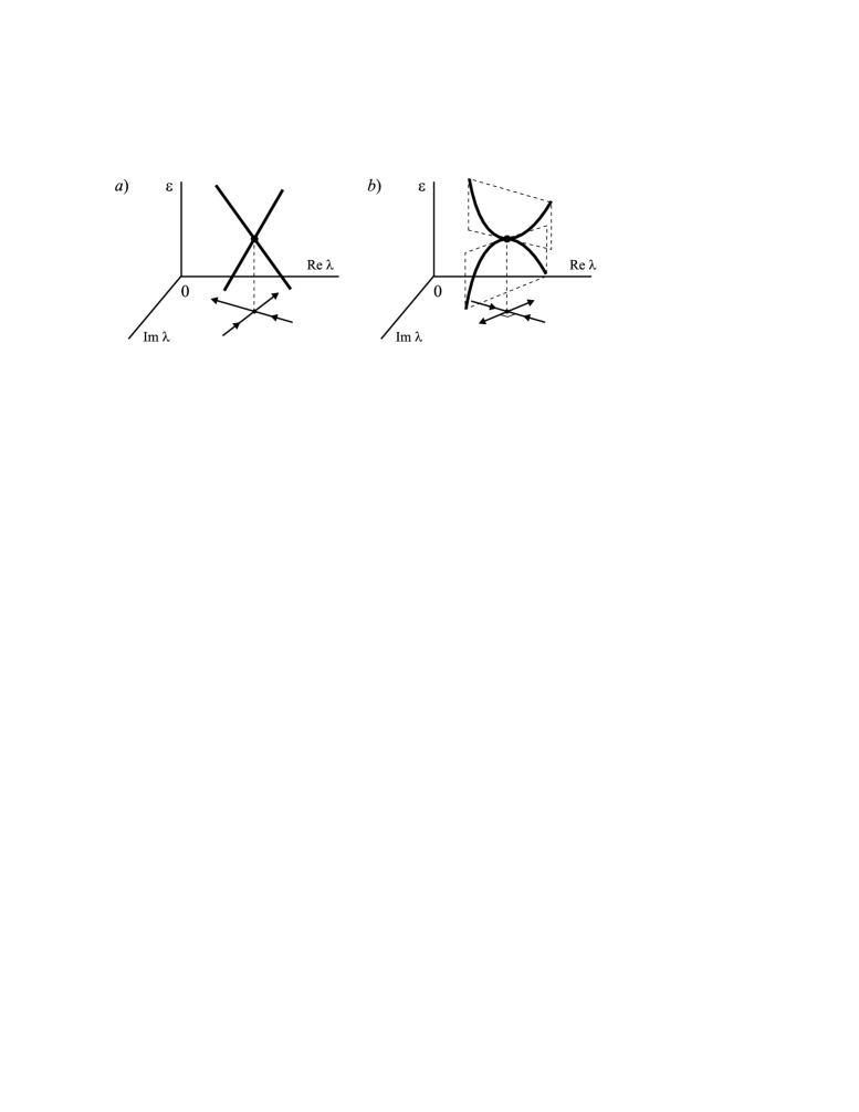
Figure 1: Eigenvalue coupling: (a) weak, (b) strong.

2.2 Strong coupling of eigenvalues

Let us consider coupling of eigenvalues at $\mathbf{p}_{0}$ with a double eigenvalue $\lambda_{0}$ possessing a single eigenvector $\mathbf{u}_{0}$. This case corresponds to the exceptional point. The second vector of the invariant subspace corresponding to $\lambda_{0}$ is called an associated vector $\mathbf{u}_{1}$ (also called a generalized eigenvector [Lancaster (1969)]); it is determined by the equation

$$\mathbf{A}_{0}\mathbf{u}_{1}=\lambda_{0}\mathbf{u}_{1}+\mathbf{u}_{0}.$$ (8)

An eigenvector $\mathbf{v}_{0}$ and an associated vector $\mathbf{v}_{1}$ of the matrix $\mathbf{A}^{*}$ are determined by

$$\mathbf{A}_{0}^{*}\mathbf{v}_{0}=\overline{\lambda}_{0}\mathbf{v}_{0},\quad\mathbf{A}_{0}^{*}\mathbf{v}_{1}=\overline{\lambda}_{0}\mathbf{v}_{1}+\mathbf{v}_{0},\quad(\mathbf{u}_{1},\mathbf{v}_{0})=1,\quad(\mathbf{u}_{1},\mathbf{v}_{1})=0,$$ (9)

where the last two equations are the normalization conditions determining $\mathbf{v}_{0}$ and $\mathbf{v}_{1}$ uniquely for a given $\mathbf{u}_{1}$.

Bifurcation of $\lambda_{0}$ into two eigenvalues $\lambda_{\pm}$ and the corresponding eigenvectors $\mathbf{u}_{\pm}$ are described by (see e.g. [Seyranian and Mailybaev (2003)])

$$\begin{array}[]{rcl}\lambda_{\pm}&=&\lambda_{0}\pm\sqrt{\mu_{1}\varepsilon}+\mu_{2}\varepsilon+o(\varepsilon),\\[5.0pt] \mathbf{u}_{\pm}&=&\mathbf{u}_{0}\pm\mathbf{u}_{1}\sqrt{\mu_{1}\varepsilon}+(\mu_{1}\mathbf{u}_{0}+\mu_{2}\mathbf{u}_{1}-\mathbf{G}^{-1}\mathbf{A}_{1}\mathbf{u}_{0})\varepsilon+o(\varepsilon),\end{array}$$ (10)

where $\mathbf{G}=\mathbf{A}_{0}-\lambda_{0}\mathbf{I}+\mathbf{u}_{1}\mathbf{v}_{1}^{*}$. The coefficients $\mu_{1}$ and $\mu_{2}$ are

$$\mu_{1}=(\mathbf{A}_{1}\mathbf{u}_{0},\mathbf{v}_{0}),\quad\mu_{2}=\big{(}(\mathbf{A}_{1}\mathbf{u}_{0},\mathbf{v}_{1})+(\mathbf{A}_{1}\mathbf{u}_{1},\mathbf{v}_{0})\big{)}/2.$$ (11)

With a change of $\varepsilon$ from negative to positive values, the two eigenvalues $\lambda_{\pm}$ approach, collide with infinite speed (derivative with respect to $\varepsilon$ tends to infinity) at $\lambda_{0}$, and diverge in the perpendicular direction, see Figure 1b. The eigenvectors interact too. At $\varepsilon=0$, they merge to $\mathbf{u}_{0}$ up to a scalar complex factor. At nonzero $\varepsilon$, the eigenvectors $\mathbf{u}_{\pm}$ differ from $\mathbf{u}_{0}$ by the leading term $\pm\mathbf{u}_{1}\sqrt{\mu_{1}\varepsilon}$. This term takes the purely imaginary factor $i$ as $\varepsilon$ changes the sign, for example altering from negative to positive values.

We call such a coupling of eigenvalues as strong. An exciting feature of the strong coupling is that the two eigenvalues cannot be distinguished after the interaction. Indeed, there is no natural rule telling how the eigenvalues before coupling correspond to those after the coupling.

3 Crossing of eigenvalue surfaces

3.1 Double eigenvalue with single eigenvector

Let, at the point ${\bf p}_{0}$, the spectrum of the complex matrix family ${\bf A}({\bf p})$ contain a double complex eigenvalue $\lambda_{0}$ with an eigenvector ${\bf u}_{0}$ and an associated vector ${\bf u}_{1}$. The splitting of the double eigenvalue with a change of the parameters is governed by equations (10) and (11). Introducing the real $n$-dimensional vectors $\bf f$, $\bf g$, $\bf h$, $\bf r$ with the components

$${f}_{s}={\rm Re}\left(\frac{\partial\bf A}{\partial p_{s}}{\bf u}_{0},{\bf v}_{0}\right),~{}~{}{g}_{s}={\rm Im}\left(\frac{\partial\bf A}{\partial p_{s}}{\bf u}_{0},{\bf v}_{0}\right),$$ (12)

$${h}_{s}={\rm Re}\left(\left(\frac{\partial\bf A}{\partial p_{s}}{\bf u}_{0},{\bf v}_{1}\right)+\left(\frac{\partial\bf A}{\partial p_{s}}{\bf u}_{1},{\bf v}_{0}\right)\right),~{}~{}{r}_{s}={\rm Im}\left(\left(\frac{\partial\bf A}{\partial p_{s}}{\bf u}_{0},{\bf v}_{1}\right)+\left(\frac{\partial\bf A}{\partial p_{s}}{\bf u}_{1},{\bf v}_{0}\right)\right),$$ (13)

$$s=1,\ldots,n.$$

and neglecting higher order terms, we obtain from (10) an asymptotic formula

$${\rm Re}\Delta\lambda+i{\rm Im}\Delta\lambda=\pm\sqrt{\langle{\bf f},\Delta{\bf p}\rangle+i\langle{\bf g},\Delta{\bf p}\rangle}+\frac{1}{2}(\langle{\bf h},\Delta{\bf p}\rangle+i\langle{\bf r},\Delta{\bf p}\rangle),$$ (14)

where $\Delta\lambda=\lambda_{\pm}-\lambda_{0}$, $\Delta{\bf p}={\bf p}-{\bf p}_{0}$, and angular brackets denote inner product of real vectors: $\langle{\bf a},{\bf b}\rangle=\sum_{s=1}^{n}a_{s}b_{s}$. From equation (14) it is clear that the eigenvalue remains double in the first approximation if the two following equations are satisfied

$$\langle{\bf f},\Delta{\bf p}\rangle=0,~{}~{}\langle{\bf g},\Delta{\bf p}\rangle=0.$$ (15)

This means that the double complex eigenvalue with the Jordan chain of length 2 has codimension 2. Thus, double complex eigenvalues occur at isolated points of the plane of two parameters, and in the three-parameter space the double eigenvalues form a curve [Arnold (1983)]. Equations (15) define a tangent line to this curve at the point ${\bf p}_{0}$.

Taking square of (14), where the terms linear with respect to the increment of parameters are neglected, and separating real and imaginary parts, we derive the equations

$$({\rm Re}\Delta\lambda)^{2}-({\rm Im}\Delta\lambda)^{2}=\langle{\bf f},\Delta{\bf p}\rangle,~{}~{}2{\rm Re}\Delta\lambda\,{\rm Im}\Delta\lambda=\langle{\bf g},\Delta{\bf p}\rangle.$$ (16)

Let us assume that $f_{1}^{2}+g_{1}^{2}\neq 0$, which is the nondegeneracy condition for the complex eigenvalue $\lambda_{0}$. Isolating the increment $\Delta p_{1}$ in one of the equations (16) and substituting it into the other one we get

$$g_{1}({\rm Re}\Delta\lambda)^{2}-2f_{1}{\rm Re}\Delta\lambda\,{\rm Im}\Delta\lambda-g_{1}({\rm Im}\Delta\lambda)^{2}=\gamma,$$ (17)

where $\gamma$ is a small real constant

$$\gamma=\sum_{s=2}^{n}(f_{s}g_{1}-f_{1}g_{s})\Delta p_{s}.$$ (18)

Equation (17) describes hyperbolic trajectories of the eigenvalues $\lambda_{\pm}$ in the complex plane when only $\Delta p_{1}$ is changed and the increments $\Delta p_{2}$, $\ldots$, $\Delta p_{n}$ are fixed. Of course, any component of the vector $\Delta{\bf p}$ can be chosen instead of $\Delta p_{1}$.

Let us study movement of eigenvalues in the complex plane in more detail. If $\Delta p_{j}=0$, $j=2,\ldots,n$, or if they are nonzero but satisfy the equality $\gamma=0$, then equation (17) yields two perpendicular lines which for $g_{1}\neq 0$ are described by the expression

$$g_{1}{\rm Re}(\lambda-\lambda_{0})-\left(f_{1}\pm\sqrt{f_{1}^{2}+g_{1}^{2}}\right){\rm Im}(\lambda-\lambda_{0})=0.$$ (19)

These lines intersect at the point $\lambda_{0}$ of the complex plane. Due to variation of the parameter $p_{1}$ two eigenvalues $\lambda_{\pm}$ approach along one of the lines (19), merge to $\lambda_{0}$ at $\Delta p_{1}=0$, and then diverge along the other line (19), perpendicular to the line of approach; see Figure 2b, where the arrows show motion of eigenvalues with a monotonous change of $p_{1}$. Recall that the eigenvalues that born after the coupling cannot be identified with the eigenvalues before the coupling.

If $\gamma\neq 0$, then equation (17) defines a hyperbola in the complex plane. Indeed, for $g_{1}\neq 0$ it is transformed to the equation of hyperbola

$$(g_{1}{\rm Re}(\lambda-\lambda_{0})-f_{1}{\rm Im}(\lambda-\lambda_{0}))^{2}-({\rm Im}(\lambda-\lambda_{0}))^{2}(f_{1}^{2}+g_{1}^{2})=\gamma g_{1}$$ (20)

with the asymptotes described by equation (19). As $\Delta p_{1}$ changes monotonously, two eigenvalues $\lambda_{+}$ and $\lambda_{-}$ moving each along its own branch of hyperbola come closer, turn and diverge; see Figure 2a,c. Note that for a small $\gamma$ the eigenvalues $\lambda_{\pm}$ come arbitrarily close to each other without coupling that means avoided crossing. When $\gamma$ changes the sign, the quadrants containing hyperbola branches are changed to the adjacent.

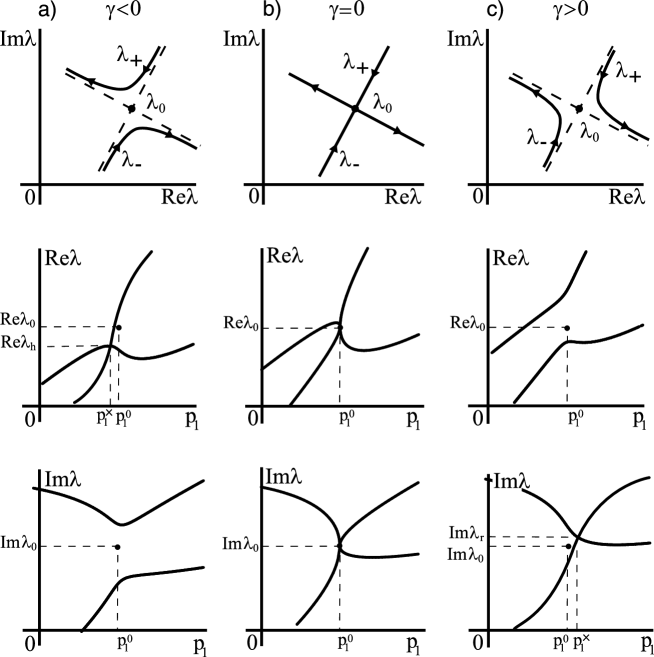
Figure 2: Crossing and avoided crossing of eigenvalues.

Expressing ${\rm Im}\Delta\lambda$ from the second of equations (16), substituting it into the first equation and then isolating ${\rm Re}\Delta\lambda$, we find

$${\rm Re}\lambda_{\pm}=\lambda_{0}+\frac{1}{2}\langle{\bf h},\Delta{\bf p}\rangle\pm\sqrt{\frac{1}{2}\left(\langle{\bf f},\Delta{\bf p}\rangle+\sqrt{\langle{\bf f},\Delta{\bf p}\rangle^{2}+\langle{\bf g},\Delta{\bf p}\rangle^{2}}\right)}.$$ (21)

Similar transformation yields

$${\rm Im}\lambda_{\pm}=\lambda_{0}+\frac{1}{2}\langle{\bf r},\Delta{\bf p}\rangle\pm\sqrt{\frac{1}{2}\left(-\langle{\bf f},\Delta{\bf p}\rangle+\sqrt{\langle{\bf f},\Delta{\bf p}\rangle^{2}+\langle{\bf g},\Delta{\bf p}\rangle^{2}}\right)}.$$ (22)

Equations (21) and (22) describe behavior of real and imaginary parts of eigenvalues $\lambda_{\pm}$ with a change of the parameters. On the other hand they define hypersurfaces in the spaces $(p_{1},p_{2},\ldots,p_{n},{\rm Re}\lambda)$ and $(p_{1},p_{2},\ldots,p_{n},{\rm Im}\lambda)$. The sheets ${\rm Re}\lambda_{+}(\bf p)$ and ${\rm Re}\lambda_{-}(\bf p)$ of the eigenvalue hypersurface (21) are connected at the points of the set

$${\rm Re}\Delta\lambda=\frac{1}{2}\langle{\bf h},\Delta{\bf p}\rangle,~{}~{}\langle{\bf g},\Delta{\bf p}\rangle=0,~{}~{}\langle{\bf f},\Delta{\bf p}\rangle\leq 0,$$ (23)

where the real parts of the eigenvalues $\lambda_{\pm}$ coincide: ${\rm Re}\lambda_{-}={\rm Re}\lambda_{+}$. Similarly, the set

$${\rm Im}\Delta\lambda=\frac{1}{2}\langle{\bf r},\Delta{\bf p}\rangle,~{}~{}\langle{\bf g},\Delta{\bf p}\rangle=0,~{}~{}\langle{\bf f},\Delta{\bf p}\rangle\geq 0,$$ (24)

glues the sheets ${\rm Im}\lambda_{+}(\bf p)$ and ${\rm Im}\lambda_{-}(\bf p)$ of the eigenvalue hypersurface (22).

To study the geometry of the eigenvalue hypersurfaces we look at their two-dimensional cross-sections. Consider for example the functions ${\rm Re}\lambda(p_{1})$ and ${\rm Im}\lambda(p_{1})$ at fixed values of the other parameters $p_{2},p_{3},\ldots,p_{n}$. When the increments $\Delta p_{s}=0$, $s=2,3,\ldots,n$, both the real and imaginary parts of the eigenvalues $\lambda_{\pm}$ cross at $p_{1}=p_{1}^{0}$, see Figure 2b. The crossings are described by the double cusps defined by the equations following from (21) and (22) as

$${\rm Re}\Delta\lambda=\pm\sqrt{\frac{f_{1}\pm\sqrt{f_{1}^{2}+g_{1}^{2}}}{2}\Delta p_{1}}+\frac{h_{1}}{2}\Delta p_{1},~{}~{}{\rm Im}\Delta\lambda=\pm\sqrt{\frac{-f_{1}\pm\sqrt{f_{1}^{2}+g_{1}^{2}}}{2}\Delta p_{1}}+\frac{r_{1}}{2}\Delta p_{1}.$$ (25)

For the fixed $\Delta p_{s}\neq 0$, $s=2,3,\ldots,n$, either real parts of the eigenvalues $\lambda_{\pm}$ cross due to variation of $p_{1}$ while the imaginary parts avoid crossing or vice-versa, as shown in Figure 2a,c. Note that these two cases correspond to level crossing and width repulsion or vice-versa studied in [Heiss (2000)]. The crossings, which occur at $p_{1}^{\times}=p_{1}^{0}-\sum_{s=2}^{n}(g_{s}/g_{1})\Delta p_{s}$ and

$${\rm Re}\lambda_{h}={\rm Re}\lambda_{0}-\frac{1}{2g_{1}}\sum_{s=2}^{n}(h_{1}g_{s}-g_{1}h_{s})\Delta p_{s},~{}~{}{\rm Im}\lambda_{r}={\rm Im}\lambda_{0}-\frac{1}{2g_{1}}\sum_{s=2}^{n}(r_{1}g_{s}-g_{1}r_{s})\Delta p_{s},$$ (26)

are described by the equations (21) and (22). In the vicinity of the crossing points the tangents of two intersecting curves are

$${\rm Re}\lambda={\rm Re}\lambda_{h}+\left(\frac{h_{1}}{2}\pm\frac{g_{1}}{2}\sqrt{\frac{g_{1}}{\gamma}}\right)(p_{1}-p_{1}^{\times}),$$ (27)

$${\rm Im}\lambda={\rm Im}\lambda_{r}+\left(\frac{r_{1}}{2}\pm\frac{g_{1}}{2}\sqrt{-\frac{g_{1}}{\gamma}}\right)(p_{1}-p_{1}^{\times}),$$ (28)

where the coefficient $\gamma$ is defined by equation (18). Lines (27) and (28) tend to the vertical position as $\gamma\rightarrow 0$ and coincide at $\gamma=0$. The avoided crossings are governed by the equations (21) and (22).

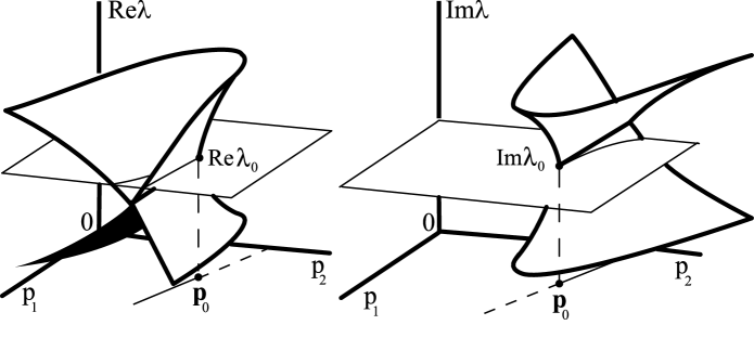
Figure 3: Crossing of eigenvalue surfaces near the double eigenvalue with single eigenvector.

If the vector of parameters consists of only two components ${\bf p}=(p_{1},p_{2})$, then in the vicinity of the point ${\bf p}_{0}$, corresponding to the double eigenvalue $\lambda_{0}$, the eigenvalue surfaces (21) and (22) have the form of the well-known Whitney umbrella; see Figure 3. The sheets of the eigensurfaces are connected along the rays (23) and (24). We emphasize that these rays are inclined with respect to the plane of the parameters $p_{1}$, $p_{2}$. The cross-sections of the eigensurfaces by the planes orthogonal to the axis $p_{2}$, described by the equations (25)–(28), are shown in Figure 2.

Note that the rays (23), (24) and the point ${\bf p}_{0}$ are well-known in crystal optics as the branch cuts and the singular axis, respectively [Berry and Dennis (2003)]. We emphasize that the branch cut is a general phenomenon: it always appears near the EP degeneracy. In general, branch cuts may be infinite or end up at another EP. The second scenario is always the case when the complex matrix $\mathbf{A}(\mathbf{p})$ is a small perturbation of a family of real symmetric matrices [Kirillov et al. (2004)].

Consider the movement of the eigenvalues in the complex plane near the point ${\bf p}_{0}$ due to cyclic variation of the parameters $p_{1}$ and $p_{2}$ of the form $\Delta p_{1}=a+r\cos{\varphi}$ and $\Delta p_{2}=b+r\sin{\varphi}$, where $a$, $b$, and $r$ are small parameters of the same order. From equations (16) we derive

$$(g_{1}{\rm Re}\Delta\lambda^{2}-2f_{1}{\rm Re}\Delta\lambda{\rm Im}\Delta\lambda-g_{1}{\rm Im}\Delta\lambda^{2}-b(f_{2}g_{1}-f_{1}g_{2}))^{2}+$$

$$+(g_{2}{\rm Re}\Delta\lambda^{2}-2f_{2}{\rm Re}\Delta\lambda{\rm Im}\Delta\lambda-g_{2}{\rm Im}\Delta\lambda^{2}-a(f_{1}g_{2}-g_{1}f_{2}))^{2}=(f_{2}g_{1}-f_{1}g_{2})^{2}r^{2}.$$ (29)

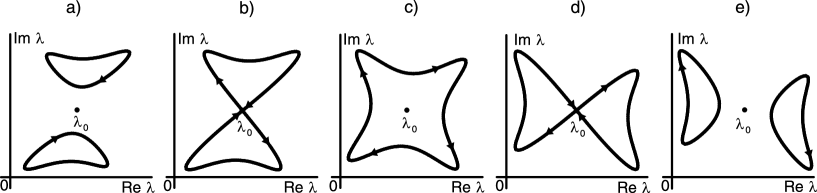
Figure 4: Movement of eigenvalues due to cyclic evolution of the parameters.

Movement of eigenvalues on the complex plane governed by equation (29) is shown in Figure 4. If the contour encircles the point ${\bf p}_{0}$, then the eigenvalues move along the curve (29) around the double eigenvalue $\lambda_{0}$ in the complex plane, see Figure 4c. Indeed, in this case $a^{2}+b^{2}<r^{2}$ and the loop (29) crosses the lines ${\rm Re}\lambda={\rm Re}\lambda_{0}$ and ${\rm Im}\lambda={\rm Im}\lambda_{0}$ at the four points given by the equations

$$({\rm Im}\Delta\lambda)^{2}=\frac{(f_{2}g_{1}-f_{1}g_{2})\left(g_{2}a-g_{1}b\pm\sqrt{(g_{2}a-g_{1}b)^{2}+(r^{2}-a^{2}-b^{2})(g_{1}^{2}+g_{2}^{2})}\right)}{g_{1}^{2}+g_{2}^{2}}$$ (30)

and

$$({\rm Re}\Delta\lambda)^{2}=\frac{(f_{2}g_{1}-f_{1}g_{2})\left(g_{1}b-g_{2}a\pm\sqrt{(g_{1}b-g_{2}a)^{2}+(r^{2}-a^{2}-b^{2})(g_{1}^{2}+g_{2}^{2})}\right)}{g_{1}^{2}+g_{2}^{2}},$$ (31)

respectively. When $a^{2}+b^{2}=r^{2}$ the loop overlaps at the double eigenvalue and its form depends on the sign of the quantity $\sigma=(f_{2}g_{1}-f_{1}g_{2})(g_{1}b-g_{2}a)$. If $\sigma<0$ the eigenvalues cross the line ${\rm Re}\lambda={\rm Re}\lambda_{0}$ (Figure 4b), otherwise they cross the line ${\rm Im}\lambda={\rm Im}\lambda_{0}$ (Figure 4d). Eigenvalues strongly couple at the point $\lambda_{0}$ in the complex plane. For $a^{2}+b^{2}>r^{2}$ the circuit in the parameter plane does not contain the point ${\bf p}_{0}$ and the eigenvalues move along the two different closed paths (”kidneys”, [Arnold (1989)]) in the complex plane, see Figure 4a,e. Each eigenvalue crosses the line ${\rm Re}\lambda={\rm Re}\lambda_{0}$ twice for $\sigma<0$ (Figure 4a), and for $\sigma>0$ they cross the line ${\rm Im}\lambda={\rm Im}\lambda_{0}$ (Figure 4d). Note that the ”kidneys” in the complex plane were observed in [Korsch and Mossman (2003)] for the specific problem of Stark resonances for a double $\delta$ quantum well.

3.2 Double eigenvalue with two eigenvectors

Let $\lambda_{0}$ be a double eigenvalue of the matrix $\mathbf{A}_{0}=\mathbf{A}(\mathbf{p}_{0})$ with two eigenvectors $\mathbf{u}_{1}$ and $\mathbf{u}_{2}$. Under perturbation of parameters $\mathbf{p}=\mathbf{p}_{0}+\Delta\mathbf{p}$, the bifurcation of $\lambda_{0}$ into two simple eigenvalues $\lambda_{+}$ and $\lambda_{-}$ occurs. Using (5) and (7), we obtain the asymptotic formula for $\lambda_{\pm}$ under multiparameter perturbation as

$$\lambda_{\pm}=\lambda_{0}+\frac{\langle\mathbf{d}_{11}+\mathbf{d}_{22},\Delta\mathbf{p}\rangle}{2}\pm\sqrt{\frac{\langle\mathbf{d}_{11}-\mathbf{d}_{22},\Delta\mathbf{p}\rangle^{2}}{4}+\langle\mathbf{d}_{12},\Delta\mathbf{p}\rangle\langle\mathbf{d}_{21},\Delta\mathbf{p}\rangle},$$ (32)

where $\mathbf{d}_{ij}=(d_{ij}^{1},\ldots,d_{ij}^{n})$ is a complex vector with the components

$$d_{ij}^{k}=\left(\frac{\partial\mathbf{A}}{\partial p_{k}}\mathbf{u}_{i},\mathbf{v}_{j}\right),$$ (33)

and $\langle\mathbf{d}_{ij},\Delta\mathbf{p}\rangle=\langle\mathrm{Re}\,\mathbf{d}_{ij},\Delta\mathbf{p}\rangle+i\langle\mathrm{Im}\,\mathbf{d}_{ij},\Delta\mathbf{p}\rangle$. In the same way as we derived formulae (21) and (22), we obtain from (32) the expressions for real and imaginary parts of $\lambda_{\pm}$ in the form

$$\mathrm{Re}\,\lambda_{\pm}=\mathrm{Re}\,\lambda_{0}+\mathrm{Re}\,\langle\mathbf{d}_{11}+\mathbf{d}_{22},\Delta\mathbf{p}\rangle/2\pm\sqrt{(|c|+\mathrm{Re}\,c)/2},$$ (34)

$$\mathrm{Im}\,\lambda_{\pm}=\mathrm{Im}\,\lambda_{0}+\mathrm{Im}\,\langle\mathbf{d}_{11}+\mathbf{d}_{22},\Delta\mathbf{p}\rangle/2\pm\sqrt{(|c|-\mathrm{Re}\,c)/2},$$ (35)

where

$$c=\langle\mathbf{d}_{11}-\mathbf{d}_{22},\Delta\mathbf{p}\rangle^{2}/4+\langle\mathbf{d}_{12},\Delta\mathbf{p}\rangle\langle\mathbf{d}_{21},\Delta\mathbf{p}\rangle.$$ (36)

Considering the situation when $\lambda_{0}$ remains double under perturbation of parameters, i.e. $\lambda_{+}=\lambda_{-}$, we obtain the two independent equations

$$\mathrm{Re}\,c=0,\quad\mathrm{Im}\,c=0.$$ (37)

By using (5)–(7), one can show that the perturbed double eigenvalue $\lambda_{+}=\lambda_{-}$ possesses a single eigenvector $\mathbf{u}_{+}=\mathbf{u}_{-}$, i.e., the weak coupling becomes strong due to perturbation, see [Seyranian and Mailybaev (2003)].

The perturbed double eigenvalue has two eigenvectors only when the matrix in the left-hand side of (6) is proportional to the identity matrix. This yields the equations

$$\langle\mathbf{d}_{11},\Delta\mathbf{p}\rangle=\langle\mathbf{d}_{22},\Delta\mathbf{p}\rangle,\quad\langle\mathbf{d}_{12},\Delta\mathbf{p}\rangle=\langle\mathbf{d}_{21},\Delta\mathbf{p}\rangle=0,$$ (38)

Conditions (38) imply (37) and represent six independent equations taken for real and imaginary parts. Thus, weak coupling of eigenvalues is a phenomenon of codimension 6, which generically occurs at isolated points in 6-parameter space, see [Arnold (1983), Mondragon and Hernandez (1993)].

First, let us study behavior of the eigenvalues $\lambda_{+}$ and $\lambda_{-}$ depending on one parameter, say $p_{1}$, when the other parameters $p_{2},\ldots,p_{n}$ are fixed in the neighborhood of the coupling point $\lambda_{+}(\mathbf{p}_{0})=\lambda_{-}(\mathbf{p}_{0})=\lambda_{0}$. In case $\Delta p_{2}=\cdots=\Delta p_{n}=0$, expression (32) yields

$$\lambda_{\pm}=\lambda_{0}+\left(\frac{d_{11}^{1}+d_{22}^{1}}{2}\pm\sqrt{\frac{(d_{11}^{1}-d_{22}^{1})^{2}}{4}+d_{12}^{1}d_{21}^{1}}\right)\Delta p_{1}.$$ (39)

The two eigenvalues couple when $\Delta p_{1}=0$ with the double eigenvalue $\lambda_{0}$, see Figure 5a. As we showed in Section 2, the eigenvalues $\lambda_{+}$ and $\lambda_{-}$ behave as smooth functions at the coupling point; they possess different eigenvectors, which are smooth functions of $\Delta p_{1}$ too.

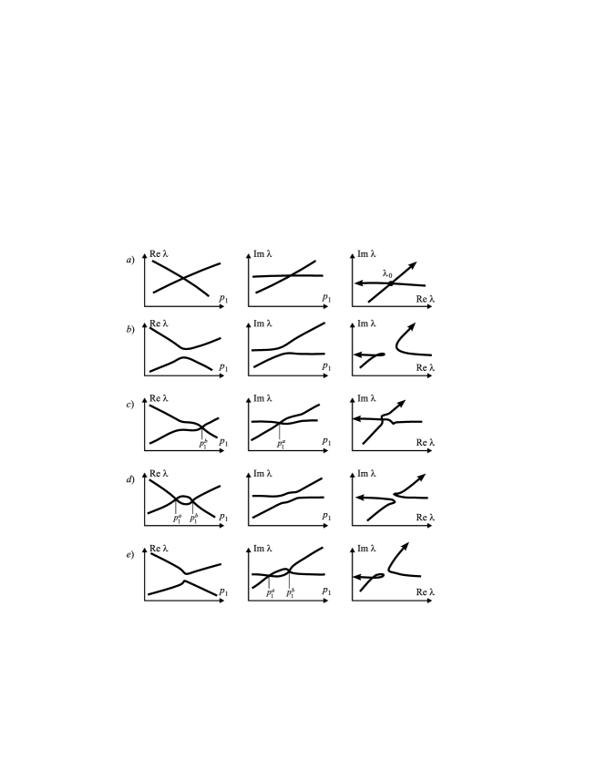
Figure 5: Weak coupling of eigenvalues and avoided crossing.

If the perturbations $\Delta p_{2},\ldots,\Delta p_{n}$ are nonzero, the avoided crossing of the eigenvalues $\lambda_{\pm}$ with a change of $p_{1}$ is a typical scenario. We can distinguish different cases by checking intersections of real and imaginary parts of $\lambda_{+}$ and $\lambda_{-}$. By using (34), we find that $\mathrm{Re}\,\lambda_{+}=\mathrm{Re}\,\lambda_{-}$ if

$$\mathrm{Im}\,c=0,\quad\mathrm{Re}\,c<0.$$ (40)

Analogously, from (35) it follows that $\mathrm{Im}\,\lambda_{+}=\mathrm{Im}\,\lambda_{-}$ if

$$\mathrm{Im}\,c=0,\quad\mathrm{Re}\,c>0.$$ (41)

Let us write expression (36) in the form

$$c=c_{0}+c_{1}\Delta p_{1}+c_{2}(\Delta p_{1})^{2},$$ (42)

where

$$\begin{array}[]{c}c_{0}=\displaystyle\sum_{k,l=2}^{n}\left[(d_{11}^{k}-d_{22}^{k})(d_{11}^{l}-d_{22}^{l})/4+d_{12}^{k}d_{21}^{l}\right]\Delta p_{k}\Delta p_{l},\\[15.0pt] c_{1}=\displaystyle\sum_{k=2}^{n}\left[(d_{11}^{1}-d_{22}^{1})(d_{11}^{k}-d_{22}^{k})/2+(d_{12}^{1}d_{21}^{k}+d_{12}^{k}d_{21}^{1})\right]\Delta p_{k},\\[12.0pt] c_{2}=(d_{11}^{1}-d_{22}^{1})^{2}/4+d_{12}^{1}d_{21}^{1}.\end{array}$$ (43)

If the discriminant $D=(\mathrm{Im}\,c_{1})^{2}-4\mathrm{Im}\,c_{0}\mathrm{Im}\,c_{2}>0$, the equation $\mathrm{Im}\,c=0$ yields two solutions

$$\Delta p_{1}^{a}=\frac{-\mathrm{Im}\,c_{1}-\sqrt{D}}{2\mathrm{Im}\,c_{2}},\quad\Delta p_{1}^{b}=\frac{-\mathrm{Im}\,c_{1}+\sqrt{D}}{2\mathrm{Im}\,c_{2}}.$$ (44)

There are no real solutions if $D<0$, and the single solution corresponds to the degenerate case $D=0$. At the points $p_{1}^{a}=p_{1}^{0}+\Delta p_{1}^{a}$ and $p_{1}^{b}=p_{1}^{0}+\Delta p_{1}^{b}$ the values of $c$ are real, and we denote them by $c_{a}$ and $c_{b}$, respectively. According to (40) and (41), the sign of $c_{a,b}$ determines whether the real or imaginary parts of $\lambda_{\pm}$ coincide at $p_{1}^{a,b}$.

In the nondegenerate case $D\neq 0$, there are four types of avoided crossing shown in Figure 5b–e. The first case corresponds to $D<0$ when both real and imaginary parts of the eigenvalues $\lambda_{\pm}$ are separate at all $p_{1}$, see Figure 5b. In other cases $D>0$, so that there are two separate points $p_{1}^{a}$ and $p_{1}^{b}$. For the second type we have $c_{a}>0$ and $c_{b}<0$, when both real and imaginary parts of $\lambda_{\pm}$ have a single intersection, see Figure 5c. The equivalent situation when $c_{a}<0$ and $c_{b}>0$ is obtained by interchanging the points $p_{1}^{a}$ and $p_{1}^{b}$ in Figure 5c. The third type is represented by $c_{a,b}<0$, when the real parts of $\lambda_{\pm}$ have two intersections and $\mathrm{Im}\,\lambda_{\pm}$ do not intersect, see Figure 5d. Finally, if $c_{a,b}>0$, when the real parts of $\lambda_{\pm}$ do not intersect and $\mathrm{Im}\,\lambda_{\pm}$ intersect at both $p_{1}^{a}$ and $p_{1}^{b}$, see Figure 5e. The last column in Figure 5 shows behavior of the eigenvalues $\lambda_{\pm}$ on the complex plane. In each of the cases b–e, the trajectories of eigenvalues on the complex plane may intersect and/or self-intersect, which can be studied by using expression (32). Note that intersections of the eigenvalue trajectories on the complex plane do not imply eigenvalue coupling since the eigenvalues $\lambda_{+}$ and $\lambda_{-}$ pass the intersection point at different values of $p_{1}$. The small loops of the eigenvalue trajectories on the complex plane, shown in Figure 5b,e, shrink as the perturbations of the parameters $\Delta p_{2},\Delta p_{3},\ldots,\Delta p_{n}$ tend to zero. Finally, we mention that the case of Figure 5c is the only avoided crossing scenario when the eigenvalues follow the initial directions on the complex plane after interaction. In the other three cases (b,d, and e) the eigenvalues interchange their directions due the interaction.

Let us consider a system depending on two parameters $p_{1}$ and $p_{2}$ with the weak coupling of eigenvalues at $p_{1}=p_{1}^{0}$ and $p_{2}=p_{2}^{0}$. The double eigenvalue $\lambda_{0}$ bifurcates into a pair $\lambda_{\pm}$ under perturbation of the parameters $\Delta p_{1}$ and $\Delta p_{2}$. Conditions (40) and (41) determine the values of parameters, at which the real and imaginary parts of $\lambda_{\pm}$ coincide.

Let us write expression (36) in the form

$$c=c_{11}(\Delta p_{1})^{2}+c_{12}\Delta p_{1}\Delta p_{2}+c_{22}(\Delta p_{2})^{2},$$ (45)

where

$$\begin{array}[]{c}c_{11}=(d_{11}^{1}-d_{22}^{1})^{2}/4+d_{12}^{1}d_{21}^{1},\quad c_{22}=(d_{11}^{2}-d_{22}^{2})^{2}/4+d_{12}^{2}d_{21}^{2},\\[5.0pt] c_{12}=(d_{11}^{1}-d_{22}^{1})(d_{11}^{2}-d_{22}^{2})/2+d_{12}^{1}d_{21}^{2}+d_{12}^{2}d_{21}^{1}.\end{array}$$ (46)

If the discriminant $D^{\prime}=(\mathrm{Im}\,c_{12})^{2}-4\mathrm{Im}\,c_{11}\mathrm{Im}\,c_{22}>0$, the equation $\mathrm{Im}\,c=0$ yields the two crossing lines

$$\begin{array}[]{l}l_{a}:\ \ 2\mathrm{Im}\,c_{11}\Delta p_{1}+(\mathrm{Im}\,c_{12}+\sqrt{D^{\prime}})\Delta p_{2}=0,\\[5.0pt] l_{b}:\ \ 2\mathrm{Im}\,c_{11}\Delta p_{1}+(\mathrm{Im}\,c_{12}-\sqrt{D^{\prime}})\Delta p_{2}=0.\end{array}$$ (47)

There are no real solutions if $D^{\prime}<0$, and the lines $l_{a}$ and $l_{b}$ coincide in the degenerate case $D^{\prime}=0$. On the lines $l_{a,b}$ the values of $c$ are real numbers of the same sign; we denote $\gamma_{a}=\mathrm{sign}\,c$ for the line $l_{a}$, and $\gamma_{b}=\mathrm{sign}\,c$ for the line $l_{b}$. According to (40) and (41), the real or imaginary parts of $\lambda_{\pm}$ coincide at $l_{a,b}$ for negative or positive $\gamma_{a,b}$, respectively.

One can distinguish four types of the graphs for $\mathrm{Re}\,\lambda_{\pm}(p_{1},p_{2})$ and $\mathrm{Im}\,\lambda_{\pm}(p_{1},p_{2})$ shown in Figure 6. In nondegenerate case $D^{\prime}\neq 0$, the eigenvalues $\lambda_{+}$ and $\lambda_{-}$ are different for all parameter values except the initial point $p_{1,2}=p_{1,2}^{0}$. If $D^{\prime}<0$, the eigenvalue surfaces are cones with non-elliptic cross-section, see Figure 6a. Other three types correspond to the case $D^{\prime}>0$. If $\gamma_{a}<0$ and $\gamma_{b}>0$ then there is an intersection of the real parts along the line $l_{a}$ and an intersection of the imaginary parts along the line $l_{b}$ (in case $\gamma_{a}>0$ and $\gamma_{b}<0$ the lines $l_{a}$ and $l_{b}$ are interchanged), see Figure 6b. If $\gamma_{a}<0$ and $\gamma_{b}<0$ then the real parts intersect along the both lines $l_{a}$ and $l_{b}$ forming a ”cluster of shells”, while there is no intersections for the imaginary parts, see Figure 6c. Finally, if $\gamma_{a}>0$ and $\gamma_{b}>0$ then there is no intersections for the real parts, while the imaginary parts intersect along the both lines $l_{a}$ and $l_{b}$, see Figure 6d.

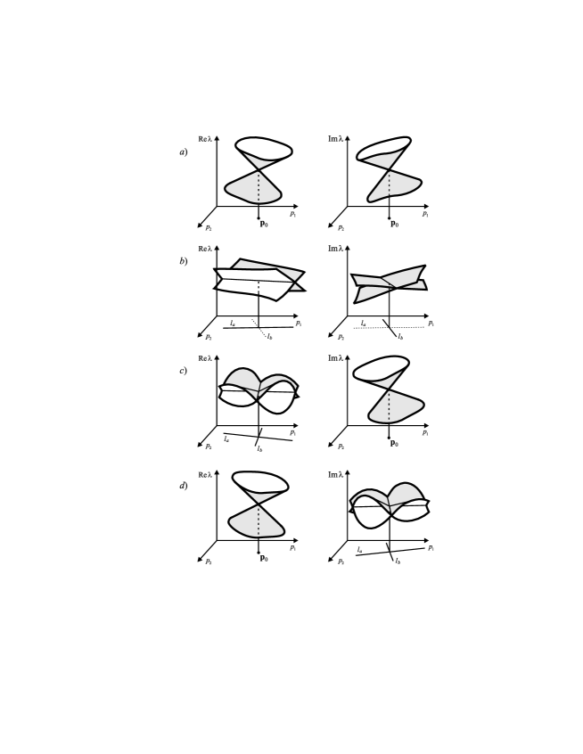
Figure 6: Eigenvalue surfaces near a point of weak coupling.

4 Example

As a physical example, we consider propagation of light in a homogeneous non-magnetic crystal in the general case when the crystal possesses natural optical activity (chirality) and dichroism (absorption) in addition to biaxial birefringence, see [Berry and Dennis (2003)] for the general formulation. The optical properties of the crystal are characterized by the inverse dielectric tensor $\boldsymbol{\eta}$. The vectors of electric field $\bf E$ and displacement $\bf D$ are related as [Landau et al. (1984)]

$${\bf E}={\boldsymbol{\eta}}{\bf D}.$$ (48)

The tensor $\boldsymbol{\eta}$ is described by a non-Hermitian complex matrix. The electric field $\bf E$ and magnetic field $\bf H$ in the crystal are determined by Maxwell’s equations [Landau et al. (1984)]

$${\rm rot}{\bf E}=-\frac{1}{c}\frac{\partial{\bf H}}{\partial t},~{}~{}{\rm rot}{\bf H}=\frac{1}{c}\frac{\partial{\bf D}}{\partial t},$$ (49)

where $t$ is time and $c$ is the speed of light in vacuum.

A monochromatic plane wave of frequency $\omega$ that propagates in a direction specified by a real unit vector ${\bf s}=(s_{1},s_{2},s_{3})$ has the form

$${\bf D}({\bf r},t)={\bf D}({\bf s})\exp i\omega\!\left(\frac{n({\bf s})}{c}{\bf s}^{T}{\bf r}-t\right),\ {\bf H}({\bf r},t)={\bf H}({\bf s})\exp i\omega\!\left(\frac{n({\bf s})}{c}{\bf s}^{T}{\bf r}-t\right),$$ (50)

where $n({\bf s})$ is a refractive index, and ${\bf r}=(x_{1},x_{2},x_{3})$ is the real vector of spatial coordinates. Substituting the wave (50) into Maxwell’s equations (49), we find

$${\bf H}=n[{\bf s},{\boldsymbol{\eta}}{\bf D}],~{}~{}{\bf D}=-n[{\bf s},{\bf H}],$$ (51)

where square brackets indicate cross product of vectors [Landau et al. (1984)]. With the vector $\bf H$ determined by the first equation of (51), the second equation of (51) yields [Berry and Dennis (2003)]

$$-[{\bf s},[{\bf s},{\boldsymbol{\eta}}{\bf D}({\bf s})]]={\boldsymbol{\eta}}{\bf D}({\bf s})-{\bf s}({\bf s}^{T}{\boldsymbol{\eta}}{\bf D}({\bf s}))=\frac{1}{n^{2}({\bf s})}{\bf D}({\bf s}).$$ (52)

Multiplying equation (52) by the vector $\mathbf{s}^{T}$ from the left we find that for plane waves the vector ${\bf D}$ is always orthogonal to the direction $\bf s$, i.e., ${\bf s}^{T}{\bf D}({\bf s})=0$.

Since the quantity ${\bf s}^{T}{\boldsymbol{\eta}}{\bf D}({\bf s})$ is a scalar, we can write (52) in the form of an eigenvalue problem for the complex non-Hermitian matrix $\bf A({\bf s})$ dependent on the vector of parameters ${\bf s}=(s_{1},s_{2},s_{3})$:

$${\bf A}{\bf u}=\lambda{\bf u},~{}~{}{\bf A}({\bf s})=({\bf I}-{\bf s}{\bf s}^{T}){\boldsymbol{\eta}}({\bf s}),$$ (53)

where $\lambda=n^{-2}$, ${\bf u}={\bf D}$, and ${\bf I}$ is the identity matrix. Multiplying the matrix $\bf A$ by the vector $\bf s$ from the left we conclude that ${\bf s}^{T}{\bf A}=0$, i.e., the vector ${\bf s}$ is the left eigenvector with the eigenvalue $\lambda=0$. Zero eigenvalue always exists, because $\det({\bf I}-{\bf s}{\bf s}^{T})\equiv 0$, if $\|{\bf s}\|=1$.

The matrix ${\bf A}({\bf s})$ defined by equation (53) is a product of the matrix ${\bf I}-{\bf s}{\bf s}^{T}$ and the inverse dielectric tensor ${\boldsymbol{\eta}}({\bf s})$. The symmetric part of ${\boldsymbol{\eta}}$ constitutes the anisotropy tensor describing the birefringence of the crystal. It is represented by the complex symmetric matrix $\bf U$, which is independent of the vector of parameters $\bf s$. The antisymmetric part of ${\boldsymbol{\eta}}$ is determined by the optical activity vector ${\bf g}({\bf s})=(g_{1},g_{2},g_{3})$, describing the chirality (optical activity) of the crystal. It is represented by the skew-symmetric matrix

$${\bf G}=i\left(\begin{array}[]{ccc}0&-g_{3}&g_{2}\\ g_{3}&0&-g_{1}\\ -g_{2}&g_{1}&0\\ \end{array}\right).$$ (54)

The vector $\bf g$ is given by the expression ${\bf g}({\bf s})={\boldsymbol{\gamma}}{\bf s}$, where $\boldsymbol{\gamma}$ is the optical activity tensor represented by a symmetric complex matrix. Thus, the matrix $\mathbf{G}(\mathbf{s})$ depends linearly on the parameters $s_{1}$, $s_{2}$, $s_{3}$.

In the present formulation, the problem was studied analytically and numerically in [Berry and Dennis (2003)]. Below we present two specific numerical examples in case of a non-diagonal matrix $\boldsymbol{\gamma}$, for which the structure of singularities was not fully investigated. Unlike [Berry and Dennis (2003)], where the reduction to two dimensions was carried out, we work with the three-dimensional form of problem (53). Our intention here is to give guidelines for using our theory by means of the relatively simple $3\times 3$ matrix family, keeping in mind that the main area of applications would be higher dimensional problems.

As a first example, we choose the inverse dielectric tensor in the form

$${\boldsymbol{\eta}}=\left(\begin{array}[]{ccc}3&0&0\\ 0&1&0\\ 0&0&2\\ \end{array}\right)+i\left(\begin{array}[]{ccc}0&1&2\\ 1&0&0\\ 2&0&0\\ \end{array}\right)+i\left(\begin{array}[]{lll}0&-s_{1}&0\\ s_{1}&0&-s_{3}\\ 0&s_{3}&0\\ \end{array}\right)$$ (55)

where $s_{3}=\sqrt{1-s_{1}^{2}-s_{2}^{2}}$. The crystal defined by (55) is dichroic and optically active with the non-diagonal matrix $\boldsymbol{\gamma}$. When $s_{1}=0$ and $s_{2}=0$ the spectrum of the matrix ${\bf A}$ consists of the double eigenvalue $\lambda_{0}=2$ and the simple zero eigenvalue. The double eigenvalue possesses the eigenvector ${\bf u}_{0}$ and associated vector ${\bf u}_{1}$:

$${\bf u}_{0}=\left(\begin{array}[]{c}i\\ -1\\ 0\\ \end{array}\right),~{}~{}{\bf u}_{1}=\left(\begin{array}[]{c}0\\ 1\\ 0\\ \end{array}\right).$$ (56)

The eigenvector ${\bf v}_{0}$ and associated vector ${\bf v}_{1}$ corresponding to the double eigenvalue $\lambda_{0}=2$ of the adjoint matrix ${\bf A}^{*}$ are

$${\bf v}_{0}=\left(\begin{array}[]{c}i\\ 1\\ 1+i/2\\ \end{array}\right),~{}~{}{\bf v}_{1}=\left(\begin{array}[]{c}i\\ 0\\ 1/2-i/4\\ \end{array}\right).$$ (57)

The vectors ${\bf u}_{0}$, ${\bf u}_{1}$ and ${\bf v}_{0}$, ${\bf v}_{1}$ satisfy the normalization and orthogonality conditions (9). Calculating the derivatives of the matrix ${\bf A}(s_{1},s_{2})$ at the point ${\bf s}_{0}=(0,0,1)$ we obtain

$$\frac{\partial{\bf A}}{\partial s_{1}}=\left(\begin{array}[]{ccc}-2i&-2i&-2\\ i&0&0\\ -3&-i&-2i\\ \end{array}\right),~{}~{}\frac{\partial{\bf A}}{\partial s_{2}}=\left(\begin{array}[]{ccc}0&0&0\\ -2i&-i&-2\\ -i&-1&i\\ \end{array}\right).$$ (58)

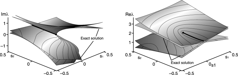
Figure 7: Eigensurfaces of the crystal (55) and their approximations.

Substitution of the derivatives (58) together with the vectors given by equations (56) and (57) into the formulae (12) and (13) yields the vectors ${\bf f}$, ${\bf g}$ and $\bf h$, $\bf r$ as

$${\bf f}=(0,4),~{}~{}{\bf g}=(-4,0),~{}~{}{\bf h}=(0,0),~{}~{}{\bf r}=(-4,0).$$ (59)

With the vectors (59) we find from (21) and (22) the approximations of the eigensurfaces ${\rm Re}\lambda(s_{1},s_{2})$ and ${\rm Im}\lambda(s_{1},s_{2})$ in the vicinity of the point ${\bf s}_{0}=(0,0,1)$:

$${\rm Re}\lambda_{\pm}=2\pm\sqrt{2s_{2}+2\sqrt{s_{1}^{2}+s_{2}^{2}}},~{}~{}{\rm Im}\lambda_{\pm}=-2s_{1}\pm\sqrt{-2s_{2}+2\sqrt{s_{1}^{2}+s_{2}^{2}}}.$$ (60)

Calculation of the exact solution of the characteristic equation for the matrix $\bf A$ with the inverse dielectric tensor $\boldsymbol{\eta}$ defined by equation (55) shows a good agreement of the approximations (60) with the numerical solution, see Figure 7. One can see that the both surfaces of real and imaginary parts have a Whitney umbrella singularity at the coupling point; the surfaces self-intersect along different rays, which together constitute a straight line when projected on parameter plane.

As a second numerical example, let us consider the inverse dielectric tensor as

$${\boldsymbol{\eta}}=\left(\begin{array}[]{ccc}1&0&1\\ 0&1&0\\ 1&0&4\end{array}\right)+i\left(\begin{array}[]{ccc}5&0&4\\ 0&5&2\\ 4&2&0\end{array}\right)+4i\left(\begin{array}[]{ccc}0&-s_{1}-is_{2}&is_{3}\\ s_{1}+is_{2}&0&-s_{3}\\ -is_{3}&s_{3}&0\end{array}\right).$$ (61)

At $\mathbf{s}=(0,0,1)$, the matrix $\mathbf{A}$ has the double eigenvalue $\lambda_{0}=1+5i$ with two eigenvectors and the simple zero eigenvalue. The eigenvectors $\mathbf{u}_{1}$, $\mathbf{u}_{2}$ of $\lambda_{0}$ and the eigenvectors $\mathbf{v}_{1}$, $\mathbf{v}_{2}$ of $\overline{\lambda}_{0}$ for the adjoint matrix $\mathbf{A}^{*}$ are

$$\mathbf{u}_{1}=\left(\begin{array}[]{c}1\\ 0\\ 0\end{array}\right),\quad\mathbf{u}_{2}=\left(\begin{array}[]{c}0\\ 1\\ 0\end{array}\right),\quad\mathbf{v}_{1}=\left(\begin{array}[]{c}1\\ 0\\ \frac{-3-4i}{1-5i}\end{array}\right),\quad\mathbf{v}_{2}=\left(\begin{array}[]{c}0\\ 1\\ \frac{2i}{1-5i}\end{array}\right).$$ (62)

These vectors satisfy normalization conditions (4). Taking derivatives of the matrix $\mathbf{A}$ with respect to parameters $s_{1}$ and $s_{2}$, where $s_{3}=\sqrt{1-s_{1}^{2}-s_{2}^{2}}$, and using formula (33), we obtain

$$\mathbf{d}_{11}=(-2-8i,0),\ \mathbf{d}_{12}=(6i,-9-4i),\ \mathbf{d}_{21}=(-10i,7-4i),\ \mathbf{d}_{22}=(0,-4i).$$ (63)

Using (63) in formulae (34)–(36), we find approximations for real and imaginary parts of two nonzero eigenvalues $\lambda_{\pm}$ near the point $\mathbf{s}=(0,0,1)$ as

$$\mathrm{Re}\,\lambda_{\pm}=1-s_{1}\pm\sqrt{(|c|+\mathrm{Re}\,c)/2},\ \ \mathrm{Im}\,\lambda_{\pm}=5-4s_{1}-2s_{2}\pm\sqrt{(|c|-\mathrm{Re}\,c)/2},$$ (64)

where $c=(45+8i)s_{1}^{2}+128is_{1}s_{2}+(-83+8i)s_{2}^{2}$.

Approximations of eigenvalue surfaces (64) and the exact solutions are presented in Figure 8. The eigenvalue surfaces have intersections both in $(s_{1},s_{2},\mathrm{Re}\,\lambda)$ and $(s_{1},s_{2},\mathrm{Im}\,\lambda)$ spaces. These intersections are represented by two different lines $l_{a}$ and $l_{b}$ in parameter space, see Figure 6b.

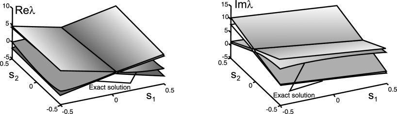
Figure 8: Eigensurfaces of the crystal (61) and their approximations.

5 Conclusion

A general theory of coupling of eigenvalues of complex matrices smoothly depending on multiple real parameters has been presented. Diabolic and exceptional points have been mathematically described and general formulae for coupling of eigenvalues at these points have been derived. This theory gives a clear and complete picture of crossing and avoided crossing of eigenvalues with a change of parameters. It has a very broad field of applications since any physical system contains parameters. It is important that the presented theory of coupling gives not only qualitative, but also quantitative results on eigenvalue surfaces based only on the information at the diabolic and exceptional points. This information includes eigenvalues, eigenvectors and associated vectors with derivatives of the system matrix taken at the singular points. We emphasize that the developed methods provide a firm basis for analysis of spectrum singularities of matrix operators.

6 Acknowledgement

The work is supported by the research grants RFBR-NSFC 02-01-39004, RFBR 03-01-00161, CRDF-BRHE Y1-MP-06-19, and CRDF-BRHE Y1-M-06-03.

References

- [Hamilton (1833)] Hamilton W. R. 1833. On a general Method of expressing the Paths of Light, and of the Planets, by the Coefficients of a Characteristic Function. Dublin University Review and Quarterly Magazine 1, 795–826
- [Berry et al. (1999)] Berry M., Bhandari R. and Klein S. 1999. Black plastic sandwiches demonstrating biaxial optical anisotropy. Eur. J. Phys. 20, 1 -14
- [Von Neumann and Wigner (1929)] Von Neumann J. and Wigner E. P. 1929. Über das Verhalten von Eigenwerten bei adiabatischen Prozessen. Zeitschrift für Physik 30, 467–470
- [Herring (1937)] Herring C. 1937. Accidental Degeneracy in the Energy Bands of Crystals. Phys. Rev. 52, 365–373
- [Teller (1937)] Teller E. 1937. The Crossing of Potential Surfaces. J. Phys. Chemistry 41, 109–116
- [Berry and Wilkinson (1984)] Berry M. V. and Wilkinson M. 1984. Diabolical points in the spectra of triangles. Proc. R. Soc. Lond. A 392, 15–43
- [Heiss (2000)] Heiss W. D. 2000. Repulsion of resonance states and exceptional points, Phys. Rev. 61, 929–932
- [Dembowsky et al. (2001)] Dembowsky C., Gräf H.-D., Harney H. L., Heine A., Heiss W. D., Rehfeld H. and Richter A. 2001. Experimental observation of the topological structure of exceptional points. Phys. Rev. Lett. 86, 787–790
- [Berry and Dennis (2003)] Berry M. V. and Dennis M. R. 2003. The optical singularities of birefringent dichroic chiral crystals. Proc. R. Soc. Lond. A 459, 1261–1292
- [Dembowsky et al. (2003)] Dembowski C., Dietz B., Gräf H.-D., Harney H. L., Heine A., Heiss W. D. and Richter A. 2003. Observation of a Chiral State in a Microwave Cavity. Phys. Rev. Lett. 90, 034101
- [Keck et al. (2003)] Keck F., Korsch, H. J. and Mossmann S. 2003. Unfolding a diabolic point: a generalized crossing scenario. J. Phys. A: Math. Gen. 36, 2125–2137
- [Korsch and Mossman (2003)] Korsch H. J. and Mossmann S. 2003. Stark resonances for a double quantum well: crossing scenarios, exceptional points and geometric phases. J. Phys. A: Math. Gen. 36, 2139–2153
- [Heiss (2004)] Heiss W. D. 2004. Exceptional points of non-Hermitian operators, J. Phys. A: Math. Gen. 37, 2455–2464
- [Stehmann et al. (2004)] Stehmann T., Heiss W. D. and Scholtz F. G. 2004. Observation of exceptional points in electronic circuits, J. Phys. A: Math. Gen. 37, 7813–7819
- [Mondragon and Hernandez (1993)] Mondragon A. and Hernandez E. 1993. Degeneracy and crossing of resonance energy surfaces. J. Phys. A: Math. Gen. 26, 5595–5611
- [Seyranian (1991)] Seyranian A. P. 1991. Sensitivity analysis of eigenvalues and the development of instability. Stroinicky Casopic 42, 193–208
- [Seyranian (1993)] Seyranian A. P. 1993. Sensitivity analysis of multiple eigenvalues, Mech. Struct. Mach. 21, 261–284
- [Seyranian and Pedersen (1993)] Seyranian A. P. and Pedersen P. 1993. On Interaction of Eigenvalue Branches in Non-Conservative Multi-Parameter Problems. Proc. of ASME Conf. ”Dynamics and Vibration of Time Varying Systems and Structures” (eds. Sinha and Evan-Iwanowski), DE-Vol. 56, 19–30
- [Seyranian et al. (1994)] Seyranian A. P., Lund E. and Olhoff N. 1994. Multiple eigenvalues in structural optimization problems. Structural and Multidisciplinary Optimization 8, 207–227
- [Mailybaev and Seyranian (1999)] Mailybaev A. A. and Seyranian A. P. 1999. On singularities of a boundary of the stability domain. SIAM J. Matrix Anal. Appl. 21, 106–128
- [Seyranian and Kliem (2001)] Seyranian A. P. and Kliem W. 2001. Bifurcations of eigenvalues of gyroscopic systems with parameters near stability boundaries. Trans. ASME, J. Appl. Mech. 68, 199–205
- [Seyranian and Mailybaev (2001)] Seyranian A. P. and Mailybaev A. A. 2001. On stability boundaries of conservative systems. Z. Angew. Math. Phys. 52, 669–679
- [Kirillov and Seyranian (2002)] Kirillov O. N. and Seyranian A. P. 2002. Metamorphoses of characteristic curves in circulatory systems. J. Appl. Math. Mech. 66, 371-385
- [Seyranian and Mailybaev (2003)] Seyranian A. P. and Mailybaev A. A. 2003. Interaction of eigenvalues in multi-parameter problems. J. Sound Vibration 267, 1047–1064
- [Kirillov (2004)] Kirillov O. N. 2004. Destabilization paradox. Doklady Physics 49, 239–245
- [Kirillov and Seyranian (2004)] Kirillov O. N. and Seyranian A. P. 2004. Collapse of the Keldysh chains and stability of continuous non-conservative systems. SIAM J. Appl. Math. 64, 1383–1407
- [Seyranian and Mailybaev (2003)] Seyranian A. P. and Mailybaev A. A. 2003. Multiparameter Stability Theory with Mechanical Applications (Singapore: World Scientific)
- [Dobson et al. (2001)] Dobson I., Zhang J., Greene S., Engdahl H. and Sauer P. W. 2001. Is strong modal resonance a precursor to power system oscillations? IEEE Transactions On Circuits And Systems I: Fundamental Theory And Applications 48, 340–349
- [Vishik and Lyusternik (1960)] Vishik M. I. and Lyusternik L. A. 1960. Solution of Some Perturbation Problems in the Case of Matrices and Selfadjoint or Non-selfadjoint Equations. Russian Math. Surveys 15, 1–73
- [Courant and Hilbert (1953)] Courant C. and Hilbert D. 1953. Methods of Mathematical Physics (New York: Wiley)
- [Schwartz (1967)] Schwartz L. 1967. Cours d’Analyse (Paris: Hermann)
- [Lancaster (1969)] Lancaster P. 1969. Theory of Matrices (New York: Academic Press)
- [Arnold (1983)] Arnold V. I. 1983. Geometrical Methods in the Theory of Ordinary Differential Equations (New York: Springer)
- [Arnold (1989)] Arnold V. I. 1989. Spaces of functions with moderate critical points, Funct. Anal. i Pril. 23, 1–10
- [Kirillov et al. (2004)] Kirillov O. N., Mailybaev A. A. and Seyranian A. P. 2004. Unfolding of eigenvalue surfaces near a diabolic point due to a complex perturbation. J. Phys. A: Math. Gen. (submitted), ArXive:math-ph/0411006
- [Landau et al. (1984)] Landau L. D., Lifshitz E. M. and Pitaevskii L. P. 1984. Electrodynamics of continuous media (Oxford: Pergamon)