The Spectral Asymptotics of the Two-Dimensional Schrödinger operator with a Strong Magnetic Field

Abstract.

We consider the spectral problem for the two-dimensional Schrödinger operator for a charged particle in strong uniform magnetic and periodic electric fields. The related classical problem is analyzed first by means of the Krylov-Bogoljubov-Alfven and Neishtadt averaging methods. It allows us to show “almost integrability” of the the original two-dimensional classical Hamilton system, and to reduce it to a one-dimensional one on the phase space which is a two-dimensional torus. Using the topological methods for integrable Hamiltonian system and elementary facts from the Morse theory, we give a general classification of the classical motion. According this classification the classical motion is separated into different regimes with different topological characteristics (like rotation numbers and Maslov indices). Using these regimes, the semiclassical approximation, the Bohr-Sommerfeld rule and the correspondence principle, we give a general asymptotic description of the (band) spectrum of the original Schrödinger operator and, in particular, estimation for the number of subbands in each Landau band. From this point of view the regimes, are the classical preimages of “spectral series” of the Schrödinger operator. We also discuss the relationship between this spectrum and the spectrum of one-dimensional difference operators.

Both classical and quantum problems describing the motions of particles under the influence of a uniform magnetic and a periodic electric fields have very curious properties even in two dimensions. This has caused a large number of publications; which we mention here only some of them which are most relevant to our considerations [14, 60, 62, 74, 73, 76, 77, 96, 97, 98, 11, 46, 8, 6, 7, 37, 38, 32, 64, 53, 49, 51, 50, 57, 75, 90, 95, 94, 83].

If the magnetic field is strong enough, then a large parameter appears in both classical and quantum mechanics. Hence it is possible to use the averaging methods [3, 2, 17, 16, 18, 63, 70, 71, 78] and semiclassical approximation [9, 28, 47, 48, 67, 68, 69]. Even though this circle of problems is well studied, we propose here some apparently new formulas and interpretations.

1. Formulation of the problem and brief description of the results

1.1. The two-dimensional magnetic Schrödinger operator in a periodic electric field. Assumptions and parameters

We want to describe certain asymptotic spectral properties of the Schrödinger operator

(1.1) $${\widehat{H}}\Psi:=\Big{[}\frac{1}{2}\big{(}-ih\frac{\partial}{\partial x_{1}}+x_{2}\big{)}^{2}+\frac{1}{2}\big{(}-ih\frac{\partial}{\partial x_{2}}\big{)}^{2}+\varepsilon v(x_{1},x_{2})\Big{]}\Psi$$

in $L^{2}(\mathbb{R}^{2})$, which is essentially self-adjoint on $C^{\infty}_{0}(\mathbb{R}^{2})$, as $h,\varepsilon\to 0$. We assume that the potential $v(x_{1},x_{2})$ is real analytic in $\mathbb{R}^{2}$ and periodic with respect to the lattice $\Gamma$ generated by two linearly independent vectors $a_{1}=(a_{11},a_{12})\equiv(2\pi,0)$, $a_{2}=(a_{21},a_{22})$, i. e. we have $v(x+a_{1})=v(x+a_{2})=v(x)$.

Such a problem arises in the following physical situation. Consider the motion of a particle with charge $-e$ and mass $m$ in the plane $\mathbb{R}^{2}_{y}$ in a uniform magnetic and periodic electric field. If the magnetic field is perpendicular to the $y$-plane and has strength $B>0$, then this motion is described (in the Landau gauge) by the operator

$$\widehat{H}_{B}=\frac{1}{2m}\bigg{(}\Big{(}-i\hbar\frac{\partial}{\partial y_{1}}+\frac{eB}{c}y_{2}\Big{)}^{2}-\hbar^{2}\frac{\partial^{2}}{\partial y_{2}^{2}}\bigg{)}+V(y_{1},y_{2}),$$

where $V$ is the potential of the electric field and $c$, $\hbar$ are physical constants. Let the potential $V$ is periodic with respect to the lattice spanned on two vectors

$$l_{1}=(L_{0},0),\quad l_{2}=(l_{21},l_{22}),\quad l_{22}\neq 0.$$

Introducing new variables $x=2\pi y/L_{0}$ we reduce the spectral problem for $\widehat{H}_{B}$ to the form

(1.2) $$\frac{(eBL_{0})^{2}}{4\pi^{2}mc^{2}}\widehat{H}\Psi^{\prime}=E^{\prime}\Psi^{\prime},$$

where

$$h=(2\pi)^{2}\Bigl{(}\frac{l_{M}}{L_{0}}\Bigr{)}^{2},\varepsilon=h\frac{|V|_{\text{max}}}{\hbar\omega_{c}},$$

$$\omega_{c}=\frac{|eB|}{cm} l_{M}=\sqrt{\frac{\hbar}{m\omega_{c}}}$$ is the cyclotron frequency,  is the magnetic length of the system,

$$|V|_{\text{max}}=\max|V|,\qquad v=\frac{1}{|V|_{\text{max}}}V\big{(}L_{0}x/(2\pi)\big{)}.$$

Therefore, the smallness of $h$ means that the characteristic size $L_{0}$ of the lattice is much greater than the magnetic length $l_{M}$; then $\varepsilon$ is small if, for example, the electric energy $|V|_{\text{max}}$ is comparable with the magnetic energy $\hbar\omega_{c}$.

The smallness of $h$ indicates that the number $\eta:=a_{22}/h$ (which is the number of the magnetic flux quanta through the elementary cell) is large.

Such a situation can be realized e. g. in periodic arrays of quantum dots or antidots or in super-lattices [10, 39, 72, 93]).

It is well known that the spectral properties of the operator $\widehat{H}$ depend crucially on the parameter $\eta$. If $\eta=N/M$ is rational, then the spectrum of $\widehat{H}$ has band structure (in this case, $\widehat{H}$ has the Kadison property, see [12, 46]). For each spectral value $E$ of $\widehat{H}$ it is then possible to construct a basis of $M$ generalized eigenfunctions $\Psi^{j}(x,q)$, $j=0,\dots,M-1$, depending on two new parameters $q=(q_{1},q_{2})$, $q_{1}\in[0,1/M]$, $q_{2}\in[0,1]$, with the following magneto-Bloch properties (see [12, 74, 46]):

(1.3) $$\Psi^{j}(x+a_{1},q)=\Psi^{j+1}(x,q)e^{-2\pi i(q_{1}-j\eta)},\quad j=0,\dots,M-1,$$

(1.6) $$\begin{gathered}\Psi^{j}(x+a_{2},q)=\Psi^{j+1}(x,q)e^{-i\eta(x_{1}+a_{21}/2)},\quad j=0,\dots,M-2,\\ \Psi^{M-1}(x+a_{2},q)=\Psi^{0}(x,q)e^{-i\eta(x_{1}+a_{21}/2)-2\pi iq_{2}}.\end{gathered}$$

Thus the spectral value $E$ becomes a function of $(q_{1},q_{2})$ and both $E$ and $\Psi^{j}$ depend on the parameters $h$ and $\varepsilon$ (and also on some others); we omit this dependence to simplify the notation. The structure of the spectrum of $\widehat{H}$ becomes much more complicate if $\eta$ is irrational; in particular, Cantor sets may arise [51].

1.2. The Correspondence Principle. The goals and the structure of the paper

We want to exploit the small parameter $h$ to obtain asymptotic information about $\operatorname{spec}\widehat{H}$ by means of semiclassical approximation as $h\to+0$.

The fact that the parameter $1/B$ plays the same role for the operator $\widehat{H}$ as the Planck constant for the ordinary Schrödinger equation was first pointed out in [11, 8]. We emphasize that all our assumptions on the parameters $h$, $\varepsilon$, and the vectors $a_{1}$, $a_{2}$ are essential for our method. If, for example, $|a_{j}|\sim h$, then $v=v(x_{1}/h,x_{2}/h)$, and instead of “standard” semiclassical methods the Born-Oppenheimer (adiabatic) approximation has to be used in this situation, and it leads to quite different results (see [75]).

Semiclassical asymptotics are used very widely in problems with discrete spectrum (see e.g. [69, 47, 61, 28]) but they are not commonly used in (multidimensional) problems with continuous spectrum. Hence one of the goals of this paper is to point out the potential of semiclassical methods for these problems. In particular, we want to understand what the conditions (1.3) and (1.6) mean for the semiclassical approximation.

It is a well known fact that usually there are no universal asymptotic formulas for the spectrum even in quite simple situations; one has to describe different parts of the spectrum by different formulas. In the discrete case, the various parts of the spectrum arising in this way are referred to as spectral series in physics literature; we keep this notation for our situation where the spectrum is continuous. Let us recall that the semiclassical approximation realizes the Correspondence Principle: it allows us to describe asymptotic properties of the spectrum of the quantum mechanical system via some objects related to the associated classical Hamiltonian system. Thus it is natural to ask which “regimes” of the classical phase space should correspond to these spectral series; this is the main motivation of this paper.

For the magnetic Schrödinger operator (1.1), the classical Hamiltonian is

(1.7) $$H(p,x,\varepsilon)=\frac{1}{2}(p_{1}+x_{2})^{2}+\frac{1}{2}p^{2}_{2}+\varepsilon v(x_{1},x_{2}).$$

For the operator $\widehat{H}$ we want to show that at least in low-dimensional classically integrable situations these pre-images are certain subsets or “regimes“, to be denoted by $\mathcal{M}_{r}$, in the phase space which allow a convenient description in terms of certain graphs.

Of course, we now have to explain the relationship between the magnetic Schrödinger operator (1.7) and integrable systems, since the Hamiltonian system associated with the latter one is, generally speaking, non-integrable. The connection is brought about through the small parameter $\varepsilon$: it turns out that the Hamiltonian system associated with (1.7) is “almost integrable”, modulo corrections which are exponentially small with respect to this parameter. This observation follows from the averaging methods, which were applied in [2, 17, 16, 18, 63, 70] to the analysis of the motion of classical particles subject to a strong uniform magnetic and certain electric fields from different pints of view.

The averaging (see 3) allow us to reduce the original Hamiltonian system, with two degrees of freedom, to a system with one degree of freedom i.e. an integrable system. Actually, this reduction does not depend on the periodicity of the electric potential $v$. But in the two-dimensional periodic case averaging leads to a Hamiltonian system with phase space the two-dimensional torus $\mathbb{T}^{2}$, and the “reduced” Hamiltonian turns out to be a Morse function on $\mathbb{T}^{2}$. This observation leads naturally to a complete classification of the classical motion in terms of “regimes” (see sections 4 and 5). The Bohr-Sommerfeld quantization rule defines some subsets of $\mathbb{R}$ consisting of points and intervals which form the desired spectral series. For each point from such a set we can construct a collection of asymptotic eigenfunctions (or quasimodes) of the operator $\widehat{H}$, which are given as power series in the small parameter and are localized in a neighborhood of certain domains in the original configuration space $\mathbb{R}^{2}$ (see section 6).

The next question is to understand how the actual spectrum and the actual (generalized) eigenfunctions are related to the constructed spectral series and quasimodes. For instance, in th case of rational flux, the constructed quasimodes do not satisfy the Bloch conditions (1.3), (1.6), and the Bohr-Sommerfeld rule gives a discrete subset in contrast to the band structure of spec $\widehat{H}$ in this case. A strict mathematical answer to this question is beyond the scope of the “power” approximations used in this paper; we will discuss it only heuristically (section 7). In particular, we obtain a heuristic “Weil formula” for the number of subbands in each Landau band (section 8) and discuss a connection between our quasimodes and the Harper-type difference equations (sections 6 and 8).

To motivate our considerations, we begin by describing some well known results from the semiclassical analysis of one-dimensional periodic Schrödinger operators with a small parameter in front of the second derivative (section 2). This example allows us already to illustrate the main features of our approach: the geometric description of the spectrum by means of Reeb graphs, the semiclassical structure of quasimodes and spectral series in problems with continuous spectra, the relationship between different asymptotic formulas, and the correctness of certain heuristic considerations.

1.3. Table of notation

We will have to use a somewhat elaborate notation which we summarize here for easy reference.

• $\varepsilon$ is a small classical parameter in the classical problem,

• $h$ is a small semiclassical parameter in the quantum problem,

• $K$ is an integer number describing the accuracy of the expansion with respect to $\varepsilon$;

• $L$ is an integer number describing the accuracy of the expansion with respect to $h$;

• $\eta$ is the number of the magnetic flux quanta through the elementary cell (which we denote by $\eta=N/M$ in the rational case);

• $a_{1}$ and $a_{2}$ are the generators of the lattice $\Gamma$;

• $d=(d_{1},d_{2})\in\mathbb{Z}^{2}$ is the drift vector of classical trajectories, $d_{1}/d_{2}$ is the rotation number;

• $f=(f_{1},f_{2})\in\mathbb{Z}^{2}$ is a vector that is conjugate to $d$, i. e. $d_{1}f_{1}+d_{2}f_{2}=1$;

• the over-line index $\widetilde{}$ (tilde) indicates a connection with infinite motion;

• $r\in\mathbb{N}$ numbers the regimes, $\mathcal{M}_{r}$ (finite motion) and $\widetilde{M}_{r}$ (finite motion), of the classical motion;

• $q=(q_{1},q_{2})$ is the vector of quasimomenta;

• $l=(l_{1},l_{2})\in\mathbb{Z}^{2}$ is a multi-index indexing closed (contractible) curves on the two-dimensional torus belonging to the boundary regimes and implied quasimodes;

• $k\in\mathbb{Z}$ is the index of open curves or two-dimensional cylinders belonging to the interior regimes and implied quasimodes;

• $\mu$ is the quantum number of the Landau level $\mathcal{I}^{(\mu)}_{1}$;

• $\nu$ is the (quantum) number of the “slow drift” action $\mathcal{I}^{(\nu)}_{2}$ (it appears in the boundary regimes only);

• $\delta$ characterizes the neighborhood of the singular manifolds of the classical motions;

• $j\in\mathbb{N}$ numbers the magneto-Bloch eigenfunctions;

• $s$ is the number of the collection of the magneto-Bloch functions, satisfying (1.3), (1.6);

• $n^{\pm}$ is the index of a band in the interior regimes.

1.4. Averaging, almost integrability, and classification of the classical motion (sections 3–5)

The averaging process gives us an averaged Hamiltonian, $\mathcal{H}$, such that in new “corrected” symplectic coordinates (with generalized momenta $\mathcal{I}_{1}$, $\mathcal{Y}_{1}$ and generalized coordinates $\Phi$, $\mathcal{Y}_{2}$) we can write

(1.8) $$H=\mathcal{H}(\mathcal{I}_{1},\mathcal{Y},\varepsilon)+O(e^{-C/\varepsilon}),$$

$$\mathcal{H}=\bar{H}+O(\varepsilon^{2}),\quad\bar{H}(\mathcal{I},\mathcal{Y},\varepsilon)=\mathcal{I}_{1}+\varepsilon J_{0}(\sqrt{-2\mathcal{I}_{1}\Delta_{\mathcal{Y}}})v(\mathcal{Y}),$$

Here $J_{0}(z)$ is the Bessel function of order zero and $\Delta_{\mathcal{Y}}=\partial^{2}/\partial\mathcal{Y}_{1}^{2}+\partial^{2}/\partial\mathcal{Y}_{2}^{2}$. Our main example in this paper is connected with the potential

(1.9) $$v(x)=A\cos x_{1}+B\cos(\beta x_{2}),$$

where $A$, $B$, and $\beta$ are positive constants. Then we have

(1.10) $$\bar{H}(\mathcal{I}_{1},\mathcal{Y},\varepsilon)=\mathcal{I}_{1}+\varepsilon\bigl{(}AJ_{0}(\sqrt{2\mathcal{I}_{1}})\cos\mathcal{Y}_{1}+B{J}_{0}(\beta\sqrt{2\mathcal{I}_{1}})\cos(\beta\mathcal{Y}_{2})\bigr{)}.$$

Now for almost all $\mathcal{I}_{1}$, the Hamiltonian $\bar{H}$ (or $\mathcal{H}$) may be considered as a Morse function on the two-torus $\mathbb{T}^{2}=\mathbb{R}^{2}/(a_{1},a_{2})$. Using the topological theory of Hamiltonian systems [19, 43], for each fixed $\mathcal{I}_{1}$ we may separate the motion defined by the averaged Hamiltonian into different topological regimes, which are conveniently described by means of its Reeb graph. After a change of the action variable $\mathcal{I}_{1}$ we obtain the regimes as the sets of points in phase space which correspond to topologically similar edges of the Reeb graph. Then classical motions through points from a fixed regime are topologically similar. It is convenient to present the regimes on the half-plane $\{(\mathcal{I}_{1},E)\in\mathbb{R}^{2};\mathcal{I}_{1}\geq 0\}$ where $E$ is the classical energy of the averaged system. We give the complete description of the regimes in section 3; the picture for example (1.9) is given in Fig. 1.2.

Figure 1.1. Global classification of the classical motion

Figure 1.2. Level curves and the Reeb graph

The motion defined by the averaged Hamiltonian $\bar{H}$ takes place in the domain

(1.11) $$\begin{gathered}\Sigma_{0}=\left\{(\mathcal{I}_{1},E)\in\mathbb{R}^{2};\mathcal{I}_{1}\geq 0,\quad|E-\mathcal{I}_{1}|\leq\varepsilon(A|J_{0}(\sqrt{2\mathcal{I}_{1}})|+B|J_{0}(\beta\sqrt{2\mathcal{I}_{1}})|)\right\}.\end{gathered}$$

This domain is the projection of the the actual motion surface, $\Sigma$; any its cutting by the plane $\mathcal{I}_{1}=\text{const}$ is then homeomorphic to the Reeb graph of the Morse function $\bar{H}$ (see Fig. 1.2).

Also, $\Sigma$ decomposes into regimes along the curves

$$E=\mathcal{I}_{1}\pm\varepsilon\big{|}A|J_{0}(\sqrt{2\mathcal{I}_{1}})|\pm B|J_{0}(\beta\sqrt{2\mathcal{I}_{1}})|\big{|}$$

which, in this example, form the common boundaries of the boundary and interior regimes. We distinguish between the regimes $\mathcal{M}_{r}$ corresponding to finite classical motion and $\widetilde{\mathcal{M}}_{r}$ corresponding to infinite classical motion.

Also, it is natural to distinguish between regular and singular boundaries of the regimes, according to whether they are external or internal. The internal boundaries may have intersection points which are their singularities.

With each regime, one can associate topological and analytical characteristics. These are the drift vector, the Maslov index, the action variables, and the form of the Hamiltonian in the action variables.

In fact, to each inner point of a regime there corresponds a family of closed trajectories on $\mathbb{T}^{2}$, hence a family of closed (for boundary regimes) or open trajectories (for inner regimes) on the covering $\mathbb{R}^{2}_{\mathcal{Y}}$. To these corresponds in turn a family of Lagrangian (or Liouville) tori, for boundary regimes, and Lagrangian (or Liouville) cylinders, for interior regimes, in the original phase space $\mathbb{R}^{4}_{p,x}$. To the Lagrangian (or Liouville) tori or cylinders (and hence to the regime under consideration) we may associate (a) the vector $d=(d_{1},d_{2})$ of the drift in the original configuration space $\mathbb{R}^{2}_{x}$, or equivalently the rotation number $d_{1}/d_{2}$ of the related closed trajectory on the torus, and (b) the Maslov indices of the related Lagrangian (or Liouville) tori or cylinders.

The rotation number of a boundary regime is equal to $0/0$, there is no drift, and there is no preferred direction. The Maslov indices of natural cycles on a Liouville torus is equal to $2$.

On the other hand, the rotation number of an inner regime is not trivial, there exists a preferred direction, but each cylinder has only one cycle, and hence only one Maslov index, which again is equal to $2$.

Also, in each regime one can introduce a second action variable $\mathcal{I}_{2}$ and find (c) the analytic representation of the Hamiltonian in action variables $\bar{H}=\bar{H}^{r}(\mathcal{I}_{1},\mathcal{I}_{2},\varepsilon)$, which depends on the regime. The drift vector and the function $\bar{H}^{r}(\mathcal{I}_{1},\mathcal{I}_{2},\varepsilon)$ changes discontinuously when one passes from one regime to another. The correction $\mathcal{H}-\bar{H}$ does not change neither this rough description of the classical motion nor the general asymptotic description of the spectrum, even though a complete analysis of the effected changes may be of importance in certain physical problems. In this paper we do not analyze the classical motion in the neighborhood of singular boundaries or the behavior of the corresponding part of the spectrum. Thus we introduce some small number $\delta$, and remove certain $\delta$-neighborhood of the singular boundary from all regimes $\mathcal{M}_{r}$ and $\widetilde{\mathcal{M}}_{r}$. These new sets we also refer to as regimes; we denote them by ${\mathcal{M}}_{r,\delta}$ and $\widetilde{\mathcal{M}}_{r,\delta}$, respectively.

1.5. The global asymptotic structure of the spectrum (section 6)

The Bohr-Sommerfeld quantization of the regimes ${\mathcal{M}}_{r,\delta}$ and $\widetilde{\mathcal{M}}_{r,\delta}$ results in quantized regimes on the “Reeb surface“, which after the projection onto the energy axis $E$ defines the first approximation in the asymptotics of the spectrum of the original operator. The quantization conditions are different for boundary and interior regimes. In both cases, we can quantize the variable $\mathcal{I}_{1}$ thus defining the so-called Landau level

(1.12) $$\mathcal{I}_{1}^{(\mu)}=(\frac{1}{2}+\mu)h.$$

For boundary regimes, we have in addition a quantization of $\mathcal{I}_{2}$, given by

(1.13) $$\mathcal{I}_{2}^{(\nu)}=(\frac{1}{2}+\nu)h,$$

Here, $\mu$ and $\nu$ are integers with $(\mathcal{I}_{1}^{(\mu)},\mathcal{I}_{2}^{(\nu)})\in\mathcal{M}_{r,\delta}$. However, $\mathcal{I}_{2}$ is not quantized in interior regimes. Now consider the numbers $\bar{H}^{r}(\mathcal{I}_{1}^{(\mu)},\mathcal{I}_{2}^{(\nu)},\varepsilon)$, $(\mathcal{I}_{1}^{(\mu)},\mathcal{I}_{2}^{(\nu)})\in\mathcal{M}_{r,\delta}$ for boundary regimes, and the functions $\bar{H}_{r}(\mathcal{I}_{1}^{(\mu)},\mathcal{I}_{2},\varepsilon)$, $(\mathcal{I}_{1}^{(\mu)},\mathcal{I}_{2})\in\widetilde{\mathcal{M}}_{r,\delta}$, for interior regimes. We then derive the quantized regimes or the spectral series on the surface $\Sigma$ and their projections onto the domain $\Sigma_{0}$ in the plane $(E,\mathcal{I}_{1})$). These sets consist of points (for boundary regimes) and intervals (for interior regimes); for example (1.9), the result is sketched in Fig. 1.3.

Figure 1.3. Global structure of the spectrum

Projecting this set onto the $E$-axis we obtain the set which describes the first order asymptotics of the spectrum of the operator $\widehat{H}$. Indeed, we have the following result.

Proposition 1.1.

For each $r$ and suitable $(\mu,\nu)$ or $(\mu,\mathcal{I}_{2})$ related to $\mathcal{M}_{r,\delta}$ or $\widetilde{\mathcal{M}}_{r,\delta}$ and arbitrary $K$, $L\in\mathbb{N}$, there exist numbers

$$E^{\mu,\nu}_{r}=\bar{H}^{r}(\mathcal{I}_{1}^{(\mu)},\mathcal{I}_{2}^{(\nu)},\varepsilon)+O(h^{2}+\varepsilon^{2})$$

for the boundary regimes and functions

$$E^{\mu}_{r}(\mathcal{I}_{2})=\bar{H}^{r}(\mathcal{I}_{1}^{(\mu)},\mathcal{I}_{2},\varepsilon)+O(h^{2}+\varepsilon^{2})$$

for the interior regimes, such that the distance between them and the spectrum of the operator $\widehat{H}$ is $O({\varepsilon}^{K}+h^{L})$.

We have already mentioned that semiclassical methods will also allow us also to construct asymptotic (generalized) eigenfunctions (or quasimodes) for the operator $\widehat{H}$. Actually, each number in the sets just described leads to the construction of infinitely many quasimodes, with support localized in a neighborhood of the image of the invariant Liouville tori or cylinders in the configuration plane $\mathbb{R}^{2}_{x}$ (see Fig. 1.5).

Of course, this “degeneration” in the construction of quasimodes stems from the fact that $\widehat{H}$ has continuous spectrum. We emphasize that the described construction does not depend on the rationality of the flux $\eta$, i.e. we do not feel any rationality effects. Our results concerning the spectrum of the operator $\widehat{H}$ and its quasimodes cannot be improved using semiclassical approximations in powers of the parameters, not taking in account tunneling. However, the description of the spectrum on the plane $E$, $\mathcal{I}_{1}$ by the quantized regimes carries more information about the original operator than the description of the spectrum on the energy axis: for example, it separates the spectrum according to the different Landau bands, numbered by the index $\mu$, and allows us to estimate their width. In the special case (1.9), this width is (see section 6)

$$2\varepsilon\Big{(}A\big{|}J_{0}(\sqrt{2\mathcal{I}_{1}^{\mu}})\big{|}+B\big{|}J_{0}(\beta\sqrt{2\mathcal{I}_{1}^{(\mu)}})\big{|}+O(h)\Big{)}.$$

1.6. The case of rational flux (sections 7–8)

We now turn to the connection between the constructed set and the spectrum of $\widehat{H}$. If $\varepsilon$ is smaller than $h$, then the asymptotic Landau bands do not intersect. So in this case the constructed semiclassical “asymptotic” spectrum consists of intervals and points on the axis $E$. As in the case with rational flux the spectrum of the operator $\widehat{H}$ has band structure, it means that in this situation discrete points define something like “traces” of the (exponentially) small bands, and on the other hand there can be (exponentially) small gaps in the intervals in inner regimes, which one cannot catch by means of “power” semiclassical asymptotics. Moreover, there exists probably their fuzziness on the surface $\Sigma$ (and the plane $\mathcal{I}_{1},E$) in the direction $\mathcal{I}_{1}$.

To clarify this situation (in heuristic level) one can look at these quasimodes from the point of view of magneto-Bloch conditions (1.3) and (1.6). It is clear that the described quasimodes do not satisfy these conditions, but one can use them as a base for constructing the functions satisfying (1.3)–(1.6). The corresponding pure algebraic procedure (it does not depend on concrete form of the potential $v$) gives the following results. First, it defines certain points on the intervals from the inner regimes describing the “traces” of gaps on them. Secondly, it takes off infinite degeneration in such a sence, that for each Bohr-Sommerfeld point $\mathcal{H}_{r}(\mathcal{I}^{(\mu)}_{1},\mathcal{I}^{(\nu)}_{2},\varepsilon)$ and quasimomentum $q$, from the Bloch conditions we obtain $M$ collection of linear independent (“Bloch”) quasimodes (It is interesting that the structure of these “Bloch” quasimodes related to boundary regimes does not depend on the choice of the coordinates $x_{1}$, $x_{2}$. It is not the case for quasimodes related to inner regimes: they have the simplest form if the Bloch conditions in coordinates $x_{1}$, $x_{2}$ agree with the drift vector (rotation number, which is a topological invariant) in such a way, that the latter one is $(1,0)$.) On the other hand, the typical degeneration gives the multiplicity $M$, which means that indeed the Bohr-Sommerfeld points corresponds to $M$ exponentially small subbands, separated by exponentially small gaps, satisfying to Bloch conditions (1.3)–(1.6). (Recall that $M$ is the denominator of the flux $\eta$.)

So if one takes a magnifying glass (i.e. construct a more precise approximation) and look at the Reeb graph corresponding to a certain fixed Landau level, and its (exponentially) small neighborhood, the following picture appears (see Fig. 1.5).

Figure 1.4. Projections of trajectories

Figure 1.5. Separation of subbands

These consideration gives the heuristic “geometrical Weyl” estimates for number $\mathcal{N}$ of subbands for the fixed Landau level. The idea is that first one has to count them on the edges of the Reeb graph, and then to project the result to the energy axis. Final formula for $\mu$-th Landau level in example (1.9) is $\mathcal{N}(\mathcal{I}_{1}^{(\mu)})\approx N$, where $N$ is the nominator of flux $\eta$.

The construction of “Bloch” quasimodes gives also in the first approximation the simple dependence on quasimomenta or the dispersion relations.

At last we obtain difference Harper-like equations, if quantize the averaged Hamiltonian $\bar{H}$ in naive way. It implies the correspondence between constructed “Bloch” quasimodes and quasimodes of the difference equations. We discuss this correspondence in sections 6 and 8.

Acknowledgments

In carrying out this work we had useful discussions with S. Albeverio, J. Avron, E. D. Belokolos, V. S. Buslaev, P. Exner, V. A. Geyler, M. V. Karasev, E. Korotyaev, V. A. Margulis, A. I. Neishtadt, L. A. Pastur, M. A. Poteryakhin, A. I. Shafarevich, P. Yuditskii, and J. Zak. To all them we express a gratitude.

The work is supported by the collaborative research project of the German Research Society (Deutsche Forschungsgemeinschaft) no. 436 RUS 113/572 and by the grant INTAS-00-257. K. V. P. is also thankful for financial support to the Graduate College “Geometry and Nonlinear Analysis” (DFG GRK 46) of Humboldt University at Berlin.

2. Example: “graph” semiclassical analysis of the spectral Sturm-Liouville problem on the circle

2.1. The periodic Sturm-Liouville problem

To explain what kind of results we obtain for the two-dimensional Schrödinger operator $\widehat{H}$, let us consider the spectral problem in $L^{2}(\mathbb{R}_{x})$ with a small parameter $h>0$,

(2.1) $$\widehat{L}\Psi(x)=-h^{2}\frac{d^{2}\Psi(x)}{dx^{2}}+v(x)\Psi(x)=E\Psi(x),$$

where $v(x)$ is a smooth $2\pi-$periodic function. The structure of the spectrum of $\widehat{L}$ is well known, but the presence of the semiclassical parameter $h$ introduces certain additional aspects and allows in particular to construct certain explicit semiclassical asymptotic formulas for the spectrum. According to the theory developed by Floquet, Krein, Gelfand (we refer to the original works [58, 44] and to the reviews [65, 42, 56, 80, 88]) the spectrum of (2.1) is continuous and, along the energy axis, separated into bands $\Delta_{\nu}=[E_{\nu}^{-},E_{\nu}^{+}]$ and gaps $(E_{\nu}^{+},E_{\nu+1}^{-})$, $\nu=1,2,\cdots$, $E^{-}_{\nu}<E^{+}_{\nu}\leq E^{-}_{\nu+1}$, $E^{-}_{0}>\min v$. (Some gaps may be closed, such that $E_{\nu}^{+}=E_{\nu+1}^{-}$.) Each point $E\in(E_{\nu}^{-},E_{\nu}^{+})$ has multiplicity two, and (2.1) has two linear independent Floquet (or Bloch) solutions. It is convenient to parameterize the points in each band by the quasi momentum $q$, $0\leq q\leq 1$ (under the assumption that one separates the gaps in cases when $E_{\nu}^{+}=E_{\nu+1}^{-}$), and to write the dispersion relations as

(2.2) $$E=E_{\nu}(q).$$

To each point $q\in[0,1]$ corresponds a Bloch function, i. e. a solution $\Psi_{\nu}(x,q)$ of (2.1) with $E=E_{\nu}(q)$ satisfying the Bloch condition

(2.3) $$\Psi_{\nu}(x+2\pi,q)=e^{2\pi iq}\Psi_{\nu}(x,q).$$

Of course, the functions $E_{\nu}$ and $\Psi_{\nu}(x,q)$ depend on $h$, but to simplify the notation we omit this dependence. The points $q=0$ and $q=1/2$, ($q=1$ is identified with $q=0$) correspond to the ends of the bands and give periodic and anti-periodic solutions of (2.1), respectively. If $E_{\nu}^{+}<E_{\nu+1}^{-}$ then for $E=E_{\nu}^{+}$ and $E=E_{\nu+1}^{-}$, (2.1) has only one solution, the Bloch solutions associated to quasimomenta $q$ and $1-q$ are complex conjugate. Clearly, $\Psi_{\nu}(x,q)\notin L_{2}(\mathbb{R}^{1}_{x})$. Typical dispersion relations are illustrated in Fig. 2.2.

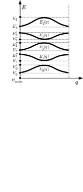
Figure 2.1. Typical dispersion relations

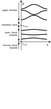
Figure 2.2. Asymptotics of the dispersion relations

There are no explicit analytic formulas expressing the dispersion relations in terms of the potential $v$ even for the simplest potentials (except in the case of finitely many gaps, see [36, Chapter 2], [65, §1.5]). Semiclassical asymptotic formulas are available only for large $E$. We consider now the situation when $h\to+0$ in (2.1). This problem was studied in many papers and monographs, cf. e. g. [62, 42, 33, 35, 56, 79, 92, 91, 48], see also [66] and references there-in, but with a somewhat different point of view. We recall here several results in a form suitable for us, keeping in mind their multidimensional generalization.

2.2. The asymptotics of the spectrum

To simplify the discussion we now assume that $v$ is analytic and has only one non-degenerate minimum point $x_{\text{min}}$ on $S^{1}_{x}$; we may and will assume $v_{\text{min}}:=v(x_{\text{min}})=0$. Then there also exists only one global maximum point $x_{\text{max}}$ of $v$; we put $v_{\text{max}}=v(x_{\text{max}})$. Under this assumption the dispersion picture is divided in four domains. The bands situated under $v_{\text{max}}$ become exponentially small with respect to $h$, and the corresponding dispersion curves are almost horizontal segments $E_{\nu}=\text{const}\mod O(h^{\infty})$ (see Fig. 2.2) with distance $O(h)$ between them; this means that the number of bands increases as $h$ tends to zero, and $\nu$ is allowed to be large. Let $\delta$ denote a small number independent of $h$.

Proposition 2.1.

(a) For $E_{\nu}(q)<v_{\text{max}}-\delta$ we have

(2.4) $$E_{\nu}(q)=E_{1,\nu}+o(h),$$

where $E_{1,\nu}$ is defined by the Bohr-Sommerfeld rule

(2.5) $$\frac{1}{\pi}\int_{x_{-}}^{x_{+}}\sqrt{E_{1,\nu}-v(x)}dx=h(\frac{1}{2}+\nu),$$

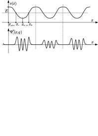
Figure 2.3. Structure of Bloch functions

with $x_{\pm}(E_{1,\nu})$ solutions of the equation $v(x)=E_{1,\nu}$ (see Fig. 2.3).

If $\nu h$ is small enough then $E_{1,\nu}$ is also small and one can simplify (2.5) using a Taylor expansion; this leads to the “harmonic” oscillator approximation for $E_{1,\nu}$,

(2.6) $$E_{1,\nu}=h(\frac{1}{2}+\nu)\omega_{0}+O(h^{2}),\quad\omega_{0}=\sqrt{2v^{\prime\prime}(x_{\text{min}})}.$$

(b) Let $v_{\text{min}}+\delta<E_{1,\nu}<v_{\text{max}}-\delta$, then

(2.7) $$E_{\nu}(q)-E^{-}_{\nu}=\frac{\omega(E_{1,\nu})h}{\pi}((-1)^{\nu+1}\cos(2\pi q)+1)e^{-\rho/h}\bigl{(}1+O(h)\bigr{)}.$$

Here $\omega(E)=2\pi(\int_{x_{-}}^{x_{+}}\frac{1}{\sqrt{E-v(x)}}dx)^{-1}$ is the frequency (see subsection 2.4), and $\rho=\int_{x_{+}}^{x_{-}}\sqrt{v(x)-E_{1,\nu}}dx$ is the Agmon distance [1].

If $\nu h$ is small enough then

(2.8) $$\begin{gathered}E_{\nu}(q)-E^{-}_{\nu}=\frac{2^{4\nu+5/2}{\omega_{0}}^{\nu+3/2}h^{1/2-\nu}}{\nu!\sqrt{\pi}}\times\\ {\exp}{\bigl{(}\frac{1}{4}(2\nu+1)\int_{x_{\text{min}}}^{x_{\text{min}}+2\pi}(\frac{\omega_{0}}{\sqrt{v(x)}}-\frac{1}{\sin{(\frac{x-x_{\text{min}}}{2})}})dx\bigl{)}}\times\\ ((-1)^{\nu+1}\cos(2\pi q)+1)e^{-\rho/h}\bigl{(}1+O(h^{1/2})\bigr{)},\end{gathered}$$

with Agmon distance $\rho=\int_{x_{\text{max}}}^{x_{\text{max}}+2\pi}\sqrt{v(x)-E_{1,\nu}}dx$.

For the proof we refer to [91], see also review of results in [66].

Remarks.

(1) If $\nu\sim 1/h$ then $o(h)$ in (2.4) can be replaced by $O(h^{2})$; the estimate $o(h)$ appears during the passage from “small” to large “large” $\nu$, see [56, 66].

(2) In these asymptotic formulas the potential $v$ appears only through the frequency and the Agmon distance: the dependence on the quasimomentum $q$ is the same for different potentials.

(3) If we formally take the limit $\nu h\to 0$ in (2.7) for ${\nu h}<<1$, we obtain (2.8), but these arguments are not rigorous, so (2.8) has to be proved by other means. In such a situation we say that formula (2.7) allows a formal limit.

(4) The subtraction of $1/\sin{(\frac{x-x_{\text{min}}}{2})}$ from the integrand in (2.8) is just one possible type of regularization.

In the upper domain, on the other hand, the gaps above $v_{\text{max}}$ become exponentially small, the bands have length $O(h)$ and almost cover the spectral half axis.

Proposition 2.2.

For $E_{\nu}(q)>v_{\text{max}}+\delta$ we have $E_{\nu}^{+}-E_{\nu+1}^{-}=O_{\nu}(h^{\infty})$, and the ends of the gaps are defined by a Bohr-Sommerfeld quantization rule in the form

(2.9) $$E_{\nu}^{+}=\mathcal{E}_{\nu}+O_{\nu}(h^{2}),\quad\frac{1}{{2\pi}}\int_{0}^{2\pi}\sqrt{\mathcal{E}_{\nu}-v(x)}dx=\frac{h\nu}{2}.$$

We also have the following asymptotic formulas for the dispersion relation in the $\nu$-th band (Fig .2.2):

(2.10) $$E_{\nu}(q)=E_{2,\nu}(q)+O_{\nu}(h^{2}),\quad\frac{1}{{2\pi}}\int_{0}^{2\pi}\sqrt{E_{2,\nu}(q)-v(x)}dx=I_{\nu}(q,h),$$

where for even $\nu=2s$

(2.11a) $$I_{\nu}(q,h)=\begin{cases}h(\frac{\nu}{2}+q),&0<q<\frac{1}{2},\\ h(\frac{\nu}{2}+1-q),&\frac{1}{2}<q<1,\end{cases}$$

and for odd $$\nu=2s+1$$

(2.11b) $$I_{\nu}(q,h)=\begin{cases}h(\frac{\nu+1}{2}-q),&0<q<\frac{1}{2},\\ h(\frac{\nu-1}{2}+q),&\frac{1}{2}<q<1.\end{cases}$$

For the proof of (2.9), see [35, Appendix B], or [42, §7]. Formulas (2.11a) and (2.11b) in a slightly different form are contained in [30] or [56, Part II].

Remark.

The description of the splitting $E_{\nu+1}^{-}-E_{\nu}^{+}$ between the ends of the gaps is not so simple in this case as in (2.7). In the physics literature, this splitting is associated with the so-called “over barrier” reflection. Under additional assumptions [92, 91, 42, 35], the splitting has the more explicit form:

(2.12) $$E^{-}_{\nu+1}-E_{\nu}^{+}=\frac{\omega(E_{1,\nu})h}{\pi}e^{-\widetilde{\rho}/h}\bigl{(}1+O(h)\bigr{)}.$$

The definition of the Agmon distance $\widetilde{\rho}$, however, is now quite different.

Of course, there is a transient layer in a neighborhood of $v_{\text{max}}$ where the band length is comparable with the gap length; formulas (2.5), (2.7), (2.10), and (2.11) are not valid there. We do not consider this situation (see, nevertheless, [15, 66, 92]).

2.3. Quasimodes and Bloch solutions

The behavior of the Bloch solutions differs sharply in the lower and upper domains. Moreover, it is natural to isolate a certain neighborhood of the bottom of the lower domain, because the behavior of the corresponding eigenfunctions is also different there. The asymptotic formulas depend, of course, on the accuracy of the approximation: they must be more complicated e. g. in case of the subtle dispersion relations (2.8), (2.9).

Recall the following definitions (see e. g. [69, 67, 68, 49, 51, 50, 61]).

Definition 2.1.

Let $L>1$ be a real number.

• A pair $(\Psi^{L},E^{L})$ is called a formal asymptotic solution or quasimode of order $L$, relative to some function space $\mathcal{F}$, if

  (2.13) $$\|(\widehat{L}-E^{L})\Psi^{L}\|_{\mathcal{F}}=O(h^{L}).$$

  We can use, for example, $\mathcal{F}=C(\mathbb{R})$, or $\mathcal{F}=L^{2}(\mathbb{R}_{x})$.

• Let $\Psi$ be a solution of the equation $(\widehat{L}-E)\Psi=0$. The function $\Psi^{L}$ is called an asymptotic part of order $L$ of $\Psi$ if $\|\Psi-\Psi^{L}\|_{\mathcal{F}}=O(h^{L})$ as $h\to 0$.

• Let $\|\Psi^{L}\|\geq c>0$ as $h\to 0$. The function $\Psi^{0}$ is called a leading term of the quasimode $\Psi^{L}$ if $\|\Psi^{L}-\Psi^{0}\|_{\mathcal{F}}=o(1)$ as $h\to 0$.

Remarks.

(1) Note that in the definition of quasimode, the Bloch condition (2.3) is not required.

(2) Definition (2.1) describes so-called “power” or “additive” asymptotics; these notions are used in contrast to “multiplicative” asymptotics, which we will define later.

(3) An asymptotic part contains more information about the true solution of (2.1) than a quasimode, even though both concepts can coincide in specific examples. Nevertheless, one can derive information about the spectrum of $\widehat{L}$ from quasimodes. The following proposition is essentially well known.

Proposition 2.3.

Let $\Psi^{L}$ be a smooth function and $E^{L}\in\mathbb{R}$ with the property

• $(\Psi^{L},E^{L})$ is a quasimode of $\widehat{L}$ of order $L$ in $L^{2}(\mathbb{R})$, and $\|\Psi\|_{L^{2}(\mathbb{R})}\geq c>0$ as $h\to 0$;

• $(\Psi^{L},E^{L})$ is a quasimode of $\widehat{L}$ of order $L$ in $L^{2}[-\pi,\pi]$, $\Psi^{L}$ satisfies (2.3), and $\|\Psi^{L}\|_{L_{2}[-\pi,\pi]}\geq c>0$ as $h\to 0$.

Then the distance between $E^{L}$ and the spectrum of $\widehat{L}$ is $O(h^{L})$.

Proof.

The proof is well known for the case (a), see, for example [67, Lemma 1.3] or [69, Lemma 13.1]. Let us give the proof for the case (b), which is a simple generalization and probably also known.

For any function $\varphi$ satisfying (2.3) we have $\|\varphi\|_{L^{2}[-m\pi,m\pi]}=\sqrt{m}\|\varphi\|_{L^{2}[-\pi,\pi]}$, so this holds, in particular, for $\Psi^{L}$, for $(\Psi^{L})^{\prime}$, and for the discrepancy $f:=(\widehat{L}-E^{L})\Psi^{L}$. Let us choose a smooth cut off function $e$ with $0\leq e\leq 1$, $e(x)=1$ for $x\in(-\pi,\pi)$, and $e(x)=0$ for $x\notin(-2\pi,2\pi)$, and let $|e(x)|+|e^{\prime}(x)|+|e^{\prime\prime}(x)|\leq c_{1}$ for $x\in\mathbb{R}$. For $m\in\mathbb{N}$ we put $e_{m}(x):=e(x/m)$. Since $\widehat{L}$ is self-adjoint, we have

(2.14) $$\|e_{m}\Psi^{L}\|_{L^{2}(\mathbb{R})}\operatorname{dist}(\operatorname{spec}\widehat{L},E^{L})\leq\|(\widehat{L}-E^{L})(e_{m}\Psi^{L})\|_{L^{2}(\mathbb{R})},$$

and the left-hand side satisfies

(2.15) $$\|e_{m}\Psi^{L}\|_{L^{2}(\mathbb{R})}\geq c\sqrt{m},$$

by assumption. To estimate the right-hand side we use

$$(\widehat{L}-E^{L})(e_{m}\Psi^{L})=e_{m}f-h^{2}\frac{d^{2}e_{m}}{dx^{2}}\Psi^{L}-2h^{2}\frac{de_{m}}{dx}\frac{d\Psi^{L}}{dx}.$$

Then

(2.16) $$\|(\widehat{L}-E^{L})(e_{m}\Psi^{L})\|_{L^{2}(\mathbb{R})}\leq\sqrt{2m}\|f\|_{L^{2}[-\pi,\pi]}+\frac{2\sqrt{2}h^{2}c_{1}}{m\sqrt{m}}\|\Psi^{L}\|_{L^{2}[-\pi,\pi]}+\frac{2\sqrt{2}h^{2}c_{1}}{\sqrt{m}}\left\|\frac{d\Psi^{L}}{dx}\right\|_{L^{2}[-\pi,\pi]}.$$

Combining (2.14), (2.15), and (2.16) we obtain in the limit $m\to+\infty$ the desired estimate

$$\operatorname{dist}(\operatorname{spec}\widehat{L},E^{L})\leq\frac{\sqrt{2}}{c}\|(\widehat{L}-E^{L})\Psi^{L}\|_{L^{2}[-\pi,\pi]}=O(h^{L}).$$

∎

To describe the asymptotics of Bloch functions let us start from the simplest level of complexity related to (2.6). One obtains the following picture: Bloch functions associated to the lowest bands are localized in $O(\sqrt{h})$-neighborhoods of the minimum points $x_{\text{min}}+2\pi l$, $l\in\mathbb{Z}$, of the potential $v$, where they coincide to first order with the eigenfunctions of a harmonic oscillator. More precisely, in some $O(\sqrt{h})$-neighborhood of $x_{\text{min}}$ one has the following formula for the leading term in the asymptotics of all Bloch solutions:

(2.17) $$\psi^{\nu}_{0}(x)=C^{\nu}\exp{(-\frac{\omega_{0}(x-x_{\text{min}})^{2}}{4h})}H_{\nu}(\frac{\sqrt{\omega_{0}}(x-x_{\text{min}})}{\sqrt{2h}}),$$

where $C^{\nu}$ is a normalizing constant and $H_{\nu}$ denotes the $\nu$-th Hermite polynomial, whereas the Bloch functions are $O(h^{\infty})$ in all other points of the segment $[x_{\text{max}},x_{\text{max}}+2\pi]$. This together with the Bloch condition completely defines a leading term in suitable neighborhoods of all other minimum points $x_{\text{min}}+2\pi l$, $l\in\mathbb{Z}$, by the formula

(2.18) $$\Psi^{\nu}_{0}(x,q)=\sum_{l\in\mathbb{z}}e^{2\pi iql}\psi^{\nu}_{0}(x-2\pi l).$$

More precisely, for any Bloch function $\Psi^{\nu}$ there exists a function $\psi^{\nu}$ such that

(2.19) $$\Psi^{\nu}(x,q)=\sum_{l=-\infty}^{\infty}e^{2\pi iql}\psi^{\nu}(x-2\pi l);$$

this is the so-called Gelfand representation (see [44, 88], [80, XIII.16]. Let us record the fact that $\psi^{\nu}=\psi^{\nu}_{0}+O(\sqrt{h})$.

Using the terminology introduced above, one can prove that (2.17) gives asymptotics of certain quasimodes of order $L$ for (2.1), and the functions (2.18) are the leading terms of asymptotics of the Bloch solutions. In a way, (2.18) presents the asymptotics of modes via quasimodes, and the approximation (2.17) and (2.18) allow us to derive (2.6). Note that (2.18) gives more information about the Bloch solutions than (2.18) but no better spectral information than (2.6).

The Bloch solutions corresponding to the higher bands are localized in a neighborhood of the segments $[x_{-}+2\pi l,x_{+}+2\pi l]$, $l\in\mathbb{Z}$, where $x_{\pm}$ are solutions of the equation $v(x)=E_{1,\nu}$ introduced above; they can be represented in the form (2.18). This means precisely that in inner points of the interval $(x_{-},x_{+})$ a leading term of all Bloch solutions is given by

(2.20) $$\psi_{0}^{\nu}(x):=\frac{C^{\nu}(h)}{\bigl{(}E_{1,\nu}-v(x)\bigr{)}^{1/4}}\big{(}\cos(\frac{1}{h}\int_{x_{-}}^{x}\sqrt{E_{1,\nu}-v(x)}dx+\frac{\pi}{4})+O(h)\big{)},$$

with $C^{\nu}$ a normalizing constant.

In a neighborhood of the turning points $x_{-}$ and $x_{+}$, the functions $\psi_{0}^{\nu}(x,h)$ are given in terms of Airy functions and have large amplitudes; but they are still $O(h^{\infty})$ outside certain neighborhoods of the segment $[x_{-},x_{+}]$. Thus it follows from (2.18) again that there exist gaps in the asymptotic support of the Bloch solutions (see below for the definition). A global uniform “power” asymptotic of $\psi_{0}^{\nu}$ can be given in terms of Maslov’s canonical operator (we will return to this representation later). Using quasimodes as before, one derives the spectral information given in (2.4) and (2.5).

It is convenient to use some terminology taken from the theory of short-wavelength approximation in optics Let us consider a certain asymptotic solution $\Psi(x,h)$. The closure of the domain where $\lim_{h\to 0}\Psi(x,h)\neq 0$ is called its asymptotic support or light region. The domain where $\Psi(x)=O(h^{\infty})$ as $h\to 0$ is called the shadow region. In some neighborhood of the boundary (this neighborhood is small together with $h$) $\Psi(x,h)$ has order $h^{L}$; sometimes this neighborhood is called the penumbra (this definition, of course, is not rigorous). So for (2.17) (or (2.18)) the light region is the union of the minimum points $x_{\text{min}}+2\pi l$, $l\in\mathbb{Z}$, all other points belong to the shadow region, and the penumbra is some neighborhood of $\{x_{\text{min}}+2\pi l$, $l\in\mathbb{Z}\}$. The light region for the asymptotic solutions related to the higher bands consists of the union of the segments $[x_{-}+2\pi l,x_{+}+2\pi l]$, $l\in\mathbb{Z}$, all other points belong to the shadow region, and the penumbra is the union of certain neighborhoods of the turning points $x_{-}+2\pi l$, $x_{+}+2\pi l$, $l\in\mathbb{Z}$. In quantum mechanics, the shadow region is also sometimes called the under-barrier region.

Now let discuss the representation (2.18) in greater detail.

Proposition 2.4.

We fix $\varepsilon>0$ and denote by $e$ some smooth cut off function with $e(x)=1$ for $x\in(b-\varepsilon,b+2\pi+\varepsilon)$ and $e(x)=0$ for $x\notin(b-2\varepsilon,b+2\pi+2\varepsilon)$ (the number $b$ is defined later).

(a) Let $\nu\in\mathbb{N}$ be a fixed number, then the Bloch function $\Psi^{\nu}$ associated with the $\nu$-th band has the form (2.19), where $\psi^{\nu}(x)$ coincides up to $O(\sqrt{h})$ with the function (2.17) in a certain neighborhood of $x_{\text{min}}$. Outside this neighborhood, in the interval $(b-2\varepsilon,b+2\pi+2\varepsilon)$ we have

(2.21) $$\begin{gathered}\psi^{\nu}(x)=e(x)C^{\nu}\sqrt{\frac{2^{5\nu+1}\omega_{0}^{\nu+1}}{h^{\nu}}}\exp{\big{(}-\frac{1}{h}\Phi(x)\big{)}}\sqrt{\frac{\tan{(\frac{x-x_{\text{min}}}{4})}}{\xi(x)}}\cdot\\ {\exp}{\big{(}\frac{1}{4}(2\nu+1)\int_{x_{\text{min}}}^{x}(\frac{\omega_{0}}{\xi(x)}-\frac{1}{\sin{(\frac{x-x_{\text{min}}}{2})}})dx\big{)}}(\tan{(\frac{x-x_{\text{min}}}{4})})^{\nu}\bigl{(}1+O(h)\bigr{)}.\end{gathered}$$

Here $\Phi(x):=|\int_{x_{\text{min}}}^{x}\sqrt{v(x)}dx|$, $\xi(x)=\Phi^{\prime}(x)=\sqrt{v(x)}$ if $x\geq x_{\text{min}}$ and $\xi(x)=\Phi^{\prime}(x)=-\sqrt{v(x)}$ otherwise. The point $b$ is defined as the unique solution of the equation $\Phi(b)=\Phi(b+2\pi)$, i. e. $\int_{b}^{x_{\text{min}}}\sqrt{v(x)}dx=\int_{x_{\text{min}}}^{b+2\pi}\sqrt{v(x)}dx$.

(b) Let $c_{1}\leq h\nu\leq c_{2}$ for some $c_{1}$, $c_{2}>0$, $\nu\in\mathbb{N}$. Then the Bloch function $\Psi^{\nu}$ associated with the $\nu$th band has the form (2.19), where $\psi^{\nu}(x)$ coincides up to $o(h)$ with (2.20) in the interior of the interval $(x_{-},x_{+})$. Moreover,

(2.22) $$\psi^{\nu}(x)=\begin{cases}C^{\nu}e(x)\dfrac{1}{2(v(x)-E_{1,\nu})^{1/4}}\exp{\left(\frac{1}{h}\int_{x}^{x_{+}}\sqrt{v(x)-E_{1,\nu}}\,dx\right)}\bigl{(}1+O(h)\bigr{)},&x>x_{+}+\varepsilon\\[6.0pt] C^{\nu}e(x)\dfrac{(-1)^{\nu}}{2(v(x)-E_{1,\nu})^{1/4}}\exp{\left(\frac{1}{h}\int_{x_{-}}^{x}\sqrt{v(x)-E_{1,\nu}}\,dx\right)}\bigl{(}1+O(h)\bigr{)},&x<x_{-}-\varepsilon,\\ \end{cases}$$

and $b$ is defined by the equation $\int_{b}^{x_{-}}\sqrt{v(x)-E_{1,\nu}}\,dx=\int_{x_{+}}^{b+2\pi}\sqrt{v(x)-E_{1,\nu}}\,dx$.

The normalizing constants $C^{\nu}$ in (2.21) and (2.22) are the same as in (2.17) and (2.20).

Both asymptotics (2.21) and (2.22) admit differentiation with respect to $x$, i.e. in these formulas $\bigl{(}O(h)\bigr{)}^{\prime}_{x}=O(h)$.

For the proof, we refer to [42, §§ IV.1, IV.4].

Remarks.

(1) Formula (2.21) does not admit a formal limit for $x\to x_{\text{min}}$; in particular, (2.21) contains only the highest degree term $\bigl{(}\sqrt{\omega_{0}/2}(x-x_{\text{min}})\bigr{)}^{\nu}$ of the corresponding Hermite polynomial, but the other terms also play a role in a neighborhood of the minimal points. Of course, it is possible to extend the construction accordingly, but, as we will see below, it is not necessary for obtaining the dispersion relation (2.8). The presence of the $\tan$-like term in (2.21) is only one possible way of regularization; another way of regularization has been used in [48].

(2) One has different constructions for the Bloch functions corresponding to the bottom lower and the inner lower domains. In the first case, they are defined by a real-valued phase and decay exponentially with $h$, while in the second case one needs complex phases, i. e., in this case the Bloch functions have both oscillating and exponentially decaying parts. This phenomenon reflects deep properties of the asymptotics given by Maslov’s canonical operator; this distinction appears more clearly in multidimensional problems.

It is necessary to emphasize that it is not complicated to obtain the asymptotic formulas for the spectrum in this one-dimensional situation, but it is difficult to prove the formulas for the true asymptotics of the Bloch functions. The standard way of doing this in the one-dimensional case is based on WKB methods for ordinary differential equations and matching solutions in the complex plane, see [92, 91, 42, 79, 89]. These methods are applicable in both bottom and inner parts of the lower domain, and allow to obtain also the corresponding dispersion relations. But up to now there is no rigorous generalization of this method to multidimensional problems. On the other hand, there are some methods (see e.g. [67, 68, 1, 33, 48, 49, 51, 50, 84, 85]) which are applicable also to multidimensional spectral problems (like tunneling problems or problems with purely imaginary phase), but they work in the bottom parts of the spectrum only. One may call all these methods “semiclassical approximations” (although not in sense of [60]), because they use certain objects from classical mechanics.

(3) Usually, Bloch functions corresponding to the same band and to the quasimomenta $q$ and $1-q$ are normalized in such a way that their Wronskian is equal to $2i$. This leads to normalizing constants in (2.17) and (2.20) which are exponentially large in $h$. Otherwise, the behavior of the Bloch functions is quite strange: in each segment $[2\pi l,2\pi(l+1)]$ some their linear combination is $O(h^{\infty})$. The appearance of large normalizing constants destroys this effect.

Clearly, the exponential smallness of the lower bands makes it difficult to calculate the spectrum and the Bloch functions numerically.

(4) If for some solution $\Psi$ of (2.1) we have a representation $\Psi=\bigl{(}1+O(h)\bigr{)}\Psi_{0}$ which can be differentiated in $x$, then the function $\Psi_{0}$ is sometimes called a multiplicative asymptotic of $\Psi$; both formulas (2.21), (2.22) together with (2.19) provide examples. In contrast to additive asymptotics, multiplicative asymptotics make sense also in the shadow region. Multiplicative asymptotics are sometimes also called exponential or tunneling asymptotics, because knowing them allows to construct asymptotics of the spectrum with an error $O(e^{-C/h})$ which is necessary to deal with tunneling effects.

Let us show now that from the formulas (2.21) and (2.22) it is easy to derive the dispersion relations (2.7) and (2.9). Of course, this can be done using matching solutions in the complex plane and the one-dimensional WKB method – as mentioned above, – but we give here a derivation based on the simple integral formula suggested by I. M. Lifshits (see [62, §VI.55, Problem 3]).

Recall that if $(\Psi_{1},E_{1})$ and $(\Psi_{2},E_{2})$ are solutions of (2.1) and $\int_{\alpha}^{\beta}\Psi_{1}\Psi_{2}dx\neq 0$, then

(2.23) $$E_{1}-E_{2}=h^{2}\frac{\big{(}{\Psi}_{1}{\Psi^{\prime}}_{2}-{\Psi}_{2}{\Psi^{\prime}}_{1}\big{)}\Big{|}^{\beta}_{\alpha}}{\int_{\alpha}^{\beta}\Psi_{1}\Psi_{2}dx}.$$

Let us choose in (2.23) $\Psi_{i}(x)=\Psi^{\nu}(x,q_{i})$, $E_{i}=E_{\nu}(q_{i})$, $i=1,2$, $\alpha=b$, $\beta=b+2\pi$. Note that both $\Psi_{1}$ and $\Psi_{2}$ are defined by (2.19), and thus we have

$$\big{(}{\Psi}_{1}{\Psi^{\prime}}_{2}-{\Psi}_{2}{\Psi^{\prime}}_{1}\big{)}|^{b+2\pi}_{b}=2\big{(}(\psi^{\nu})^{\prime}(b+2\pi)\psi^{\nu}(b)-\psi^{\nu}(b+2\pi)(\psi^{\nu})^{\prime}(b)\big{)}\bigl{(}\cos(2\pi q_{1})-\cos(2\pi q_{1})\bigr{)},$$

because the supports of the functions $\psi^{\nu}(\cdot-2\pi l)$ do not intersect. In the inner lower domain, for the denominator of (2.23) we have

(2.24) $$\begin{gathered}\int_{b}^{b+2\pi}\Psi_{1}(x)\Psi_{2}(x)\,dx=\sum_{l_{1},l_{2}=-1,0,1}e^{2\pi i(l_{1}q_{1}+l_{2}q_{2})}\int_{b}^{b+2\pi}\psi^{\nu}(x-2\pi l_{1})\psi^{\nu}(x-2\pi l_{2})\,dx\\ {}=\int_{b}^{b+2\pi}\bigl{(}\psi^{\nu}(x)\bigr{)}^{2}dx+O(h^{\infty})=\int_{b}^{b+2\pi}\bigl{(}\psi^{\nu}_{0}(x)\bigr{)}^{2}dx+o(h),\end{gathered}$$

and, therefore,

(2.25) $$\begin{gathered}E_{\nu}(q_{1})-E_{\nu}(q_{2})=2h^{2}\frac{\bigl{(}\psi^{\nu}\bigr{)}^{\prime}(b+2\pi)\psi^{\nu}(b)-\psi^{\nu}(b+2\pi)\bigl{(}\psi^{\nu}\bigr{)}^{\prime}(b)}{\int_{b}^{b+2\pi}(\psi^{\nu}_{0})^{2}dx}\cdot\\ \bigl{(}\cos(2\pi q_{1})-\cos(2\pi q_{2})\bigr{)}\bigl{(}1+o(h)\bigr{)}.\end{gathered}$$

For the ground lower domain we have (2.24) and (2.25) with $o(h)$ replaced by $O(\sqrt{h})$.

To prove (2.7) and (2.8) one has only to substitute (2.21), (2.22) into (2.25).

We observe again that the main term of the dispersion relation is independent of $v$; the potential appears only in its coefficients in terms of higher order in $h$. To determine the nominator in (2.25), one should use a multiplicative asymptotics, while the denominator is defined by power asymptotics.

The Bloch functions for all quasimomenta in the bands from the upper domain are bounded as $h\to 0$ and oscillate everywhere on $\mathbb{R}_{x}$, there are no gaps in their asymptotic support; they can be expressed by means of simple formulas outside neighborhoods of size $O(h^{\infty})$ of the points $q=0,\frac{1}{2}$:

(2.26) $$\Psi(x,q)=C^{\nu,\pm}(q)\left(\frac{\exp\left(\pm\frac{i}{h}\int_{a}^{x}\sqrt{E_{2,\nu}(q,h)-v(x)}dx\right)}{\bigl{(}E_{2,\nu}(q,h)-v(x)\bigr{)}^{1/4}}+O(h)\right).$$

Here $C^{\nu,\pm}(q)$ and $a$ are normalizing constants, $E_{2,\nu}(q)$ is defined by (2.10) and (2.11), and one has to take signs + and – according to $q\in(\frac{1}{2},1)$ and $q\in(0,\frac{1}{2})$, respectively.

The formula (2.26) does not give asymptotics of the solutions of (2.1) in the points $q=0,\frac{1}{2}$, i. e. in the ends of the bands. Due to resonances and tunnel effects between these points, the asymptotics of the true eigenfunctions (the periodic and antiperiodic solutions) are given by the even and odd combinations of the functions (2.26) provided that the constants $C^{\nu}$ and $a$ in (2.26) are chosen appropriately, see [35] for details. In some cases, the constants $C^{\nu,\pm}$ can be expressed through each other; to do this one can normalize the corresponding Bloch function $\Psi^{\nu}(x,q)$ by the condition $\Psi^{\nu}(0,q)=1$ (see [36]).

So for these eigenvalues, (2.26) defines quasimodes but not asymptotics of the modes.

The Bloch functions related to the transient domain are close to the latter ones, but in a neighborhood of the critical points $x_{\text{max}}+2\pi l$, $l\in\mathbb{Z}$, one can express them by means of certain special functions; e. g. if $x_{\text{max}}$ is a non-degenerate critical point of $v$, then these are the Weber (parabolic cylinder) functions.

The results we have mentioned so far are obtained by a variety of techniques but with different levels of complexity. Thus it is considerably more difficult to derive the dispersion relations (2.7) and (2.8) with exponentially small bands — using “multiplicative asymptotics” corresponding to tunnel effects — than (2.4) and (2.6). The analysis of the transient domain — which we have not explained here — becomes even more complicated.

Some of the methods mentioned above have been extended to problems in higher dimensions but not in a systematic way. For such an approach, from the general philosophy of quantum mechanics we should expect a correspondence between certain characteristic parts of the spectrum of $\widehat{L}$ (so-called spectral series) and certain characteristic geometric objects in the phase space of the classical motion. In our one-dimensional example, the classical motion is integrable, such that inspiration gained here can be expected to extend at least to the generic integrable case, and that is what we want to explain.

In the case at hand, the spectrum of $\widehat{L}$ may be decomposed into four domains having similar asymptotic behavior as detailed above; these are spectral series. We are now going to show that the presence of different types of asymptotics naturally corresponds to a decomposition of the phase space into “regimes” which each allow a simultaneous treatment of the flow. This decomposition, in turn, is characterized by a single graph which, in this example, coincides with the Reeb graph of the corresponding classical Hamiltonian.

2.4. The graph of the classical motion

We now want to construct classical preimages of the spectral series described above. To do so, we give a suitable classification of the classical motion and establish a relationship with the “quantum motion” defined by (2.1). Thus we have to consider the corresponding classical problem defined by the one-dimensional Hamiltonian

(2.27) $$H(p,x):=p^{2}+v(x).$$

The related Hamiltonian system

(2.28) $$\left.\begin{aligned} \dot{p}&=-v^{\prime}(x)\\ \dot{x}&=2p\end{aligned}\right\}\quad\Longleftrightarrow\quad\ddot{x}=-2v^{\prime}(x),$$

can be considered from two points of view: (1) as a system with phase space $\mathbb{R}_{p,x}^{2}$; (2) as a system with phase space the cylinder $Q^{2}_{p,x}:=\mathbb{R}_{p}\times S^{1}_{x}$, such that $\mathbb{R}^{2}_{p,x}$ is the universal covering of $Q^{2}_{p,x}$.

Then we can distinguish the following types of the trajectories:

1. closed trajectories on $\mathbb{R}^{2}_{p,x}$ which correspond to closed contractible trajectories on $Q^{2}_{p,x}$ (on these we have $v_{\text{min}}<H<v_{\text{max}}$);

2. open trajectories on $\mathbb{R}^{2}_{p,x}$ which correspond to closed but not contractible trajectories on $Q^{2}_{p,x}$ (on these we have $H>v_{\text{max}}$);

3. the stable minimum points $(0,x_{\text{min}}+2\pi l)$ on $\mathbb{R}^{2}_{p,x}$ or on $Q^{2}_{p,x}$;

4. the saddle points $(0,x_{\text{max}}+2\pi l)$ on $\mathbb{R}^{2}_{p,x}$ or on $Q^{2}_{p,x}$ and the singular manifolds (separatrices) on $\mathbb{R}^{2}_{p,x}$ or $Q^{2}_{p,x}$, which belong to the “singular” energy level $v_{\text{max}}$.

This correspondence can be easily illustrated if one imagines that the trajectories of the Hamiltonian system are level curves of the height function of the deformed cylinder, see Fig. 2.4.

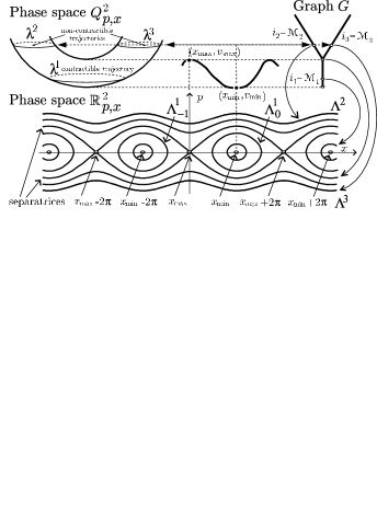
Figure 2.4. Reeb graph and trajectories of Hamiltonian system

Both phase pictures decompose qualitatively into the stationary point(s), the separatrix, and the three connected components of the complement of their union; obviously, two of the three components are equivalent under the map $p\mapsto-p$. Relating this to the energy function, we see that the stationary point(s) correspond(s) to $v_{\text{min}}$ while the separatrix corresponds to $v_{\text{max}}$. Hence the Reeb graph $G$ [19] of $H$ describes the situation nicely, cf. Fig. 2.4. The Reeb graph is constructed as follows: each connected component of the level set of $H$ corresponds to a point of this graph, and connectivity in this set is introduced in a natural way. In our case, the Reeb graph has four vertices, $v_{\text{min}}$, $v_{\text{max}}$, and $\infty_{2/3}$, and edges $i_{1}:=(v_{\text{min}},v_{\text{max}})$, $i_{2/3}:=(v_{\text{max}},\infty_{2/3})$. Moreover, each edge may be identified with an interval of the energy axis. We observe next that for each edge of the graph we have to introduce a different action variable which we denote by $I^{r}$, where $r=1,2,3$ numbers the corresponding edge. For the edge $i_{1}$ we have

(2.29) $$I^{1}(H)=\frac{1}{{2\pi}}\oint_{\Lambda^{1}_{l}}pdx=\frac{1}{\pi}\int_{x_{-}}^{x_{+}}\sqrt{H-v(x)}dx,\quad H<v_{\text{max}}.$$

For $i_{2/3}$ we have:

(2.30) $$I^{2/3}(H)=\frac{1}{2\pi}\int_{0}^{2\pi}\sqrt{H-v(x)}dx,\quad H>v_{\text{max}}.$$

Introduce the action variable in the saddle points:

$$I^{1+}(v_{\text{max}}) =\lim_{H\to v_{\text{max}}-0}I^{1}(H)=\frac{1}{{\pi}}\int_{0}^{2\pi}\sqrt{v_{\text{max}}-v(x)}dx,$$

$$I^{2-/3-}(v_{\text{max}}) =\lim_{H\to v_{\text{max}}+0}I^{2/3}(H)=\frac{1}{2\pi}\int_{0}^{2\pi}\sqrt{v_{\text{max}}-v(x)}dx.$$

Obviously, $\lim_{H\to v_{\text{max}}+0}I^{1}(H)=0$, and $\lim_{H\to+\infty}I^{2/3}(H)=+\infty$, so $I^{1}\in[0,I^{1+}(v_{\text{max}})]$ and $I^{2/3}\in[I^{2+/3+},+\infty)$. One has the “Kirchoff law” $I^{1+}(v_{\text{max}})=I^{2-}(v_{\text{max}})+I^{3-}(v_{\text{max}})$, such that $I^{1+}(v_{\text{max}})=2I^{2-/3-}(v_{\text{max}})$.

Since the functions $I^{r}$ are continuous and strictly increasing, we can invert them to find the dependence of $H$ on $I$ for each edge,

(2.31) $$H=\mathcal{H}^{r}(I),$$

where $\mathcal{H}^{2}(I)=\mathcal{H}^{3}(I)$. Next we will also parameterize the trajectories by the action variables, separately for each edge $i_{r}$, $r=1,2,3$.

We have obtained three open subsets in the phase space $\mathbb{R}^{2}$ corresponding to the edges $i_{r}$ to be denoted by $\mathcal{M}_{r}$, $r=1,2,3$; these are the regimes mentioned above.

In $\mathcal{M}_{1}$, we have only closed trajectories grouped together by their images in $Q^{2}$. These curves can be parameterized by the action variable as follows:

$$\Lambda^{1}_{l}(I)=\bigl{(}p_{1l}(I,t),x_{1l}(I,t)\bigr{)},\quad I\in(0,I^{1+}),\,t\in[0,T(I)],\,l\in\mathbb{Z},$$

where $\bigl{(}p_{1l}(I,t),x_{1l}(I,t)\bigr{)}$ is the solution of (2.28) satisfying

$$p_{1l}(I,0)=0,\quad x_{10}(I,0)=x_{-}\bigl{(}\mathcal{H}^{1}(I)\bigr{)},$$

and

$$x_{1l}(I,0)=x_{10}(I,0)+2\pi l.$$

Thus all the trajectories $\Lambda^{1}_{l}$ are uniquely determined and periodic with period

$$T(I)=\int_{x_{-}\bigl{(}\mathcal{H}^{1}(I)\bigr{)}}^{x_{+}\bigl{(}\mathcal{H}^{1}(I)\bigr{)}}\frac{1}{\sqrt{\mathcal{H}^{1}(I)-v(x)}}\,dx;$$

all $\Lambda^{1}_{l}$ cover the same trajectory $\lambda^{1}$ on $Q^{2}$.

In $\mathcal{M}_{2}$ (and likewise in $\mathcal{M}_{3}$) we obtain quite similarly families of trajectories

$$\Lambda^{2}(I)=\bigl{(}p_{2}(I,t),x_{2}(I,t)\bigr{)},\quad I\in(I^{2-},\infty),\,t\in\mathbb{R},$$

where $\bigl{(}p_{2}(I,t),x_{2}(I,t)\bigr{)}$ is the solution of (2.28) satisfying

$$p_{2/3}(I,0)=\pm\sqrt{\mathcal{H}^{2/3}(I)-v_{\text{max}}},\quad x_{2/3}(I,0)=x_{\text{max}}.$$

$\Lambda^{2/3}$ covers a unique trajectory, $\lambda^{2/3}$, on $Q^{2}$ and enjoys the periodicity property

$$p_{2/3}\bigl{(}I,t+T(I)\bigr{)}=p_{2/3}\bigl{(}I,t\bigr{)},\quad x_{2/3}\bigl{(}I,t+T(I)\bigr{)}=x_{2/3}\bigl{(}I,t\bigr{)}\pm 2\pi,$$

where now

$$T(I)=\frac{1}{2}\int_{-\pi}^{\pi}\frac{1}{\sqrt{\mathcal{H}^{2/3}(I)-v(x)}}\,dx.$$

All the trajectories $\Lambda^{1}_{l}$, $\Lambda^{2/3}$ are one-dimensional Lagrangian manifolds. The closed curves $\Lambda^{1}_{l}$ have a Maslov index equal to $2$; the curves $\Lambda^{2/3}$ are open and their Maslov index is not defined.

Finally, we see that the phase space is separated into regimes corresponding to edges of the Reeb graph for $H$. Trajectories from the same regime have similar topological characteristics. Singular manifolds form the boundaries of the regimes.

Of course, for a general potential $v$ (even required to be a Morse function) the Reeb graph can become very complicated. It is impossible to give a “generic” description of the Reeb graph because there exists no “generic” potential. But obviously the procedure described above is applicable in any case.

2.5. The relationship between the graph and spectral asymptotics

Now it is quite easy to see that our regimes are suitable objects for semiclassical quantization or, more precisely, that they explain the spectral series of the Sturm-Liouville problem (2.1) as described in 2.2 above, corresponding to the four energy domains. Indeed, we set up the following relationship (Fig. 2.6):

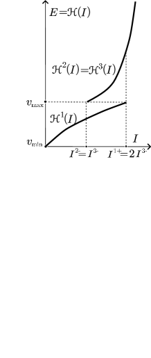
Figure 2.5. Dependence of the energy on the action

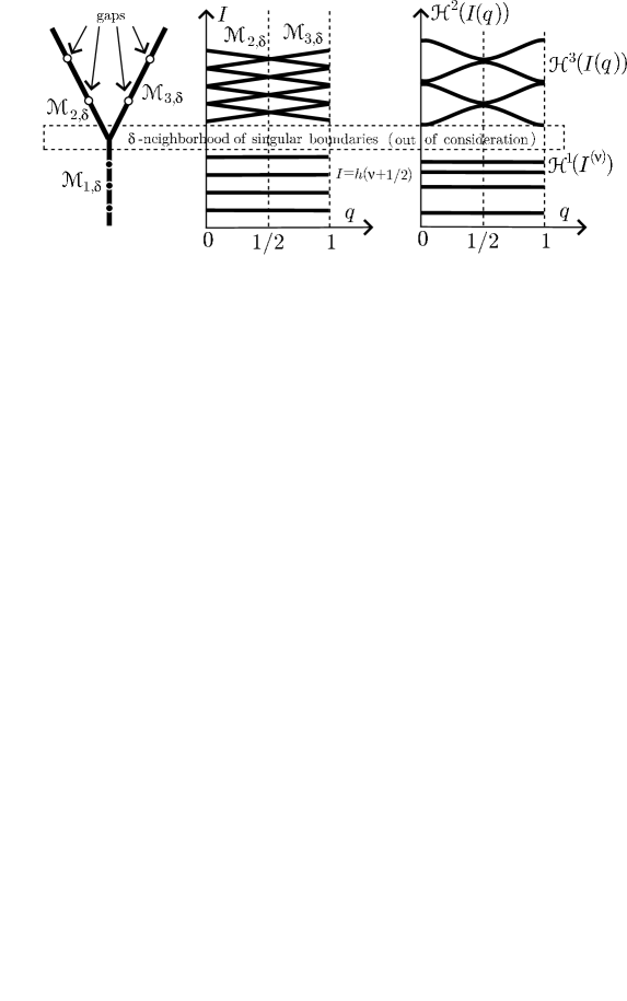
Figure 2.6. Relationship between the Reeb graph and spectral series

bottom lower domain $\longleftrightarrow$	bottom part of the regime $\mathcal{M}_{1}$;
inner lower domain $\longleftrightarrow$	inner part of the regime $\mathcal{M}_{1}$;
“transient” layer $\longleftrightarrow$	some small neighborhood of the boundary between $\mathcal{M}_{1}$, and $\mathcal{M}_{2/3}$;
upper domain $\longleftrightarrow$	the regimes $\mathcal{M}_{2}$ and $\mathcal{M}_{3}$.

Keeping in mind the previous explanation concerning the “transient” layer let us introduce new regimes $\mathcal{M}_{1,\delta}$, $\mathcal{M}_{r,\delta}$, $r=2,3$ which are the “old” regimes but without certain $\delta$-neighborhoods of the singular points $I=I^{1+}$, $I=I^{2-/3-}$; we will describe the semiclassical quantization in these domains.

Consider first the regime $\mathcal{M}_{1,\delta}$ (related to the edge $i_{1}$). The Bohr-Sommerfeld rule (2.5) in this situation may be rewritten in the form

(2.32) $$I=I^{(\nu)}\equiv h\Big{(}\frac{1}{2}+\nu\Big{)}$$

and gives the “quantized regime” or the spectral series corresponding the the regime $\mathcal{M}_{1,\delta}$ (or to the edge $i_{1}$). The non-negative integers $\nu$ are chosen in such a way that $I^{(\nu)}\in[0,I^{1+}-\delta]$. Hence $\nu\sim 1/h$ if $I>\delta>0$. The map (2.31) together with the closed curves $\Lambda^{1}_{l}(I^{(\nu)})$ gives the set $E_{1,\nu}=\mathcal{H}^{r}(I^{(\nu)})$ of “asymptotic” eigenvalues (2.5) and the quasimodes for the operator $\widehat{L}$; in fact, one can prove that for each $L,l\in\mathbb{N}$ one can find the numbers (independent of $l$)

(2.33) $$E^{L}_{1,\nu}=E_{1,\nu}+O(h^{2})$$

and a family of quasimodes $\psi_{l}^{\nu,L}(x,h)$ of (2.1) of order $L$ such that

(2.34) $$\operatorname{supp}_{h\to 0}\psi_{l}^{\nu,L}(x)\to\pi_{x}\Lambda^{1}_{l},$$

where $\pi_{x}$ denotes the projection onto the $x$-plane. This general construction is well known (see e.g. [42, 69, 56]) and may be carried out using Maslov’s canonical operator $\mathcal{K}_{\Lambda^{1}_{l}(I^{(\nu)})}$ on the curve $\Lambda^{1}_{l}(I^{(\nu)})$ (for $I^{(\nu)}>\kappa>0$ one can use the real canonical operator, in case $I^{(\nu)}\to 0$ it is necessary to use the complex canonical operator). For the leading term one has

(2.35) $$\psi_{l}^{\nu}(x,h)=\mathcal{K}_{\Lambda^{1}_{l}(I^{(\nu)})}\cdot 1.$$

If $I^{(\nu)}$ is small, then the last formula for $l=0$ is (2.17). If $I^{(\nu)}>\kappa>0$, then outside some small neighborhood of the intervals $[x_{-}+2\pi l,x_{+}+2\pi l]=\pi_{x}\Lambda^{1}_{l}(I^{(\nu)})$ we have $\psi_{l}^{\nu}(x,h)=O(h^{\infty})$, and for $\psi_{0}^{\nu}(x,h)$ one has formula (2.19) in the inner points of the interval $(x_{-},x_{+})$.

One may also express $\psi_{l}^{\nu}(x,h)$ via $\psi_{0}^{\nu}(x,h)$ by the formula

(2.36) $$\psi_{l}^{\nu}(x,h)=\psi_{0}^{\nu}(x-2\pi l,h).$$

Now let us return to quasimodes and the Bloch conditions (2.3). We know that (2.18) holds in the case at hand, but its proof uses additional nontrivial asymptotic considerations, and some of them are not yet available in multidimensional situations. But let us give some simple heuristic and purely algebraic argument how to obtain (2.18) with the ansatz

(2.37) $$\Psi^{\nu}_{0}(x,q,h)=\sum_{l=-\infty}^{\infty}C_{l}(q,h)\psi^{\nu}_{0}(x-2\pi l,h),\quad$$

where $C_{l}(q,h)$ are unknown coefficients. Requiring the Bloch condition we find

$$\sum_{l=-\infty}^{\infty}C_{l}(q)\psi^{\nu}_{0}(x-2\pi(l-1),h)=e^{2\pi iq}\sum_{l=-\infty}^{\infty}C_{l}(q)\psi^{\nu}_{0}(x-2\pi l,h).$$

If the system $\bigl{(}\psi^{\nu}_{0}(x-2\pi l,h)\bigr{)}_{l\in\mathbb{Z}}$ has suitable basis properties, we conclude

(2.38) $$C_{l+1}(q)=C_{l}(q)e^{2\pi iq},$$

hence $C_{l}=e^{2\pi iql}C^{\nu}$, where $C^{\nu}$ is a normalizing constant and $q\in[0,1)$, and we obtain formulas (2.18), (2.19), and as corollary the structure of the dispersion relation (2.25). This consideration does not depend on $L$, the degree of approximation.

So in this case the used semiclassical method gives a $O(h^{\infty})$-approximation of the dispersion relations and the asymptotics for the Bloch functions.

Now consider the regimes $\mathcal{M}_{r,\delta}$ corresponding to the edges $i_{r}$, $r=2,3$. There are no cycles on $\Lambda^{2,3}(I)$, and for each $I\in\mathcal{M}_{r,\delta}$ and arbitrary large $L$ one can write the following formula for the asymptotic solutions:

(2.39) $$\psi^{\pm}(x,h,E)=C^{\pm}\left(\frac{\exp\left(\pm\frac{i}{h}\int_{a}^{x}\sqrt{E-v(x)}dx\right)}{\bigl{(}E-v(x)\bigr{)}^{1/4}}+O(h)\right),\quad E>v_{\text{max}}+\delta,$$

where the sign + corresponds to $\mathcal{M}_{2}$, the sign – to $\mathcal{M}_{3}$, and $a$ and $C^{\pm}$ are some constants. The function $\psi^{\pm}$ is associated with the spectral value

(2.40) $$E^{L}(I,h)=\mathcal{H}^{2}(I)+O(h^{2})=\mathcal{H}^{3}(I)+O(h^{2}).$$

Requiring now the Bloch condition for the functions $\psi^{\pm}$, we derive the dependence of $I$ on $q$ as

(2.41) $$I^{2}(q,h)=h(n+q),\quad I^{3}(q,h)=h(n-q),\quad n\in\mathbb{Z}.$$

This dependence also implies the dependence of the energy on the quasimomenta,

(2.42) $$E^{2/3,L}(q)=E^{L}\bigl{(}I^{2/3}(q,h),h\bigr{)}.$$

Recall that the points of the spectrum corresponding to periodic and anti-periodic solutions of (2.1) lie on the ends of the bands. Applying this fact to the function (2.39) one immediately obtains the points

(2.43) $$I^{(\nu)}=h\nu/2,\quad\nu\in\mathbb{Z}$$

from $\mathcal{M}_{r,\delta}$, $r=2,3$; the corresponding energy levels $E^{L}\bigl{(}I^{(\nu)}\bigr{)}$ are therefore $O(h^{\infty})$-approximations of the gaps.

Combining now (2.41), (2.42), and (2.43), we arrive at the dispersion relations (2.10)–(2.12).

Note that points (2.43) with even $\nu$ may be obtained by means of the Bohr-Sommerfeld quantization of the non-contractible closed preimages of ${\Lambda}^{2,3}(I)$ on the cylinder $Q^{2}_{p,x}$. This fact has a rather simple explanation: these points correspond to periodic solutions of (2.1), and only these Bloch solutions descend to functions on the cylinder $Q^{2}_{p,x}$. Anti-periodic solutions do not descend to functions on $Q^{2}_{p,x}$, but only to the enlarged cylinder $\widetilde{Q}^{2}_{p,x}=\mathbb{R}_{p}\times S^{1}_{x}$, $x\in[0,4\pi)$. The Bohr-Sommerfeld quantization rule on $\widetilde{Q}^{2}_{p,x}$ then gives exactly the points (2.43).

Figure 2.6 shows the relationship between action variables, quasimomenta and energy. This picture together with formulas (2.4)–(2.6), (2.9)–(2.11), (2.18), (2.25) contains the maximal information about the spectrum of $\widehat{L}$ which can be derived from additive asymptotics.

The precise structure of the dispersion relations is sketched in Fig. 2.7; it is not accessible in details by these methods.

Figure 2.7. Exact dispersion relations

2.6. The Weil formula

To conclude this section, let us suggest a heuristic method for calculating the number $N(E)$ of bands on the half-line $(-\infty,E)$ (the Weyl formula).

If $E\leq v_{\text{min}}$, there are no real trajectories of the Hamiltonian $H(p,x)$, no points on the graph $G$ and $N(E)=0$.

If $E\in(v_{\text{min}},v_{\text{max}}-\delta)$, then the number of bands approximately coincides with the number of the Bohr-Sommerfeld points $I_{\nu}$ (2.32) in the interval $(v_{\text{min}},E)$, i.e. with $I(E)/h$.

If $E\geq v_{\text{max}}+\delta$, then we have gaps on the edges $i_{2}$ and $i_{3}$, but by symmetry their projections to the energy axis coincide and one has to take into account only one edge, say $i_{2}$, which gives $N(E)=I^{1+}/h+2\bigl{(}I(E)-I^{2-}\bigr{)}/h=2I(E)/h$.

Last two formulas have common geometric interpretation: $hN(E)$ is approximately equal to the square of the set $0\leq x\leq 2\pi$, $H(p,x)\leq E$, i.e. the set covered by the trajectories of (2.28) with energy not greater than $E$.

3. Classical averaging

Now we return to the spectral problem of the magnetic Schrödinger operator (1.1). We will use ideas closed to those collected in the previous section, but we will start directly with the classical problem. First we want to show that the presence of the small parameter $\varepsilon$ renders the almost integrable system. Basing on this fact, we give a global geometric classification of the classical motion in the following sections.

Consider the classical problem in the phase space $\mathbb{R}^{4}_{p,x}$ induced by the operator $\widehat{H}$ and defined by the Hamiltonian (1.7):

(3.1) $$H=H_{0}+\varepsilon v(x_{1},x_{2}),\qquad H_{0}=\frac{1}{2}(p_{1}+x_{2})^{2}+\frac{1}{2}p^{2}_{2}.$$

The projections of the trajectories of the Hamiltonian system with free Hamiltonian $H_{0}$ onto the $(x_{1},x_{2})$-plane are the cyclotron circles, see e.g. [2, 78, 16, 18, 63], and they induce new canonical variables in the phase space: generalized momenta $I_{1}$, $y_{1}$ (or $P$, $y_{1}$) and generalized positions $\varphi_{1}$, $y_{2}$ or ($Q$, $y_{2}$):

(3.2) $$\begin{gathered}x_{1}=Q+y_{1},\quad p_{1}=-y_{2},\quad x_{2}=P+y_{2},\quad p_{2}=-Q,\\ P=\sqrt{2I_{1}}\cos\varphi_{1},\quad Q=\sqrt{2I_{1}}\sin\varphi_{1},\end{gathered}$$

such that

$$dp_{1}\wedge dx_{1}+dp_{2}\wedge dx_{2}=dI_{1}\wedge d\varphi_{1}+dy_{1}\wedge dy_{2}=dP\wedge dQ+dy_{1}\wedge dy_{2}.$$

The variables $P$, $Q$ (or $I_{1}$, $\varphi$) describe fast rotating motion around slow guiding center with coordinates $y_{1}$, $y_{2}$ [63].

In these variables, the Hamiltonian $H$ takes the form

(3.3) $$H=I_{1}+\varepsilon v(\sqrt{2I_{1}}\sin\varphi_{1}+y_{1},\sqrt{2I_{1}}\cos\varphi_{1}+y_{2}),$$

and furnishes probably the simplest example where the averaging methods (see e.g.[4, 17, 16, 71]) can be successfully applied. The averaging procedure for the Hamiltonian $H$ was first applied by van Alfven [2]; later, it was used in numerous works (usually, not in the variables $(I_{1},\varphi_{1},y)$, $y=(y_{1},y_{2})$, see e.g. [3, 16, 17, 18, 63, 70, 78]). Our goal here is to obtain some elementary formulas for the averaged Hamiltonian, which are probably new, and to give a global interpretation of the averaged motion basing on the geometrical and topological approaches to integrable Hamiltonian systems developed in [19, 20, 43]. We are also going to show that general result [71] gives probably the most complete statement about the averaging for $H$; it seems that the variables $(I_{1},\varphi_{1},y)$ are most convenient for the analysis involved

To simplify further formulas, let us introduce the averaged potential $\bar{v}$. Expand $v$ into the Fourier series:

(3.4) $$v(x_{1},x_{2}) =v(Q+y_{1},P+y_{2})$$

$$=v(\sqrt{2I_{1}}\sin\varphi_{1}+y_{1},\sqrt{2I_{1}}\cos\varphi_{1}+y_{2})$$

$$=\sum_{k=(k_{1},k_{2})\in\mathbb{Z}^{2}}v_{k}\exp\bigg{[}i\Big{(}k_{1}\big{(}\sqrt{2I_{1}}\sin\varphi_{1}+y_{1}-\frac{2\pi a_{21}}{a_{22}}(\sqrt{2I_{1}}\cos\varphi_{1}+y_{2})\big{)}$$

$$\quad\quad+k_{2}\frac{2\pi}{a_{22}}\big{(}\sqrt{2I_{1}}\cos\varphi_{1}+y_{2}\big{)}\Big{)}\bigg{]}.$$

Now let us average the potential $v$ with respect to the angle variable $\varphi_{1}$:

(3.5) $$\bar{v}(I_{1},y_{1},y_{2})=\frac{1}{2\pi}\int_{0}^{2\pi}v\,d\varphi_{1}.$$

Taking into account expansion (3.4) and using Bessel’s integral representation for the Bessel functions [52, no. 7.3.1], one can rewrite (3.5) as

(3.6) $$\bar{v}(I_{1},y_{1},y_{2}) =\sum_{k=(k_{1},k_{2})\in\mathbb{Z}^{2}}v_{k}J_{0}(\sqrt{2I_{1}(k^{2}_{1}+(2\pi)^{2}(k_{2}-k_{1}a_{21})^{2}/a^{2}_{22})}$$

$$\quad\quad\times\exp\left[ik_{1}\Big{(}y_{1}-\frac{2\pi a_{21}}{a_{22}}y_{2}\Big{)}+ik_{2}\frac{2\pi y_{2}}{a_{22}}\right],$$

where $J_{0}$ is the Bessel function of order zero. Using the spectral theorem, (3.6) can be rewritten in a more elegant form:

$$\bar{v}(I_{1},y_{1},y_{2})=J_{0}(\sqrt{-2I_{1}\Delta})v(y_{1},y_{2}).$$

Here the operator $J_{0}(\sqrt{-2I_{1}\Delta})$ is a pseudo-differential operator [82]. Note that $\bar{v}$ is analytical with respect to $I_{1}$, because $J_{0}$ is an even function.

Let us formulate now our main result on averaging.

Theorem 3.1.

For any $\kappa>0$ there exist $\varepsilon_{0}>0$, positive constants $C$ and $G$, and a canonical change of variables

$$P =\mathcal{P}+\varepsilon U_{1}(\mathcal{P},\mathcal{Q},\mathcal{Y}_{1},\mathcal{Y}_{2},\varepsilon), \quad Q =\mathcal{Q}+\varepsilon U_{2}(\mathcal{P},\mathcal{Q},\mathcal{Y}_{1},\mathcal{Y}_{2},\varepsilon),$$

$$y_{1} =\mathcal{Y}_{1}+\varepsilon W_{1}(\mathcal{P},\mathcal{Q},\mathcal{Y}_{1},\mathcal{Y}_{2},\varepsilon), \quad y_{2} =\mathcal{Y}_{2}+\varepsilon W_{2}(\mathcal{P},\mathcal{Q},\mathcal{Y}_{1},\mathcal{Y}_{2},\varepsilon),$$

defined in the domain $\mathcal{I}_{1}<\kappa$, $\varepsilon<\varepsilon_{0}$ (here and later $\mathcal{I}_{1}=\frac{1}{2}(\mathcal{P}^{2}+\mathcal{Q}^{2})$), such that

$$H=\mathcal{H}(\mathcal{I}_{1},\mathcal{Y},\varepsilon)+e^{-C/\varepsilon}\mathcal{G}(\mathcal{P},\mathcal{Q},\mathcal{Y},\varepsilon).$$

Here $U_{1,2}$, $W_{1,2}$, $\mathcal{G}$ are real analytic functions of $\mathcal{P}$, $\mathcal{Q}$, $\mathcal{Y}$, and

$$|U_{1,2}|,|W_{1,2}|,|\mathcal{G}|+|\nabla_{\mathcal{Y}}\mathcal{G}|\leq G,$$

$\mathcal{H}$ is a real analytic function of $\mathcal{I}_{1}$ and $\mathcal{Y}$. The functions $U_{1,2}$, $W_{1,2}$, $\mathcal{G}$, $\mathcal{H}$ are periodic relative $\mathcal{Y}$ with periods $(a_{1},a_{2})$. In addition, we have the estimate

$$\mathcal{H}(\mathcal{I}_{1},\mathcal{Y},\varepsilon)=\bar{H}(\mathcal{I}_{1},\mathcal{Y},\varepsilon)+\varepsilon^{2}g(\mathcal{P},\mathcal{Q},\mathcal{Y},\varepsilon),\quad\bar{H}(\mathcal{I}_{1},\mathcal{Y},\varepsilon)=\mathcal{I}_{1}+\varepsilon\bar{v}(\mathcal{I}_{1},\mathcal{Y}),$$

where $|g|+|\nabla_{\mathcal{Y}}g|\leq M$ for some positive constant $M$ independent of $\varepsilon$.

Proof of the theorem follows immediately from the general result of Neishtadt [71] in the domain $\mathcal{I}_{1}>\kappa_{0}>0$. To include in our consideration the neighborhood of $I_{1}=0$, we need some its modification based on some special choice of generating function of the requested transformation. On the first step, one has to find a canonical change of variables $(P,Q,y)\mapsto(P^{\prime},Q^{\prime},y^{\prime})$ that reduces the Hamiltonian to the form

(3.7) $$H=H^{\prime}(I_{1}^{\prime},y^{\prime},\varepsilon)+\varepsilon^{2}g(P^{\prime},Q^{\prime},y^{\prime},\varepsilon),$$

where $I^{\prime}_{1}=\bigl{(}(P^{\prime})^{2})+(Q^{\prime})^{2}\bigr{)}/2$, and $g=O(1)$ as $\varepsilon$ tends to $0$. Let us try to find this change of variables using generating function $S(P^{\prime},Q,y^{\prime}_{1},y_{2})=P^{\prime}Q+y^{\prime}_{1}y_{2}+\varepsilon s(P^{\prime},Q,y^{\prime}_{1},y_{2})$ from the equations

(3.8) $$P=P^{\prime}+\varepsilon\frac{\partial s}{\partial Q},\quad Q^{\prime}=Q+\varepsilon\frac{\partial s}{\partial P^{\prime}},\quad y_{1}=y^{\prime}_{1}+\varepsilon\frac{\partial s}{\partial y_{2}},\quad y^{\prime}_{2}=y_{2}+\varepsilon\frac{\partial s}{\partial y^{\prime}_{1}}.$$

Substituting (3.8) into (3.7), one obtains the following condition on $s$:

(3.9) $$Q\frac{\partial s}{\partial P^{\prime}}-P^{\prime}\frac{\partial s}{\partial Q}=\widetilde{v}(P^{\prime},Q,y^{\prime}_{1},y_{2}),$$

where

$$\widetilde{v}(P^{\prime},Q,y^{\prime}_{1},y_{2})=\bar{v}\Big{(}\frac{1}{2}\bigl{(}(P^{\prime})^{2}+Q^{2}\bigr{)},y^{\prime}_{1},y_{2}\Big{)}-v(Q+y^{\prime}_{1},P^{\prime}+y_{2}).$$

Introducing polar coordinates $I,\psi$ by the equalities $P^{\prime}=\sqrt{2I}\cos\psi$, $Q=\sqrt{2I}\sin\psi$, one can rewrite (3.9) in the form $s^{\prime}_{\psi}=\widetilde{v}$. General solution of this equation can be written as $s=\int\widetilde{v}\,d\psi$, but the function $s$ can be non-analytical relative $P^{\prime}$ and $Q$; to avoid this, one should choose the integration constant in a special way, for example,

$$s(P^{\prime},Q,y^{\prime}_{1},y_{2})=\frac{1}{2}\bigg{(}\int_{0}^{\psi}\widetilde{v}(\sqrt{2I}\cos\varphi,\sqrt{2I}\sin\varphi,y^{\prime}_{1},y_{2})\,d\varphi\\ {}+\int_{\pi}^{\psi}\widetilde{v}(\sqrt{2I}\cos\varphi,\sqrt{2I}\sin\varphi,y^{\prime}_{1},y_{2})\,d\varphi\bigg{)}\Bigg{|}_{\begin{subarray}{c}P^{\prime}=\sqrt{2I}\cos\psi,\\ Q=\sqrt{2I}\sin\psi\end{subarray}}.$$

This procedure is then repeated, and the Neishtadt estimations [71] are used, see [24] or [45] for details. Note that on the first step described above one has $H^{\prime}=I^{\prime}_{1}+\varepsilon\bar{v}(I^{\prime}_{1},y^{\prime})$.

We illustrate the above consideration in the special case of example (1.9). Then we find

(3.10) $$\bar{v}(I_{1},y)=AJ_{0}(\sqrt{2I_{1}})\cos y_{1}+BJ_{0}(\beta\sqrt{2I_{1}})\cos(\beta y_{2}).$$

Properties of the Bessel functions [52, no. 7.4] give the estimations

$$\bar{v}(I_{1},y) =A(1-\frac{1}{2}I_{1})\cos y_{1}+B(1-\frac{1}{2}\beta^{2}I_{1})\cos(\beta y_{2})+O(I_{1}^{2}), \quad\text{as }I_{1}\to+0,$$

$$\bar{v}(I_{1},y) =A\sqrt{\frac{2}{\pi\sqrt{2I_{1}}}}\cos(\sqrt{2I_{1}}-\pi/4)\cos y_{1}$$

$$\quad{}+\frac{B}{\sqrt{\beta}}\cos(\beta\sqrt{2I_{1}}-\pi/4)\cos(\beta y_{2})+O(I_{1}^{-3/4}), \quad\text{as }I_{1}\to\infty.$$

4. Classification of the averaged motions

4.1. A one-dimensional Hamiltonian system for the drift

Since the function $\mathcal{H}$ is a periodic function of $\mathcal{Y}$, it can be viewed as defining a Hamiltonian system in two different phase spaces, namely:

• in Euclidean phase space $\Phi=\mathbb{R}^{4}_{\mathcal{P},\mathcal{Q},\mathcal{Y}}=\mathbb{R}^{4}_{p,x}$ and

• in the phase space $\Phi=\mathbb{R}^{2}_{\mathcal{P},\mathcal{Q}}\times\mathbb{T}^{2}_{\mathcal{Y}}$.

Obviously, these systems are integrable and equivalent to the equations

(4.1) $$\mathcal{I}_{1}=\text{const}\geq 0,$$

(4.2) $$\dot{\mathcal{Y}}=\widehat{J}\nabla_{\mathcal{Y}}\mathcal{H}(\mathcal{I}_{1},\mathcal{Y},\varepsilon),\quad\widehat{J}=\begin{pmatrix}0&-1\\ 1&0\end{pmatrix}.$$

Eq. (4.1) defines a family of “cyclotron” circles $S_{C}(\mathcal{I}_{1})$, $\mathcal{I}_{1}\in[0,\infty)$, in the coordinates $(\mathcal{P},\mathcal{Q})$. The boundary $\mathcal{I}_{1}=0$ of this family is the rest point $\mathcal{P}=\mathcal{Q}=0$. For each fixed $\mathcal{I}_{1}$, (4.2) is a one-dimensional Hamiltonian system. The trajectories of (4.2) are the connected components of the level sets of $\mathcal{H}$. Clearly, the solutions depend also on $\varepsilon$, the action $\mathcal{I}_{1}$, and other parameters, but we omit this dependence to simplify the notation. The system (4.2) describes the slow drift of the centers of the “cyclotron” circles on the plane $\mathbb{R}_{x}^{2}$.

It is now convenient to describe the trajectories using the topological and geometric theory of integrable systems developed in [19]. One may consider $\mathcal{H}$ as a Morse-Bott function on three-dimensional surface $\mathcal{H}(\mathcal{P},\mathcal{Q},\mathcal{Y})=E$ [20, §1.8], or one may consider $\mathcal{H}$, for each fixed $\mathcal{I}_{1}$, as a function of variables $\mathcal{Y}$. In the latter case, we suppose that $\mathcal{H}$ has only a finite number of non-degenerate critical points in the elementary cell (for generic potential $v$ this property holds for almost all $\mathcal{I}_{1}$), i.e. $\mathcal{H}$ is a Morse function on the torus $\mathbb{T}^{2}$ covered by the plane $\mathbb{R}^{2}_{y}$, and (4.2) is a Hamiltonian system on the torus $\mathbb{T}^{2}$ (or on its covering $\mathbb{R}^{2}_{y}$). We prefer this second point of view and find immediately a complete classification of its trajectories.

Proposition 4.1.

For any trajectory, $\gamma$, of (4.2) on $\mathbb{T}^{2}$, one of the following assertions holds:

1. $\gamma$ is a closed contractible curve;

2. $\gamma$ is a closed non-contractible curve;

3. $\gamma$ is an extremum point of $\mathcal{H}$;

4. $\gamma$ is a saddle point of $\mathcal{H}$ or a separatrix.

In the cases (a) and (b), we have periodic trajectories on the torus. This means, that for any trajectory $\gamma=\mathcal{Y}(\tau)$ there is a $T>0$ (the period) and $d=(d_{1},d_{2})\in\mathbb{Z}^{2}$ such that $\mathcal{Y}(\tau+T)=\mathcal{Y}(\tau)+d\cdot a$, where $d\cdot a=d_{1}a_{1}+d_{2}a_{2}$. In the case (b) the vector $d$ is non-zero; moreover, if both components $d_{1}$ and $d_{2}$ of the vector $d$ are non-zero, then they are relatively prime. In the case (a) we have $d=0$. Obviously, the vector $d$ is unique for each trajectory and does not depend on the choice of the trajectory on $\mathbb{R}^{2}_{\mathcal{Y}}$ covering $\gamma$. Moreover, as different trajectories $\mathcal{Y}(\tau)$ cannot intersect on the plane $\mathbb{R}^{2}_{\mathcal{Y}}$, for fixed $\mathcal{I}_{1}$ exactly two non-zero vectors $d$ with mutually opposite directions are possible; we fix one of them and denote it by $d(\mathcal{I}_{1})$; if necessary, we write $\pm d(\mathcal{I}_{1})$. The vector $d$ defines the “average” or “main” direction of the motion (drift) on the plane $(\mathcal{Y}_{1},\mathcal{Y}_{2})$ and it is one of topological characteristics of $H$; the meaning of this vector becomes even more clear if one considers the projection of the corresponding trajectory in the original space $\mathbb{R}^{4}_{p,x}$ onto the $x$-plane, see Fig. 4.1. The ratio $d_{1}/d_{2}$ is called the rotation number, see e.g. [§1.6][20].

Definition 4.1.

We call $d(\mathcal{I}_{1})$ the drift vector of the motion.

Figure 4.1. Drift in the $x$-plane

4.2. The Reeb graph and the classification of the drift motion in non-degenerate case

Recall [20, Chapter 2] that it is possible to classify Morse functions on the torus by corresponding foliations, given by level curves, such that one has a foliation with singularities; the singularities are caused by critical points of the Morse function. There exist infinitely many topologically different types of such foliations which may be classified by their Reeb graphs. The complete theory of this classification is elegant but not trivial (see [19]), and we restrict attention here to the simplest situation assuming that $\mathcal{H}$ is a minimal Morse function on the torus $\mathbb{T}^{2}$, i.e. that $\mathcal{H}$ has exactly one maximum point $\mathcal{Y}_{\text{max}}$ and one minimum point $\mathcal{Y}_{\text{min}}$ (and hence two saddle points $\mathcal{Y}_{\pm}$). We put $g_{\text{max,min}}:=\mathcal{H}(\mathcal{I}_{1},\mathcal{Y}_{\text{max,min}})$, $g_{\pm}:=\mathcal{H}(\mathcal{I}_{1},\mathcal{Y}_{\pm})$ and suppose that $g_{+}\geq g_{-}$. The classical motion for a fixed $\mathcal{I}_{1}$ is possible when $g_{\text{min}}\leq\mathcal{H}\leq g_{\text{max}}$. Recall that a minimal Morse function is called simple if $g_{+}>g_{-}$ and complex otherwise.

Thus assume first that for some $\mathcal{I}_{1}$ the function $\mathcal{H}$ is a simple Morse function. It is instructive to imagine that $\mathcal{H}$ is a height function on torus $\mathbb{T}^{2}$ (as shown in Fig. 4.2); then the trajectories are the curves of constant height levels (compare with subsection 2.4). Consider the three intervals $(g_{\text{min}},g_{-})$, $(g_{-},g_{+})$, and $(g_{+},g_{\text{max}})$. If $g\in(g_{\text{min}},g_{-})\cup(g_{+},g_{\text{max}})$, then the set $\mathcal{H}=g$ includes only one connected component, which is a closed contractible curve on $\mathbb{T}^{2}$, diffeomorphic to a circle. Hence we are in the case (a) of Proposition 4.1, and this regime of motion is described by edges $i_{1}$ and $i_{4}$ of the Reeb graph, respectively: each point (denote it by $g_{1}$ or $g_{4}$) on these edges corresponds to a contractible trajectory $S(g_{1,4},\mathcal{I}_{1})$ (see Fig. 4.2a). The corresponding rotation number is equal to $0/0$ and the drift vectors are $d(i_{1,4}):=(0,0)$. Each curve $S(g_{1,4},\mathcal{I}_{1})\subset\mathbb{T}^{2}$ induces a set of closed trajectories $S_{l}(g_{1,4},\mathcal{I}_{1})$, $l=(l_{1},l_{2})\in\mathbb{Z}^{2}$, on the covering (plane) $\mathbb{R}^{2}_{\mathcal{Y}}$. We will discuss the numbering of $S_{l}(g_{1,4},\mathcal{I}_{1})$ by $l$ a little later.

a) Reeb graph

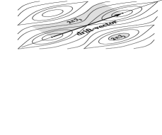
b) Level curves

c) Action variables

Figure 4.2. Characteristics of Morse function

If $g\in(g_{-},g_{+})$ then the set $\{\mathcal{Y}\in\mathbb{T}^{2}:\mathcal{H}=g\}$ consists of two connected components, each of them being again a trajectory on the torus, diffeomorphic to a circle, but now they are both non-contractible such that we obtain a non-trivial rotation number $d_{1}/d_{2}$. We in the case (b) of Proposition 4.1, and each trajectory is characterized by the points $g_{2}\in i_{2}$ and $g_{3}\in i_{3}$ on the two edges $i_{2}$ and $i_{3}$ of the Reeb graph; denote these trajectories on the torus $\mathbb{T}^{2}$ by $\widetilde{S}(g_{2,3},\mathcal{I}_{1})$. They induce a set of open trajectories $\widetilde{S}_{k}(g_{2,3},\mathcal{I}_{1})$, $k\in\mathbb{Z}$, on the covering space $\mathbb{R}^{2}_{y}$. The numbering of these trajectories we also discuss later. The drift vectors $d=d(i_{2})$ and $d=d(i_{3})$ corresponding to the edges $i_{2}$ and $i_{3}$ have opposite directions; we use the notation $d=d(\mathcal{I}_{1})$ for $i_{2}$ and $-d(\mathcal{I}_{1})$ for $i_{3}$.

Points on the Reeb graph corresponding to the extreme levels $g_{\text{min}}$ and $g_{\text{max}}$ are called end points; they correspond to the stable rest points of the Hamiltonian system (4.2). The points corresponding to the critical levels $g_{\pm}$ correspond to separatrices, including the saddle points $\mathcal{Y}_{\pm}$. Thus each interior point of any edge defines a closed trajectory or a closed oriented curve on the torus $\mathbb{T}^{2}$ where the orientation is given by the natural parameter $t$ (the time). We may parameterize the edges of the Reeb graph by the variable $g$ given by the value of $\mathcal{H}$; this defines one-to-one maps $g:[g_{\text{min}},g_{-})\to i_{1}$, $g:[g_{-},g_{+}]\to i_{2}$, $g:[g_{-},g_{+}]\to i_{3}$, and $g:(g_{+},g_{\text{max}}]\to i_{4}$.

4.3. Action variables and parameterization of the drift trajectories

One may also parameterize points on the edges of the Reeb graph by action variables

(4.3) $$\mathcal{I}_{2}=\frac{1}{2\pi}\int_{\sigma}^{\sigma+T}\mathcal{Y}_{1}(\tau)d\mathcal{Y}_{2}(\tau)-\frac{\mathcal{Y}_{2}(\sigma)(d(i_{j})\cdot a)_{1}}{2\pi}-\frac{(d(i_{j})\cdot a)_{1}(d(i_{j})\cdot a)_{2}}{4\pi}$$

with sign prescribed by the natural orientation, where $\sigma$ is an arbitrary real number.

As this definition of the action variable in the phase space $\mathbb{T}^{2}$ is somewhat different from the one in $\mathbb{R}^{2}$, let us explain formula (4.3).

The second and the third term are present only for the edges $i_{2}$ and $i_{3}$. The geometric interpretation of $|\mathcal{I}_{2}|$ for $i_{1,4}$ is standard: $2\pi|\mathcal{I}_{2}|$ is the square of the domain in $\mathbb{R}^{2}_{\mathcal{Y}}$ bounded by the corresponding closed trajectory (see Fig. 4.2b). Of course, here the action variables do not depend on parallel transport of the coordinate system on $\mathbb{R}^{2}_{\mathcal{Y}}$ and on the choice of the closed curve on $\mathbb{R}^{2}_{\mathcal{Y}}$. It is not difficult to show that $\mathcal{I}_{2}$ is positive for $i_{1}$ and negative for $i_{4}$, that $|\mathcal{I}_{2}|\leq a_{22}=a_{11}a_{22}/(2\pi)$, and that $\mathcal{I}_{2}=0$ in the end points $g_{\text{min,max}}$ of $i_{1,4}$.

The geometric interpretation of $\mathcal{I}_{2}$ for the edges $i_{2,3}$ is as follows. Denote by $L_{d}$ the straight line passing through the origin on the plane $\mathbb{R}^{2}_{\mathcal{Y}}$ in the direction of $d\cdot a$. Consider one of the lifts $\widetilde{S}_{0}=\bigl{(}\mathcal{Y}=\mathcal{Y}(\tau)\bigr{)}$ on $\mathbb{R}^{2}_{\mathcal{Y}}$ of the trajectory $\widetilde{S}$ on $\mathbb{T}^{2}_{\mathcal{Y}}$. Let us fix two points $\mathcal{Y}(\sigma)$ and $\mathcal{Y}(\sigma)+d(i_{2,3})\cdot a$ on this curve and project them onto $L_{d}$, such that we obtain some curved trapezium. The square of this trapezium is equal to $|2\pi\mathcal{I}_{2}|$, where $\mathcal{I}_{2}$ is defined by (4.3) (see Fig. 4.2b). This interpretation allows us to derive some simple properties of the action variable.

In contrast to the previous case we see that now $\mathcal{I}_{2}$ depends on the choice of a lift on the plane $\mathbb{R}_{\mathcal{Y}}^{2}$ of the trajectory (but it does not depend on this choice modulo $a_{11}a_{22}/2\pi)$, and it also depends on translations of the coordinates.

Let us fix next a certain continuous family of trajectories on the plane $\mathbb{R}^{2}_{\mathcal{Y}}$ corresponding to the edges $i_{j}$. Using the geometric interpretation of $\mathcal{I}_{2}$ it is easy to show that $\mathcal{I}_{2}$ increases along each edge $i_{j}$, such that we obtain a parameterization of all trajectories on the torus by means of the action variable $\mathcal{I}_{2}$, associated with the Reeb graph. If necessary, we write $\mathcal{I}_{2}^{j}$ to indicate that this action variable is associated with the edge $i_{j}$.

Obviously, $\mathcal{I}_{2}$ admits upper and lower limits along each edge. These limits depend also on $\mathcal{I}_{1}$ and given by

$$\mathcal{I}_{2}^{1+}(\mathcal{I}_{1})=\lim_{g\to g_{-}-0}\mathcal{I}_{2}^{1},\quad\mathcal{I}_{2}^{4-}(\mathcal{I}_{1})=\lim_{g\to g_{+}+0}\mathcal{I}_{2}^{4},\quad\mathcal{I}_{2}^{2\pm/3\pm}(\mathcal{I}_{1})=\lim_{g\to g_{\pm}\mp 0}\mathcal{I}_{2}^{2/3}.$$

One may calculate all the quantities $\mathcal{I}_{2}^{j\pm}$ as

$$\mathcal{I}_{2}^{j\pm}(\mathcal{I}_{1})=\int_{\gamma^{\pm}}\mathcal{Y}_{1}\,d\mathcal{Y}_{2},$$

where $\gamma^{\pm}$ is a separatrix connecting the corresponding saddle point $\mathcal{Y}_{\pm}(\mathcal{I}_{1})$ with the saddle point $\mathcal{Y}_{\pm}(\mathcal{I}_{1})+d$ on the plane $\mathbb{R}^{2}_{\mathcal{Y}}$. The numbers $\mathcal{I}_{2}^{1+}(\mathcal{I}_{1})$ and $\mathcal{I}_{2}^{4-}(\mathcal{I}_{1})$ are well defined, whereas the numbers $\mathcal{I}_{2}^{2\pm/3\pm}(\mathcal{I}_{1})$ are defined only up to $a_{11}a_{22}/2\pi$. If one fixes one of them, say, $\mathcal{I}_{2}^{2-}(\mathcal{I}_{1})$, then the others can be uniquely fixed by the “Kirchhof law”

$$\mathcal{I}_{2}^{1+}(\mathcal{I}_{1})=\mathcal{I}_{2}^{2-}(\mathcal{I}_{1})+\mathcal{I}_{2}^{3-}(\mathcal{I}_{1}),\qquad\mathcal{I}_{2}^{2+}(\mathcal{I}_{1})+\mathcal{I}_{2}^{3+}(\mathcal{I}_{1})=\mathcal{I}_{2}^{4-}(\mathcal{I}_{1})+\frac{1}{2\pi}a_{11}a_{22}.$$

We fix $\mathcal{I}_{2}(i_{3,4})$ in this way; the choice of $\mathcal{I}_{2}^{2-}(\mathcal{I}_{1})$ will be explained later. But for any choice of the action $\mathcal{I}_{2}$ the following inequalities and equalities are true:

(4.4) $$0<\mathcal{I}_{2}-\mathcal{I}_{2}^{2-/3-}(\mathcal{I}_{1})<\frac{1}{2\pi}a_{11}a_{22},$$

(4.5) $$\mathcal{I}_{2}^{1+}(\mathcal{I}_{1})+\Big{(}\mathcal{I}_{2}^{2+}(\mathcal{I}_{1})-\mathcal{I}_{2}^{2-}(\mathcal{I}_{1})\Big{)}+\Big{(}\mathcal{I}_{2}^{3+}(\mathcal{I}_{1})-\mathcal{I}_{2}^{3-}(\mathcal{I}_{1})\Big{)}+\mathcal{I}_{2}^{4-}(\mathcal{I}_{1})=\frac{1}{2\pi}a_{11}a_{22}.$$

Now we describe the numbering of the closed trajectories $S_{l}(g_{1,4},\mathcal{I}_{1})$. We define the multiindex $l$ as follows: Let us fix some extreme point $\mathcal{Y}_{\text{min,max}}$ of $\mathcal{H}$ in $\mathbb{R}^{2}_{\mathcal{Y}}$; we give the number $l=(0,0)$ to this point. It is clear that this choice determines the numbering of other extreme points by $\mathcal{Y}^{l}_{\text{max,min}}:=\mathcal{Y}_{\text{min,max}}+l\cdot a$, and the numbering of the corresponding trajectories $S_{l}(g_{1,4})$, depending continuously on $\mathcal{I}_{2}$ (they also depend on $\mathcal{I}_{1}$, see subsection 4.5). Indeed, if $S_{0}(g_{1,4})$ is defined by the equation $\mathcal{Y}=\mathcal{Y}(\tau,\mathcal{I})$, then the other trajectories are $S_{l}(g_{1,4},\mathcal{I}_{1}):=\mathcal{Y}=\mathcal{Y}(\tau,\mathcal{I})+l\cdot a$.

In contrast to the case (a), we enumerate the curves $\widetilde{S}_{k}$ by a single index $k\in\mathbb{Z}$. Fix a vector $f=(f_{1},f_{2})\in\mathbb{Z}^{2}$, conjugate to $d$, i. e. $d_{1}f_{1}+d_{2}f_{2}=1$, which always exists. Then we fix some open trajectory $\widetilde{S}_{0}$ corresponding to a certain point from the edge $i_{2}$ and give it the index $k=0$. According to the “Kirchhof law” for the action variables, we have to give this index also to the full family of open trajectories associated with both edges $i_{2}$, $i_{3}$ depending continuously on the corresponding action variable $\mathcal{I}_{2}$. If these trajectories are given by the equation $\widetilde{S}_{0}(g_{2,3},\mathcal{I}_{1}):\mathcal{Y}=\mathcal{Y}(\tau,\mathcal{I})$, then the open trajectories with index $k$ are $\widetilde{S}_{k}(g_{2,3},\mathcal{I}_{1}):\mathcal{Y}=\mathcal{Y}(\tau,\mathcal{I})-k\widehat{J}f\cdot a$.

Thus we see that the trajectories of the system on the torus and on the plane are parameterized by action variables $\mathcal{I}_{1}$ and $\mathcal{I}_{2}$, indices $l\in\mathbb{Z}^{2}$ or $k\in\mathbb{Z}$, and the edges of the Reeb graph; we include all these parameters to the notation in the next subsection. Finally, we have Figs. 4.2b and 4.2c for the trajectories on $\mathbb{R}^{2}_{\mathcal{Y}}$ (generally speaking, the curves $\mathcal{I}_{2}^{2}$ and $\mathcal{I}_{2}^{3}$ in Fig. 4.2c may coincide).

4.4. The Reeb graph in degenerate cases

Now consider now the case when $\mathcal{H}(\mathcal{I}_{1},\cdot)$ is not a simple Morse function.

There are two possible cases. Firstly, $\mathcal{H}(\mathcal{I}_{1},\cdot)$ can be a complex Morse function. Denote the corresponding value of $\mathcal{I}_{1}$ by $\mathcal{I}^{1}_{1}$, and if necessary add the subindex $\alpha$ for numbering of these critical values.

The regime of regular motion consists of contractible curves only, and the Reeb graph has the form described in Fig. 4.3a. This graph may be considered as a limit of the previous case as $g_{-}\to g_{+}$ such that and the edges $i_{2}$ and $i_{3}$ contract to a common point. The action variables are sketched in Fig. 4.3c, and the phase picture for the trajectories on the plane $\mathbb{R}^{2}$ is shown in Fig. 4.3b.

a) Reeb graph

b) Level curves

c) Action variables

Figure 4.3. Characteristics of Morse function: The degenerated case I.

Another limit case (Fig. 4.4) occurs if $g_{-}\to g_{\text{min}}$ and $g_{+}\to g_{\text{max}}$; all contractible trajectories disappear, and we are left with non-contractible trajectories only. In this case, $\mathcal{H}$ is not a Morse function, but we can still assign a Reeb graph to this situation (see Fig. 4.4a): we keep only the edges $i_{2}$ and $i_{3}$, and the action variables $\mathcal{I}^{1}_{2}$ and $\mathcal{I}^{4}_{2}$ show a similar behavior (Fig. 4.4c). We denote the corresponding values of the actions $\mathcal{I}_{1}$ by $\mathcal{I}^{2}_{1}$ and add, if necessary, the subindex $\alpha$ for numbering of these points.

a) Reeb graph

b) Level curves

c) Action variables

Figure 4.4. Characteristics of Morse function: Degenerated case II

4.5. The description of the averaged motion in 4-D phase space

Using the above considerations we now represent the global structure of the classical motion defined by $\mathcal{H}$ under assumption that the domain of the motion on the half-plane $(\mathcal{I}_{1}\geq 0,E)$ is separated into such (connected) subdomains, that the behavior of trajectories of the corresponding Hamiltonian systems for each of these subdomains is topologically equivalent and have the same rotation number (see Fig. 1.2). As before, we call these domains regimes. The interior points of each regime correspond to closed trajectories on tori $\mathbb{T}^{2}$; the boundary of the regimes is formed by the critical manifolds of the function $\mathcal{H}$ and by the left boundary $\mathcal{I}_{1}=0$.

A regime is called of boundary type and is denoted by $\mathcal{M}_{r}$ if it a certain part (of non-zero lenfth) of its boundary consists of extreme points of $\mathcal{H}$). On the plane $\mathbb{R}^{2}_{\mathcal{Y}}$ the corresponding level curves of the function $\mathcal{H}$ are families of closed trajectories, their preimages on the torus $\mathbb{T}^{2}$ are contractible trajectories with rotation number $0/0$, and they have no special direction. If we return back to the original four-dimensional phase space $\mathbb{R}^{4}_{p,x}$, for each interior point in these regimes we get a family of invariant Lagrangian manifolds of Hamiltonian $\mathcal{H}$. They are topological products of the cyclotron circles $S_{C}(\mathcal{I}_{1})$ and the closed curves $S_{l}(g_{1,4},\mathcal{I}_{1})$, and they are diffeomorphic to two-dimensional tori (we call them Liouville tori). We parameterize each point in $\mathcal{M}_{r}$ by the action variables $\mathcal{I}_{1}$ and $\mathcal{I}_{2}$, which belong to a certain domain on the plane $\mathbb{R}^{2}_{\mathcal{I}}$; to simplify the notation we denote these domains also by $\mathcal{M}_{r}$.

Thus each interior point $\mathcal{I}=(\mathcal{I}_{1},\mathcal{I}_{2})\in\mathcal{M}_{r}$ indicates a discrete family of invariant Lagrangian tori $\Lambda_{l}^{r}(\mathcal{I}_{1},\mathcal{I}_{2})$ in the original phase space $\mathbb{R}^{4}_{p,x}$ numbered by a multiindex $l=(l_{1},l_{2})\in\mathbb{Z}^{2}$ given by the numbering of the curves $S_{l}(g_{1,4},\mathcal{I}_{1})$.

If $\Lambda_{0}^{r}(\mathcal{I})$ is defined by the equations

(4.6) $$x_{1,2}=X_{1,2}(\mathcal{I},\varphi),\quad p_{1,2}=P_{1,2}(\mathcal{I},\varphi),$$

where $\varphi=(\varphi_{1},\varphi_{2})$ are angle variables conjugate to $\mathcal{I}=(\mathcal{I}_{1},\mathcal{I}_{2})\in\mathcal{M}_{r}$, then

$$\Lambda_{l}^{r}(\mathcal{I})=\big{\{}x=X(\mathcal{I},\varphi)+l\cdot a,\quad p_{1}=P_{1}(\mathcal{I},\varphi)+(l\cdot a)_{1},\quad p_{2}=P_{2}(\mathcal{I},\varphi)\big{\}}.$$

The action variables do not depend on $l$, and they are defined by (4.6) with $d=0$.

The remaining regimes are called interior regimes. We denote them by $\widetilde{\mathcal{M}}_{r}$ and use the symbol $\widetilde{\mathcal{M}}_{r}$ also for the domain of the corresponding action variables on the $(\mathcal{I}_{1},\mathcal{I}_{2})$-plane and $(\mathcal{I}_{1},E)$-plane. On the plane $\mathbb{R}^{2}_{\mathcal{Y}}$, the level sets of $\mathcal{H}$ are families of open curves with the main vector $d^{r}=(d_{1},d_{2})$, and their preimages on the torus $\mathbb{T}_{2}$ are non-contractible closed trajectories with rotation number $d_{1}/d_{2}$. In the original phase space $\mathbb{R}^{4}_{p,x}$, these trajectories are covered by a discrete set of the families of invariant two-dimensional Lagrangian manifolds $\widetilde{\Lambda}^{r}_{k}(\mathcal{I})$, $\mathcal{I}=(\mathcal{I}_{1},\mathcal{I}_{2})\in\widetilde{\mathcal{M}}_{r}$, of $\mathcal{H}$. They are products of the “cyclotron” circles $S_{C}(\mathcal{I}_{1})$ and the open curves $\widetilde{S}_{k}(g_{1,4},\mathcal{I}_{1})$ and are diffeomorphic to two-dimensional cylinders; for brevity we call $\widetilde{\Lambda}_{k}^{r}(\mathcal{I})$ Liouville cylinders.

The cylinders $\widetilde{\Lambda}_{k}^{r}(\mathcal{I})$ depend smoothly on $\mathcal{I}=(\mathcal{I}_{1},\mathcal{I}_{2})\in\widetilde{\mathcal{M}}_{r}$, their numbering by the index $k$ is induced by the numbering of the curves $\widetilde{S}_{k}(g_{1,4},\mathcal{I}_{1})$. Hence we have

$$\widetilde{\Lambda}^{r}_{k}(\mathcal{I})=\big{\{}x=X(I,\varphi)-k\widehat{J}f\cdot a,\quad p_{1}=P_{1}(\mathcal{I},\varphi)+k\widehat{J}f\cdot a,\quad p_{2}=P_{2}(\mathcal{I},\varphi,\varepsilon)\big{\}},$$

where the vector functions $P$ and $X$ define the Liouville cylinder $\widetilde{\Lambda}^{r}_{0}(\mathcal{I})$ by (4.6), $\varphi=(\varphi_{1},\varphi_{2})$ are the angle variables, and $\mathcal{I}\in\widetilde{\mathcal{M}}_{r}$.

We can give formulas for the action variables $\mathcal{I}_{1}$ and $\mathcal{I}_{2}$ directly on the tori and cylinders by:

$$\mathcal{I}_{1}=\frac{1}{2\pi}\int_{\varphi_{1}}^{\varphi_{1}+2\pi}p\,dx|_{\varphi_{2}=\text{const}},$$

(4.7) $$\mathcal{I}_{2}=\frac{1}{2\pi}\Big{(}\int_{\varphi_{2}}^{\varphi_{2}+2\pi}p\,dx|_{\varphi_{1}=\text{const}}+x_{1}(d^{r}\cdot a)_{2}+\frac{(d^{r}\cdot a)_{1}(d^{r}\cdot a)_{2}}{2}\Big{)},$$

where $(p,x)$ belongs to $\Lambda^{l}_{k}(\mathcal{I})$ or to $\widetilde{\Lambda}^{r}_{k}(I)$, respectively. Note that in the latter case $\mathcal{I}_{2}$ depends on index $k$, but in what follows we fix $\mathcal{I}_{2}$ by setting $k=0$ in the definition and using this action for parameterization of all $\widetilde{\Lambda}^{r}_{k}(\mathcal{I})$. We also assume that the families $\Lambda^{r}_{l}(\mathcal{I})$ and $\widetilde{\Lambda}^{r}_{k}(\mathcal{I})$ depend smoothly on $\mathcal{I}=(\mathcal{I}_{1},\mathcal{I}_{2})$ in the whole regime. Then, by fixing a certain cylinder from the interior regime associated with the edge $i_{2}$ of the Reeb graph and giving it the index $k=0$, we determine by the “Kirchhof law” the action the cylinders corresponding to the edge $i_{3}$.

It is well known that Lagrangian manifolds have the integer-valued homotopic invariants which are called Maslov indices and connected with the cycles on these manifolds. Obviously the Betty number (the rank of the cohomology group, or the number of basis cycles) of any Liouville torus $\Lambda^{r}_{l}$ is equal to two, hence $\Lambda^{r}_{l}$ have two Maslov indices and the Betty number of any Liouville cylinder $\widetilde{\Lambda}^{r}_{k}$ is equal to one, hence $\widetilde{\Lambda}^{r}_{k}$ has one Maslov index. Standard calculations lead to the following simple fact.

Proposition 4.2.

The Maslov index of the cycles $\gamma_{1,2}=(\varphi_{2,1}=\text{const})$ on any torus $\Lambda^{r}_{l}(\mathcal{I})$ is equal to $2\mod 4$. The Maslov index of the cycle $\gamma=(\varphi_{2}=\text{const})$ on any cylinder $\widetilde{\Lambda}^{r}_{k}(\mathcal{I})$ is also equal to $2\mod 4$.

Each non-degenerate point $\mathcal{I}=(\mathcal{I}_{1},0)$ of the extreme boundaries of the regimes $\mathcal{M}_{r}$ defines in $\mathbb{R}^{4}_{p,x}$ a degenerate torus, namely a closed trajectory, which is an isotropic manifold. In this case we have only cyclotron motion the drift is absent. The other non-degenerate boundaries between $\mathcal{M}_{r}$ and $\widetilde{\mathcal{M}}_{r}$ define separatrices of a one-dimensional Hamiltonian system with the Hamiltonian $\mathcal{H}$, which generates in $\mathbb{R}^{4}_{p,x}$ a two-dimensional invariant singular manifold of the Hamiltonian $\mathcal{H}$.

The critical points on the boundaries of the regimes induce degenerate singular invariant manifolds; these manifolds together with their neighborhoods are called atoms. Generally speaking, there exist infinitely many topological types of atoms, one can find some classifications some of them in [19, 20]. We restrict our consideration to the simplest situation described in the previous sections, then all critical values on the axis $\mathcal{I}_{1}$ are of the form $\mathcal{I}^{1/2}_{1,\alpha}$. The Morse function $\mathcal{H}$ changes its type, when $\mathcal{I}_{1}$ crosses these values (in our simplest case only rotation number changes; in more complicated problems a new Reeb graph can arise).

The left boundary $\mathcal{I}_{1}=0$ plays a special role in quantum applications, as it corresponds to the so-called low Landau bands. In the original phase space the corresponding trajectories belong the two-dimensional invariant subspace $\mathcal{I}_{1}=0$. This subspace presents only slow drift and the “cyclotron” motion is absent. All previous considerations concerning $\mathcal{H}$ remain valid, but now the “limit” Liouville tori $\Lambda_{l}^{r}(0,\mathcal{I}_{2})$ in $\mathbb{R}^{4}_{p,x}$ are just closed curves, and the “limit” Liouville cylinders $\widetilde{\Lambda}_{k}^{r}(0,\mathcal{I}_{2})$ are open curves with drift vector $d$; these curves are isotropic manifolds also.

The critical points $(\mathcal{I}_{1}=0$, $g=g_{\pm})$ can be considered as zero-dimensional singular manifolds. In the degenerate case $g_{+}(0)=g_{-}(0)$, there exist only two boundary regimes; this case is not generic, but it appears in connection with the Harper equation (see below). The other degenerate case is $g_{\text{min}}(0)=g_{-}(0)$ and $g_{\text{max}}(0)=g_{+}(0)$. It appears, for instance, when $v$ depends only on one variable. It seems that in this case one can separate the variables in the original spectral problem.

The angle points $\mathcal{I}=(0,0)$ in the left boundary correspond to the stable rest points of both the averaged and the original Hamiltonian $\mathcal{H}$ and $H$.

At last we remark that there is no reasonable definition of the Maslov index for an individual isotropic manifold $\Lambda\in\mathbb{R}^{2n}_{p,x}$, if $\dim\Lambda<n$, see e. g. [68, 13, 34, 9]. But if this manifold arises as the limit of a family of Lagrangian manifolds, one can associate with this manifold a Maslov index and make its use in the semiclassical approximation. Obviously, this applies to the problem under consideration.

4.6. Example

We illustrate the considerations of this section by the example (1.9) –(3.10). Let us consider first $\bar{H}$ instead of $\mathcal{H}$, then

$$g_{\text{min}}=-\Big{(}A\big{|}J_{0}(\sqrt{2\mathcal{I}_{1}})\big{|}+B\big{|}J_{0}(\beta\sqrt{2\mathcal{I}_{1}})\big{|}\Big{)},\quad g_{\text{max}}=A\big{|}J_{0}(\sqrt{2\mathcal{I}_{1}})\big{|}+B\big{|}J_{0}(\beta\sqrt{2\mathcal{I}_{1}})\big{|},$$

$$g_{\pm}=\pm\Big{|}A\big{|}J_{0}(\sqrt{2\mathcal{I}_{1}})\big{|}-B\big{|}J_{0}(\beta\sqrt{2\mathcal{I}_{1}})\big{|}\Big{|}.$$

The first series of critical points, $\mathcal{I}_{1,\alpha}^{1}$, $\alpha=1,2,\dots$, is obtained from the equations

$$J_{0}(\mathcal{I}_{1,\alpha}^{1})=0\quad\text{and}\quad J_{0}(\beta\mathcal{I}_{1,\alpha}^{1})=0.$$

The second series, $\mathcal{I}_{1,\alpha}^{2}$, $\alpha=1,2,\dots$, consists of the solutions of the equations

$$A\big{|}J_{0}(\mathcal{I}_{1,\alpha}^{2})\big{|}=B\big{|}J_{0}(\beta\mathcal{I}_{1,\alpha}^{2})\big{|}.$$

On the plane $(\mathcal{I}_{1},E)$, the boundary regimes are the sets (see Fig. 1.2)

$$\mathcal{I}_{1}+\varepsilon g_{\text{min}}(\mathcal{I}_{1})<E<\mathcal{I}_{1}+\varepsilon g_{-}(\mathcal{I}_{1}),\qquad\mathcal{I}_{1,\alpha}^{1}<\mathcal{I}_{1}<\mathcal{I}_{1,\alpha+1}^{1},$$

and

$$\mathcal{I}_{1}+\varepsilon g_{+}(\mathcal{I}_{1})<E<\mathcal{I}_{1}+\varepsilon g_{\text{max}}(\mathcal{I}_{1}),\qquad\mathcal{I}_{1,\alpha}^{1}<\mathcal{I}_{1}<\mathcal{I}_{1,\alpha+1}^{1};$$

the interior regimes are the sets

$$\mathcal{I}_{1}+\varepsilon g_{-}(\mathcal{I}_{1})<E<\mathcal{I}_{1}+\varepsilon g_{+}(\mathcal{I}_{1}),\qquad\mathcal{I}_{1,\alpha}^{2}<\mathcal{I}_{1}<\mathcal{I}_{1,\alpha+1}^{2}.$$

Note that the rotation number changes when $\mathcal{I}_{1}$ crosses these critical points.

The drift vectors of the interior regimes are

$$d=\begin{cases}(1,0)&\text{if $A\big{|}J_{0}(\sqrt{2\mathcal{I}_{1,\alpha}^{1}})\big{|}>B\big{|}J_{0}(\beta\sqrt{2\mathcal{I}_{1,\alpha}^{1}})\big{|}$},\\ (0,1)&\text{if $A\big{|}J_{0}(\sqrt{2\mathcal{I}_{1,\alpha}^{1}})\big{|}<B\big{|}J_{0}(\beta\sqrt{2\mathcal{I}_{1,\alpha}^{1}})\big{|}$.}\end{cases}$$

A simple calculation gives

$$\mathcal{I}^{1+}_{2}(\mathcal{I}_{1})=-\mathcal{I}^{4-}_{2}(\mathcal{I}_{1})=2\mathcal{I}^{2+}_{2}(\mathcal{I}_{1})=2\mathcal{I}^{3+}_{2}(\mathcal{I}_{1})=\frac{2}{\pi\beta}\int_{0}^{\Gamma(\mathcal{I}_{1})}\frac{1}{\xi}\log\left(\frac{1+\xi}{1-\xi}\right)d\xi,$$

(4.8) $$\mathcal{I}^{2+}_{2}(\mathcal{I}_{1})=\mathcal{I}^{3+}_{2}(\mathcal{I}_{1})=\frac{\pi}{\beta}-\frac{1}{2}\mathcal{I}^{1+}_{2}(\mathcal{I}_{1}),$$

where

$$\Gamma(\mathcal{I}_{1})=\left(\frac{A|J_{0}(\sqrt{2\mathcal{I}_{1}})|}{B|J_{0}(\beta\sqrt{2\mathcal{I}_{1}})|}\right)^{\pm 1},$$

and the sign in the exponential is such that $\Gamma\leq 1$.

Using $\mathcal{H}$ gives a discrepancy $O(\varepsilon^{2})$ in all above estimations.

5. Almost invariant manifolds of the original Hamiltonian

Definition 5.1.

Let $\Lambda=\{p=P(\varphi,\varepsilon),\quad x=X(\varphi,\varepsilon)\}\subset\mathbb{R}^{4}_{p,x}$ be either a two-dimensional Lagrangian manifold, diffeomorphic to a two-dimensional torus (or cylinder), or a smooth closed (or open) curve. Let $C>0$. We say that $\Lambda$ is an almost invariant manifolds of the Hamiltonian $H(p,x,\varepsilon)$ up to $O(e^{-C/\varepsilon})$ if

(5.1) $$H|_{\Lambda}=\text{const}+O(e^{-C/\varepsilon}),$$

and if a vector $\omega$ exists, such that

(5.2) $$\big{(}P(\varphi+\omega t,\varepsilon),X(\varphi+\omega t,\varepsilon)\big{)} O(e^{-C/\varepsilon}) t\in\mathbb{R}$$ satisfies the Hamiltonian system up to , uniformly in .

We call a family of two-dimensional almost invariant tori (respectively, cylinders) depending smoothly on action variables $\mathcal{I}\in\mathcal{M}$ almost Liouville tori (respectively, cylinders) of the Hamiltonian $H$.

According to this definition, the manifolds $\Lambda_{l}^{r}(\mathcal{I})$ and $\widetilde{\Lambda}_{k}^{r}(\mathcal{I})$ constructed in the previous section are almost Liouville tori or cylinders of the Hamiltonian $H$.

Of course, not all the applications need a construction of this accuracy. In some cases, it is reasonable to construct an averaged Hamiltonian $H^{K}$ up to $O(\varepsilon^{K+1})$ and to obtain “almost invariant” manifolds of $H$ with a discrepancy $O(\varepsilon^{K+1})$ (this means that in (5.1) and (5.2) one has $\varepsilon^{K+1}$ instead of $e^{-C/\varepsilon}$). In particular, $\bar{H}$ is the averaged Hamiltonian up to $O(\varepsilon^{2})$, and its invariant manifolds are almost invariant manifolds of $H$ but only up to $O(\varepsilon^{2})$.

Let us fix a sufficiently small $\delta$ and consider a boundary or an inner regime without $\delta$-neighborhood of the boundary formed by separatrices. If the regime includes the left boundary $\mathcal{I}_{1}=0$, then a neighborhood of this boundary (with a neighborhood of the singular points removed) also belongs to the non-singular part of this regime. Let us denote these non-singular parts of $\mathcal{M}_{r}$ or $\widetilde{\mathcal{M}}_{r}$ by $\mathcal{M}_{r,\delta}$ or $\widetilde{\mathcal{M}}_{r,\delta}$, respectively. The corresponding regimes for to $H^{K}$ we denote by $\mathcal{M}^{K}_{r,\delta}$ and $\widetilde{\mathcal{M}}^{K}_{r}$; they coincide with $\mathcal{M}_{r,\delta}$ and $\widetilde{\mathcal{M}}_{r,\delta}$ up to $O(\varepsilon^{K})$, and they have the same drift vectors. Moreover, the corresponding almost invariant tori and cylinders, $\Lambda^{r,K}_{l}$ and $\widetilde{\Lambda}^{r,K}_{l}$ have the same structure as $\Lambda^{r,K}_{l}$ and $\widetilde{\Lambda}^{r,K}_{l}$, and, in particular, their Maslov indices coincide.

6. Semiclassical spectral series

Now we are going to use the almost invariant manifolds described in the previous sections for constructing the spectral asymptotics for $\hat{H}$, like it was done in subsection 2.5. Let us emphasize again that in even in the simplest multidimensional problems there is usually no global asymptotic formula for the spectrum; it is useful to divide the spectrum into several parts, such that the asymptotic behavior of the spectrum is preserved in each of these parts. These parts together with the corresponding formulas for the spectrum are usually referred to as spectral series. According the fundamental correspondence principle of the quantum mechanics (connected with names of Bohr, Sommerfeld, Einstein, Ehrenfest, Brillouin, and others), the classification of spectral series is connected with the motions of the classical Hamiltonian system [27, 46, 60, 66, 67]. As a mathematical expression of this principle we use the method of the canonical operator developed by Maslov.

Now we are going to show how the correspondence pPrinciple appears in the problem under study.

Definition 6.1.

A pair $(\psi,E)$ with $\psi(x,h,\varepsilon)\in C^{\infty}({\mathbb{R}}^{2})$ and $E(h,\varepsilon)\in{\mathbb{R}}$ is called a quasimode of the operator $\hat{H}$ with error $O(h^{L}+\varepsilon^{K})$ if for any compact set $\Omega\subset{\mathbb{R}}^{2}$ there are positive numbers $A$ and $B$ satisfying $\|(\hat{H}-E)\Psi\|_{L_{2}(\Omega)}\leq Ah^{L}+B\varepsilon^{K}$.

From now on we fix some positive integer numbers $K$ and $L$; in the rest of the section we describe the construction of quasimodes for $\hat{H}$ with error $O(h^{L}+\varepsilon^{K})$.

6.1. Quasimodes associated with the almost Liouville tori

Consider a certain boundary regime $\mathcal{M}_{r,\delta}$ and the corresponding family of the almost Liouville tori $\Lambda_{l}^{r}(\mathcal{I},\varepsilon)$. As it was mentioned above, the asymptotics of the spectrum of $\hat{H}$ is defined by means of the canonical operator.

For each fixed $h>0$ let us choose a discrete subset of the values of the action variables $\mathcal{I}_{1}$ and $\mathcal{I}_{2}$, by the rules .

(6.1) $$\mathcal{I}_{1}=\mathcal{I}_{1}^{\mu}(h):=(\frac{1}{2}+\mu)h,$$

(6.2) $$\mathcal{I}_{2}=\mathcal{I}_{2}^{\nu}(h):=(\frac{1}{2}+\nu)h,$$

here $\mu$ and $\nu$ are integer numbers such that

(6.3) $$\big{(}\mathcal{I}_{1}^{\mu}(h),\mathcal{I}_{2}^{\nu}(h)\big{)}\in{\mathcal{M}}_{r,\delta}.$$

The conditions (6.1) and (6.2) are nothing but the necessary and sufficient condition for constructing the canonical operator on the tori $\Lambda^{r}_{l}\big{(}\mathcal{I}^{\mu}_{1}(h),\mathcal{I}_{2}^{\nu}(h),\varepsilon\big{)}$.

Proposition 6.1.

For any $(\mu,\nu)\in{\mathbb{Z}}_{+}\times{\mathbb{Z}}$ satisfying (6.3) there exist quasimodes $\big{(}\psi_{r,l}^{\mu,\nu}(x,h,\varepsilon),E^{\mu,\nu}_{r}(h,\varepsilon)\big{)}$ of the operator $\hat{H}$ with error $O(h^{L}+\varepsilon^{K})$; these quasimodes can be given by the equalities

$$\psi_{r,l}^{\mu,\nu}=\mathcal{K}_{\Lambda^{r}_{l}\big{(}\mathcal{I}^{\mu}_{1}(h),\mathcal{I}_{2}^{\nu}(h),\varepsilon\big{)}}\chi_{r,l}^{\mu,\nu},$$

$$\chi_{r,l}^{\mu,\nu}=1+O(h)\in C^{\infty}\Big{(}\Lambda^{r}_{l}\big{(}\mathcal{I}^{\mu}_{1}(h),\mathcal{I}^{\nu}_{2}(h),\varepsilon\big{)}\Big{)},$$

$$E^{\mu,\nu}_{r}=\mathcal{H}^{r}\big{(}\mathcal{I}^{\mu}_{1}(h),\mathcal{I}^{\nu}_{2}(h),\varepsilon\big{)}+O(h^{2}).$$

All the functions $\psi_{r,l}^{\mu,\nu}$ belong to $L^{2}({\mathbb{R}}^{2}_{x})$ and they can be expressed through each other as (cf. (2.36)):

(6.4) $$\psi_{r,l}^{\mu,\nu}(x,h,\varepsilon)=\psi_{r,0}^{\mu,\nu}(x-l\cdot a,h,\varepsilon)e^{-\frac{i}{h}l_{2}a_{22}x_{1}};$$

these functions are asymptotically localized near the projections $\pi_{x}\Lambda^{r}_{l}\big{(}\mathcal{I}^{\mu}_{1}(h),\mathcal{I}^{\nu}_{2}(h),\varepsilon\big{)}$ of the corresponding tori onto the $x$-plane as $h$ tends to $0$, i. e.

$$\lim_{h\to 0}\psi_{r,l}^{\mu,\nu}=0\text{ as }x\notin\pi_{x}\Lambda^{r}_{l}\big{(}\mathcal{I}^{\mu}_{1}(h),\mathcal{I}^{\nu}_{2}(h),\varepsilon\big{)}$$

One also has the estimate $\operatorname{dist}\big{(}E^{\mu,\nu}_{r}(h,\varepsilon),\operatorname{spec}\hat{H}\big{)}=O(h^{L}+\varepsilon^{K})$.

Remark.

The numbers $E^{\mu,\nu}_{r}$ as well as the functions $\psi_{r,l}^{\mu,\nu}$ depend also on $K$ and $L$; now we omit this dependence to simplify the notation, but sometimes we will write $E^{\mu,\nu}_{r,K,L}$ instead of $E^{\mu,\nu}_{r}$ to emphasize this dependence.

The proof directly follows from the general properties of the canonical operator; we describe the scheme of the proof in the Appendix.

Denote by $\Sigma^{r,\delta}_{K,L}(h,\varepsilon)$ the union of all possible points $E^{\mu,\nu}_{r}(h,\varepsilon)$. We call this set the semiclassical spectral series up to $O(h^{L}+\varepsilon^{K})$ corresponding to the boundary regime $\mathcal{M}_{r,\delta}$.

6.2. Quasimodes associated with the almost Liouville cylinders

Let us consider now a certain interior regime $\tilde{\mathcal{M}}_{r,\delta}$ and the corresponding family of the almost Liouville cylinders $\tilde{\Lambda}_{l}^{r}(\mathcal{I}_{1},\mathcal{I}_{2},\varepsilon)$.

To construct the canonical operator on these cylinders, we quantize only the action variable $\mathcal{I}_{1}$ by the rule (6.1), and $\mathcal{I}_{2}$ remains free. The integer numbers $\mu$ in (6.1) are such that

(6.5) $$\big{(}\mathcal{I}_{1}^{\mu}(h),\mathcal{I}_{2}\big{)}\in\mathcal{M}_{r,\delta}.$$

Proposition 6.2.

For any $(\mu,\mathcal{I}_{2})\in{\mathbb{Z}}_{+}\times{\mathbb{R}}$ satisfying (6.5) there exist quasimodes $\big{(}\tilde{\psi}_{r,k}^{\mu}(x,\mathcal{I}_{2},h,\varepsilon),\tilde{E}^{\mu}_{r}(\mathcal{I}_{2},h,\varepsilon)\big{)}$ of $\hat{H}$ with error $O(h^{L}+\varepsilon^{K})$; this quasimode is defined by

$$\tilde{\psi}_{r,k}^{\mu}=\mathcal{K}_{\tilde{\Lambda}^{r}_{k}\big{(}\mathcal{I}_{1}^{\mu}(h),\mathcal{I}_{2},\varepsilon\big{)}}\tilde{\chi}_{r,k}^{\mu},$$

$$\tilde{\chi}_{r,k}^{\mu}=1+O(h)\in C^{\infty}\Big{(}\tilde{\Lambda}^{r}_{k}\big{(}\mathcal{I}_{1}^{\mu}(h),\mathcal{I}_{2},\varepsilon)\big{)}\Big{)},$$

$$\tilde{E}^{\mu}_{r}(\mathcal{I}_{2},h,\varepsilon)=\mathcal{H}\big{(}\mathcal{I}_{1}^{\mu}(h),\mathcal{I}_{2},\varepsilon\big{)}+O(h^{2}).$$

The functions $\tilde{\psi}_{r,k}^{\mu}$ belong to $L^{2}_{\mathrm{loc}}(R^{2}_{x})$; they can be expressed through each other by the equality

(6.6) $$\tilde{\psi}_{r,k}^{\mu}(x,\mathcal{I}_{2},h,\varepsilon)=\tilde{\psi}_{r,0}^{\mu}(x+k(Jf)\cdot a,\mathcal{I}_{2},h,\varepsilon)e^{\frac{i}{h}f_{1}a_{22}x_{1}},$$

and enjoy the property

(6.7) $$\tilde{\psi}_{r,k}^{\mu}(x+{d}\cdot a,\mathcal{I}_{2},h,\varepsilon)=\tilde{\psi}_{r,k}^{\mu}(x,\mathcal{I}_{2},h,\varepsilon)e^{i(2\pi\mathcal{I}_{2}-({d}\cdot a)_{2}x_{1}-({d}\cdot a)_{1}({d}\cdot a)_{2}/2)},$$

where $d$ is the drift vector associated with the section $\tilde{\mathcal{M}}_{r,\delta}$, and the vector $f=(f_{1},f_{2})$ is dual to $d$, i.e. $d_{1}f_{1}+d_{2}f_{2}=1$. The functions $\tilde{\psi}_{r,k}^{\mu}$ are asymptotically localized near the projections $\pi_{x}\tilde{\Lambda}^{r}_{k}\big{(}\mathcal{I}^{\mu}_{1}(h),\mathcal{I}_{2},\varepsilon\big{)}$ of the corresponding cylinders onto the plane $x$ as $h$ tends to $0$.

For the numbers $\tilde{E}^{\mu}_{r}$ we have the estimate $\operatorname{dist}(\tilde{E}^{\mu}_{r}(\mathcal{I}_{2},h,\varepsilon),\operatorname{spec}\hat{H})=O(h^{L}+\varepsilon^{K})$.

In contrast to the boundary regimes, the points $\tilde{E}^{\mu}_{r}(\mathcal{I}_{2},h,\varepsilon)$ form vertical intervals in the domains $\tilde{\mathcal{M}}_{r,\delta}$ on the plane $(E,\mathcal{I}_{1})$. Denote by $\tilde{\Sigma}^{r,\delta}_{K,L}(h,\varepsilon)$ the union of all these intervals. We call this set the semiclassical up to $O(\varepsilon^{K}+h^{L})$ series corresponding to the interior regime $\tilde{\mathcal{M}_{r,\delta}}$.

6.3. Semiclassical spectrum

The union of the semiclassical series $\Sigma^{r,\delta}_{K,L}(h,\varepsilon)$ and $\tilde{\Sigma}^{r,\delta}_{K,L}(h,\varepsilon)$ corresponding to all regimes will be called the semiclassical up to $O(h^{L}+\varepsilon^{K})$ spectrum of the operator $\hat{H}$. We denote this set by $\Sigma_{K,L}(h,\varepsilon)$. An example of the structure of the semiclassical spectrum is shown in Fig. 1.3.

The statements of this section assert only that for arbitrary $K$ and $L$ one can find points from the spectrum of $\hat{H}$ in $O(h^{L}+\varepsilon^{K})$-neighborhood of the set $\Sigma_{K,L}(h,\varepsilon)$. Now a natural question arises: what kind of relationship between the exact and semiclassical spectrum of the operator $\hat{H}$ exist? In particular: does the whole spectrum of $\hat{H}$ belong to a certain $O(h^{L}+\varepsilon^{K})$-neighborhood of $\Sigma_{K,L}$? At the moment the answer is unknown, but we hope that it is positive. Our expectations are based, in particular, on the existence of such relationship between the semiclassical and the exact spectrum for the Sturm-Liouville problem (Section 2).

From the other side, each point of the semiclassical spectrum “asymptotically” has infinite degree of degeneracy in the sense that one can construct infinitely many linear independent quasimodes with the same semiclassical energy; if $\varepsilon$ is small enough, then there are no isolated points in $\Sigma_{K,L}$. As the exact spectrum does not have such properties (at least for rational values of the flux $\eta$), it is clear that the semiclassical and the exact spectrum do not coincide. Nevertheless, the semiclassical spectrum gives some information about the exact one. Before discussing this question, in Section $7$ we consider the situation when $\eta$ is a rational number and try to understand the meaning of the magneto-Bloch conditions (1.3) and (1.4) for the semiclassical analysis.

At last let us note that to construct semiclassical spectrum up to $O(h^{L}+\varepsilon^{K})$ it is enough to know only the averaged Hamiltonian $H^{K}$, see Section 5.

6.4. Relationship between $h$ and $\varepsilon$, and the widths of the Landau bands

Up to now, we did not assume yet any relationship between the parameters $h$ and $\varepsilon$, but in concrete physical problems such relationship may appear, say, $h=\varepsilon^{\kappa}$, $\kappa>0$. The energy levels $E^{\mu,\nu}_{r}(h,\varepsilon)$ and $\tilde{E}^{\mu}(\mathcal{I}_{2},h,\varepsilon)$ depend on the parameters $h$ and $\varepsilon$ in a regular way, and this means that increasing of $K$ and $L$ gives the correction to the energy levels corresponding to smaller numbers $K$ and $L$. We cannot say the same about the functions $\psi_{r,l}^{\mu,\nu}$ and $\tilde{\psi}_{r,k}^{\mu}$, because the ratio like $\varepsilon/h$ appears in the formulas for these functions. This fact does not allow to use the Raleigh-Schrödinger perturbation theory based on the small parameter $\varepsilon$ (as it was done e. g. in [63] for the case of fixed $h$).

The formulas for the semiclassical spectrum describe the well-known broadening of the Landau levels $E_{\mu}=\mathcal{I}_{1}^{\mu}(h)$ (these numbers are infinitely degenerated eigenvalues of $\hat{H}$ for $\varepsilon=0$) implied by the appearance of the electric field. For each $\mu$, the union of all the numbers $E^{\mu}_{r}(h,\varepsilon)$ and $E^{\mu,\nu}_{r}(\mathcal{I}_{2},\varepsilon,h)$ for all possible values of $\mu$, $\nu$, and $\mathcal{I}_{2}$ will be called the $\mu$th semiclassical Landau band and denoted by $L_{\mu}(h,\varepsilon)$.

If $\varepsilon(g_{\text{max}}(\mathcal{I}_{1}^{\mu})-g_{\text{min}}(\mathcal{I}_{1}^{\mu}))<h$, then the semiclassical Landau bands do not intersect, and one can calculate their widths:

(6.8) $$\operatorname{diam}L_{\mu}(h,\varepsilon)=\varepsilon(g_{\text{max}}(\mathcal{I}_{1}^{\mu})-g_{\text{min}}(\mathcal{I}_{1}^{\mu}))+O(\varepsilon^{2}+h^{2}).$$

For the example (1.7) we have

$$\operatorname{diam}L_{\mu}(h,\varepsilon)=2\varepsilon\big{(}A|J_{0}(\sqrt{2\mathcal{I}_{1}^{\mu}})|+B|J_{0}(\beta\sqrt{2\mathcal{I}_{1}^{\mu}})|+O(h^{2}+\varepsilon^{2})\big{)}.$$

For small and large values $\mathcal{I}^{\mu}_{1}$ one can use the estimates for the Bessel functions (see Section 3); in particular, for large $\mathcal{I}_{1}^{\mu}$ we have $\operatorname{diam}L_{\mu}(h,\varepsilon)\approx(\mathcal{I}_{1}^{\mu})^{-1/4}$. For the example (1.7) we have

$$\operatorname{diam}L_{\mu}(h,\varepsilon) \approx\varepsilon\big{(}A(2-\mathcal{I}_{1}^{\mu})+2B\beta(2-\mathcal{I}_{1}^{\mu})\big{)} \text{for small }\mathcal{I}_{1}^{\mu},$$

$$\operatorname{diam}L_{\mu}(h,\varepsilon) \approx\varepsilon\big{(}A\sqrt{\frac{2}{\pi\sqrt{2\mathcal{I}_{1}^{\mu}}}}(|\cos(\sqrt{2\mathcal{I}_{1}^{\mu}}-\pi/4)|+{}$$

$$~{}~{}{}+{\frac{B}{\sqrt{\beta}}}|\cos(\beta\sqrt{2\mathcal{I}_{1}^{\mu}}-\pi/4)|)\big{)} \text{for large }\mathcal{I}^{\mu}_{1}.$$

Note also that numerical considerations [51] show that the flux-energy diagram for the operator $\hat{H}$ for each Landau band in the plane $(E,\eta)$ looks like a butterfly (“Hofstadter butterfly”). Our assumptions about the smallness of $h$ and $\varepsilon$ mean that we consider the asymptotics of the spectrum corresponding to the upper part of the Hofstadter butterfly.

In this paper, we do not consider the structure of the spectrum in the neighborhood of the singular boundaries; the standard semiclassical approximation does not work there. It is clear that this asymptotics depends of the type of singularity, and in some cases is based of the parabolic cylinder functions. We will study this question in forthcoming papers.

6.5. Quantum averaging and the Harper-type equations

Basing on the Correspondence Principle, one can expect that there exist some quantum analogies of the averaging procedure (or, more generally, of the canonical transformation) in the classical mechanics. The study of such correspondence is developed now in several directions.

One can consider the Schrödinger equation as an infinite-dimensional Hamiltonian system and use for its solution different nontrivial generalizations of the classical averaging methods (see [11, 58, 85, 86]). This view on the Schrödinger equation with operator $\hat{H}$ was used in [11], and this study is connected with non-commutative analysis.

Another interpretation of the quantum averaging is based on the construction of an operator corresponding to the canonical change of variables, and this approach exploit the idea that a canonical transformation in the classical mechanics implies (with some accuracy) a unitary transformation in the quantum mechanics. This procedure approximately reduces the original spectral problem to the set of low-dimensional ones [54] and requires approximate solutions of some quantization problems. Such an approach for the problem under consideration gives the results formulated above. We have obtained these results by direct applying of the averaging and semiclassical methods; now let us try now to find a correspondence between the spectral problem for $\hat{H}$ and one-dimensional spectral problems basing on this interpretation of quantum averaging.

Roughly speaking, according to [54], to construct the first nontrivial approximation (with respect to parameters $h$ and $\varepsilon$) to the solutions of the equation $\hat{H}\Psi=E\Psi$ one has to solve approximately the equation

(6.9) $$\mathcal{H}\Big{(}\frac{1}{2}(-h^{2}\frac{\partial^{2}}{\partial\mathcal{Q}^{2}}+\mathcal{Q}^{2}),-ih\frac{\partial}{\partial\mathcal{Y}_{2}},\mathcal{Y}_{2},\varepsilon\Big{)}\Phi(\mathcal{Q},\mathcal{Y}_{2})=E\Phi(\mathcal{Q},\mathcal{Y}_{2}),$$

where all the operations are ordered according to the Weyl rule. The operator in the left-hand side commutes with the harmonic oscillator $\frac{1}{2}(-h^{2}{\partial^{2}}/{\partial\mathcal{Q}^{2}}+\mathcal{Q}^{2})$; this observation lets us write the solutions of (6.9) in the form $\Phi(\mathcal{Q},\mathcal{Y}_{2})=\psi_{\mu}(\mathcal{Q})w_{\mu}(\mathcal{Y}_{2})$, where $\psi_{\mu}$ is the $\mu$th eigenfunctions of the harmonic oscillator, and equation (6.9) is reduced to the family of equations

(6.10) $$\mathcal{H}\big{(}\mathcal{I}_{1}^{\mu}(h),-ih\frac{\partial}{\partial\mathcal{Y}_{2}},\mathcal{Y}_{2},\varepsilon\big{)}w_{\mu}(\mathcal{Q},\mathcal{Y}_{2})=Ew_{\mu}(\mathcal{Y}_{2}),\quad\mu\in{\mathbb{Z}}_{+}.$$

In particular, if we take $\bar{H}$ instead of $\mathcal{H}$ for the example (1.7), then the equations (6.10) will have the form

$$AJ_{0}(\sqrt{2\mathcal{I}_{1}^{\mu}})\dfrac{w_{\mu}(\mathcal{Y}_{2}+h)+w_{\mu}(\mathcal{Y}_{2}-h)}{2}\\ {}+BJ_{0}(\beta\sqrt{2\mathcal{I}_{1}^{\mu}})\cos\beta\mathcal{Y}_{2}\,w_{\mu}(\mathcal{Y}_{2})=\frac{E-\mathcal{I}_{1}^{\mu}}{\varepsilon}w_{\mu}(\mathcal{Y}_{2}),$$

i.e. they form a family of the Harper equations. Using this analogy, the equations (6.10) are usually called the Harper-type equations. Approximate solutions of each of them can be found using the usual one-dimensional WKB method. The description of the spectral asymptotics for equations of such kind using the Reeb graphs was obtained in [39]. Thefore, from this point of view, each semiclassical Landau band is described by a certain Harper-type equation; this equation depends on the band, and, therefore, different Landau bands can have different asymptotic structure. As follows from the preceding, the asymptotics of $\mu$th Landau band can be obtained by the quantization of the Reeb graph for the function $\mathcal{H}\big{(}\mathcal{I}_{1}^{\mu}(h),\mathcal{Y}_{1},\mathcal{Y}_{2},\varepsilon\big{)}$ considered as a function on the torus $\mathbb{R}^{2}/(a_{1},a_{2})$, what can be easily seen from Fig. 1.3.

7. The spectral asymptotics in the case of rational flux

Consider now the case when the flux $\eta:=a_{22}/h$ is a rational number, $\eta=N/M$, where $N$ and $M$ are mutually prime integer numbers and $M>0$. As mentioned in Section 1, in this case to each point from the spectrum of $\hat{H}$ one can assign a family of eigenfunctions satisfying the magneto-Bloch conditions (1.3) and (1.4). Crearly, the functions $\psi_{r,l}^{\mu,\nu}$ and $\tilde{\psi}_{r,k}^{\mu,r}$ do not satisfy these conditions, vbut, like in subsection 2.5, we can use them as a base for construction of quasimodes $\Psi^{r,j}_{\mu,\nu}$, $j=0,\ldots,M-1$, satisfying (1.3) and (1.4) (cf. [73, 87]). For convenience, we call the set of $M$ quasimodes satisfying the magneto-Bloch conditions as a family of magneto-Bloch quasimodes. We expect that this procedure will improve a detalization of the asymptotics to the spectrum.

7.1. Magneto-Bloch quasimodes corresponding to the boundary regimes

Let us consider a certain boundary regime $\mathcal{M}_{r,\delta}$ and the corresponding semiclassical spectral series $\Sigma^{r,\delta}_{K,L}(h,\varepsilon)$.

Proposition 7.1.

For any $(q_{1},q_{2})\in[0,1/M)\times[0,1)$ and any $(\mathcal{I}_{1}^{\mu},\mathcal{I}_{2}^{\nu})\in\mathcal{M}_{r,\delta}$ there exist exactly $M$ families of magneto-Bloch quasimodes of the form (cf. (2.18))

(7.1) $$\begin{gathered}\Psi^{r,s,j}_{\mu,\nu}(x,h,\varepsilon,q)=\sum_{l\in{\mathbb{Z}}^{2}}C^{s,j}_{l}(q_{1},q_{2},h)\psi_{r,0}^{\mu,\nu}(x-l\cdot a,h,\varepsilon)e^{-\frac{i}{h}x_{1}l_{2}a_{22}},\\ s,j=0,\ldots,M-1,\end{gathered}$$

such that all the functions $\Psi^{r,s,j}_{\mu,nu}$ are linearly independent. The coefficients $C^{s,j}_{l}(q)$ in (7.1) may be chosen in the following form (cf. (2.38)):

(7.2) $$C^{s,j}_{l_{1},l_{2}}(q_{1},q_{2},h)=\left\{\begin{array}[]{l}\exp\Big{[}-2\pi i(q_{1}l_{1}+q_{2}n)+2\pi i\eta l_{1}j-i\eta l_{2}a_{21}/2\Big{]},\\ \qquad\qquad\text{ if }l_{2}+j-s+nM=0,\quad n\in{\mathbb{Z}},\\ 0,\text{ otherwise.}\end{array}\right.$$

Here $l=(l_{1},l_{2})\in{\mathbb{Z}}^{2}$, the index $s=0,\ldots,M-1$ indicates the family of magneto-Bloch quasimodes, the index $j=0,\ldots,M-1$ indicates the number of a member in each of these families.

To prove this Proposition one has to substitute the sum (7.1) into (1.3) and (1.4), to equate the coefficients of $\psi_{0}^{\mu,\nu,r}(x-l\cdot a,h,\varepsilon)$, and to study the infinite linear system obtained.

We see that for each fixed value of the quasimomentum $q$ there are $M^{2}$ magneto-Bloch quasimodes corresponding to the same spectral value; in the other words, we have a degeneracy of degree $M^{2}$. We try to give an interpretation of this fact in Section 8.

Let us describe the structure of the functions $\Psi^{r,s,j}_{\mu,\nu}$. If the number $\mathcal{I}_{1}^{\mu}$ is small enough, then the asymptotic support of each of them consists of family of annulas. These annulas form strips separated by array of $M-1$ “empty” strips (see Fig. 7.1), where the corresponding quasimodes have order $O(h^{\infty})$. If $\eta$ tends to an irrational number, then $M\to\infty$, and only one strip is kept. This means, probably, that each of generalized eigenfunctions in the irrational flux case is asymptotically localized in such isolated strips. The diameters of the annulas depend on $\mathcal{I}_{1}^{\nu}$ (i.e., on the index of the Landau band); if the number $\mathcal{I}_{1}^{\mu}$ is large, then these annulas may intersect, and, probably, can cover the whole plane ${\mathbb{R}}^{2}_{x}$.

Figure 7.1. Asymptotic supports of magneto-Bloch quasimodes $\Psi^{r,s,j}_{\mu,\nu}$ on the $x$-plane

7.2. Magneto-Bloch quasimodes corresponding to the interior regimes

Now consider the quasimodes associated with the almost Liouville cylinders. Like in the previous subsection, the functions $\tilde{\psi}_{r,k}^{\mu}$ do not satisfy the magneto-Bloch conditions, and we again use them as a base for constructing magneto-Bloch quasimodes, i.e. we put

(7.3) $$\tilde{\Psi}^{j}_{\mu}(x,h,\varepsilon,q)=\sum_{k\in{\mathbb{Z}}}C^{j}_{k}(q_{1},q_{2},h)\ \tilde{\psi}_{k}^{\mu}(x,\mathcal{I}_{2},\varepsilon,h),\quad q=(q_{1},q_{2}).$$

To obtain the expression for the coefficients $C^{j}_{k}$, let us substitute the expressions (7.3) into (1.3) and (1.4), take into account the property (6.7), and then equate the coefficients of $\tilde{\psi}_{r,k}^{\mu}(x+k(Jf)\cdot a,\mathcal{I}_{2},\varepsilon,h)$ for all $k$. This system has the following form:

(7.4) $$\left\{\begin{array}[]{l}\displaystyle C^{j}_{k}\exp\Big{[}2\pi\frac{i}{h}\mathcal{I}_{2}+2\pi ik\eta-\frac{1}{2}i(2\pi d_{1}+a_{21}d_{2})d_{2}\Big{]}\\ \displaystyle\quad{}=C^{(j+d_{2})\operatorname{mod}M}_{k}\exp\Big{[}-2\pi id_{1}(q_{1}-j\eta)-i\eta d_{2}^{2}a_{21}/2+2\pi iL^{\prime}q_{2}\Big{]},\\ \displaystyle\qquad{}-L^{\prime}\leq\frac{d_{2}+j}{M}\leq(-L^{\prime}+1)-\frac{1}{M},\quad L^{\prime}\in\mathbb{Z},\\[3.0pt] \displaystyle C^{j}_{k-1}\exp\Big{[}i(k-1)f_{1}\eta(-2\pi f_{2}+a_{21}f_{1})\Big{]}\\ \displaystyle\quad{}=C^{(j+f_{1})\operatorname{mod}M}_{k}\exp\Big{[}2\pi if_{2}(q_{1}-j\eta)-i\eta f_{1}^{2}a_{21}/2+2\pi iL^{\prime\prime}q_{2}\Big{]},\\ \displaystyle\qquad{}-L^{\prime\prime}\leq\frac{f_{1}+j}{M}\leq(-L^{\prime\prime}+1)-\frac{1}{M},\quad L^{\prime\prime}\in\mathbb{Z}\end{array}\right.$$

(here and later by $A\operatorname{mod}M$ we mean the remainder after the integer division of $A$ by $M$). Obviously, the system depends crucially on the drift vector $d$ of the regime. Let us consider first the case $d=(\pm 1,0)$, then the system for the coefficients takes the form

(7.5) $$\begin{gathered}C^{j,\pm}_{k}e^{\pm 2\pi\frac{i}{h}(\mathcal{I}^{\pm}_{2}+ka_{22})}=C^{j,\pm}_{k}e^{-2\pi i(q_{1}-j\eta)},\quad k\in\mathbb{Z},\quad j=0,\ldots,M-1,\\ C^{(j+1)\operatorname{mod}M,\pm}_{k\pm 1}=C^{j,\pm}_{k}e^{i\eta a_{21}/2\pm ik\eta a_{21}}\sigma_{j},\\ k\in\mathbb{Z},\quad j=0,\ldots,M-1,\quad\sigma_{M-1}=e^{2\pi iq_{2}},\quad\sigma_{j}=1,\quad j\neq{M-1},\end{gathered}$$

where the index $\pm$ corresponds to $d=(\pm 1,0)$. We see that all the coefficients are uniquely determined by arbitrary chosen numbers $C^{j,\pm}_{0}$, $j=0,\ldots,M-1$, and we have, therefore, at most $M$ families of magneto-Bloch functions. For $s$th family, $s=0,\ldots,M-1$, set $C^{s,j,\pm}_{0}=\delta_{sj}$. It is easy to see that the equality

(7.6) $$\mathcal{I}_{2}^{\pm}=\mathcal{I}^{\pm}_{2}(n^{\pm},q_{1},h)=h\Big{(}\frac{n^{\pm}}{M}\mp q_{1}\Big{)},\quad n^{\pm}\in\mathbb{Z},$$

where $\mathcal{I}^{\pm}_{2}$ is the action variable corresponding to the drift vector $d=(\pm 1,0)$, is a necessary condition for the existence of solutions for (7.5). Obviously, the coefficients $C^{s,j,\pm}_{k}$ can be obtained from one set, say, $C^{0,j,\pm}_{k}$, by the shift of the index $j$ (and this means that really we have only one family of magneto-Bloch quasimodes). Therefore, the resulting coefficients can be chosen in the form

(7.7) $$C^{j,\pm}_{k}=\begin{cases}e^{i\eta k^{2}a_{21}/2+2\pi inq_{2}},&\text{ if }j\mp k+nM=0,\\ &\phantom{\text{ if }}n=n^{\pm}\tilde{N}+\tilde{n}M,\quad\tilde{n}\in\mathbb{Z},\\ 0,&\text{ otherwise},\end{cases}$$

where $\tilde{N}$ is an integer number such that for some $\tilde{M}\in\mathbb{Z}$ one has $\tilde{N}N+\tilde{M}M=1$.

(a)

(b)

Figure 7.2. The structure of the asymptotic support for the magneto-Bloch quasimodes $\Psi^{j}_{\mu}$: (a) the drift vector is $(1,0)$; (b) the drift vector is $(0,1)$

The expressions for the coefficients $C^{j}_{k}$ for the cases $d\neq(\pm 1,0)$ are rather complicated. At least, it is clear from the system (7.4) that all the coefficients are non-zero in this case. From this point of view, the case $d=(\pm 1,0)$ is the most useful one, because the asymptotic support of any magneto-Bloch quasimode is minimal in this case. From the other side, a situation with an arbitrary drift vector can be reduced to the case $d=(\pm 1,0)$, if one turns the coordinates, applies a gauge transformation, and transform the magneto-Bloch conditions accordingly. But it is important to emphasize, that this reduction is not global, because the drift vector can jump when passing from regime to regime even in the simplest cases, and to obtain reasonable formulas for the magneto-Bloch quasimodes one has to apply different transformation for different regimes (or, respectively, these transformations depend on the Landau band), and there exist no “globally good” coordinates.

8. Discussion and heuristic estimate of numbers of subbands

8.1. Relationship between the true and the semiclassical spectra. Dispersion relations

Let us give a qualitative description of the semiclassical spectrum in the rational flux case basing on the considerations of the previous section.

Let us consider a fixed semiclassical Landau band with index $\mu$. Its part corresponding to a boundary section is discrete, and each point $E^{\mu,\nu}_{r}$ is $M^{2}$-fold degenerated. The part of the band corresponding to an interior regime is continuous, but now each point $\tilde{E}^{\mu}_{r}(\mathcal{I}_{2},h,\varepsilon)$ is only $2M$-fold degenerated as $\tilde{E}^{\mu}_{r}(\mathcal{I}_{2},h,\varepsilon)$ can coincide for different edges of the Reeb graph. (Here we recall that we consider the situation with the simplest Reeb graphs, see §4.2; otherwise these estimations are estimations from below.) From the other side, if the number $\eta$ is rational, then the true spectrum of $\hat{H}$ has band structure and each point of the true spectrum is $M$-fold degenerated. Let us try to give an interpretation of the ambiguous degeneracy of the points $E^{\mu,\nu}_{r}$.

The existence of the isolated points $(\mathcal{I}_{1}^{\mu},\mathcal{I}_{2}^{\nu})$ can be explained then as follows. Our previous considerations have a non-avoidable error $O(h^{\infty}+\varepsilon^{\infty})$. Therefore, we can expect that these isolated points really approximate subbands of width $O(h^{\infty}+\varepsilon^{\infty})$. The presence of $M^{2}$-fold degeneracy of these points probably means that in a neighborhood of each such point there are $M$ true spectral subbands (minibands) of the operator $\hat{H}$. (Additional arguments can be given basing on the following idea: the formulas (7.2) realize a representation of the magnetic translation group on the space of asymptotic eigenfunctions; as all such representations are $M$-dimensional [95], small variation of parameters leads to the splitting of each energy level into $M$ numbers.) Enumerate these bands by an index $s=0,\ldots,M-1$, then the dispersion relations $E^{\mu,\nu}_{r,s}(q_{1},q_{2},h,\varepsilon)$ in all these minibands look as follows:

$$E^{\mu,\nu}_{r,s}(q_{1},q_{2},h,\varepsilon)=E^{\mu,\nu}_{r,K,L}(h,\varepsilon)+O(h^{L}+\varepsilon^{K})$$

for any positive $K$ and $L$. Therefore, the approximation used does not give expressions for the dispersion relations, and the presence of the separation of bands cannot be found rigorously. Nevertheless, this splitting is supported by the analogy with the one-dimensional periodic problem (subsection 2.3). Assume that there exists a function $\breve{\psi}^{\mu,\nu}_{r,0}$ such that the true magneto-Bloch functions can be represented as

$$\Psi^{r,s,j}_{\mu,\nu}(x,q,h,\varepsilon)=\sum_{l=(l_{1},l_{2})\in\mathbb{Z}^{2}}C^{s,j}_{l}(q,h)\breve{\psi}^{\mu,\nu}_{r,0}(x-l\cdot a,h,\varepsilon)e^{-\frac{i}{h}l_{2}a_{22}x_{1}},$$

where the coefficients $C^{s,j}_{l}$ are defined in Proposition 7.1. Similarly to (2.23) we obtain that if $\Psi_{1}$ and $\Psi_{2}$ are (generalized) eigenfunctions of $\hat{H}$ with eigenvalues $E_{1}$ and $E_{2}$, then

(8.1) $$E_{1}-E_{2}=\dfrac{\Re\oint\limits_{\partial D}\Big{[}h^{2}(\overline{\Psi}_{1}\nabla\Psi_{2}-\nabla\overline{\Psi}_{1}\Psi_{2})-ih\overline{\Psi}_{1}\Psi_{2}A\Big{]}ds}{\Re\int_{D}\overline{\Psi}_{1}\Psi_{2}dx_{1}dx_{2}},$$

where $A=(-x_{2},0)$ is the vector potential of the magnetic field, $ds=(dx_{1},dx_{2})$, and $D\subset\mathbb{R}^{2}$ is any domain with boundary $\partial D$. Assume that the asymptotic support of $\breve{\psi}^{\mu,\nu}_{r,0}$ belongs to the unit cell generated by the vectors $a_{1}$ and $a_{2}$. Let us choose this unit cell as the domain $D$. Put $\Psi_{1/2}=\Psi_{\mu,\nu}^{r,s,j}(x,q^{1/2},h,\varepsilon)$ and $E_{1/2}=E^{\mu,\nu}_{r,s}(q^{1/2},h,\varepsilon)$. Substituting all these expressions into (8.1), one obtains (cf. (2.25)):

(8.2) $$E^{\mu,\nu}_{r,s}(q^{1},h,\varepsilon)-E^{\mu,\nu}_{r,s}(q^{2},h,\varepsilon)\\ {}\approx\sum_{l_{1},n=\overline{0,\pm 1}}\rho^{\mu,\nu,r}_{n,l_{1}}(e^{2\pi(q^{1}_{1}l_{1}+q^{1}_{2}n)}-e^{2\pi(q^{2}_{1}l_{1}+q^{2}_{2}n)})e^{2\pi i\eta l_{1}s},$$

where

$$\rho^{\mu,\nu,r}_{n,l_{1}}=\dfrac{\Re\oint_{\partial D}\Big{[}h^{2}({{\breve{\psi}}^{\mu,\nu}_{r,l}}\overline{\nabla{\breve{\psi}}^{\mu,\nu}_{r,0}}-\nabla{\breve{\psi}}^{\mu,\nu}_{r,l}\overline{{\breve{\psi}}^{\mu,\nu}_{r,0}})-ih\overline{{\breve{\psi}}^{\mu,\nu}_{r,0}}{\breve{\psi}}^{\mu,\nu}_{r,l}A\Big{]}ds}{\Re\int_{D}\big{|}\breve{\psi}^{\mu,\nu}_{r,0}\big{|}^{2}dx_{1}dx_{2}}=O(h^{\infty}),$$

$$l=(l_{1},nM).$$

In the interior regimes, we have the following dependences of the energy on the quasimomenta (semiclassical dispersion relations):

$$E^{\pm}(q,h)=E_{n^{\pm}}(q,h,\varepsilon)=E^{\mu}_{r}\big{(}\mathcal{I}_{2}^{\pm}(q,n^{\pm},h),h,\varepsilon\big{)}.$$

Consider the case with drift vector $(\pm 1,0)$, then these functions depends essentially only on $q_{1}$, and the dependence on $q_{2}$ is absent up to $O(h^{L}+\varepsilon^{K})$. As some of these functions increases in $q_{1}$ and others decreases, for some critical values of $q_{1}=q_{1}^{*}$ one has

$$E_{n_{1}^{+}}(q_{1}^{*},h,\varepsilon)=E_{n_{2}^{-}}(q_{1}^{*},h,\varepsilon)$$

(see Fig. 8.2). For the example (1.7), these points correspond to the values $\mathcal{I}^{2/3}_{2}=h(2n+1)/(2M)$. We can expect that these points together with the “end” points $\mathcal{I}^{2/3}=hn/M$ are $O(h^{\infty}+\varepsilon^{\infty})$-approximations of the gaps in the spectrum of $\hat{H}$, see Fig. 8.2. This expectation is based, in particular, on the analogy with the one-dimensional periodic problem (subsection 2.5), cf. [39]. If the interior regime has the drift vector other than $(\pm 1,0)$, then these semiclassical dispersion relations depend on a certain linear combination of $q_{1}$ and $q_{2}$.

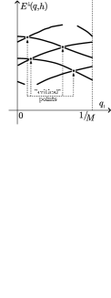
Figure 8.1. Semiclassical dispersion relations

Figure 8.2. True dispersion relations (hypotesis)

Our hypotesis about the structure of the Landau bands are illustrated in Fig. 1.5.

Note that in our spectral estimates we have used the almost invariant Liouville tori and cylinders. It is known that even an exponentially small correction, which is kept after applying the averaging procedure, can destroy some of these objects, and non-Kolmogorov sets may appear. These fact implies the following question: what do non-Kolmogorov sets mean for the exact spectrum of the operator $\tilde{H}$, in particular in situation when the flux $\eta$ is rational? It seems that the answer cannot be given using the additive asymptotics.

8.2. Heuristic estimate for the numbers of subbands

If the hypotesys of the previous subsection is true, then it is possible to count the number of spectral subbands corresponding to a fixed (semiclassical) Landau band. Let us consider a certain fixed value $\mathcal{I}^{\mu}_{1}$.

For the edge $i_{1}$ of the corresponding Reeb graph, the number of the quantization points $\mathcal{I}_{2}^{\nu}$ is equal approximately to $-\mathcal{I}_{2}^{1+}/h$, and for the edge $i_{4}$ this number is equal to $\mathcal{I}_{2}^{4-}/h$. Each of these points subbands, so the end edges $i_{1}$ and $i_{4}$ give us approximately (modulo singular boundaries effects)

$$\frac{M}{h}\ (\mathcal{I}_{2}^{1+}-\mathcal{I}_{2}^{4-})=2\pi N\ \frac{\mathcal{I}_{2}^{1+}-\mathcal{I}_{2}^{4-}}{a_{11}a_{22}}$$

bands.

The expected numbers of subbands implied by the edges $i_{2/3}$ depends may depend on the symmetry properties of the potential $v$. For the example (1.7), we obtain approximately (again modulo singular boundaries effects):

$$2M\ \frac{\mathcal{I}_{2}^{2+}-\mathcal{I}_{2}^{2-}}{h}=4\pi N\ \frac{\mathcal{I}_{2}^{2+}-\mathcal{I}_{2}^{2-}}{a_{11}a_{22}}$$

bands.

Therefore, the total number of the subbands is approximately equal to

$$2\pi N\ \frac{\mathcal{I}_{2}^{1+}-\mathcal{I}_{2}^{4-}+\mathcal{I}_{2}^{2+}-\mathcal{I}_{2}^{2-}+\mathcal{I}_{2}^{3+}-\mathcal{I}_{2}^{3-}}{a_{11}a_{22}}$$

(we have used the symmetry property $\mathcal{I}^{2+}_{2}-\mathcal{I}^{2-}_{2}=\mathcal{I}^{3+}_{2}-\mathcal{I}^{3-}_{2}$) and the latter number is precisely equal to $N$ according to the Kirchhoff law (4.5) for the action variables.

8.3. Correspondence to difference equations

In conclusion, let us discuss the relationship between the problem under consideration and the difference equation (subsection 6.5) in the rational flux case. It is known that the spectrum of a rational Harper-like operator with flux $\eta=N/M$ consists of $N$ bands [39]; the presence of $M$-grouped bands corresponding to finite motion (boundary regimes) was studied numerically for some cases [39]. Therefore, we can expect, that our hypotesis about the spectrum of $\hat{H}$, in particular, the estimate of the number of subbands in each Landau band is not connected with the simplicity of the potential.

Appendix A The canonical operator and spectral estimates

As it was noted above, the asymptotics of the spectrum can be found using the canonical operator. Let us remind some basic properties of the canonical operator; a more detailed constructions can be found, for example, in [60] or [68].

Let $\Lambda$ be a closed Lagrangian manifolds without boundary in the space $\mathbb{R}^{2n}_{p,x}$. The canonical operator $\mathcal{K}_{\Lambda}$ corresponding to this manifold maps from $C^{\infty}(\Lambda)$ to $C^{\infty}(\mathbb{R}^{n})$, and for any function $f\in C^{\infty}(\Lambda)$ one has $Kf=0$ outside certain $\delta$-vicinity of the projection $\pi_{x}\Lambda$ The canonical operator on $\Lambda$ can be constructed iff

$$\frac{1}{2\pi}\oint_{\gamma}p\,dx=h\Big{(}n+\frac{{\rm Ind}~{}\gamma}{4}\Big{)},\quad n\in\mathbb{Z},$$

for each basis cycle on $\Lambda$, where ${\rm Ind}$ denotes the Maslov index. Applying this consideration to the tori $\Lambda^{r}_{l}$ and the cylinders $\tilde{\Lambda}^{r}_{k}$ we obtain the quantization condition (6.1) and (6.2) for the tori (they have two basis cycles), and (6.1) for the cylinders (only one basis cycle).

The following commutation formula is one of the most important properties of the canonical operator.

Proposition A.1 (Commutation formula).

Assume that $\Lambda$ is an invariant Lagrangian manifold of a Hamiltonian system for a certain Hamiltonian $H$, and that on $\Lambda$ there exists a volume form which is also invariant under the Hamiltonian system. There exists a sequence of differential operators $\{R^{j}\}_{j=1}^{\infty}$,

$$R^{j}:C^{\infty}(\Lambda)\mapsto C^{\infty}(\Lambda),$$

with smooth coefficients such that for any function $\varphi\in C^{\infty}(\Lambda)$ and any number $N\in\mathbb{N}$ one has

(A.1) $$\hat{H}\mathcal{K}_{\Lambda}\varphi=\mathcal{K}_{\Lambda}\Big{(}\sum_{j=0}^{N}(ih)^{j}R^{j}\varphi\Big{)}+O(h^{N+1}).$$

In particular, $R^{0}$ is the operator of multiplication by the scalar function $H|_{\Lambda}$, and

$$R^{1}=-\frac{d}{dt}\Leftrightarrow-\frac{\partial H}{\partial p}\frac{\partial}{\partial x}+\frac{\partial H}{\partial x}\frac{\partial}{\partial p}.$$

Here $\hat{H}$ is the Weyl quantization of the Hamiltonian $H$.

Now let us try to construct an approximate solutions of the equation $\hat{H}\Psi=E\Psi$ up to $O(h^{L}+\varepsilon^{K})$ basing on the commutation formula and almost Liouville tori $\Lambda^{r}_{l}$. Assume that the conditions (6.1) and (6.2) are satisfied. Let us find requested solutions in the form

$$\Psi=\mathcal{K}_{\Lambda^{r}_{l}}u,\quad u=\sum_{j=0}^{L-1}(ih)^{j}u_{j},\quad u_{j}\in C^{\infty}(\Lambda^{r}_{l}),\quad E=\sum_{j=0}^{L-1}(ih)^{j}\lambda_{j}.$$

Applying the commutation formula, we obtain

$$(\hat{H}-E)\Psi=\Big{\{}\sum_{n=0}^{L-1}\sum_{s+j=n}(R^{j}-\lambda_{j})u_{s}\Big{\}}+O(h^{L}+e^{-C/\varepsilon})$$

(the presence of the term $O(e^{-C/\varepsilon})$ is implied by the fact that the manifolds $\Lambda^{r}_{l}$ are not invariant under $H$, but only almost invariant). We request that the expression in the curly brackets vanishes at least up to $O(\varepsilon^{K})$ for some $K>0$.

For $n=0$ we obtain the equation $(H|_{\Lambda^{r}_{l}}-\lambda_{0})u_{0}=0$, and we can put $\lambda_{0}=\mathcal{H}|_{\Lambda^{r}_{l}}$ and $u_{0}=1$.

For $n=1$ we obtain $(d/dt+\lambda_{1})u_{0}=0$ and we set $\lambda_{1}=0$.

The equations for $n\geq 2$ have the form

$$-\frac{d}{dt}u_{n-1}=\sum_{j=0}^{n-2}(R^{n-j}-\lambda_{n-j})u_{j}$$

(they are called homological equations). Let us show that all these equations can be solved up to $O(\varepsilon^{m})$, where $m$ is arbitrary positive number. To do this, let us note first, that the operator $d/dt$ on each torus can be written as

$$\frac{d}{dt}=\omega_{1}\frac{\partial}{\partial\varphi_{1}}+\omega_{2}\frac{\partial}{\partial\varphi_{2}},\quad\omega_{1/2}=\frac{\partial\mathcal{H}}{\partial\mathcal{I}_{1/2}}\Big{|}_{\Lambda^{r}_{l}}.$$

It is important for us that $\omega_{1}=1+O(\varepsilon)$ and $\omega_{2}=O(\varepsilon)$; both these numbers do not depend on $\varphi_{1}$ and $\varphi_{2}$.

Rewrite all the homological equations in a common form

(A.2) $$\frac{d}{dt}f=E+g,\quad g\in C^{\infty}(\Lambda^{r}_{l}).$$

Let us expand all the functions into their Fourier series:

$$f=\sum_{(k_{1},k_{2})\in\mathbb{Z}^{2}}f_{k_{1},k_{2}}e^{i(k_{1}\varphi_{1}+k_{2}\varphi_{2})},\quad g=\sum_{(k_{1},k_{2})\in\mathbb{Z}^{2}}g_{k_{1},k_{2}}e^{i(k_{1}\varphi_{1}+k_{2}\varphi_{2})}.$$

Substituting these series into (A.2), we obtain formally:

$$f_{k_{1},k_{2}}=\frac{1}{k_{1}\omega_{1}+k_{2}\omega_{2}}g_{k_{1},k_{2}},\quad E=-g_{0,0}.$$

Note that these coefficients $f_{k_{1},k_{2}}$ can be very large because of the denominator, and the function $f$ is, generally speaking, not defined. To avoid this obstacle, let us use additional estimates. As $g\in C^{\infty}$, its Fourier coefficients decay very fast, and for any $\alpha>0$ there exists positive numbers $C(\alpha)$ and $N(\alpha)$ such that $|g_{k_{1},k_{2}}|\leq C(\alpha)/(|k_{1}|+|k_{2}|)^{\alpha}$ as $|k_{1}|+|k_{2}|>N(\alpha)$. Let us put $\alpha=2m$.

Introduce a set $Q(\varepsilon,\alpha)$ as follows:

$$Q(\varepsilon,\alpha)=\Big{\{}(k_{1},k_{2})\in\mathbb{Z}^{2}:~{}|k_{1}|+|k_{2}|\leq N(\alpha)\Big{\}}\\ {}\cup\Big{\{}(k_{1},k_{2})\in\mathbb{Z}^{2}:~{}|k_{2}|\leq\frac{1}{\sqrt{\varepsilon}}\Big{\}}.$$

Clearly, $|k_{1}\omega_{1}+k_{2}\omega_{2}|\geq 1/2$ as $(k_{1},k_{2})\in Q(\varepsilon,\alpha)$ and $\varepsilon$ is small enough.

Now set

$$G=\sum_{(k_{1},k_{2})\in Q(\varepsilon,\alpha)}g_{k_{1},k_{2}}e^{i(k_{1}\varphi_{2}+k_{2}\varphi_{2})},\quad\tilde{g}=g-G.$$

The equation $df/dt=G$ can be solved in Fourier series, and the function $\tilde{g}$ gives a discrepancy $O(\varepsilon^{K})$, because

$$\tilde{g}_{k_{1},k_{2}}\leq C(\alpha)/(|k_{1}|+|k_{2}|)^{\alpha}\leq C(\alpha)\varepsilon^{K}.$$

Therefore, we can construct a function $u\in L^{2}(\mathbb{R}^{2})$ and a number $E\in\mathbb{R}$ such that $\|u\|_{L^{2}}\geq c>0$ and $\|(\hat{h}-E)u\|_{L^{2}}=O(h^{L}+\varepsilon^{K})$ as $h,\varepsilon\to 0$. Then

(A.3) $$\operatorname{dist}(E,\operatorname{spec}\hat{H})\leq\frac{\|(\hat{H}-E)u\|}{\|u\|}=O(h^{L}+\varepsilon^{K}).$$

The same procedure can be applied to each of the quantized cylinders $\tilde{\Lambda}^{r}_{k}$, but as a result we obtain a function $u\in L^{2}_{\text{loc}}$ and a number $E\in\mathbb{R}$ such that

(A.6) $$\begin{gathered}u(x+d\cdot a,h,\varepsilon)=u(x,h,\varepsilon)e^{\frac{i}{h}\big{(}2\pi\mathcal{I}_{2}-(d\cdot a)_{1}x_{1}-\frac{1}{2}(d\cdot a)_{1}(d\cdot a)_{2}\big{)}},\\ \|u\|_{L^{2}(\Pi)}\geq c>0,\text{ and }\|(\hat{H}-E)u\|_{L^{2}(\Pi)}=O(h^{L}+\varepsilon^{K}),\end{gathered}$$

where

$$\Pi=\big{\{}x=\tau_{1}(d\cdot a)+\tau_{2}J(d\cdot a),\quad\tau_{1}\in[0,1],\quad\tau_{2}\in\mathbb{R}\big{\}}.$$

As such function $u$ does not belong to $L^{2}_{\mathrm{loc}}(\mathbb{R}^{2})$, one cannot apply the inequality (A.3) directly.

Proposition A.2.

Let a function $u$ and a number $E$ satisfy the conditions (A.6), then $\operatorname{dist}(E,\operatorname{spec}\hat{H})=O(h^{L}+\varepsilon^{K})$.

Proof.

Introduce new coordinates

$$y=Ax,\quad A=\begin{pmatrix}\alpha&\beta\\ -\beta&\alpha\end{pmatrix},\quad\begin{pmatrix}\alpha\\ \beta\end{pmatrix}=\frac{d\cdot a}{|d\cdot a|}$$

and a function

$$S(y)=\frac{1}{2}(-\alpha\beta y_{1}^{2}+\alpha\beta y_{2}^{2}+2\beta^{2}y_{1}y_{2}).$$

Define a unitary operator $\hat{U}$ in $L^{2}(\mathbb{R}^{2})$ by the rule

$$f(x)\stackrel{{\scriptstyle\hat{U}}}{{\mapsto}}g(y)=e^{-\frac{i}{h}S(y)}f(A^{-1}y);$$

it is easy to see that $U$ is well-defined also on $L^{2}_{\mathrm{loc}}(\mathbb{R}^{2})$. Now we set $\tilde{H}=\hat{U}\hat{H}\hat{U}{}^{-1}$, i. e.

$$\tilde{H}=\frac{1}{2}\Big{(}-ih\frac{\partial}{\partial y_{1}}+y_{2}\Big{)}^{2}+\frac{1}{2}\Big{(}-ih\frac{\partial}{\partial y_{2}}\Big{)}^{2}+\varepsilon w(y),\quad w(y)=v(A^{-1}y).$$

As the operator $\hat{U}$ is unitary, the spectra of $\hat{H}$ and $\tilde{H}$ coincide.

Put $\varphi=\hat{U}u$, then

$$\varphi(y_{1}+|d\cdot a|,y_{2},h,\varepsilon)=\varphi(y_{1},y_{2},h,\varepsilon)e^{2\pi\frac{i}{h}\mathcal{I}_{2}}.$$

Denote

$$\tilde{\Pi}_{s}=\Big{\{}(y_{1},y_{2})\in\mathbb{R}^{2}:\quad-s|d\cdot a|\leq y_{1}\leq s|d\cdot a|\Big{\}},\quad s\in\mathbb{Z},$$

Note that

$$\|f\|_{L^{2}(\tilde{\Pi}_{s})}=\sqrt{s}\|f\|_{L^{2}(\tilde{\Pi}_{1})}$$

for any function satisfying $f(y_{1}+|d\cdot a|)=e^{i\alpha}f(y_{1},y_{2})$, $\alpha\in\mathbb{R}$; in particular, this holds for $f=\varphi$ and for $f=\Phi:=(\tilde{H}-E)\varphi$.

Choose now a smooth function $e(\xi)$ such that

$$0\leq e(\xi)\leq 1,$$

$$e(\xi)=1 \quad\text{ as }\xi\in(-|d\cdot a|,|d\cdot a|),$$

$$e(\xi)=0 \quad\text{ as }\xi\notin(-2|d\cdot a|,2|d\cdot a|),$$

and choose a constant $C_{0}$ such that

$$|e|+|e^{\prime}|+|e^{\prime\prime}|\leq C_{0}.$$

Put $e_{s}(y_{1},y_{2}):=e(y_{1}/s)$. Now we have the following chain of equalities and inequalities:

$$\sqrt{s}\operatorname{dist}\big{(}E,\operatorname{spec}\hat{H}\big{)}\|\varphi\|\leq\operatorname{dist}\big{(}E,\operatorname{spec}\hat{H}\big{)}\|e_{s}\varphi\|_{L^{2}(\tilde{\Pi}_{s})}$$

$$\leq\Big{\|}\big{(}\tilde{H}-E\big{)}(e_{s}\varphi)\Big{\|}\leq\Big{\|}e_{s}\Phi-\frac{1}{2}h^{2}\Delta e_{s}\varphi-h^{2}\langle\nabla e|\nabla\varphi\rangle-ihx_{2}\frac{\partial e_{s}}{\partial x_{1}}\Big{\|}$$

$$\leq\|e_{s}\Phi\|+\frac{1}{2}h^{2}\|\Delta e_{s}\varphi\|+h^{2}\big{\|}\langle\nabla e_{s}|\nabla\varphi\rangle\big{\|}+h\Big{\|}x_{2}\frac{\partial e_{s}}{\partial y_{1}}\varphi\Big{\|}$$

$$\leq C_{0}\sqrt{2s}\|\Phi\|_{L^{2}(\tilde{\Pi}_{1})}+\frac{h^{2}C_{0}\sqrt{s}}{2s^{2}}\big{\|}\varphi\big{\|}_{L^{2}(\tilde{\Pi}_{1})}+\frac{h^{2}C_{0}\sqrt{s}}{s}\big{\|}\frac{\partial\varphi}{\partial y_{1}}\big{\|}_{L^{2}(\tilde{\Pi}_{1})}$$

$$+\frac{h^{2}C_{0}\sqrt{s}}{s}\big{\|}\frac{\partial\varphi}{\partial y_{2}}\big{\|}_{L^{2}(\tilde{\Pi}_{1})}+\frac{hC_{0}\sqrt{s}}{s}\Big{\|}x_{2}\varphi\Big{\|}_{L^{2}(\tilde{\Pi}_{1})}.$$

Tending $s$ to $+\infty$, we obtain the inequality

$$\operatorname{dist}(E,\operatorname{spec}\hat{H})\big{\|}\varphi\big{\|}_{L^{2}(\tilde{\Pi}_{1})}\leq C_{0}\sqrt{2}\big{\|}\big{(}\tilde{H}-E\big{)}\varphi\big{\|}_{L^{2}(\tilde{\Pi}_{1})}.$$

Now one only has to use the conditions (A.6). ∎

Note that in the problem under consideration there exist non-Lagrangian (but isotropic) invariant manifolds of the averaged Hamiltonian. The construction of spectral series corresponding to such manifolds is studied in [23].

References

- [1] Agmon, S., Lectures on exponential decay of solution of Second-Order elliptic equations, Math. Notes, vol. 29, Princeton, New Jersey: Princeton Univ. Press, 1982.
- [2] Alfven, H., Fälthammer, G., Cosmical electrodynamics: Fundamental principles, International Series of Monographs in Physics, Oxford: At the Claredon Press, 1963.
- [3] Arnold, V. I., Additional chapters of Ordinary Differential Equations, Moscow: Nauka, 1978, in Russian; English transl.: Geometrical methods in the theory of ordinary differential equations, New York et al.: Springer, 1983.
- [4] Arnold, V. I., Mathematical methods of classical mechanics, Moscow: Nauka, 1974, in Russian; English transl.: Berlin–New-York: Springer, 1977.
- [5] Arnold, V. I., Modes and quasimodes, Funkts. Anal. Prilozh., 1972, vol. 6, no. 2, pp. 12–20, in Russian; English transl.: Funct. Anal. Appl., 1972, vol. 6. pp. 94–101.
- [6] Avron, J., Seiler, R., On the quantum Hall effect, J. Geom. Phys., 1984, vol. 1, no. 3, pp. 13–23.
- [7] Avron, J., Seiler, R., Simon, B., Charge transport, and comparison of dimensions, Commun. Math. Phys., 1994, vol. 159, pp. 399–422.
- [8] Azbel, M. Ya., Energy spectrum of a condition electron in a magnetic field, Zh. Exp. Teor. Fiz., 1964, vol. 46, pp. 929–938, in Russian; Emglish transl.: Sov. Phys. JETP, 1964, vol. 19, p. 634–645.
- [9] Babich, V. M., Buldyrev, V. S., Short-Wavelength Diffraction Theory. Asymptotic methods, Moscow: Nauka, 1972, in Russian; English transl.: Berlin: Springer, 1991.
- [10] Beenakker, C. W. J., van Houten, H., Quantum transport in semiconductor nanostructures, In. Solid State Phys., vol. 44 (Ehrenstein, H. and Turnhall, D., eds.), San Diego: Academic Press, 1991, p. 1.
- [11] Bellisard, J., Vittot, M., Heinsenberg’s picture and non-commutative geometry in the semi-classical limit in quantum Mechanics, Ann. Inst. Henri Poincare, 1990, vol. 52, pp. 175–235.
- [12] Belokolos, E. D., Irreducible representations of translational symmetry operators for the Bloch electron Hamiltonian in magnetic field Teor. Mat. Fiz., 1971, vol. 7, no. 1, pp. 61–71, in Russian.
- [13] Belov, V. V., Dobrokhotov, S. Yu., Quasi-classical Maslov asymptotics with complex phases. I. General approach, Teoret. Mat. Fiz., 1992, vol. 92, no. 2, pp. 215–254, in Russian; English transl.: Theor. Math. Phys., 1992, vol. 92, no. 2, pp. 843–868.
- [14] Birman, M. Sh., Suslina, T. A., Two-dimensional periodic magnetic Hamiltonian is absolutely continuous, Algebra i Analiz, 1997, vol. 9, no. 1, pp. 32–48, in Russian; English transl.: St. Petersburg Math. J., 1998, vol. 9, no. 1, pp. 21–32.
- [15] Bleher, P. M., Semiclassical quantization rules near separatrices, Commun. Math. Phys., 1994, vol. 165, pp. 621–640.
- [16] Bogaevski, V. N., Povzner, A. Ya., Algebraic methods in nonlinear perturbation theory, Moscow: Nauka, 1987, in Russian; English transl.: Applied mathematical sciences, vol. 88, Berlin–New York: Springer, 1991.
- [17] Bogolyubov, N. N., Mitropolski, Yu. A., Asymptotic methods in oscillation theory, Moscow: Nauka, 1974, in Russian; English transl.: Problems of the asymptotic theory of nonstationary vibrations, Jerusalem: Israel program for scientific translations, 1965.
- [18] Bogolyubov, N. N., Zubarev, D. N., The methods of asymptotic approximation for systems with rotating phase and its application to the motion of charged particles in a magnetic field, Ukr. Mat. Zh, 1955, vol. 7, no. 1, pp. 5–17, in Russian
- [19] Bolsinov, A. V., Fomenko, A. T., Introduction to topology of integrable Hamilton systems, Moscow: Nauka, 1997, in Russian.
- [20] Bolsinov, A. V., Fomenko, A. T., Geometry and topology of integrable geodesics flows on surfaces, Moscow: Editorial URSS, 1999, in Russian.
- [21] Broer, H. W., Huitema, G. B., Sevrjuk, M. B., Quasi-periodic motions in families of Dynamical systems: Order admits chaos, Lecture Notes in Mathematics, vol. 1645, Berlin: Springer, 1996.
- [22] Brüning, J., Dobrokhotov, S. Yu., A Global Semiclassical Description of the Spectrum of the twodimensional magnetic Schrödinger Operator with periodic electric potential, Doklady Ross. Akad. Nauk, 2001, vol. 379, no. 3, pp. 313–317, in Russian; English transl.: Doklady math., 2001, vol. 64, no. 1, pp. 131–136.
- [23] Brüning, J., Dobrokhotov, S. Yu., Pankrashkin, K.V., The Asymptotic Form of the Lower Landau Bands in a Strong Magnetic Field, Teoret. Matem. Fiz., 2002, vol. 131, no. 2, pp. 304–331; English transl.: Theor. Math. Phys., 2002, vol. 131, no. 2, pp. 705–728.
- [24] Brüning, J., Dobrokhotov, S. Yu., Poteryakhin, M. A., On averaging of Hamiltonian systems with one fast phase and small amplitude, Mat. Zametki, 2001, vol. 70, no. 5, pp. 660–669, in Russian; English transl.: Math. Notes, 2001, vol. 70, no. 5/6.
- [25] Buslaev, V., Fedotov, A., Bloch solutions of difference equations, Algebra i Analiz, 1995, vol. 7, no. 4, pp. 74–121, in Russian; English transl.: St. Petersburg Math. J., 1996, vol. 7, no. 4, pp. 561–594.
- [26] Buslaev, V., Fedotov, A., Harper equation: Monodromization without semiclassics, Algebra i Analiz, 1996, vol. 8, no. 2, pp. 75–109, in Russian; English transl.: St. Petersburg Math. J., 1997, vol. 8, no. 2, pp. 231–254.
- [27] Buslaev, V., Fedotov, A., On the difference equations with periodic coefficients, Preprint Math. de l’Universite Paris-Nord, 97-19 Aout 97, Paris 1997.
- [28] Colin de Verdière, Y., Spectre conjoint d’opèrateurs pseudo-diffèrentiels qui commmutent II. Le case integrable, Math. Z., 1980, vol. 171, no. 1, pp. 51–73.
- [29] Colin de Verdière, Y., Parisse, B., Singular Bohr-Sommerfeld rules, Commun. Math. Phys., 1999, vol. 205, pp. 459–500.
- [30] Connor, J. N. L., Uzer, T., Marcus, R. A., Smith, A. D., Eigenvalues of the Schrödinger operator for a periodic potential with nonperiodic boundary conditions: a uniform semiclassical analysis, J. Chem. Phys., 1984, vol. 80, no. 10, pp. 5095–5106.
- [31] Dinaburg, E. I., Some questions of spectral theory of discrete operators with quasi-periodic coefficients, Uspekhi Mat. Nauk, 1997, vol. 52, no. 3, pp. 3–52, in Russian; English transl.: Russ. Math. Surv., 1997, vol. 52, no. 3, pp. 451–499.
- [32] Dinaburg, E. I., Sinai, Ya. G., Soshnikov, A. B., Splitting of the low Landau Levels into a set of positive Lebesgue measure under small periodic perturbations, Commun. Math. Phys., 1997, vol. 189, pp. 559–575.
- [33] Dobrokhotov, S. Yu., Kolokoltsov, V. N., Maslov, V. P., Quantization of the Bellman equation, exponential asymptotics and tunneling, in Adv. Sov. Math., vol. 13, AMS, 1992, pp. 1–46.
- [34] Dobrokhotov, S. Yu., Martínez-Olivé, V., Closed Trajectories and two-dimensional tori in the quantum spectral problem for three-dimensional anharmonic oscillator, Trudy Mosk. Matem. Ob., 1997, vol. 58, pp. 3–87, in Russian; English transl.: Trans. Moscow Math. Soc., 1997, vol. 58, pp. 1–73.
- [35] Dobrokhotov, S. Yu., Shafarevich, A . I., “Momentum” Tunneling between Tori and the Splitting of Eigenvalues of the Beltrami-Laplace Operator on Liouville Surfaces, Math. Phys. Anal. Geom., 1999, vol. 2, pp. 141–177.
- [36] Dubrovin, B. A., Matveev, V. B., Novikov, S. P., Nonlinear KdV-type equations, finite-gap linear operators and Abelian manifolds, Uspekhi Mat. Nauk, 1976, vol. 31, pp. 55–136, in Russian; English transl.: Russ. Math. Surv., 1976, vol. 31, pp. 59–146.
- [37] Dubrovin, B. A., Novikov, S. P., Ground states in a periodic field. Magnetic Bloch function and vector bundles. Doklady AN SSSR, 1980, vol. 253, pp. 1293–1297, in Russian; English transl.: Sov. Math. Doklady, 1980, vol. 22, no. 1, pp. 240–244.
- [38] Dubrovin, B. A., Novikov, S. P., Ground states of a two-dimensional electron in a periodic magnetic field, Zh. Exper. Teor. Fiz., 1980, vol. 79, no. 3, pp. 1006–1016, in Russian; English transl.: Sov. Phys. JETP, 1980, vol. 52, no. 3, pp. 511–516.
- [39] Electronic properties of multi-layers and low-dimensional semiconductor structures (Chamberlain, J. M. et al., eds.), New York: Plenum, 1990.
- [40] Faure, F., Topological properties of quantum periodic Hamiltonians, J. Phys. A, 2000, vol. 33, pp. 531–555.
- [41] Faure, F., Parisse, B., Semiclassical study of the origin of quantized Hall conductance in periodic potential, J. Math. Phys., 2000, vol. 41, no. 1, pp. 62–75.
- [42] Fedoryuk, M. V., Asymptotic methods for ordinary differential equations, Moscow: Nauka, 1983, in Russian; English transl.: Asymptotic Analysis: Linear Ordinary Differential Equations, Berlin–New York: Springer, 1993.
- [43] Fomenko, A. T., Topological classification of integrable systems, Adv. Sov. Math, vol. 6, Providence, Rhode Island: AMS, 1991.
- [44] Gelfand, I. M., Expansion by eigenfunctions of equations with periodic coefficients, Doklady Akad. Nauk SSSR, 1950, vol. 73, no. 6, pp. 1117–1120, in Russian.
- [45] Gelfreich, V., Lerman, L., Invariant manifolds of a singularly perturbed Hamiltonian system. Preprint mp_arc/01-134.
- [46] Geyler, V. A., The two-dimensional Schrödinger operator with a uniform magnetic field, and its perturbation by periodic zero-range potentials, Algebra i Analiz, 1991, no. 3, pp. 1–48; English transl.: St. Petersburg Math. J., 1992, no. 3, pp. 489–532.
- [47] Gutzwiller, M. C., Chaos in classical and quantum mechanics, Berlin–New York: Springer, 1992.
- [48] Helffer, B., Semi-classical analysis for the Schrödinger operator and applications, Lect. Notes Math., vol. 1336, Berlin: Springer, 1988.
- [49] Helffer, B., Sjöstrand, J., Analyse semi-classique pour l’équation de Harper (avec application a l’equation de Schrödinger avec champs magnetique), Mem. Soc. Math. Fr., Nouv. Ser., vol. 34, 1988, in French.
- [50] Helffer, B., Sjöstrand, J., Équation de Schrödinger avec champs magnetique et équation de Harper, Lect. Notes Phys., 1988, vol. 345, pp. 118–197, in French.
- [51] Helffer, B., Sjöstrand, J., Semi-classical analysis for Harper’s equation. III. Cantor structure of the spectrum, Mem. Soc. Math. Fr., Nouv. Ser., vol. 39, 1989.
- [52] Higher transcendental functions, vol. II, New York et al.: McGraw Hill, 1953.
- [53] Hofstadter, D., Energy levels and wave functions of Bloch electrons in rational and irrational magnetic fields, Phys. Rev. B, 1976, vol. 14, pp. 2239–2249.
- [54] Jorba, A., Villanueva, J., On normal behavior of partially elliptic lower-dimensional tori of Hamiltonian systems, Nonlinearity, 1997, vol. 10, pp. 783–822.
- [55] Karasev, M. V., Maslov, V. P., Asymptotic and geometric quantization, Uspekhi Mat. Nauk, 1984, vol. 39, no. 6, pp. 115–173, in Russian; English transl.: Russ. Math. Surv., 1994, vol. 39, no. 6, pp. 133–205.
- [56] Kosygin, D. V., Minasov, A. A., Sinai, Ya. G., Statistical properties of the spectra of the Laplace-Beltrami operators on Liouville surfaces, Uspekhi Mat. Nauk, 1993, vol. 48, no. 4, pp. 3–130; in Russian; English transl.: Russ. Math. Surv., 1993, vol. 48, no. 4, pp. 1–142.
- [57] Kreft, Ch., Seiler, R., Models of the Hofstadter-type, J. Math. Phys., 1996, vol. 37, no. 10, pp. 5207–5243.
- [58] Krein, M. G., A generalization of some investigations of A. M. Lyapunov on linear differential equations with periodic coefficients, Dokl. AN SSSR, 1950, vol. 73, pp. 445–448, in Russian.
- [59] Kuksin, S. B., Perturbation of quasi-periodic solutions of infinite-dimensional Hamiltonian systems, Izv. Akad. Nauk SSSR, ser. Mat. 1988, vol. 52, pp. 41–63, in Russian; English transl.: Math. USSR Izv., 1989, vol. 32, no. 1, pp. 39–62.
- [60] Landau, L. D., Lifshits, E. M., Quantum Mechanics. Non-relativistic theory, Moscow: Fizmatgiz, 1963, in Russian; English transl.: Boston-Berlin-New-York, Addison-Wesley, 1965.
- [61] Lazutkin, V. F., KAM theory and semiclassical approximations to eigenfunctions, Boston et al.: Springer, 1993.
- [62] Lifshits, E. M., Pitaevsky, L. P., Statistical physics. Part 2. Condensed state theory, Moscow: Nauka, 1978, in Russian; English transl.: New York: Pergamon Press, Oxford-Elmford, 1980.
- [63] Littlejohn, R. G., Hamilton theory of guiding center motion, Berkeley: Lawrence Berkeley Lab, 1980.
- [64] Lyskova, A. S., Topological characteristics of the spectrum of the Schrödinger operator in a magnetic field and weak potential, Teor. Mat. Fiz., 1985, vol. 65, no. 3, pp. 368–378, in Russian.
- [65] Marchenko, V. A., Sturm-Liouville Operators and Their Applications, Kiev: Naukova Dumka, 1977, in Russian; English transl.: Operator Theory: Adv. Appl., vol 22, Basel: Birkhäuser, 1986.
- [66] März, Ch., Spectral asymptotics for Hill’s equation near potential maximum, Asymp. Anal., vol. 5, no. 3, pp. 221–267.
- [67] Maslov, V. P., Perturbation theory and asymptotic methods, Moscow: Izdat. Mosk. Gos. Univ., 1965, in Russian; Asymptotic methods and perturbation theory (continuation), Moscow: Nauka, 1988, in Russian; French transl. of the first book: Paris: Dunod, 1972.
- [68] Maslov, V. P., The complex WKB method for nonlinear equations, Moscow: Nauka, 1977, in Russian; English transl.: The complex WKB method for nonlinear equations. I. Linear theory, Basel–Boston–Berlin: Birkhäuser, 1994.
- [69] Maslov, V. P., Fedoryuk, M. V., Semiclassical approximation for the equations of quantum mechanics, Moscow: Nauka, 1976, in Russian; English transl.: Semiclassical approximation in quantum mechanics, Dordrecht: Reidel, 1981.
- [70] Morozov, A. I., Soloviev, L. S., The motion of charged particles in electric-magnetic fields. The questions of plasma theory, vol. 2, Moscow: Nauka, 1963, in Russian.
- [71] Neishtadt, A. I., The separation of motions in systems with rapidly rotating phase., Prikl. Mat. Mekh., vol. 48, no. 2, 1984, pp. 197–204, in Russian; English transl.: J. Appl. Math. Mech., 1985, vol. 48, no. 2, pp. 133–139.
- [72] Nanostructure physics and fabrication (Reed, M. A. and Kirk, W. P., eds.), New York: Academic Press, 1989.
- [73] Novikov, S. P., Magnetic Bloch function and vector bundles. Typical dispersion laws and their quantum numbers, Doklady Akad. Nauk SSSR, 1980, vol. 257, pp. 538–543, in Russian; English transl.: Sov. Math. Doklady, 1981, vol. 23, no. 2, pp. 298–303.
- [74] Novikov, S. P., Two-dimensional Schrödinger operators in a periodic field, in Itogi Nauki i Tekhniki: Sovrem. Problemy Matem., vol. 23, Moscow: VINITI, 1983, pp. 3–23, in Russian; English transl.: J. Sov. Math., 1985, vol. 28, no. 1, pp. 1–20.
- [75] Novikov, S. P., Maltsev, A. Ya., Topological phenomena in normal metals, Uspekhi Fiz. Nauk, 1998, vol. 168, no. 3, pp. 249–258, in Russian; English transl.: Physics-Uspekhi, 1998, vol. 41, no. 3, pp. 231–239.
- [76] Novikov, S. P., Veselov, A. P., Exactly solvable periodic 2-D Schrödinger operators, Uspekhi Mat. Nauk, 1995, vol. 50, no. 6, pp. 171–172, in Russian; English transl.: Russ. Math. Surv., 1995, vol. 50, no. 6.
- [77] Novikov, S. P., Veselov, A. P. Exactly solvable two-dimensional Schrödinger operators and Laplace transformations, in Solitons, geometry and topology: on the crossroad (Buchstaber, V. M. et al., eds.), AMS Transl., Ser. 2., vol. 179, Rhode Island: AMS, 1997, pp. 109–132.
- [78] Novozhilov, Yu. V., Yappa, Yu. P., Electrodynamics, Moscow: Nauka, 1978, in Russian; English transl.: Moscow: Mir, 1981.
- [79] Olver, F. W. J., Introduction to asymptotics and special functions, New York–London: Academic Press, 1974.
- [80] Reed, M, Simon, B., Methods of modern mathematical physics, vol. 4, New York: Academic Press, 1978.
- [81] Rüssman, H., Invariant tori in non-degenerate nearly integrable Hamiltonian systems, Regul. Chaotic Dyn., 2001, vol. 6, no. 2, pp. 119-204.
- [82] Shubin, M. A., Pseudodifferential operators and spectral theory, Moscow: Nauka, 1978, in Russian; English transl.: Berlin: Springer, 1987.
- [83] Shubin, M. A., Essential self-adjointness for magnetic Schrödinger operators on non-compact manifolds, Seminaire Équations aux Dérivées Partielles, no. 24, 1998-1999.
- [84] Simon, B., Semiclassical analysis of low lying eigenvalues. I: Non-degenerate minima: Asymptotic expansions, Ann. Inst. Henri Poincaré, 1983, vol. A38, pp. 295–308.
- [85] Simon, B., Semiclassical analysis of low lying eigenvalues. II: Tunneling., Ann. Math., 1984, vol. 120, pp. 89-118,
- [86] Scherer, W., Quantum averaging: I. Poincaré–von Zeipel is Rayleigh-Schrödinger, J. Phys. A, 1994, vol. 27, pp. 8231–8246.
- [87] Scherer, W., Quantum averaging: II. Kolmogorov’s algorithm. J. Phys. A, 1997, vol. 30, no. 8, pp. 2825–2851.
- [88] Skriganov, M. M., Geometric and arithmetic methods in spectral problems of multi-dimensional periodic operators, Trudy Mat. Inst. im. Steklova, vol. 171, Leningrad: Nauka, 1985, in Russian; English transl.: Proc. Steklov Inst. Math., vol. 171, 1987.
- [89] Slavyanov, S. Yu., Asymptotic Solutions to One-Dimensional Schrödinger operator, Leningrad: Izdat. Leningr. Gos. Univ., in Russian; English transl.: Providence, Rhode Island: AMS, 1996.
- [90] Thouless, D. J., Khomoto, M., Nightingale, M. P., den Nijs, M., Quantized Hall conductance in a two-dimensional periodic potential, Phys. Rev. Lett., 1982, vol. 49, pp. 405–408.
- [91] Weinstein, M., Keller, J., Asymptotic behavior of stability regions for Hill’s equation, SIAM J. Appl. Math., 1987, vol. 47, no. 5, pp. 941–958
- [92] Weinstein, M., Keller, J., Hill’s equation with a large potential, SIAM J. Appl. Math., 1985, vol. 45, no. 2, pp. 200–214.
- [93] Weiss, D, Elektronen in künstlichen Kristallen, Frankfurt am Main: Harri Deutsch, 1994, in German.
- [94] Wilkinson, M., An example of phase holonomy and WKB Theory, J. Phys. A, 1984, vol. 17, pp. 3459–3476.
- [95] Wilkinson, M., Critical Properties of Electron Eigenstates in Incommensurate Systems, Proc. Royal Soc. London, 1984, vol. A391, pp. 303–350.
- [96] Zak, J., Magnetic translation group. I, II. Phys. Rev., 1964, vol. 134, pp. A1602–A1606, A1607–A1613.
- [97] Zak, J., Perturbed cristalls in the representation. III., Phys. Rev. B., 1977, vol. 16, pp. 4154–4163.
- [98] Zak, J., Proper functions for a Bloch electron in a magnetic field, Phys. Rev., 1965, vol. 139, pp. A1159–A1162.