Quantum Graphs II: Some spectral properties of quantum and combinatorial graphs

Abstract

The paper deals with some spectral properties of (mostly infinite) quantum and combinatorial graphs. Quantum graphs have been intensively studied lately due to their numerous applications to mesoscopic physics, nanotechnology, optics, and other areas.

A Schnol type theorem is proven that allows one to detect that a point $\lambda$ belongs to the spectrum when a generalized eigenfunction with an subexponential growth integral estimate is available. A theorem on spectral gap opening for “decorated” quantum graphs is established (its analog is known for the combinatorial case). It is also shown that if a periodic combinatorial or quantum graph has a point spectrum, it is generated by compactly supported eigenfunctions (“scars”).

1 Introduction

We will use the name “quantum graph” for a graph considered as a one-dimensional singular variety and equipped with a self-adjoint differential “Hamiltonian”, e.g. [10, 19, 26, 37]. Such objects naturally arise as simplified models in mathematics, physics, chemistry, and engineering, in particular when one needs to consider wave propagation through a “mesoscopic” quasi-one-dimensional system that looks like a thin neighborhood of a graph. One can mention among the variety of areas of applications of quantum graphs the free-electron theory of conjugated molecules, quantum chaos, mesoscopic physics (circuits of quantum wires), waveguide theory, nanotechnology, dynamical systems, and photonic crystals. We will not discuss any details of these origins of quantum graphs, referring the reader instead to [10, 12, 19, 20, 23, 25, 26, 27, 28, 29, 32, 33, 34, 37] for further information, recent surveys, and literature.

In this paper, which is a continuation of [26], we present some results concerning spectra of quantum graphs, as well as of their combinatorial counterparts. While the (combinatorial) spectral graph theory has been around for quite some time [4, 5, 6], the spectral theory of quantum graphs has not been developed well enough yet (see the collection [37] for recent developments and literature).

Let us describe the contents of the article. The next section introduces the necessary notions concerning quantum graphs. Section 3 contains a Schnol-Bloch type theorem. Such theorems show how existence of a generalized eigenfunction with some control on its growth (e.g., bounded) allows one to claim that the corresponding point of the real axis is in fact in the spectrum (or to estimate its distance from the spectrum). Section 4 deals with opening gaps in the spectrum of a quantum graph by “decorating” the graph by an additional graph attached to each vertex. Section 5 discusses point spectra of periodic quantum graphs. It is shown that the corresponding eigenspaces are generated by compactly supported eigenfunctions. The results of all the sections have their counterparts in the combinatorial setting as well.

It is interesting to note relations of the presented results with their counterparts for PDEs. The Schnol type theorem is parallel to the classical one known for PDEs [8, 15, 40], except the integral formulation that we adopt, which extends its applicability. The resonant gap opening procedure works to some extent for PDEs as well [36], but it is less clear and less studied there. Finally, the discussion of the bound states for periodic problems does not make much sense for PDEs, since periodic second order elliptic operators with “reasonable” coefficients have absolutely continuous spectrum.

The reader should notice that although all the essential ingredients of the proofs are presented, due to size limitations the proofs are condensed and in some cases provided under some additional restrictions that can be removed. A more detailed exposition will appear elsewhere.

2 Quantum graphs

A graph $\Gamma$ consists of a finite or countably infinite set of vertices $V=\{v_{i}\}$ and a set $E=\{e_{j}\}$ of edges connecting the vertices. Each edge $e$ can be identified with a pair $(v_{i},v_{k})$ of vertices. Loops and multiple edges between vertices are allowed. The degree (valence) $d_{v}$ of a vertex $v$ is the number of edges containing the vertex and is assumed to be finite and positive.

Definition 1.

A graph $\Gamma$ is said to be a metric graph, if its each edge $e$ is assigned a positive length $l_{e}\in(0,\infty)$ .

Each edge $e$ will be identified with the segment $[0,l_{e}]$ of the real line, which introduces a coordinate $x_{e}$ along $e$. In most cases we will denote the coordinate by $x$, omitting the subscript. A metric graph $\Gamma$ can be equipped with a natural metric $\rho(x,y)$ and thus considered as a metric space. The graph is not assumed to be embedded into an Euclidean space or a more general Riemannian manifold. In some applications (e.g., in modeling quantum wire circuits) such a natural embedding exists, and then the coordinate $x$ is usually the arc length. In some other cases (e.g., in quantum chaos), no embedding is assumed. All graphs under the consideration are connected.

We will also assume that the following additional condition is satisfied:

$\bullet$ Condition A. The lengths of all the edges are bounded below and above by finite positive constants: $l_{e}\in[l_{0},L]$ for some $l_{0}>0,L<\infty$.

Condition A obviously matters for graphs with infinitely many edges only. One can obtain some results without this condition as well, but we will not address this issue here.

Now one imagines a metric graph $\Gamma$ as a one-dimensional variety, with each edge equipped with a smooth structure, and with singularities at the vertices:

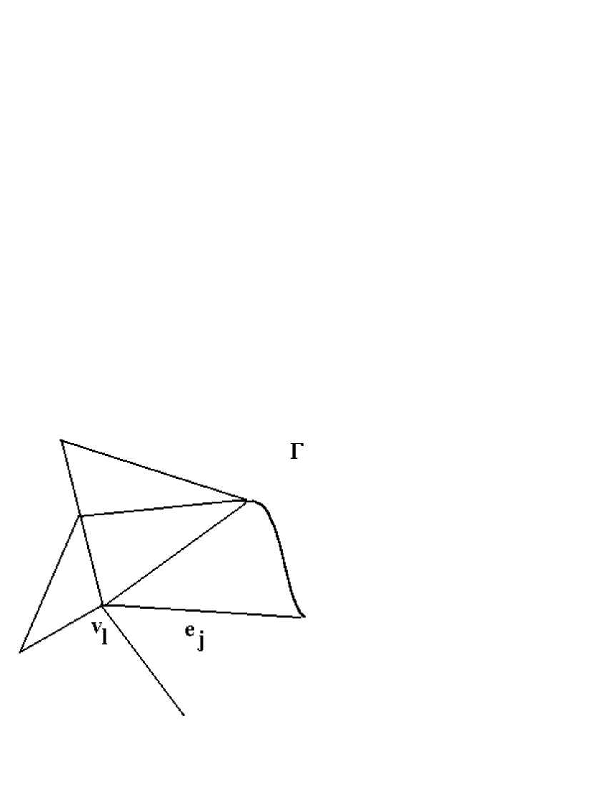
Figure 1: Graph $\Gamma$.

The reader should notice that the points of a metric graph are not only its vertices, as it is normally assumed in the combinatorial setting, but all intermediate points $x$ on the edges as well. So, while a function on a combinatorial graph is defined on the set $V$ of its vertices, functions $f(x)$ on a quantum graph $\Gamma$ are defined along the edges (including the vertices). One can naturally define the Lebesgue measure $dx$ on the graph.

We will sometimes assume that a root vertex $o$ is singled out (the results will not depend on the choice of the root). If this is done, one can define a “norm” $\rho(x)$ of a point $x$ as

$$\rho(x)=\rho(o,x).$$

This allows us to define for any $r\geq 0$ the ball $B_{r}$ of radius $r$:

$$B_{r}=\{x\in\Gamma\,|\,\rho(x)\leq r\}.$$

The last step that is needed to finish the definition of a quantum graph is to introduce a differential Hamiltonian on $\Gamma$. The operators of interest in the simplest cases are the second arc length derivative

$$f(x)\rightarrow-\frac{d^{2}f}{dx^{2}},$$ (1)

or a more general Schrödinger operator

$$f(x)\rightarrow\left(\frac{1}{i}\frac{d}{dx}-A(x)\right)^{2}f(x)+V(x)f(x).$$ (2)

Here $x$ denotes the coordinate $x_{e}$ along each edge $e$.

Higher order differential and even pseudo-differential operators arise as well (e.g., the survey [25] and references therein). We, however, will concentrate here on second order differential operators only.

In order for the definition of these self-adjoint Hamiltonians operators to be complete, one needs to describe their domains. For reasonable classes of potentials (e.g., measurable and bounded), the natural conditions require that $f$ belongs to the Sobolev space $H^{2}(e)$ on each edge $e$. One, however clearly also needs to impose boundary value conditions at the vertices. These have been studied and described completely using both the standard extension theory of symmetric operators, as well as symplectic geometry approach [11, 16, 19, 26, 32, 33, 34]. The simplest one is the so called Neumann condition

$$\begin{cases}f&\mbox{ is continuous at each vertex }v\\ \sum\limits_{v\in e}\frac{df}{dx_{e}}(v)=0&\mbox{ at each vertex }v\end{cases}$$ (3)

3 Schnol-Bloch theorems

Schnol type theorems in PDEs ([40], see also [8, 15, 22, 41]) treat the following question. If there exists a non-zero $L_{2}$-solution of the equation $Hu=\lambda u$, then clearly $\lambda$ is a point of the point spectrum of $H$. Is there a similar test for detecting that $\lambda$ belongs to the whole spectrum? Imagine that one has a solution (a generalized eigenfunction) of a self-adjoint equation $Hu=\lambda u$ and that one has some control of the growth of this solution (e.g., it is bounded). When can one guarantee that $\lambda$ is a point of the spectrum of $H$? For the Schrödinger equation in $\mathbb{R}^{n}$ with a potential bounded from below, the standard Schnol theorem [8, 15, 40] says that existence of a sub-exponentially growing solution implies that $\lambda\in\sigma(H)$. A version of this theorem is known in solid state physics as the Bloch theorem [1, 22, 38]: if $H$ is a periodic Schrödinger operator, then existence of a bounded eigenfunction corresponding to a point $\lambda$ guarantees that $\lambda\in\sigma(H)$. On the other hand, for the hyperbolic plane Laplace-Beltrami operator $\Delta_{H}$, there is an infinite dimensional space of bounded solutions of $\Delta_{H}u=0$. Indeed, using the Poincaré unit disk model of the hyperbolic plane, one has $\Delta_{H}=(1-|z|^{2})^{2}\Delta$, where $\Delta$ is the Euclidean Laplacian (e.g., Section 4 of the Introduction in [17], or any other book on hyperbolic geometry). Thus, all bounded harmonic functions $u$ on the unit disk (which form an infinite-dimensional space) satisfy the equation $\Delta_{H}u=0$. However, the point $0$ is still not in the spectrum of $\Delta_{H}$ (e.g., [31]). This happens due to the exponential growth of the volume of the hyperbolic ball of radius $r$. A similar Schnol type theorem here would need to request some decay of the generalized eigenfunction. The purpose of this section is establishing a Schnol-Bloch type theorem for graphs.

Let $\Gamma$ be a rooted connected infinite quantum graph satisfying the condition A and equipped with the Hamiltonian $-\dfrac{d^{2}}{dx^{2}}$ and any self-adjoint vertex conditions.

Theorem 2.

(A Schnol type theorem) Let the graph $\Gamma$ satisfy the above conditions and $\lambda\in\mathbb{R}$. If there exists a function $\phi(x)$ on $\Gamma$ that belongs to the Sobolev space $H^{2}$ on each edge, satisfies all vertex conditions, the equation

$$-\frac{d^{2}\phi}{dx^{2}}=\lambda\phi\mbox{ for a.e. }x\in\Gamma,$$ (4)

and the sub-exponential growth condition

$$\int\limits_{B_{r}}|\phi(x)|^{2}dx\leq C_{\epsilon}e^{\epsilon r}$$ (5)

for any $\epsilon>0$, then $\lambda\in\sigma(H)$.

This theorem implies in particular the following

Corollary 3.

(A Bloch type theorem.) Let the graph $\Gamma$ satisfy conditions of the Theorem and be of a sub-exponential growth (i.e., the volume of $B_{r}$ grows sub-exponentially). If there exists a bounded solution of the equation (4), then $\lambda\in\sigma(H)$.

Simple examples show that existence of a bounded solution does not guarantee that $\lambda\in\sigma(H)$, if the graph is of exponential growth (i.e., a regular tree of degree 3 or higher).

Proof of Theorem 2. Let us define for any $r>0$ the following compact subset $\Gamma_{r}$ of the graph: it consists of all points of the edges with both ends in $B_{r}$. The following inclusions hold:

$$\Gamma_{r-L}\subset B_{r}\subset\Gamma_{r+L}.$$ (6)

We hence conclude that the integral sub-exponential growth condition (5) holds if one replaces $B_{r}$ by $\Gamma_{r}$. Let us introduce the function

$$J(r):=\int\limits_{\Gamma_{r}}|\phi(x)|^{2}dx.$$ (7)

Given an $\epsilon>0$, one can find a sequence $r_{k}\to\infty$ such that

$$J(r_{k}+L)\leq e^{\epsilon}J(r_{k}),$$

otherwise one gets a contradiction with the sub-exponential growth condition. We remind to the reader that each set $\Gamma_{r}$ consists of complete edges only.

Let $\theta(x)$ be any smooth function on $[0,l_{0}/4]$ such that it is identically equal to $1$ in a neighborhood of $0$ and identically equal to zero close to $l_{0}/4$. Here $l_{0}$ is the lower bound for the lengths of all edges of $\Gamma$, which was assumed to be strictly positive. We define a cut-off function $\theta_{k}$ on $\Gamma$. It is equal to $1$ on $\Gamma_{r_{k}}$ and to $0$ on all edges which do not have vertices in $\Gamma_{r_{k}}$. We only need to define it along the edges that have exactly one vertex in $\Gamma_{r_{k}}$. Let $e$ be an edge whose one vertex $v$ is contained in $\Gamma_{r_{k}}$. The function $\theta_{k}$ is defined to be equal to $1$ along $e$ starting from $v$ till the middle of the edge, then it is continued by an appropriately shifted copy of $\theta(x)$ (which by construction will become zero at least at the distance $l_{e}/4$ from the end of the edge), and stays zero after that. Notice that due to the construction, any derivative of the functions $\theta_{k}(x)$ is uniformly bounded with respect to $k$ and $x\in\Gamma$. Besides, these functions are identically equal to $1$ or $0$ around any vertex.

We can now construct a sequence of approximate eigenfunctions $\phi_{k}(x)$ of the operator $H$ as follows:

$$\phi_{k}(x)=\theta_{k}(x)\phi(x).$$

One can notice that the functions $\phi_{k}(x)$ satisfy the same boundary conditions that $\phi$ did, since the factors $\theta_{k}$ are identically equal to $1$ or $0$ around the vertices. This implies that $\phi_{k}(x)$ belongs to the domain of $H$ in $L^{2}(\Gamma)$. Besides, we clearly have

$$\|\phi_{k}\|^{2}\geq J(r_{k}).$$ (8)

One also notices that the functions $\phi_{k}$ are supported in $\Gamma_{r_{k}+L}$.

Let us now apply $H-\lambda$ to these test functions:

$$(H-\lambda)\phi_{k}=\theta_{k}\left(-\phi^{\prime\prime}-\lambda\phi\right)-2\theta_{k}^{\prime}\phi^{\prime}-\theta_{k}^{\prime\prime}\phi=-2\theta_{k}^{\prime}\phi^{\prime}-\theta_{k}^{\prime\prime}.$$ (9)

We have used here that $\phi$ satisfies (4).

Using the properties of the cut-off functions $\theta_{k}$, one gets

$$\|(H-\lambda)\phi_{k}\|^{2}\leq C\int\limits_{x\in\mbox{ supp }\theta_{k}^{\prime}}\left(|\phi(x)|^{2}+|\phi^{\prime}(x)|^{2}\right)dx.$$ (10)

Since the supports of the derivatives $\theta_{k}^{\prime}$ belong to the interiors of the edges and are at a qualified distance from the vertices, we have standard Schauder estimates for

$$\int\limits_{x\in\mbox{ supp }\theta_{k}^{\prime}}|\phi^{\prime}(x)|^{2}dx$$

by for instance the integral

$$\int\limits_{\rho(x)\in[r_{k}+\frac{l_{0}}{4},r_{k}+L-\frac{l_{0}}{4}]}|\phi(x)|^{2}dx.$$

This leads to the estimate

$$\begin{array}[]{c}\|(H-\lambda)\phi_{k}\|^{2}\leq C\int\limits_{\rho(x)\in[r_{k}+\frac{l_{0}}{4},r_{k}+L-\frac{l_{0}}{4}]}|\phi(x)|^{2}dx\\ \leq C(J(r_{k}+L)-J(r_{k}))\leq C(e^{\epsilon}-1)J(r_{k})\leq C(e^{\epsilon}-1)\|\phi_{k}\|^{2},\end{array}$$ (11)

where the constant $C$ does not depend on $k,\epsilon$. Since $\epsilon>0$ was arbitrary, we conclude that $\lambda\in\sigma(H)$. ∎

Remark 4.

1. If one has a generalized eigenfunction that satisfies (5) for some fixed $\epsilon$, rather than arbitrary one as in the theorem, one cannot conclude that $\lambda\in\sigma(H)$. However, it is easy to modify the proof to estimate from above its distance $\mbox{dist}(\lambda,\sigma(H))$ to the spectrum, which when $\epsilon\to 0$ will reproduce the statement of the theorem.

2. The same result holds for more general Hamiltonian, e.g. for Schrödinger operators $-\dfrac{d^{2}}{dx^{2}}+q(x)$ with bounded from below potentials $q(x)\geq q_{0}>-\infty$ and any self-adjoint vertex conditions.

3. Analogous results, with essentially the same (a little bit simpler) proofs hold for discrete operators on infinite combinatorial graphs as well. One can notice then the relation of the Schnol type theorems to the amenability properties of discrete groups and graphs (e.g., the Følner condition) and to the notion of infinite Ramanujan graphs.

   The author will provide details concerning these remarks elsewhere.

4 Spectral gaps created by graph decorations

Existence of spectral gaps is known to be one of the spectral features of high interest in the various fields ranging from solid state physics to photonic crystal theory, to waveguides, to theory of discrete groups and graphs. A standard way of trying to create spectral gaps is to make a medium periodic (e.g., [1, 22, 23, 38]). This is why most of photonic crystal structures that are being created are periodic. However, periodicity neither guarantees existence of gaps (except in the $1D$ case), nor it allows any easy control of gap locations or sizes, nor it is a unique way to achieve spectral gaps. It has been noticed by several researchers (the first such references known to the author are [35, 36]), that spreading small geometric scatterers throughout the medium (not necessarily in a periodic fashion) might lead to spectral gaps as well. This has been confirmed on quantum graph models in [2, 9], and finally made very clear and precise in the case of combinatorial graphs in [39]. It was proposed in [39] that a simple procedure of “decorating” a graph leads to a very much controllable gap structure. We will show here that up to some caveat, the same procedure works in the case of quantum graphs. Let us describe the decoration procedure of [39] adopted to the quantum graph situation.

Let $\Gamma_{0}$ be a quantum graph satisfying the condition A and such that the corresponding Hamiltonian is the negative second derivative along the edges with the Neumann conditions (3) at the vertices. Let also $\Gamma_{1}$ be a finite connected quantum graph with the same type of the Hamiltonian, with any self-adjoint vertex conditions. The graph $\Gamma_{1}$ will be our “decoration.” We assume that a root vertex $v_{1}$ is singled out in $\Gamma_{1}$. The decoration procedure works as follows: The new graph $\Gamma$ is obtained by attaching a copy of $\Gamma_{1}$ to each vertex $v$ of $\Gamma_{0}$ and identifying $v_{1}$ with $v$ (see Fig. 2).

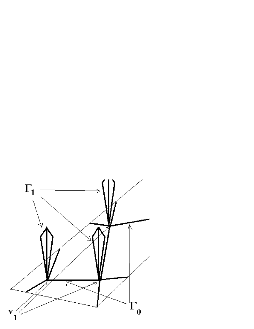
Figure 2: Decoration of a quantum graph $\Gamma_{0}$ by $\Gamma_{1}$.

Notice that there is a natural embedding $\Gamma_{0}\subset\Gamma$. We will denote by $V,V_{0}$, and $V_{1}$ the vertices sets of $\Gamma,\Gamma_{0}$, and $\Gamma_{1}$ correspondingly. The Hamiltonian $H$ on $\Gamma$ is defined as the negative second derivative on each edge, with the Neumann conditions at each vertex of $\Gamma_{0}$ (including the former $v_{1}$ vertices of the decorations) and the initially assumed conditions on $V_{1}\backslash v_{1}$, repeated on each attached copy of the decoration.

Dirichlet eigenvalues of each edge (which are clearly directly related to the edge lengths spectrum) often play an exceptional role in quantum graph considerations (see the discussions below). Let $\{l_{j}\}$ be the lengths of the edges of the original graph $\Gamma_{0}$. Then we define the Dirichlet spectrum $\sigma_{D}$ of $\Gamma_{0}$ as the closure of the set

$$\mathop{\cup}\limits_{n\in(\mathbb{Z}\backslash 0),j}\{\pi^{2}n^{2}/l_{j}^{2}\}\subset\mathbb{R}.$$

If the graph $\Gamma_{0}$ is finite, no closure is required.

Let us also define the operator $H_{1}$ on the decoration graph $\Gamma_{1}$ that acts as the negative second derivative on each edge and satisfies the self-adjoint conditions assumed before on $V_{1}\backslash v_{1}$ and zero Dirichlet condition at $v_{1}$.

We can now state the result of this section, which was previously announced in [24, 27]. The conditions of the theorem can be weakened, but we consider for brevity the simplest case here, which seems already rather useful.

Theorem 5.

Let $\lambda_{0}\in\mathbb{R}\backslash\sigma_{D}$ be a simple eigenvalue of $H_{1}$ with the eigenfunction $\psi$ such that the sum of the derivatives of $\psi$ at $v_{1}$ along all outgoing edges is not zero. Then there is a punctured neighborhood of $\lambda_{0}$ that does not belong to the spectrum $\sigma(H)$ of $\Gamma$.

Proof.

We will prove here the theorem for the case of a finite graph $\Gamma_{0}$ only. The case of an infinite graph is a little bit more technical and will be considered elsewhere. The proof consists of removing the decorations and replacing them by altered vertex conditions. This is done simultaneously and the same way at each vertex $v\in V_{0}\subset V$, so we will describe it for one vertex $v$, which will be identified with $v_{1}\in\Gamma_{1}$.

Let us define a function that we will call Dirichlet-to-Neumann function $\Lambda(\lambda)$ for $\Gamma_{1}$. It is defined in a punctured neighborhood of $\lambda_{0}$ not intersecting $\sigma_{D}$ as follows. If $\lambda\neq\lambda_{0}$ is a regular point of $H_{1}$, one can uniquely solve the problem

$${\begin{cases}-u^{\prime\prime}=\lambda u\mbox{ on each edge of }\Gamma_{1}\\ u\mbox{ satisfies the prescribed boundary conditions on }V_{1}\backslash v_{1}\\ u(v_{1})=1\end{cases}}$$ (12)

We denote by $\Lambda(\lambda)$ the sum of the outgoing derivatives of the solution $u(x)$ at the vertex $v_{1}$.

Lemma 6.

Under the conditions of the Theorem, the Dirichlet-to-Neumann function $\Lambda(\lambda)$ is analytic in a punctured neighborhood of $\lambda_{0}$, with a first order pole (with non-zero residue) at $\lambda_{0}$.

Proof of the lemma. Let $\psi$ be the eigenfunction of $H_{1}$ assumed in the statement of the theorem. We denote by $\Psi\neq 0$ the sum of outgoing derivatives of $\psi$ at $v_{1}$. Let also $f$ be a function on $\Gamma_{1}$ defined as follows: it is supported in a small neighborhood of the vertex $v_{1}$ (so small that it does not contain other vertices of $\Gamma_{1}$), is equal to $1$ near $v_{1}$, and is smooth inside the edges. We also denote by $R_{H_{1}}(\lambda)=(H_{1}-\lambda)^{-1}$ the resolvent of $H_{1}$. Then we can represent the solution $u$ of (12) as $\tilde{u}+f$, where

$$\begin{array}[]{c}\tilde{u}=-R_{H_{1}}(\lambda)(-f^{\prime\prime}-\lambda f)\\ =-(\lambda-\lambda_{0})^{-1}<-f^{\prime\prime}-\lambda f,\psi>_{L_{2}(\Gamma)}\psi(x)+A(\lambda)\\ =-(\lambda-\lambda_{0})^{-1}\Psi\psi(x)+A(\lambda).\\ \end{array}$$

Here $A(\lambda)$ is analytic in a neighborhood of $\lambda_{0}$. Noticing that the sums of the outgoing derivatives at $v_{1}$ of both functions $u$ and $\tilde{u}$ on $\Gamma_{1}$ are the same, we see that $\Lambda(\lambda)$ has a first order pole at $\lambda_{0}$ with a non-zero residue. This proves the lemma.

Let now $\lambda_{0}$ be as in the theorem. Suppose that $u(x)$ is an eigenfunction of $H$ corresponding to an eigenvalue $\lambda$ close to $\lambda_{0}$. For any vertex $v\in V_{0}$, we can solve the equation $Hu=\lambda u$ on the decoration attached to $v$, using $u(v)$ as the Dirichlet data. Then the sum of outgoing derivatives of $u$ at $v$ along the edges of the decoration is equal to $\Lambda(\lambda)u(v)$. Hence, the eigenfunction equation for $u$ on $\Gamma$ can be re-written on $\Gamma_{0}$ solely as follows:

$$\begin{cases}-u^{\prime\prime}=\lambda u\mbox{ on each edge of }\Gamma_{0}\\ u\mbox{ is continuous at all vertices }v\in V_{0}\\ \sum\limits_{v\in e}\frac{du}{dx_{e}}(v)=-\Lambda(\lambda)u(v).\end{cases}$$ (13)

We will show now that (13) is impossible for a non-zero function $u$, if $\lambda$ is close to $\lambda_{0}$. Indeed, with $\lambda$ being at a positive distance from the Dirichlet spectrum $\sigma_{D}$ of all edges, standard estimates give

$$\sum\limits_{e\in\Gamma_{0}}\|u\|^{2}_{H^{2}(e)}\leq C\sum\limits_{v\in V_{0}}|u(v)|^{2}.$$ (14)

Now Sobolev trace theorem implies

$$\sum\limits_{\{e\in\Gamma_{0},v\in V_{0}|\,v\in e\}}|\frac{du}{dx_{e}}(v)|^{2}\leq C\sum\limits_{v\in V_{0}}|u(v)|^{2}.$$ (15)

Since $\Lambda(\lambda)$ has a pole at $\lambda_{0}$, for $\lambda$ and $\lambda_{0}$ sufficiently close, we get contradiction between (15) and the last equality of (13).∎

Remark 7.

1. As it was mentioned above, the proofs for the infinite case will be provided elsewhere.

2. The proof shows that the decorations attached to each vertex do not have to be the same in order to achieve spectral gaps. One only needs to guarantee a uniform blow-up of all the Dirichlet-to-Neumann functions at each vertex when $\lambda\to\lambda_{0}$. One can also provide some estimates of the size of the gap.

3. This theorem claims that spectral gaps are guaranteed to arise around the spectrum of the decoration (with the Dirichlet condition at the attachment point $v_{1}$), unless one deals with the Dirichlet spectrum of $\Gamma_{0}$. Simple examples show that on the Dirichlet spectrum one cannot guarantee a gap. For instance, if $\Gamma_{0}$ contains a cycle consisting of edges of equal (or commensurate) lengths, then the decoration procedure cannot remove the eigenvalues that correspond to the sinusoidal waves running around this loop (see Fig. 4). However, a modification of the decoration procedure works even in the presence of Dirichlet spectrum. One just needs to introduce some “fake” vertices along the edges at appropriate locations and attach the decorations at these new vertices as well. This will be described in detail elsewhere.

4. One can create gaps by a different decoration procedure rather than the one of [39] described above. Namely, instead of attaching sideways the little “flowers” (or “kites,” as they were called in [39]) as in Fig. 2, one could incorporate an internal structure into each vertex, putting a little “spider” there as shown in Fig. 3 below.

   

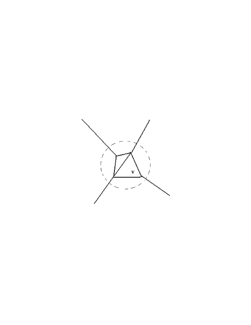
   Figure 3: A “spider” decoration.

   This graph decoration procedure was probably used explicitly for the first time in [2] (see also [9]) for the same purpose of gap creation. It will be shown elsewhere how gaps can be created using this construction (the Dirichlet spectrum plays a distinguished role there as well).

5 Bound states on periodic graphs

It is “well known” (albeit still not proven for the most general case) that elliptic periodic second order operators in $\mathbb{R}^{n}$ have no point spectrum. In fact, their spectra are absolutely continuous. In the case of Schrödinger operators with periodic electric potentials, this constituted the celebrated Thomas’ theorem [44] (see also [22, 38]). There has been a significant progress in the last decade towards proving this for the general case. One can find the description of the status of this statement for the general elliptic periodic operators in [3, 13, 23, 30]. The validity of this theorem is intimately related to the uniqueness of continuation property (that is why it fails for higher order operators), which does not hold on graphs. It is well known that bound states, and even compactly supported eigenfunctions can easily be found in combinatorial and quantum graphs, whether periodic or not. If, for instance the quantum graph has a cycle with commensurate lengths of the edges, one can easily create a sinusoidal wave supported on this loop only (see Fig. 4).

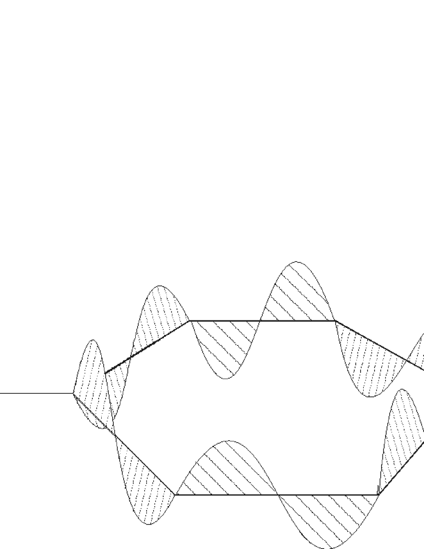
Figure 4: A loop bound state.

The question arises whether any other causes exist besides compactly supported eigenfunctions, for appearance of the pure point spectrum on periodic graphs. It has been shown previously by the author [21] that in the case of combinatorial periodic graphs, existence of bound states implies existence of the compactly supported ones. In fact, the eigenfunctions with compact support generate the whole eigenspace. We will show here that the same holds true for periodic quantum graphs as well.

One should note that point spectrum can arise for different reasons on graphs that are not periodic, e.g. on trees. For instance, one can have bound states on infinite trees with sufficiently fast growing branching number [43].

We will consider an infinite combinatorial or quantum graph $\Gamma$ with a faithful co-compact action of the free abelian group $G=\mathbb{Z}^{n}$ (i.e., the space of $G$-orbits is a compact graph).

Let us treat the combinatorial case first, so let $\Gamma$ be a combinatorial graph and $A$ a $G$-periodic finite difference (not necessarily self-adjoint) operator of a finite order acting on $l_{2}(V)$. Here, as before, $V$ is the set of vertices of $\Gamma$. The first half of the following result is proven in [21]:

Theorem 8.

If the equation $Au=0$ has a non-zero $l_{2}(V)$ solution, then it has a non-zero compactly supported solution. Moreover, the compactly supported solutions form a complete set in the space of all $l_{2}$-solutions.

Since this formulation is more complete than the one in [21], we provide its brief proof here.

Proof.

We will need to use the basic transform of Floquet theory (e.g., [22, 38]). Namely, for any compactly supported (or sufficiently fast decaying) function $u(v)$ on $V$, we define its Floquet transform

$$u(v)\mapsto\hat{u}(v,z)=\sum\limits_{g\in\mathbb{Z}^{n}}u(gv)z^{g},$$ (16)

where $gv$ denotes the action of $g\in\mathbb{Z}^{n}$ on the point $v\in V$, $z=(z_{1},...,z_{n})\in(\mathbb{C}\backslash 0)^{n}$, and $z^{g}=z_{1}^{g_{1}}\times...\times z_{n}^{g_{n}}$. We will also denote $\hat{u}(v,z)$ by $\hat{u}(z)$, where the latter expression is a function on $W$ depending on the parameter $z$. Here $W$ is a (finite) fundamental domain of the action of the group $G=\mathbb{Z}^{n}$ on $V$. Notice that images of the compactly supported functions are exactly all finite Laurent series in $z$ with coefficients in $\mathbb{C}^{|W|}$,

We will also need the unit torus

$$\mathbb{T}^{n}=\{z\in\mathbb{C}^{n}\,|\,|z_{j}|=1,j=1,...,n\}\subset\mathbb{C}^{n}.$$

It is well known and easy to establish [21, 22, 38] that the transform (16) extends to an isometry (up to a possible constant normalization factor) between $l_{2}(V)$ and $L_{2}(\mathbb{T}^{n},\mathbb{C}^{|W|})$.

After this transform, $A$ becomes the operator of multiplication in $L_{2}(\mathbb{T}^{n},\mathbb{C}^{|W|})$ by a rational $|W|\times|W|$ matrix function $A(z)$. This means that non-zero $l_{2}$-solutions of $Au=0$ are in one-to-one correspondence with $\mathbb{C}^{|W|}$-valued $L_{2}$-functions $\hat{u}$ on $\mathbb{T}^{n}$ such that $A(z)\hat{u}(z)=0$ a.e. on $\mathbb{T}^{n}$. Since we assumed that $u$, and hence $\hat{u}$ is not a zero element of $l_{2}$, we can conclude that the set of points of the torus $\mathbb{T}^{n}$ over which the matrix $A(z)$ has a non-trivial kernel, has a positive measure. On the other hand, this set in $\mathbb{C}^{n}$ is given by the algebraic equation $\det A(z)=0$ and thus is algebraic. The only way it can intersect the torus over a subset of a positive measure is that it coincides with the whole space $\mathbb{C}^{n}$. Hence, $A(z)$ has a non-zero kernel at any point $z$. Thus, its determinant is identically equal to zero. Considering this matrix over the field $\mathcal{Q}$ of rational functions, one can apply the standard linear algebra statement that claims existence of a non-zero rational solution $\phi(z)$ of $A(z)\phi(z)=0$. As indicated before, such functions before the Floquet transform were compactly supported solutions of $Au=0$. This proves the first statement of the theorem, about the existence of compactly supported eigenfunctions.

To prove completeness, we need to do a little bit more work. Let us denote by $Q_{1}(z),...,Q_{r}(z)$ a finite set of the generators of all non-zero polynomial (vector-valued) solutions of $A(z)Q(z)=0$ (it is known to exist, e.g. [18, lemma 7.6.3, Ch.VII]). Floquet transform reduces the completeness statement we need to prove to the following

Lemma 9.

Combinations

$$y(z)=\sum\limits_{j=1,..,r}a_{j}(z)Q_{j}(z),$$ (17)

where $a_{j}(z)$ are finite Laurent sums, are $L_{2}$-dense in the space of all $\mathbb{C}^{|W|}$-valued $L_{2}$-solutions of the equation

$$A(z)y(z)=0.$$ (18)

Proof of the lemma. First of all, any $L_{2}(\mathbb{T}^{n})$-function $a_{j}$ can be approximated by a finite Laurent sum. Indeed, this is done by taking finite partial sums of the Fourier series of $a_{j}$ on the torus $\mathbb{T}^{n}$. So, it is sufficient to approximate any $L_{2}$-solution $y(z)$ of (18) by sums (17) with $L_{2}$ coefficients $a_{j}$. Let $k>0$ be the minimal (over $z\in\mathbb{C}^{n}$ or $z\in\mathbb{T}^{n}$, which is the same) dimension of $KerA(z)$. The set $B\subset\mathbb{T}^{n}$ of points $z$ where $dim\,Ker\,A(z)>k$ is an algebraic variety of codimension at least $2$, and hence has zero measure on $\mathbb{T}^{n}$. Hence, it is sufficient to do $L_{2}$ approximation outside of small neighborhoods of $B$. Let $z_{0}\in\mathbb{T}^{n}\backslash B$ and $U$ be a sufficiently small neighborhood of $z_{0}$ not intersecting $B$. Then over (a complex neighborhood of) $U$ the kernels $KerA(z)$ form a trivial holomorphic vector bundle. Let $f_{l}(z)$ be a basis of holomorphic sections of this bundle. Then the portion of $y$ over $U$ can be represented as $\sum b_{l}(z)f_{l}(z)$ with $L_{2}$-functions $b_{l}$. Now, one uses [18, lemma 7.6.3, Ch. VII] again to see that sums (17) with analytic $a_{j}$ approximate the sections $f_{l}$. This proves the Lemma and hence the Theorem. ∎

The following observation is standard:

Proposition 10.

If the periodic operator $A$ is self-adjoint, then its spectrum has no singular continuous part.

Indeed, the singular continuous part is excluded for such periodic operators by the standard well known argument (e.g., [14, 44], or the proof of Theorem 4.5.9 in [22]).

Now the case of quantum graphs (at least when the Dirichlet spectrum is excluded) can be reduced to the combinatorial one, similarly to the way described in [26].

Theorem 11.

Let $\Gamma$ be a $G=\mathbb{Z}^{n}$-periodic (in the meaning already specified) quantum graph equipped with the second derivative Hamiltonian and arbitrary vertex conditions at the vertices. Then, existence of a non-zero $L_{2}$-eigenfunction corresponding to an eigenvalue $\lambda$ implies existence of a compactly supported eigenfunction, and the set of compactly supported eigenfunctions is complete in the eigenspace. If the vertex conditions are self-adjoint, the spectrum of the Hamiltonian has no singular continuous part.

Proof.

The first step is to make sure that $\lambda$ stays away from the Dirichlet spectrum $\sigma_{D}$, which in the case we consider is discrete. If by any chance $\lambda\in\sigma_{D}$, one can introduce “fake” additional vertices of degree $2$ on the edges of the fundamental domain of the graph and then repeat them periodically in such a way that the Dirichlet eigenvalues of the new shorter edges will avoid $\lambda$. If one imposes Neumann conditions at these new vertices, their introduction does not influence the operator at all. So, we can assume from the start that $\lambda$ is not in $\sigma_{D}$. Let now $F$ be an $L_{2}$-eigenfunction. Since we are away from the Dirichlet spectrum $\sigma_{D}$, resolvent and trace estimates analogous to the ones in the proof of the previous theorem show that the vector $f=\{F(v)\}$ of the vertex values belongs to $l_{2}(V)$ if and only if $F\in\L_{2}(\Gamma)$. Since $\lambda$ is not in $\sigma_{D}$, solving the boundary value problem for the eigenfunction equation $HF=\lambda F$ on each edge separately in terms of the boundary values of $F$, we can express the derivatives of $F$ at each vertex in terms of its vertex values $f$ solely. Thus, boundary conditions (which involve the values of $F$ and of its vertex derivatives) lead to a periodic finite order difference equation $Af=0$ on the combinatorial counterpart of the quantum graph. Theorem 8 claims existence and completeness of combinatorial compactly supported solutions. Reversing the procedure (which is possible since we are not on the Dirichlet spectrum), we conclude existence and completeness of compactly supported eigenfunctions of the quantum graph.

The part about the absence of singular continuous spectrum is standard (as for the combinatorial graphs). ∎

Remark 12.

Compactly supported eigenfunctions on graphs are sometimes called “scars.”

6 Acknowledgment

The author thanks M. Aizenman, R. Carlson, P. Exner, R. Grigorchuk, S. Novikov, H. Schenck, J. Schenker, and R. Schrader for relevant information and M. Solomyak and the reviewers for useful comments about the manuscript.

This research was partly sponsored by the NSF through the Grants DMS 9610444, 0072248, 0296150, and 0406022. The author expresses his gratitude to NSF for this support. The content of this paper does not necessarily reflect the position or the policy of the federal government, and no official endorsement should be inferred.

References

- [1] N.W. Ashcroft and N.D.Mermin, Solid State Physics, Holt, Rinehart and Winston, New York-London, 1976.
- [2] J. Avron, P. Exner, and Y. Last, Periodic Schrödinger operators with large gaps and Wannier-Stark ladders, Phys. Rev. Lett. 72(1994), 869-899.
- [3] M. Sh. Birman and T. A. Suslina, A periodic magnetic Hamiltonian with a variable metric. The problem of absolute continuity, Algebra i Analiz 11(1999), no.2. English translation in St. Petersburg Math J. 11(2000), no.2 203-232.
- [4] F. Chung, Spectral Graph Theory, Amer. Math. Soc., Providence R.I., 1997.
- [5] Y. Colin de Verdière, Spectres De Graphes, Societe Mathematique De France, 1998
- [6] D. Cvetkovic, M. Doob, and H. Sachs, Spectra of Graphs, Acad. Press., NY 1979.
- [7] D. Cvetkovic, M. Doob, I. Gutman, A. Targasev, Recent Results in the Theory of Graph Spectra, Ann. Disc. Math. 36, North Holland, 1988.
- [8] H.L. Cycon, R.G. Froese, W. Kirsch, and B. Simon, Schro dinger Operators with Applications to Quantum Mechanics and Global Geometry, Texts and Monographs in Physics, Springer Verlag, Berlin 1987.
- [9] P. Exner, Lattice Kronig-Penney models, Phys. Rev. Lett. 74 (1995), 3503-3506
- [10] P. Exner and P. Šeba, Electrons in semiconductor microstructures: a challenge to operator theorists, in Schrödinger Operators, Standard and Nonstandard (Dubna 1988)., World Scientific, Singapore 1989; pp. 79-100.
- [11] P. Exner, P. Šeba, Free quantum motion on a branching graph, Rep. Math. Phys. 28 (1989), 7-26
- [12] A. Figotin and P. Kuchment, Spectral properties of classical waves in high contrast periodic media, SIAM J. Appl. Math. 58(1998), no.2, 683-702.
- [13] L. Friedlander, On the spectrum of a class of second order periodic elliptic differential operators, Comm. Partial Diff. Equat. 15(1990), 1631–1647.
- [14] C. Gerard and F. Nier, The Mourre theory for analytically fibered operators, J. Funct. Anal. 152(1998), no.1, 202-219.
- [15] I. M. Glazman, Direct Methods of Qualitative Spectral Analysis of Singular Differential Operators, Isr. Progr. Sci. Transl., Jerusalem 1965.
- [16] M. Harmer, Hermitian symplectic geometry and extension theory, J. Phys. A: Math. Gen. 33(2000), 9193-9203
- [17] S. Helgason, Groups and Geometric Analysis, Academic Press 1984.
- [18] L. Hörmander, “An Introduction to Complex Analysis in Several Variables”, Van Nostrand, Princeton, NJ 1966.
- [19] V. Kostrykin and R. Schrader, Kirchhoff’s rule for quantum wires, J. Phys. A 32(1999), 595-630.
- [20] T. Kottos and U. Smilansky, Quantum chaos on graphs, Phys. Rev. Lett. 79(1997), 4794–4797.
- [21] P. Kuchment, To the Floquet theory of periodic difference equations, in Geometrical and Algebraical Aspects in Several Complex Variables, C. Berenstein and D. Struppa (Eds.), Cetraro (Italy), June 1989, EditEl, 1991, 203-209.
- [22] P. Kuchment, Floquet Theory for Partial Differential Equations, Birkhäuser, Basel 1993.
- [23] P. Kuchment, The Mathematics of Photonics Crystals, Ch. 7 in Mathematical Modeling in Optical Science, Bao, G., Cowsar, L. and Masters, W.(Editors), 207–272, Philadelphia: SIAM, 2001.
- [24] P. Kuchment, Differential and pseudo-differential operators on graphs as models of mesoscopic systems, in Analysis and Applications, H. Begehr, R. Gilbert, and M. W. Wang (Editors), Kluwer Acad. Publ. 2003, 7-30.
- [25] P. Kuchment, Graph models of wave propagation in thin structures, Waves in Random Media 12(2002), no. 4, R1-R24.
- [26] P. Kuchment, Quantum graphs I. Some basic structures, Waves in Random media, 14 (2004), S107–S128.
- [27] P. Kuchment, On some spectral problems of mathematical physics, in Partial Differential Equations and Inverse Problems, C. Conca, R. Manasevich, G. Uhlmann, and M. S. Vogelius (Editors), Contemp. Math. v. 362, 2004.
- [28] P. Kuchment and L. Kunyansky, Spectral Properties of High Contrast Band-Gap Materials and Operators on Graphs, Experimental Mathematics, 8(1999), no.1, 1-28.
- [29] P. Kuchment and L. Kunyansky, Differential operators on graphs and photonic crystals, Adv. Comput. Math. 16(2002), 263-290.
- [30] P. Kuchment and S. Levendorskii, On the structure of spectra of periodic elliptic operators, Trans. AMS 354 (2002), 537-569.
- [31] S. Lang, , Springer-Verlag, NY 1985.
- [32] S.Novikov, Schrödinger operators on graphs and topology, Russian Math Surveys, 52(1997), no. 6, 177-178.
- [33] S.Novikov, Discrete Schrödinger operators and topology, Asian Math. J., 2(1999), no. 4, 841-853.
- [34] S.Novikov, Schrödinger operators on graphs and symplectic geometry, The Arnoldfest (Toronto, ON, 1997), 397–413, Fields Inst. Commun., 24, Amer. Math. Soc., Providence, RI, 1999.
- [35] B. S. Pavlov, A model of zero-radius potential with internal structure, Theor. Math. Phys. 59(1984), 544-580.
- [36] B. S. Pavlov, The theory of extensions and explicitly solvable models, Russian. Math. Surveys 42(1987), 127-168.
- [37] Quantum Graphs and Their Applications, P. Kuchment (Editor), special issue of Waves in Random Media 14 (2004), no. 1.
- [38] M. Reed and B. Simon, Methods of Modern Mathematical Physics v. 4, Acad. Press, NY 1978.
- [39] J. Schenker and M. Aizenman, The creation of spectral gaps by graph decoration, Lett. Math. Phys. 53 (2000), no. 3, 253.
- [40] E. Schnol , On the behavior of eigenfunctions of the Schrödinger equation, Mat. Sbornik 42 (1957), 273–286.
- [41] M. A. Shubin, Spectral theory of elliptic operators on non-compact manifolds, Methodes semi-classiques, v. I (Nantes, 1990), Asterisque 207(1992), no. 5, 35–108.
- [42] M.A. Shubin, Spectral theory of elliptic operators on non-compact manifolds: qualitative results, Spectral Theory and Geometry (Edinburgh, 1998), 226–283, London Math. Soc. Lect. Ser., 273, Cambridge Univ. Press, Cambridge 1999.
- [43] M. Solomyak, On the spectrum of the Laplacian on regular metric trees, Waves in Random Media, 14 (2004), no. 1, S155–S171.
- [44] L. E. Thomas, Time dependent approach to scattering from impurities in a crystal, Comm. Math. Phys. 33(1973), 335-343.