Virtual turning points and bifurcation of Stokes curves for higher order ordinary differential equations

Abstract

For a higher order linear ordinary differential operator $P$, its Stokes curve bifurcates in general when it hits another turning point of $P$. This phenomenon is most neatly understandable by taking into account Stokes curves emanating from virtual turning points, together with those from ordinary turning points. This understanding of the bifurcation of a Stokes curve plays an important role in resolving a paradox recently found in the Noumi-Yamada system, a system of linear differential equations associated with the fourth Painlevé equation.

As is pointed out by Silverstone 1 , notorious ambiguities in the connection problems in WKB theory are resolved if we make use of the Borel resummation method; in a word, we have to first specify the region (the so-called Stokes region) where the Borel sum of a WKB solution is well-defined. The importance of the Borel resummation in WKB analysis is also shown from several viewpoints by Bender-Wu, Voros, Zinn-Justin and others 2 . In the description of the Stokes region for a second order linear ordinary differential operator $P=P(x,\eta^{-1}d/dx)=P(x,\eta^{-1}\xi)$ with a large parameter $\eta$ we need to consider only Stokes curves emanating from turning points, that is, the union of an integral curve of the direction field

$${\rm Im}(\xi_{j}(x)-\xi_{k}(x))dx=0$$ (1)

that emanates from a point a satisfying

$$\xi_{j}(a)=\xi_{k}(a)$$ (2)

where $\xi_{j}(x)$ and $\xi_{k}(x)$ are characteristic roots of the operator $P$. For higher order operators, however, the totality of Stokes curves emanating from turning points (i.e., points satisfying (2)) does not suffice to describe the Stokes region as Berk et al. 3 first pointed out; we need a “new Stokes curve” that does not emanate from a turning point in the complete description of the Stokes region. Later three of the ${\rm authors}$ 4 noticed that a new Stokes curve is an ordinary Stokes curve (i.e., an integral curve of (1)) that emanates from a virtual turning point, which is defined through the Borel transform $P_{B}$ of the operator $P$, i.e., $P_{B}=P(x,\partial_{x}/\partial_{y})$. For example, let us consider the following third order operator $P$ 3 :

$$P=\eta^{-3}\frac{d^{3}}{dx^{3}}+3\eta^{-1}\frac{d}{dx}+2ix\qquad(\eta\gg 1)$$ (3)

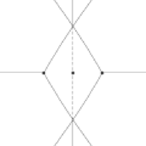
Figure 1: Stokes geometry for the operator given by (3).

With an appropriate labeling of the characteristic root $\xi_{j}(x)$ of the equation

$$\xi^{3}+3\xi+2ix=0$$ (4)

we find Fig. 1 of Stokes geometry of $P$; in Fig. 1, the point $x=-1$ (resp., $+1$) is an ordinary turning point determined by $\xi_{1}(x)=\xi_{2}(x)$ (resp., $\xi_{2}(x)=\xi_{3}(x)$), the point $x=0$ is the virtual turning point detected by Ref. 4 ; it satisfies

$$\int^{x}_{-1}\xi_{1}(x)dx=\int^{1}_{-1}\xi_{2}(x)dx+\int^{x}_{1}\xi_{3}(x)dx.$$ (5)

The Stokes curve defined by the direction field ${\rm Im}(\xi_{1}(x)-\xi_{3}(x))dx=0$ that emanates from $x=0$ coincides with the new Stokes curve detected in Ref. 3 . No Stokes phenomena occur on the dotted portion of the curve in Fig. 1 (3 , 4 ). See 4b for an application to the Landau-Zener type level crossing problem of the notion of virtual turning points and Stokes curves emanating from them.

Figure 2: Stokes geometry of (3) with (a) $\textrm{arg}\eta=(\frac{1}{2}-\frac{1}{12})\pi$, (b) $\textrm{arg}\eta=\pi/2$ and (c) $\textrm{arg}\eta=(\frac{1}{2}+\frac{1}{12})\pi$.

By changing $\textrm{arg}\eta$ in Eq.(3), we find the Stokes geometry for (a) $\textrm{arg}\eta=(\frac{1}{2}-\frac{1}{12})\pi$, (b) $\textrm{arg}\eta=\pi/2$ and (c) $\textrm{arg}\eta=(\frac{1}{2}+\frac{1}{12})\pi$ respectively in Fig. 2 (a), (b) and (c). Note that the virtual turning point is invariant when $\textrm{arg}\eta$ is changed, just like an ordinary turning point is so. One then observes in Fig. 2 (a) and (c) the interchange of the relative location of a Stokes curve emanating from an ordinary turning point and that emanating from a virtual turning point. One also finds that the bifurcation of a Stokes curve in Fig. 2 (b) should look awkward if the Stokes curves emanating from the virtual turning point were not included in Fig. 2 (a), (c). Since the bifurcation of the Stokes curve in Fig. 2 (b) is a consequence of the (square-root type) singularity of $\xi_{2}(x)$ at $x=\pm 1$, bifurcation of a Stokes curve of this kind is a rather universal phenomenon. Actually when a Stokes curve hits a simple turning point with a change of a parameter, the Stokes curve bifurcates as in Fig. 3(b). Fig. 3(a) and (c) respectively show the configuration of two simple turning points $s_{1},s_{2}$, a virtual turning point $v$ and Stokes curves emanating from them before and after the hitting. See 7a for the concrete computation in the example of the Stokes geometry for the quantized Hénon map.

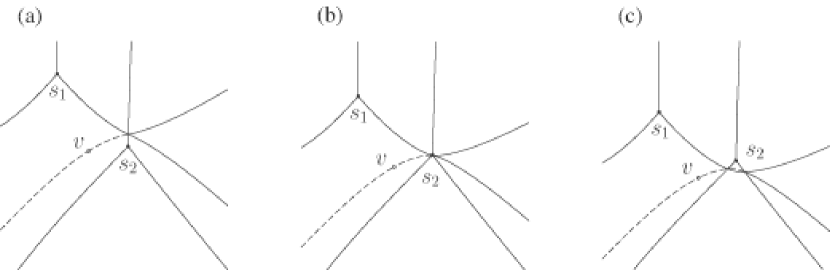
Figure 3: Schematic picture of bifurcation of the Stokes curve.

The relevance of virtual turning points and bifurcation of Stokes curve so far described has turned out to bear substantially important practical meaning in the exact WKB analysis (i.e., WKB analysis based on the Borel resummation) of the Painlevé hierarchy of Noumi-Yamada type 5 ; its first member consists of the symmetric form of the fourth Painlevé equation 6

$$\eta^{-1}\frac{df_{j}}{dt}=f_{j}(f_{j+1}-f_{j+2})+\alpha_{j}\quad(j=0,1,2)$$ (6)

with $$f_{j}=f_{j-3}\quad(j=3,4)\quad\mbox{and}\quad\alpha_{0}+\alpha_{1}+\alpha_{2}=\eta^{-1},$$

and its underlying “Schrödinger” equation

$$-\eta^{-1}x\frac{\partial}{\partial x}\begin{pmatrix}\psi_{0}\\ \psi_{1}\\ \psi_{2}\end{pmatrix}=\begin{pmatrix}(2\alpha_{1}+\alpha_{2})/3&f_{1}&1\\ x&(-\alpha_{1}+\alpha_{2})/3&f_{2}\\ xf_{0}&x&-(\alpha_{1}+2\alpha_{2})/3\end{pmatrix}\begin{pmatrix}\psi_{0}\\ \psi_{1}\\ \psi_{2}\end{pmatrix}$$ (7)

together with its appropriate deformation equation omitted here.

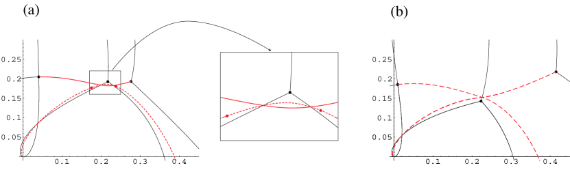
Figure 4: Fig. 4(a) shows the relevant part of the Stokes geometry of (7) when $t$ lies on a portion of a Stokes curve that contains its starting turning point and Fig. 4(b) shows that for $t$ lying on the Stokes curve but far away from the turning point. For the clarity of the presentation we use the following convention: A black (resp. red) dot indicates an ordinary (resp. a virtual) turning point. A black (resp. red) solid line indicates a Stokes curve emanating from an ordinary turning points (resp. doubly overlapped Stokes curves from ordinary turning points) and a red dotted (resp. dashed) line indicates a Stokes curve from a virtual turning point sitting on a Stokes curve from another virtual (resp. ordinary) turning point.

A computer-assisted study 7 of the Stokes geometry of (7) shows that its expected degeneracy, i.e., the appearance of a Stokes curve connecting two turning points is not observed when the parameter $t$ enters on a some portion of a Stokes curve of (6) if we take into account only ordinary turning points; this contradicts with the result 8 obtained for the same fourth Painlevé equation but with a different underlying Schrödinger equation of the second order. The paradoxical situation is resolved if both ordinary and virtual turning points are taken into consideration. To illustrate the situation we show the following Fig. 4; In Figure 4(b) the ordinary simple turning point is connected with a virtual turning point by a Stokes curve and the ordinary double turning point is connected with another virtual turning point.

The point is that a Stokes curve hits a turning point in the Stokes geometry of (7) at some point $t=t_{*}$ on the Stokes curve of (6) and that the role of an ordinary turning point and that of a virtual turning point are switched there through the mechanism we found in Fig. 3.

More complicated topological changes of configurations of Stokes curves and turning points, both ordinary and virtual, will be reported elsewhere 7a , 7 ; they are basically attained by repeated applications of the mechanism observed in Fig. 3.