Abstract

An elementary introduction is given to the subject of Supersymmetry in Quantum Mechanics which can be understood and appreciated by any one who has taken a first course in quantum mechanics. We demonstrate with explicit examples that given a solvable problem in quantum mechanics with n bound states, one can construct new exactly solvable n Hamiltonians having n-1,n-2,…,0 bound states. The relationship between the eigenvalues, eigenfunctions and scattering matrix of the supersymmetric partner potentials is derived and a class of reflectionless potentials are explicitly constructed. We extend the operator method of solving the one-dimensional harmonic oscillator problem to a class of potentials called shape invariant potentials. It is worth emphasizing that this class includes almost all the solvable problems that are found in the standard text books on quantum mechanics. Further, we show that given any potential with at least one bound state, one can very easily construct one continuous parameter family of potentials having same eigenvalues and s-matrix. The supersymmetry inspired WKB approximation (SWKB) is also discussed and it is shown that unlike the usual WKB, the lowest order SWKB approximation is exact for the shape invariant potentials and further, this approximation is not only exact for large quantum numbers but by construction, it is also exact for the ground state. Finally, we also construct new exactly solvable periodic potentials by using the machinery of supersymmetric quantum mechanics.

1 Introduction

Supersymmetry (SUSY) is a symmetry between fermions and bosons. It was first introduced in High Energy Physics in an attempt to obtain a unified description of all basic interactions of nature. It is a highly unusual symmetry since fermions and bosons have very different properties. For example, while identical bosons condense, in view of Pauli exclusion principle, no two identical fermions can occupy the same state! Thus it is quite remarkable that one could implement such a symmetry. The algebra involved in SUSY is a graded Lie algebra which closes under a combination of commutation and anti-commutation relations. In the context of particle physics, SUSY predicts that corresponding to every basic constituent of nature, there should be a supersymmetric partner with spin differing by half-integral unit. Further it predicts that the two supersymmetric partners must have identical mass in case supersymmetry is a good symmetry of nature. In the context of unified theory for the basic interactions of nature, supersymmetry predicts the existence of SUSY partners of all the basic constituents of nature, i.e. SUSY partners of 6 quarks, 6 leptons and the corresponding gauge quanta (8 gluons, photon, $Z^{0},W^{\pm}$). The fact that no scalar electron has been experimentally observed with mass less than about 100 GeV (while the electron mass is only 0.5 MeV) means that SUSY must be a badly broken symmetry of nature. Once this realization came, people started to understand the difficult question of spontaneous SUSY breaking in quantum field theories. It is in this context that Witten[1] suggested in 1981 that perhaps one should first understand the question of SUSY breaking in the simpler setting of nonrelativistic quantum mechanics and this is how the area of SUSY quantum mechanics was born.

Once people started studying various aspects of supersymmetric quantum mechanics (SQM), it was soon clear that this field was interesting in its own right, not just as a model for testing concepts of SUSY field theories. In the last 20 years, SQM has given us deep insight into several aspects of standard nonrelativistic quantum mechanics. The purpose of these lectures is to give a brief introduction to some of these ideas. For example,

1. It is well known that the infinite square well is one of the simplest exactly solvable problem in nonrelativistic QM and the energy eigenvalues are given by $E_{n}=c(n+1)^{2}$ with $c$ being a constant. Are there other potentials for which the energy eigenvalues have a similar form and is there a simple way of obtaining these potentials.

2. Free particle is obviously the simplest (and in a way trivial) example in QM with no bound states, no reflection, and the transmission probability being unity. Are there some nontrivial potentials for which also there is no reflection and is it possible to easily construct them?

3. Among the large number of possible potentials, only a very few are analytically solvable. What is so special about these “solvable” potentials?

4. One problem which all of us solve by two different methods (i.e. by directly solving Schrödinger equation and by operator method) is the one dimensional harmonic oscillator potential. Can one extend this operator method to a class of potentials? In this context, it is worth recalling that the operator method of solving the one dimensional harmonic oscillator problem is very fundamental and in fact forms the basis of quantum field theory as well as many body theory.

5. Given a potential $V(x)$, the corresponding energy eigenvalues $E_{n}$, and the scattering matrix (i.e. the reflection and transmission coefficients $R(k),T(k)$ in the one dimensional case or the phase shifts in the three dimensional case) are unique. Is the converse also true, i.e. given all the energy eigenvalues and $R(k)$ and $T(k)$ at all energies, is the corresponding potential unique? If not, then how does one construct these strictly isospectral potentials having same $E_{n},R(k),T(k)$?

6. A related question is about the construction of the soliton solutions of the KdV and other nonlinear equations. Can these be easily constructed from the formalism of SQM?

7. WKB is one of the celebrated semiclassical approximation scheme which is expected to be exact for large quantum numbers but usually is not as good for small quantum numbers. Is it possible to have a modified scheme which by construction would not only be exact for large quantum numbers but even for the ground state so that it has a chance to do better even when the quantum numbers are neither too large nor too small? Further, the lowest order WKB is exact in the case of only two potentials, i.e. the one dimensional oscillator and the Morse potentials. Can one construct a modified WKB scheme for which the lowest order approximation will be exact for a class of potentials?

The purpose of these lectures is to answer some of the questions raised above. We shall first discuss the basic formalism of SQM and then discuss some of these issues. For pedagogical reason, we have kept these lectures at an elementary level. More details as well as discussion about several other topics can be obtained from our book [2] and Physics Reports [3] on this subject. A clarification is in order here. Unlike in SUSY quantum field theory, in SQM, supersymmetric partners are not fermions and bosons, instead here, SUSY relates the eigenstates and S-matrix of the two partner Hamiltonians.

2 Formalism

Let us consider the operators

$$A={\hbar\over\sqrt{2m}}{d\over dx}+W(x)~{},~{}A^{{\dagger}}={-\hbar\over\sqrt{2m}}{d\over dx}+W(x)~{}.$$ (1)

From these two operators, we can construct two Hamiltonians $H_{1},H_{2}$ given by

$$H_{1}=A^{{\dagger}}A\,,~{}~{}H_{2}=AA^{{\dagger}}\,.$$ (2)

It is easily checked that

$$H_{1}=-\frac{\hbar^{2}}{2m}\frac{d^{2}}{dx^{2}}+V_{1}(x)\,,~{}~{}~{}V_{1}(x)=W^{2}(x)-{\hbar\over\sqrt{2m}}W^{\prime}(x)\,,$$ (3)

$$H_{2}=-\frac{\hbar^{2}}{2m}\frac{d^{2}}{dx^{2}}+V_{2}(x)\,,~{}~{}~{}V_{2}(x)=W^{2}(x)+{\hbar\over\sqrt{2m}}W^{\prime}(x)\,,$$ (4)

The quantity $W(x)$ is generally referred to as the superpotential in SUSY QM literature while $V_{1,2}(x)$ are termed as the supersymmetric partner potentials.

As we shall see, the energy eigenvalues, the wave functions and the S-matrices of $H_{1}$ and $H_{2}$ are related. In particular, we shall show that if $E$ is the eigenvalue of $H_{1}$ then it is also the eigenvalue of $H_{2}$ and vice a versa. To that end notice that the energy eigenvalues of both $H_{1}$ and $H_{2}$ are positive semi-definite ($E_{n}^{(1,2)}\geq 0$) . Further, the Schrödinger equation for $H_{1}$ is

$$H_{1}\psi_{n}^{(1)}=A^{{\dagger}}A\psi_{n}^{(1)}=E_{n}^{(1)}\psi_{n}^{(1)}\,.$$ (5)

On multiplying both sides of this equation by the operator $A$ from the left, we get

$$H_{2}(A\psi_{n}^{(1)})=AA^{{\dagger}}A\psi_{n}^{(1)}=E_{n}^{(1)}(A\psi_{n}^{(1)})~{}.$$ (6)

Similarly, the Schrödinger equation for $H_{2}$

$$H_{2}\psi_{n}^{(2)}=AA^{{\dagger}}\psi_{n}^{(2)}=E_{n}^{(2)}\psi_{n}^{(2)}$$ (7)

implies

$$H_{1}(A^{{\dagger}}\psi_{n}^{(2)})=A^{{\dagger}}AA^{{\dagger}}\psi_{n}^{(2)}=E_{n}^{(2)}(A^{{\dagger}}\psi_{n}^{(2)})~{}.$$ (8)

Thus we have shown that if $E$ is an eigenvalue of the Hamiltonian $H_{1}(H_{2})$ with eigenfunction $\psi$, then same $E$ is also the eigenvalue of the Hamiltonian $H_{2}(H_{1})$ and the corresponding eigenfunction is $A\psi(A^{{\dagger}}\psi)$.

The above proof breaks down in case $A\psi_{0}^{(1)}=0$, i.e. when the ground state is annihilated by the operator $A$ (note that the spectrum of both the Hamiltonians is nonnegative). Thus the exact relationship between the eigenstates of the two Hamiltonians will crucially depend on if $A\psi_{0}^{(1)}$ is zero or nonzero, i.e. if the ground state energy $E_{0}^{(1)}$ is zero or nonzero.

$A\psi_{0}^{(1)}\neq 0$: In this case the proof goes through for all the states including the ground state and hence all the eigenstates of the two Hamiltonians are paired, i.e. they are related by ($n=0,1,2,...$)

$$E_{n}^{(2)}=E_{n}^{(1)}>0\,,$$ (9)

$$\psi_{n}^{(2)}=[E_{n}^{(1)}]^{-1/2}A\psi_{n}^{(1)}~{},$$ (10)

$$\psi_{n}^{(1)}=[E_{n}^{(2)}]^{-1/2}A^{{\dagger}}\psi_{n}^{(2)}~{}.$$ (11)

$A\psi_{0}^{(1)}=0$: In this case, $E_{0}^{(1)}=0$ and this state is unpaired while all other states of the two Hamiltonian are paired. It is then clear that the eigenvalues and eigenfunctions of the two Hamiltonians $H_{1}$ and $H_{2}$ are related by $(n=0,1,2,...)$

$$E_{n}^{(2)}=E_{n+1}^{(1)},\hskip 14.45377ptE_{0}^{(1)}=0~{},$$ (12)

$$\psi_{n}^{(2)}=[E_{n+1}^{(1)}]^{-1/2}A\psi_{n+1}^{(1)}~{},$$ (13)

$$\psi_{n+1}^{(1)}=[E_{n}^{(2)}]^{-1/2}A^{{\dagger}}\psi_{n}^{(2)}~{}.$$ (14)

The equation $A\psi_{0}^{(1)}=0$ can be interpreted in the following two different ways depending on whether the superpotential $W(x)$ or the ground state wave function $\psi_{0}^{(1)}$ is known. In case $W(x)$ is known then one can solve the equation $A\psi_{0}^{(1)}=0$ by using eq. (1) and the ground state wavefunction of $H_{1}$ is given, in terms of the superpotential $W$ by

$$\psi_{0}^{(1)}=N\exp[-\frac{\sqrt{2m}}{\hbar}\int^{x}W(y)dy]\,.$$ (15)

Instead, if $\psi_{0}^{(1)}$ is known, then this equation gives us the superpotential $W$, i.e.

$$W(x)=-\frac{\hbar}{\sqrt{2m}}\frac{\psi_{0}^{\prime(1)}(x)}{\psi_{0}^{(1)}(x)}$$ (16)

Several Comments are in order at this stage.

1. Notice that if $\psi_{n+1}^{(1)}$ ( $\psi_{n}^{(2)}$) of $H_{1}$ ($H_{2}$) is normalized then the wave function $\psi_{n}^{(2)}$ ($\psi_{n+1}^{(1)}$) is also normalized. Similar remarks are obviously also valid for eigenfunctions in eqs. (10) and (11).

2. The operator $A$ ($A^{{\dagger}}$) not only converts an eigenfunction of $H_{1}(H_{2})$ into an eigenfunction of $H_{2}(H_{1})$ with the same energy, but it also destroys (creates) an extra node in the eigenfunction.

3. Note that since the bound state wave functions must vanish at $x=\pm\infty$ (or at the two ends) hence it is clear from eq. (15) that $A\psi_{0}^{(1)}=0$ and $A^{{\dagger}}\psi_{0}^{(2)}=0$ can never be satisfied simultaneously and hence only one of the two ground state energies can be zero. As a matter of convention we shall always choose $W$ in such a way that only $\psi_{0}^{(1)}$ (if at all) is normalized so that $E_{0}^{(2)}>0$ (notice that $E_{0}^{(2)}=0$ requires that $A^{{\dagger}}\psi_{0}^{(2)}=0$, see eq. (7)).

4. In case $A\psi_{0}^{(1)}=0$, since the ground state wave function of $H_{1}$ is annihilated by the operator $A$, this state has no SUSY partner. Thus knowing all the eigenfunctions of $H_{1}$ we can determine the eigenfunctions of $H_{2}$ using the operator $A$, and vice versa using $A^{{\dagger}}$ we can reconstruct all the eigenfunctions of $H_{1}$ from those of $H_{2}$ except for the ground state. This is illustrated in Fig. 1.

   

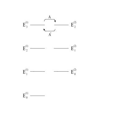
   Figure 1: Energy levels of two (unbroken) supersymmetric partner potentials. The action of the operators $A$ and $A^{\dagger}$ are displayed. The levels are degenerate except that $V_{1}$ has an extra state at zero energy.

The underlying reason for the degeneracy of the spectra of $H_{1}$ and $H_{2}$ can be understood most easily from the properties of the SUSY algebra. That is we can consider a matrix SUSY Hamiltonian of the form

$$H=\left[\matrix{H_{1}&0\cr 0&H_{2}\cr}\right]$$ (17)

which contains both $H_{1}$ and $H_{2}$. This matrix Hamiltonian is part of a closed algebra which contains both bosonic and fermionic operators with commutation and anti-commutation relations. We consider the operators

$$Q=\left[\matrix{0&0\cr A&0\cr}\right],~{}~{}~{}Q^{{\dagger}}=\left[\matrix{0&A^{{\dagger}}\cr 0&0\cr}\right]$$ (18)

in conjunction with $H$. The following commutation and anticommutation relations then describe the closed superalgebra $sl(1/1)$:

$$[H,Q] = [H,Q^{{\dagger}}]=0~{},$$

$$\{Q,Q^{{\dagger}}\} = H~{}~{},\hskip 14.45377pt\{Q,Q\}=\{Q^{{\dagger}},Q^{{\dagger}}\}=0~{}.$$ (19)

The fact that the supercharges $Q$ and $Q^{{\dagger}}$ commute with $H$ is responsible for the degeneracy in the spectra of $H_{1}$ and $H_{2}$.

Let us now try to understand as to when is SUSY spontaneously broken and when does it remain unbroken. In this context, let us recall that a symmetry of the Hamiltonian (or Lagrangian) can be spontaneously broken if the lowest energy solution does not respect that symmetry, as for example in a ferromagnet, where rotational invariance of the Hamiltonian is broken by the ground state. We can define the ground state in our system by a two dimensional column vector:

$$\psi_{0}=\left[\matrix{\psi_{0}^{(1)}\cr\psi_{0}^{(2)}\cr}\right]\,.$$ (20)

Then it is easily checked that in case $A\psi_{0}^{(1)}\neq 0$ then $Q\psi_{0}\neq 0$, $Q^{{\dagger}}\psi_{0}\neq 0$ and so SUSY is spontaneously broken while if $A\psi_{0}^{(1)}=0$ then $Q\psi_{0}=0,Q^{{\dagger}}\psi_{0}=0$ and SUSY remains unbroken. Unless stated otherwise, throughout these lectures we shall be discussing the case when SUSY remains unbroken.

Summarizing, we thus see that when SUSY is unbroken, then starting from an exactly solvable potential $V(x)$ with $n$ bound states and ground state energy $E_{0}$, one has $V_{1}(x)=V(x)-E_{0}$ whose ground state energy is therefore 0 by construction. Using the above formalism, one can then immediately obtain all the $n-1$ eigenstates of $H_{2}$. One can now start from the exactly solvable Hamiltonian $H_{2}$ and obtain all the $n-2$ eigenstates of $H_{3}$. In this way, by starting from an exactly solvable problem with $n$ bound states, one can construct new $n$ exactly solvable potentials $H_{2},H_{3},...,H_{n+1}$ with $n-1,n-2,...,0$ bound states.

Illustration: Let us look at a well known potential, namely the infinite square well and determine its SUSY partner potential. Consider a particle of mass $m$ in an infinite square well potential of width $L$

$$V(x) = 0,\hskip 36.135pt0\leq x\leq L~{},$$ (21)

$$= \infty,\hskip 36.135pt-\infty<x<0~{},x>L~{}.$$

The normalized ground state wave function is known to be

$$\psi_{0}^{(1)}=(2/L)^{1/2}\sin(\pi x/L),\hskip 21.68121pt0\leq x\leq L~{},$$ (22)

and the ground state energy is

$$E_{0}={\hbar^{2}\pi^{2}\over 2mL^{2}}\,.$$ (23)

Subtracting off the ground state energy so that the Hamiltonian can be factorized, the energy eigenvalues of $H_{1}$ = $H-E_{0}$ are

$$E_{n}^{(1)}={n(n+2)\over 2mL^{2}}\hbar^{2}\pi^{2}\,,\ n=0,1,2,...\,,$$ (24)

and the normalized eigenfunctions of $H_{1}$ are (the same as those of $H$), i.e.

$$\psi_{n}^{(1)}=(2/L)^{1/2}\sin{(n+1)\pi x\over L}~{},\hskip 36.135pt0\leq x\leq L~{}.$$ (25)

The superpotential for this problem is readily obtained using eqs. (16) and (22)

$$W(x)=-{\hbar\over\sqrt{2m}}{\pi\over L}{\rm cot}(\pi x/L)$$ (26)

and hence the supersymmetric partner potential $V_{2}$ is

$$V_{2}(x)={\hbar^{2}\pi^{2}\over 2mL^{2}}[2~{}{\rm cosec}^{2}(\pi x/L)-1]~{}.$$ (27)

The wave functions for $H_{2}$ are obtained by applying the operator $A$ to the wave functions of $H_{1}$. In particular we find that the normalized ground and first excited state wave functions are

$$\psi_{0}^{(2)}=-2\sqrt{\frac{2}{3L}}\sin^{2}(\pi x/L),\hskip 21.68121pt\psi_{1}^{(2)}=-\frac{2}{\sqrt{L}}\sin(\pi x/L)\sin(2\pi x/L)~{}.$$ (28)

Thus we have shown using SUSY that two rather different potentials corresponding to $H_{1}$ and $H_{2}$ have exactly the same spectra except for the fact that $H_{2}$ has one fewer bound state. In Fig. 2

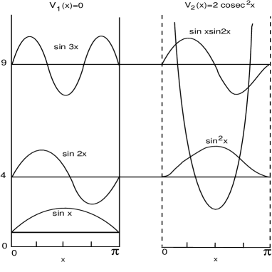
Figure 2: The infinite square well potential $V=0$ of width $\pi$ and its partner potential $V=2~{}\rm{cosec}^{2}x$ in units $\hbar=2m=1$

we show the supersymmetric partner potentials $V_{1}$ and $V_{2}$ and the first few eigenfunctions. For convenience we have chosen $L=\pi$ and $\hbar=2m=1$.

We can now start from $H_{2}$ and using its ground state wavefunction as given by eq. (28), the corresponding superpotential turns out to be

$$W_{2}(x)=-{\hbar\over\sqrt{2m}}{2\pi\over L}{\rm cot}(\pi x/L)\,,$$ (29)

and hence the partner potential $V_{3}(x)$ turns out to be

$$V_{3}(x)={\hbar^{2}\pi^{2}\over 2mL^{2}}[6~{}{\rm cosec}^{2}(\pi x/L)-4]~{}.$$ (30)

Using the above superpotential $W_{2}$, the ground state wavefunction of $V_{3}(x)$ is easily computed by using eq. (13)

$$\psi_{0}^{(3)}(x)~{}\propto~{}\sin^{3}(\pi x/L)\,.$$ (31)

In this way one can construct one (discrete) parameter family of potentials given by ($p=0,1,2,...$)

$$V_{p+1}(x)={\hbar^{2}\pi^{2}\over 2mL^{2}}[p(p+1)~{}{\rm cosec}^{2}(\pi x/L)-p^{2}],$$ (32)

and it is easily seen that its spectrum is given by

$$E_{n}^{(p+1)}=n(n+2p+2)\,,~{}~{}n=0,1,2,...\,,$$ (33)

while its eigenfunctions can be easily derived recursively from those of infinite-square well. For example, its ground state wave function is

$$\psi_{0}^{(p+1)}~{}\propto~{}\sin^{(p+1)}(\pi x/L)\,.$$ (34)

In this way we have shown, how to generate a whole class of new solvable potentials by starting from an analytically solvable problem.

So far, we have explicitly included all factors like $\hbar,m$ etc. However, from now onward, for simplicity (unless stated otherwise), we shall work in units where $\hbar=1,2m=1$.

Scattering: Supersymmetry also allows one to relate the reflection and transmission coefficients in situations where the two partner potentials have continuous spectra. In order for scattering to take place in both of the partner potentials, it is necessary that the potentials $V_{1,2}$ are finite as $x\rightarrow-\infty$ or as $x\rightarrow+\infty$ or both. Let us define

$$W(x\rightarrow\pm\infty)\equiv W_{\pm}~{}.$$ (35)

Then it follows that

$$V_{1,2}\rightarrow W_{\pm}^{2}\hskip 36.135pt{\rm as}\hskip 7.22743ptx\rightarrow\pm\infty\,.$$ (36)

Let us consider an incident plane wave $e^{ikx}$ of energy $E$ coming from the direction $x\rightarrow-\infty$. As a result of scattering from the potentials $V_{1,2}(x)$ one would obtain transmitted waves $T_{1,2}(k)e^{ik^{\prime}x}$ and reflected waves $R_{1,2}(k)e^{-ikx}$. Thus we have

$$\psi^{(1,2)}(k,x\rightarrow-\infty) \rightarrow e^{ikx}+R_{1,2}e^{-ikx}~{},$$

$$\psi^{(1,2)}(k^{\prime},x\rightarrow+\infty) \rightarrow T_{1,2}e^{ik^{\prime}x}~{},$$ (37)

where $k$ and $k^{\prime}$ are given by

$$k=(E-W_{-}^{2})^{1/2}~{},\hskip 14.45377ptk^{\prime}=(E-W_{+}^{2})^{1/2}~{}.$$ (38)

SUSY connects continuum wave functions of $H_{1}$ and $H_{2}$ having the same energy analogously to what happens in the discrete spectrum. Thus using eqs. (13) and (14) we have the relationships:

$$e^{ikx}+R_{1}e^{-ikx} = N[(-ik+W_{-})e^{ikx}+(ik+W_{-})e^{-ikx}R_{2}]~{},$$

$$T_{1}e^{ik^{\prime}x} = N[(-ik^{\prime}+W_{+})e^{ik^{\prime}x}T_{2}]~{},$$ (39)

where $N$ is an overall normalization constant. On equating terms with the same exponent and eliminating $N$, we find:

$$R_{1}(k) = \left({W_{-}+ik\over W_{-}-ik}\right)R_{2}(k)~{},$$

$$T_{1}(k) = \left({W_{+}-ik^{\prime}\over W_{-}-ik}\right)T_{2}(k)~{}.$$ (40)

A few remarks are in order at this stage.
(1) Clearly $|R_{1}|^{2}=|R_{2}|^{2}$ and $|T_{1}|^{2}=|T_{2}|^{2}$, that is the partner potentials have identical reflection and transmission probabilities.
(2) $R_{1}(T_{1})$ and $R_{2}(T_{2})$ have the same poles in the complex plane except that $R_{1}(T_{1})$ has an extra pole at $k=-iW_{-}$. This pole is on the positive imaginary axis only if $W_{-}<0$ in which case it corresponds to a zero energy bound state.
(3) In the special case that $W_{+}=W_{-}$, we have that $T_{1}(k)=T_{2}(k)$.
(4) When $W_{-}=0$ then $R_{1}(k)=-R_{2}(k)$.
(5) For symmetric potentials, $W_{+}=-W_{-}$, and hence $k=k^{\prime}$ so that the relation between $T_{1}$ and $T_{2}$ is the same as that between $R_{1}$ and $R_{2}$, i.e. $R_{1}(k)/R_{2}(k)=T_{1}(k)/T_{2}(k)$.

Reflectionless Potentials: It is clear from these remarks that if one of the partner potentials is a constant potential (i.e. a free particle), then the other partner will be of necessity reflectionless. In this way we can understand the reflectionless potentials of the form $V(x)=n(n+1)~{}{{\rm sech}}^{2}x$ which play a critical role in understanding the soliton solutions of the Korteweg-de Vries (KdV) equation. Let us consider the superpotential

$$W(x)=B\ \rm{tanh}~{}x~{}.$$ (41)

The two partner potentials are

$$V_{1} = B^{2}-B\ (B+1)\rm{sech}^{2}x~{},$$

$$V_{2} = B^{2}-B(B-1)\rm{sech}^{2}~{}x~{}.$$ (42)

We see that for $B=1$, $V_{2}(x)$ corresponds to a constant potential (free particle) with no bound states, transmission coefficient $T_{2}(k)=1$ and $R_{2}(k)=0$. Hence the corresponding $V_{1}$ is a reflectionless potential with precisely one bound state at $E_{0}^{(1)}=0$. Further by using eq. (2) it follows that its transmission coefficient is given by

$$T_{1}(k,B=1)=\frac{(1-ik)}{(-1-ik)}~{}.$$ (43)

If instead we choose $B=2$ then one finds that $V_{1}=4-6\rm{sech}^{2}x$, while as seen above, $V_{2}=4-2\rm{sech}^{2}x$ is reflectionless potential with one bound state! Hence it follows that $V_{1}$ must be a reflectionless potential with two bound states and using the SUSY machinery (eqs. (12) to (15)), we can immediately obtain the two eigenvalues of $V_{1}$ and the corresponding eigenfunctions. They are

$$E_{0}^{(1)}(B=2)=0\,,~{}~{}\psi_{0}^{(1)}~{}\propto\rm{sech}^{2}x\,,$$ (44)

$$E_{1}^{(1)}(B=2)=3\,,~{}~{}\psi_{1}^{(1)}~{}\propto\rm{sech}x\,\tanh x\,.$$ (45)

Further using eqs. (2) and (43) one can show that its transmission amplitude is given by

$$T_{1}(k,B=2)=\frac{(2-ik)(1-ik)}{(-2-ik)(-1-ik)}~{}.$$ (46)

Generalization to arbitrary integer $B$ is now straight forward, i.e. by choosing $B=3,4,...$, it is then easy to see that the one (discrete) parameter family of reflectionless potentials is given by ($p=1,2,3,...$)

$$V_{1}(x,B=p)=p(p+1)\rm{sech}^{2}x-p^{2}\,,$$ (47)

having $p$ bound states whose energy eigenvalues and eigenfunctions can be recursively obtained by starting from free particle and using the SUSY machinery. For example, its ground state energy is zero while the ground and first excited state eigenfunctions are

$$\psi_{0}^{(1)}(x,B=p)~{}\propto~{}{\rm sech}^{p}x\,,~{}~{}\psi_{1}^{(1)}(x,B=p)~{}\propto~{}{\rm sech}^{p-1}x\,\tanh x\,.$$ (48)

Further, its transmission coefficient is given by

$$T_{1}(k,p)=\frac{(p-ik)(p-1-ik)...(1-ik)}{(-p-ik)(-p+1-ik)...(-1-ik)}=\frac{\Gamma(-p-ik)\Gamma(p+1-ik)}{\Gamma(-ik)\Gamma(1-ik)}\,.$$ (49)

SUSY in n-dimensions: So far we have discussed SUSY QM on the full line $(-\infty\leq x\leq\infty)$. Many of these results have analogs for the $n$-dimensional potentials with spherical symmetry. For example, for spherically symmetric potentials in three dimensions one can make a partial wave expansion in terms of the wave functions:

$$\psi_{nlm}(r,\theta,\phi)={1\over r}R_{nl}(r)Y_{lm}(\theta,\phi)~{}.$$ (50)

Then it is easily shown that the reduced radial wave function $R_{nl}$ satisfies $(0\leq r\leq\infty)$

$$-{d^{2}R_{nl}(r)\over dr^{2}}+\biggl{[}V(r)+\frac{l(l+1)}{r^{2}}\biggr{]}R_{nl}(r)\equiv HR_{nl}(r)=ER_{nl}(r)\,.$$ (51)

Notice that this is a Schrödinger equation for an effective one dimensional potential which contains the original potential plus an angular momentum barrier.

As an illustration, let us now show how both the Coulomb and the oscillator potentials can be cast in SUSY formalism.

Oscillator Potential: It is easily seen that in case we start with

$$W(r)=\frac{\omega r}{2}-\frac{l+1}{r}\,,$$ (52)

then the two supersymmetric partner potentials are

$$V_{1}(r) = \frac{\omega^{2}r^{2}}{4}+\frac{l(l+1)}{r^{2}}-(l+3/2)\omega$$

$$V_{2}(r) = \frac{\omega^{2}r^{2}}{4}+\frac{(l+1)(l+2)}{r^{2}}-(l+1/2)\omega\,.$$ (53)

Thus we see that in the oscillator case, a given partial wave $l$ has as its SUSY partner the same oscillator potential but for the $l+1$’th partial wave. In particular, the S and P-wave oscillator potentials are the SUSY partners of each other.

Coulomb Potential: Let us start with

$$W(r)=\frac{e^{2}}{2(l+1)}-\frac{l+1}{r}\,,$$ (54)

then it is easily shown that the two supersymmetric partner potentials are

$$V_{1}(r) = \frac{e^{4}}{4(l+1)^{2}}+\frac{l(l+1)}{r^{2}}-\frac{e^{2}}{r}$$

$$V_{2}(r) = \frac{e^{4}}{4(l+1)^{2}}+\frac{(l+1)(l+2)}{r^{2}}-\frac{e^{2}}{r}$$

Thus we see that even for the Coulomb potential, a given partial wave $l$ has as its SUSY partner the same Coulomb potential but for the $l+1$’th partial wave.

As in the one dimensional case, we can also obtain the relationship between the phase-shifts for the (radial) partner potentials. The asymptotic form of the radial wave function for the $l^{\prime}$th partial wave is

$$R(r,l)\rightarrow{1\over 2k^{\prime}}[S_{l}(k^{\prime})e^{ik^{\prime}r}-(-1)^{l}e^{-ik^{\prime}r}]~{},$$ (56)

where $S_{l}$ is the scattering function for the $l^{\prime}$th partial wave, i.e. $S_{l}(k)=e^{i\delta_{l}(k)}$ and $\delta_{l}$ is the phase shift for the l’th partial wave. Proceeding exactly as in the one dimensional case (see eqs. (35) to (2)), we obtain the following relationship between the scattering functions (and hence phase shifts) for the two partner potentials

$$S^{(1)}_{l}(k^{\prime})=\left({W_{+}-ik^{\prime}\over W_{+}+ik^{\prime}}\right)S^{(2)}_{l}(k^{\prime})~{}.$$ (57)

Here $W_{+}=W(r\rightarrow\infty)$ and $k^{\prime}=\sqrt{E-W_{+}^{2}}$.

Before finishing this section, it is amusing to note that the famous problem of charged particle in a uniform magnetic field can in fact be cast in the language of SQM. Actually one can prove a stronger result. In particular, one can show that not only uniform but even for an arbitrary magnetic field, the Pauli equation in two dimensions can be cast in the SQM formalism so long as the gyromagnetic ratio $g=2$.

Let us consider the special case when the motion of the charged particle is in a plane perpendicular to the magnetic field. In this case the Pauli Hamiltonian,for $g=2$ has the form

$$H_{Pauli}=\frac{1}{2m}\sum_{i=1}^{2}(p_{i}+\frac{e}{c}A_{i})^{2}+\frac{e\hbar}{2mc}B_{3}\sigma_{3}\,.$$ (58)

One can show that in this case if we define

$$Q ={i\over\sqrt{2}}(Q^{(1)}+iQ^{(2)})~{},$$

$$Q^{(1)} ={1\over\sqrt{2}}\left[-(p_{y}+{e\over c}A_{y})\sigma_{1}+(p_{x}+{e\over c}A_{x})\sigma_{2}\right]~{},$$

$$Q^{(2)} ={1\over\sqrt{2}}\left[(p_{x}+{e\over c}A_{x})\sigma_{1}+(p_{y}+{e\over c}A_{y})\sigma_{2}\right]~{},$$ (59)

then the Hermitian supercharges $Q^{(1)},Q^{(2)}$ and $H_{Pauli}$ satisfy the SUSY algebra

$$\{Q^{(a)},Q^{(b)}\}=H_{P}\delta^{ab}~{},~{}~{}[H_{P},Q^{(a)}]=0~{},~{}~{}a,b=1,2~{}.$$ (60)

3 Shape Invariance and Solvable Potentials

Using the ideas of SUSY QM developed in the last section and an integrability condition called the shape invariance condition, we now show that the operator method for the harmonic oscillator can be generalized to the whole class of shape invariant potentials (SIP) which include essentially all the popular, analytically solvable potentials. Indeed, we shall see that for such potentials, the generalized operator method quickly yields all the bound state energy eigenvalues, eigenfunctions as well as the scattering matrix. It turns out that this approach is essentially equivalent to Schrödinger’s method of factorization [4] although the language of SUSY is more appealing.

Let us now explain precisely what one means by shape invariance. If the pair of SUSY partner potentials $V_{1,2}(x)$ as defined in eq. (3) are similar in shape and differ only in the parameters that appear in them, then they are said to be shape invariant. More precisely, if the partner potentials $V_{1,2}(x;a_{1})$ satisfy the condition[5]

$$V_{2}(x;a_{1})=V_{1}(x;a_{2})+R(a_{1})\,,$$ (61)

where $a_{1}$ is a set of parameters, $a_{2}$ is a function of $a_{1}$ (say $a_{2}=f(a_{1})$) and the remainder $R(a_{1})$ is independent of $x$, then $V_{1}(x;a_{1})$ and $V_{2}(x;a_{1})$ are said to be shape invariant. The shape invariance condition (61) is an integrability condition. Using this condition and the hierarchy of Hamiltonians discussed in the previous section, one can easily obtain the energy eigenvalues and the eigenfunctions of any SIP when SUSY is unbroken.

Let us start from the SUSY partner Hamiltonians $H_{1}$ and $H_{2}$ whose eigenvalues and eigenfunctions are related by SUSY. Further, since SUSY is unbroken we know that

$$E^{(1)}_{0}(a_{1})=0,\quad\psi^{(1)}_{0}(x;a_{1})=N\exp\left[-\int^{x}W_{1}(y;a_{1})dy\right]\,.$$ (62)

We will now show that the entire spectrum of $H_{1}$ can be very easily obtained algebraically by using the shape invariance condition (61). As a first step, let us obtain the eigenvalue and the eigenfunction of the first excited state of $H_{1}$. We start from eq. (61) and on adding kinetic energy operator to both the sides, the shape invariance condition can also be written as

$$H_{2}(x;a_{1})=H_{1}(x;a_{2})+R(a_{1})=A^{{\dagger}}(x,a_{2})A(x,a_{2})+R(a_{1})\,.$$ (63)

Since the two Hamiltonians differ by a constant, hence it is clear that all their eigenvalues must differ from each other only by that constant and further all their eigenfunctions must be proportional to each other. In particular

$$E_{0}^{(2)}(a_{1})=E_{0}^{(1)}(a_{2})+R(a_{1})\,,~{}~{}\psi_{0}^{(2)}(x,a_{1})~{}\propto~{}\psi_{0}^{(1)}(x,a_{2})\,.$$ (64)

But clearly $E_{0}^{(1)}(a_{2})=0$ so long as the corresponding ground state wave function

$$\psi_{0}^{(1)}(x,a_{2})~{}\propto~{}\exp[-\int^{x}W(y,a_{2})\,dy]\,,$$ (65)

is an acceptable ground state wave function. And hence using eqs. (64) and (12) we obtain the eigenvalue of the first excited state

$$E_{1}^{(1)}(a_{1})=E_{0}^{(2)}(a_{1})=R(a_{1})\,.$$ (66)

Similarly, using eqs. (64) and (13) we can obtain the eigenfunction of the first excited state

$$\psi_{1}^{(1)}(x,a_{1})~{}\propto~{}A^{{\dagger}}(x,a_{1})\psi_{0}^{(2)}(x,a_{1})~{}\propto~{}A^{{\dagger}}(x,a_{1})\psi_{0}^{(1)}(x,a_{2})\,.$$ (67)

This procedure is easily generalized and we can obtain the entire bound state spectrum and the corresponding eigenfunctions of $H_{1}$. To that purpose, let us construct a series of Hamiltonians $H_{s}$, $s=1,2,3$ . In particular, following the discussion of the previous section, it is clear that if $H_{1}$ has $n$ bound states then one can construct $n$ such Hamiltonians $H_{2},H_{3}\cdots H_{n+1}$ and the $p$’th Hamiltonian $H_{p}$ will have the same spectrum as $H_{1}$ except that the first $p-1$ levels of $H_{1}$ will be absent in $H_{p}$. On repeatedly using the shape invariance condition (61), it is then clear that

$$H_{s}=-{d^{2}\over dx^{2}}+V_{1}(x;a_{s})+\sum^{s-1}_{k=1}R(a_{k})\,,$$ (68)

where $a_{s}=f^{s-1}(a_{1})$ i.e. the function $f$ applied $s-1$ times. Let us compare the spectrum of $H_{s}$ and $H_{s+1}$. In view of eqs. (61) and (68) we have

$$H_{s+1}=-{d^{2}\over dx^{2}}+V_{1}(x;a_{s+1})+\sum^{s}_{k=1}R(a_{k})$$

$$=-{d^{2}\over dx^{2}}+V_{2}(x;a_{s})+\sum^{s-1}_{k=1}R(a_{k})\,.$$ (69)

Thus $H_{s}$ and $H_{s+1}$ are SUSY partner Hamiltonians and hence have identical bound state spectra except for the ground state of $H_{s}$ whose energy is

$$E^{(s)}_{0}=\sum^{s-1}_{k=1}R(a_{k})\,.$$ (70)

This follows from eq. (68) and the fact that $E^{(1)}_{0}=0$. On going back from $H_{s}$ to $H_{s-1}$ etc, we would eventually reach $H_{2}$ and $H_{1}$ whose ground state energy is zero and whose $n$’th level is coincident with the ground state of the Hamiltonian $H_{n}$. Hence the complete eigenvalue spectrum of $H_{1}$ is given by

$$E^{(1)}_{n}(a_{1})=\sum^{n}_{k=1}R(a_{k});\hskip 14.45377ptE^{(1)}_{0}(a_{1})=0\,.$$ (71)

As far as the corresponding eigenfunctions are concerned, we now show that, similar to the case of the one dimensional harmonic oscillator, the bound state wave functions $\psi^{(1)}_{n}(x;a_{1})$ for any shape invariant potential can also be easily obtained from its ground state wave function $\psi^{(1)}_{0}(x;a_{1})$ which in turn is known in terms of the superpotential. This is possible because the operators $A$ and $A^{{\dagger}}$ link up the eigenfunctions of the same energy for the SUSY partner Hamiltonians $H_{1,2}$. Let us start from the Hamiltonian $H_{s}$ as given by eq. (68) whose ground state eigenfunction is then given by $\psi^{(1)}_{0}(x;a_{s})$. On going from $H_{s}$ to $H_{s-1}$ to $H_{2}$ to $H_{1}$ and using eq. (14) we then find that the $n$’th state unnormalized, energy eigenfunction $\psi^{(1)}_{n}(x;a_{1})$ for the original Hamiltonian $H_{1}(x;a_{1})$ is given by

$$\psi^{(1)}_{n}(x;a_{1})~{}\propto~{}A^{{\dagger}}(x;a_{1})A^{{\dagger}}(x;a_{2})...A^{{\dagger}}(x;a_{n})\,\psi^{(1)}_{0}(x;a_{n+1})\,,$$ (72)

which is clearly a generalization of the operator method of constructing the energy eigenfunctions for the one dimensional harmonic oscillator.

It is often convenient to have explicit expressions for the wave functions. In that case, instead of using the above equation, it is far simpler to use the identity

$$\psi^{(1)}_{n}(x;a_{1})=A^{{\dagger}}(x;a_{1})\,\psi^{(1)}_{n-1}(x;a_{2})\,.$$ (73)

Finally, in view of the shape invariance condition (61), the relation (2) between scattering amplitudes takes a particularly simple form

$$R_{1}(k;a_{1})=\left({W_{-}(a_{1})+ik\over W_{-}(a_{1})-ik}\right)R_{1}(k;a_{2})\,,$$ (74)

$$T_{1}(k;a_{1})=\left({W_{+}(a_{1})-ik^{\prime}\over W_{-}(a_{1})-ik}\right)T_{1}(k;a_{2})\,,$$ (75)

thereby relating the reflection and transmission coefficients of the same Hamiltonian $H_{1}$ at $a_{1}$ and $a_{2}(=f(a_{1}))$.

Illustrative Examples: It may be worthwhile at this stage to illustrate this discussion with concrete examples and obtain their energy eigenvalues and eigenfunctions analytically. As a first illustration, let us consider the partner potentials $V_{1,2}\,(x,B)$ as given by eq. (2). It is easily seen that indeed these are shape invariant. In particular we observe that

$$V_{2}(x,B)=V_{1}(x,B-1)+B^{2}-(B-1)^{2}\,,$$ (76)

so that in this particular case $a_{1}=B,a_{2}=B-1$ and $R(a_{1})=B^{2}-(B-1)^{2}=a_{1}^{2}-a_{2}^{2}$. Hence, from eq. (71) it immediately follows that the complete bound state spectrum of $V_{1}(x,B)$ is given by ($n=0,1,2,...$)

$$E_{n}^{(1)}(B)=\sum_{k=1}^{n}R(a_{k})=a_{1}^{2}-a_{n+1}^{2}=B^{2}-(B-n)^{2}\,.$$ (77)

It is really remarkable that in two lines one is able to get the entire spectrum for this potential algebraically. What about the eigenfunctions? Using the superpotential as given by eq. (41) it follows that

$$\psi_{0}^{(1)}(x,B)\propto sech^{B}(x)\,.$$ (78)

Clearly, this is an acceptable wave function so long as $B$ is any positive number. On the other hand, the first excited state wavefunction is obtained by using the formula (72)

$$\psi_{1}^{(1)}(x,a_{1}=B)~{}\propto~{}A^{+}(x,B)\psi_{0}(x,a_{2}=B-1)~{}\propto~{}[-\frac{d}{dx}+B\tanh x]{\rm sech}^{B-1}x~{}\propto~{}{\rm sech}^{B-1}x\tanh x\,.$$ (79)

Proceeding in this way, one can calculate all the bound state eigenfunctions of $V_{1}(x)$.

It is worth pointing out that here $B$ is any positive number and not just an integer. Further it is also clear from here that the number of bound states is $n+1$ in case $n<B\leq n+1$. Note that only when $B$ is integer that $V_{1,2}$ are reflectionless potentials.

As a second example, it is easily checked that the Coulomb and the oscillator potentials (in fact in arbitrary number of dimensions) are also examples of shape invariant potentials. For example, it is easy to see that in the Coulomb case, the partner potentials as given by eq. (2) are shape invariant potentials (SIP) satisfying

$$V_{2}(r,l,e)=V_{1}(r,l+1,e)+[\frac{e^{4}}{4(l+1)^{2}}-\frac{e^{4}}{4(l+2)^{2}}]\,.$$ (80)

Thus in this case, $a_{1}=l,a_{2}=l+1$ and $R(a_{1})=\frac{e^{4}}{4a_{1}^{2}}-\frac{e^{4}}{4a_{2}^{2}}$ and hence the complete spectrum of $V_{1}(r,l,e)$ is given by ($n=0,1,2,...$)

$$E_{n}^{(1)}=[\frac{e^{4}}{4(l+1)^{2}}-\frac{e^{4}}{4(l+n+1)^{2}}]\,.$$ (81)

Similarly, the oscillator partner potentials (2) are SIP satisfying

$$V_{2}(r,l,\omega)=V_{1}(r,l+1,\omega)-(l+1/2)\omega+(l+5/2)\omega\,,$$ (82)

so that in this case $a_{1}=l,a_{2}=l+1$ while $R(a_{1})=2\omega$ and hence from eq. (71) it immediately follows that the entire spectrum of the oscillator potential $V_{1}(r,l,\omega)$ is given by

$$E_{n}^{(1)}=2n\omega\,,~{}~{}n=0,1,2,...\,.$$ (83)

Let us now discuss the interesting but difficult question of the classification of various solutions to the shape invariance condition (61). This is clearly an important problem because once such a classification is available, then one can discover new SIPs which are solvable by purely algebraic methods. Unfortunately, the general problem is still unsolved, only two classes of solutions have been found so far. In the first class, the parameters $a_{1}$ and $a_{2}$ are related to each other by translation $(a_{2}=a_{1}+\alpha)$.

Remarkably enough, all well known analytically solvable potentials found in most text books on nonrelativistic quantum mechanics belong to this class. In the second class, the parameters $a_{1}$ and $a_{2}$ are related to each other by scaling $(a_{2}=qa_{1})$.

3.1 Solutions Involving Translation

We shall now point out the key steps that go into the classification of SIPs in case $a_{2}=a_{1}+\alpha$. Firstly one notices the fact that the eigenvalue spectrum of the Schrödinger equation is always such that the $n$’th eigenvalue $E_{n}$ for large $n$ obeys the constraint

$$A/n^{2}\leq E_{n}\leq Bn^{2}\,,$$ (84)

where the upper bound is saturated by the infinite square well potential while the lower bound is saturated by the Coulomb potential. Thus, for any SIP, the structure of $E_{n}$ for large $n$ is expected to be of the form

$$E_{n}\sim\sum_{\alpha}C_{\alpha}n^{\alpha}~{},~{}~{}-2\leq\alpha\leq 2\,.$$ (85)

Now, since for any SIP, $E_{n}$ is given by eq. (71), it follows that if

$$R(a_{k})\sim\sum_{\beta}k^{\beta}~{},$$ (86)

then

$$-3\leq\beta\leq 1~{}.$$ (87)

How does one implement this constraint on $R(a_{k})$? While one has no rigorous answer to this question, it is easily seen that a fairly general factorizable form of $W(x;a_{1})$ which produces the above $k$-dependence in $R(a_{k})$ is given by

$$W(x;a_{1})=\sum^{n}_{i=1}[(k_{i}+c_{i})g_{i}(x)+h_{i}(x)/(k_{i}+c_{i})+f_{i}(x)]~{},$$ (88)

where

$$a_{1}=(k_{1},k_{2}...)~{},~{}~{}a_{2}=(k_{1}+\alpha,k_{2}+\beta...)~{},$$ (89)

with $c_{i},\alpha,\beta$ being constants. Note that this ansatz excludes all potentials leading to $E_{n}$ which contain fractional powers of $n$. On using the above ansatz for $W$ in the shape invariance condition eq. (61) one can obtain the conditions to be satisfied by the functions $g_{i}(x),h_{i}(x),f_{i}(x)$. One important condition is of course that only those superpotentials $W$ are admissible which give a square integrable ground state wave function.

In Table 1, we give expressions for the various shape invariant potentials $V_{1}(x)$, superpotentials $W(x)$, parameters $a_{1}$ and $a_{2}$ and the corresponding energy eigenvalues $E^{(1)}_{n}$. Except for first 3 entries of this table, $W(x+x_{0})$ is also a solution.

Table 1: Shape invariant potentials with (n=1,2) in which the parameters $a_{2}$ and $a_{1}$ are related by translation $(a_{2}=a_{1}+\beta)$. The energy eigenvalues and eigenfunctions are given in units $\hbar=2m=1$. The constants $A,B,\alpha,\omega,l$ are all taken $\geq 0$. Unless otherwise stated, the range of potentials is $-\infty\leq x\leq\infty,0\leq r\leq\infty$. For spherically symmetric potentials, the full wave function is $\varphi_{nlm}(r,\theta,\phi)=\varphi_{nl}(r)Y_{lm}(\theta,\phi)$.

Potential	$W(x)$	$V_{1}(x;a_{1})$	$a_{1}$
Shifted oscillator	$\frac{1}{2}\omega x-b$	$\frac{1}{4}\omega^{2}\left(x-\frac{2b}{\omega}\right)^{2}-\omega/2$	$\omega$
3-D oscillator	$\frac{1}{2}\omega r-\frac{(l+1)}{r}$	$\frac{1}{4}\omega^{2}r^{2}+\frac{l(l+1)}{r^{2}}-(l+3/2)\omega$	$l$
Coulomb	$\frac{e^{2}}{2(l+1)}-\frac{(l+1)}{r}$	$-\frac{e^{2}}{r}+{l(l+1)\over r^{2}}+\frac{e^{4}}{4(l+1)^{2}}$	$l$
Morse	$A-B$ exp $(-\alpha x)$	$A^{2}+B^{2}\exp(-2\alpha x)$	A
		$-2B(A+\alpha/2)\exp(-\alpha x)$
Scarf II	$A\tanh\alpha x$ + $B{\rm sech}~{}\alpha x$	$A^{2}+(B^{2}-A^{2}-A\alpha){\rm sech}^{2}\alpha x$	A
(hyperbolic)		$+B(2A+\alpha){\rm sech}~{}\alpha x\tanh\alpha x$
Rosen-Morse II	$A\tanh\alpha x+B/A$	$A^{2}+B^{2}/A^{2}-A(A+\alpha){\rm sech}^{2}\alpha x$	A
(hyperbolic)	$(B<A^{2})$	+ 2$B$ tanh $\alpha x$
Eckart	$-A\coth\alpha r+B/A$	$A^{2}+B^{2}/A^{2}-2B$ coth $\alpha r$	A
	$(B>A^{2})$	$+A(A-\alpha){\rm cosech}^{2}\alpha r$
Scarf I	$A\tan\alpha x-B\ {\rm sec}\ \alpha x$	$-A^{2}+(A^{2}+B^{2}-A\alpha){\rm sec}^{2}\alpha x$	A
(trigonometric)	$\left(-\frac{1}{2}\pi\leq\alpha x\leq\frac{1}{2}\pi\right)$	$-B(2A-\alpha)\tan\alpha x\ {\rm sec}\ \alpha x$
Pöschl-Teller	$A\coth\alpha r$ - $B$ cosech $\alpha r$	$A^{2}+(B^{2}+A^{2}+A\alpha){\rm cosech}^{2}\alpha r$	A
	$(A<B)$	$-B(2A+\alpha)$ coth $\alpha r$ cosech $\alpha r$
Rosen-Morse I	$-A$ cot $\alpha x-B/A$	$A(A-\alpha)$cosec${}^{2}\alpha x+2B$ cot $\alpha x$	A
(trigonometric)	$(0\leq\alpha x\leq\pi)$	$-A^{2}+B^{2}/A^{2}$

Note that the wave functions for the first four potentials (Hermite and Laguerre polynomials) are special cases of the confluent hypergeometric function while the rest (Jacobi polynomials) are special cases of the hypergeometric function. In the table $s_{1}=s-n+a$, $s_{2}=s-n-a$, $s_{3}=a-n-s$, $s_{4}=-(s+n+a)$.
$a_{2}$ Eigenvalue $E_{n}^{(1)}$ Variable $y$ Wave function $\psi_{n}(y)$ $\omega$ $n\omega$ $y=\sqrt{{\omega\over 2}}\left(x-\frac{2b}{\omega}\right)$ exp $\left(-\frac{1}{2}y^{2}\right)H_{n}(y)$ $l+1$ $2n\omega$ $y=\frac{1}{2}\omega r^{2}$ $y^{(l+1)/2}$ exp$\left(-\frac{1}{2}y\right)L_{n}^{l+1/2}(y)$ $l+1$ $\frac{e^{4}}{4(l+1)^{2}}-\frac{e^{4}}{4(n+l+1)^{2}}$ $y=\frac{re^{2}}{(n+l+1)}$ $y^{(l+1)}$ exp$\left(-\frac{1}{2}y\right)L_{n}^{2l+1}(y)$ $A-\alpha$ $A^{2}-(A-n\alpha)^{2}$ $y={2B\over\alpha}e^{-\alpha x}$, $y^{s-n}$ exp$\left(-\frac{1}{2}y\right)L_{n}^{2s-2n}(y)$ $s=A/\alpha$ $A-\alpha$ $A^{2}-(A-n\alpha)^{2}$ $y$ = sinh $\alpha x$, $i^{n}(1+y^{2})^{-s/2}e^{-\lambda\tan^{-1}y}$ $s=A/\alpha,\lambda=B/\alpha$ $\times P_{n}^{(i\lambda-s-1/2,-i\lambda-s-1/2)}(iy)$ $A-\alpha$ $A^{2}-(A-n\alpha)^{2}$ $y$ = tanh $\alpha x$, $(1-y)^{s_{1}/2}(1+y)^{s_{2}/2}$ $-B^{2}/(A-n\alpha)^{2}$ $s=A/\alpha,\lambda=B/\alpha^{2}$ $\times P_{n}^{(s_{1},s_{2})}(y)$ $+B^{2}/A^{2}$ $a=\lambda/(s-n)$ $A+\alpha$ $A^{2}-(A+n\alpha)^{2}$ $y$ = coth $\alpha r$, $(y-1)^{s_{3}/2}(y+1)^{s_{4}/2}$ $-B^{2}/(A+n\alpha)^{2}$ $s=A/\alpha,\lambda=B/\alpha^{2}$ $\times P_{n}^{(s_{3},s_{4})}(y)$ $+B^{2}/A^{2}$ $a=\lambda/(n+s)$ $A+\alpha$ $(A+n\alpha)^{2}-A^{2}$ $y$ = sin $\alpha r$, $(1-y)^{(s-\lambda)/2}(1+y)^{(s+\lambda)/2}$ $s=A/\alpha,\lambda=B/\alpha$ $\times P_{n}^{(s-\lambda-1/2,s+\lambda-1/2)}(y)$ $A-\alpha$ $A^{2}-(A-n\alpha)^{2}$ $y$ = cosh $\alpha r$, $(y-1)^{(\lambda-s)/2}(y+1)^{-(\lambda+s)/2}$ $s=A/\alpha,\lambda=B/\alpha$ $\times P_{n}^{(\lambda-s-1/2,-\lambda-s-1/2)}(y)$ $A+\alpha$ $(A+n\alpha)^{2}-A^{2}$ $y$ = $i$cot $\alpha x$, $(y^{2}-1)^{-(s+n)/2}$ exp $(a\alpha x)$ $-B^{2}/(A+n\alpha)^{2}$ $s=A/\alpha,\lambda=B/\alpha^{2}$ $\times P_{n}^{(-s-n+ia,-s-n-ia)}(y)$ $+B^{2}/A^{2}$ $a=\lambda/(s+n)$

Several remarks are in order at this time.

1. Throughout this section we have used the convention of $\hbar=2m=1$. It would naively appear that if we had not put $\hbar=1$, then the shape invariant potentials as given in Table 1 would all be $\hbar$-dependent. However, it is worth noting that in each and every case, the $\hbar$-dependence is only in the constant multiplying the $x$-dependent function so that in each case we can always redefine the constant multiplying the function and obtain an $\hbar$-independent potential. For example, corresponding to the superpotential given by eq. (41), let us discuss a more general potential given by

   $$W(x)=B\tanh(\alpha x+x_{0})\,,$$ (90)

   so that the corresponding $\hbar$ and $m$-dependent partner potentials are given by

   $$V_{1}(x,B)=W^{2}-\frac{\hbar}{\sqrt{2m}}\frac{dW}{dx}=B^{2}-B(B+\frac{\hbar\alpha}{\sqrt{2m}}){\rm sech}^{2}(\alpha x+x_{0})$$

   $$V_{2}(x,A)=W^{2}+\frac{\hbar}{\sqrt{2m}}\frac{dW}{dx}=B^{2}-B(B-\frac{\hbar\alpha}{\sqrt{2m}}){\rm sech}^{2}(\alpha x+x_{0})\,,$$ (91)

   which are shape invariant. On redefining

   $$B(B+\frac{\hbar\alpha}{\sqrt{2m}})=a~{};$$ (92)

   where $a$ is $\hbar$ and $m$-independent parameter, we then have a $\hbar$-independent potential $V(x)=V_{1}(x)-B^{2}=-a{\rm sech}^{2}(\alpha x+x_{0})$.

2. It may be noted that the Coulomb as well as the harmonic oscillator potentials in $n$-dimensions are also shape invariant potentials.

3. What we have shown here is that shape invariance is a sufficient condition for exact solvability. But is it also a necessary condition? The answer is clearly no. Firstly, it has been shown that the solvable Natanzon potentials are in general not shape invariant. However, for the Natanzon potentials, the energy eigenvalues and wave functions are known only implicitly. Secondly there are various methods one of which we will discuss below of finding potentials which are strictly isospectral to the SIPs. These are not SIPs but for all of these potentials, unlike the Natanzon case, the energy eigenvalues and eigenfunctions are known in a closed form.

Solutions Involving Scaling

From 1987 until 1993 it was believed that the only shape invariant potentials were those given in Table 1 and that there were no more shape invariant potentials. However, starting in 1993, a huge class of new shape invariant potentials have been discovered. It turns out that for many of these new shape invariant potentials, the parameters $a_{2}$ and $a_{1}$ are related by scaling $(a_{2}=qa_{1},0<q<1)$ rather than by translation, a choice motivated by the recent interest in $q$-deformed Lie algebras. Many of these potentials are reflectionless and have an infinite number of bound states. So far, none of these potentials have been obtained in a closed form but are obtained only in a series form.

4 Strictly Isospectral Hamiltonians and SUSY

Given any potential $V(x)$, the corresponding bound state energy eigenvalues and the reflection and transmission coefficients $T(k),R(k)$ are unique. But is the converse also true? In particular, given the entire bound state spectrum $E_{n}$ and $T(k),R(k)$ at all energies, is the potential uniquely defined? It turns out that the answer to this question is no. This is of course well known for a long time from the inverse scattering approach. In particular, it turns out that if a potential holds $n$ bound states then there exist $n$ continuous parameter family of strictly isospectral potentials (i.e. potentials having same energy eigenvalues and same reflection and transmission coefficients at all energies). These isospectral families are closely connected to multi-soliton solutions of nonlinear integrable systems.

In this section we approach this problem within the SQM formalism and show that given any potential with at least one bound state, one can very easily construct one continuous parameter family of strictly isospectral potentials having same $E_{n},R(k),T(k),solongasitsgroundstatewavefunctionisknown$. Of course this was known for a long time from inverse scattering but the Gelfand-Levitan approach to finding them is technically much more complicated than the supersymmetry approach described here.

In SQM, the inverse scattering question can be posed as follows. Once a superpotential $W(x)$ is given then the corresponding partner potentials $V_{1,2}(x)$ are unique. But is the converse also true? In particular, for a given $V_{2}(x)$ is the corresponding $W(x)$ and hence $V_{1}(x)$ unique? In other words, what are the various possible superpotentials $\hat{W}(x)$ other than $W(x)$ satisfying

$$V_{2}(x)=\hat{W}^{2}(x)+\hat{W}^{\prime}(x)~{}.$$ (93)

If there are new solutions, then one would obtain new potentials $\hat{V}_{1}(x)=\hat{W}^{2}-\hat{W}^{\prime}$ which would be isospectral to $V_{1}(x)$. To find the most general solution, let

$$\hat{W}(x)=W(x)+\phi(x)~{},$$ (94)

in eq. (93). We then find that $y(x)=\phi^{-1}(x)$ satisfies the Bernoulli equation

$$y^{\prime}(x)=1+2Wy~{},$$ (95)

whose solution is

$$\frac{1}{y(x)}=\phi(x)=\frac{d}{dx}~{}\ln[{\cal I}(x)+\lambda]~{}.$$ (96)

Here

$${\cal I}(x)\equiv\int_{-\infty}^{x}[\psi^{(1)}_{0}(x^{\prime})]^{2}\,dx^{\prime}~{},$$ (97)

$\lambda$ is a constant of integration and $\psi^{(1)}_{0}(x)$ is the normalized ground state wave function of $V_{1}(x)=W^{2}(x)-W^{\prime}(x)$. Thus the most general $\hat{W}(x)$ satisfying eq. (93) is given by

$$\hat{W}(x,\lambda)=W(x)+\frac{d}{dx}\ln[{\cal I}(x)+\lambda]~{},$$ (98)

so that the one parameter family of potentials

$$\hat{V}_{1}(x,\lambda)=\hat{W}^{2}(x)-\hat{W}^{\prime}(x)=V_{1}(x)-2\frac{d^{2}}{dx^{2}}\ln\,[{\cal I}(x)+\lambda]~{},$$ (99)

have the same SUSY partner $V_{2}(x)$.

The corresponding normalized ground state wave functions are

$$\hat{\psi}^{(1)}_{0}(x,\lambda)=\frac{\sqrt{\lambda(1+\lambda)}\,\psi^{(1)}_{0}(x)}{{\cal I}(x)+\lambda}\,,$$ (100)

while the excited state wave functions are easily obtained by using relation (14), i.e.

$$\hat{\psi}^{(1)}_{n+1}(x,\lambda)=[-\frac{d}{dx}+W(x,\lambda)]\,\psi^{(2)}_{n}(x)\,.$$ (101)

Several comments are in order at this stage.

1. Note that this family contains the original potential $V_{1}$. This corresponds to the choices $\lambda\rightarrow\pm\infty$.

2. The fact that the potentials $V_{1}(x,\lambda)$ are strictly isospectral, i.e. have same $E_{n},R(k),T(k)$ can be seen as follows. Firstly, since all of them have the same partner potential $V_{2}(x)$, hence it follows that they must have the same spectrum. Secondly, the reflection and transmission coefficients for these potentials must be related to those of $V_{2}(x)$ by the formula (2). But from eqs. (97) and (98) it is easy to show that $\hat{W(x=\pm\infty,\lambda)}=W_{\pm}$ and hence the transmission and reflection coefficients for the entire one parameter family of potentials are identical.

3. Note that while $E_{n},R(k),T(k)$ are the same for the entire family of potentials, the wave functions for all these potentials are different. As is well known from inverse scattering, a potential is uniquely fixed only when one specifies $E_{n},R(k),T(k)$ and normalization constant of one of the eigenfunction.

4. Since $\cal{I}$ varies from $0$ to $1$ hence if we choose the continuous parameter $\lambda$ so that either $\lambda>0$ or $\lambda<-1$ then we ensure that the corresponding ground state wavefunctions $\psi_{1}(x,\lambda)$ are nonsingular.

5. The one parameter family of strictly isospectral potentials $\hat{V}_{1}(x,\lambda)$ can be shown to satisfy infinite number of conserved charges $Q_{i}$ (i=1,2,3,…). Two of these are

   $$Q_{1} = \int_{-\infty}^{\infty}V(x,\lambda)~{}dx$$

   $$Q_{2} = \int_{-\infty}^{\infty}x\,V(x,\lambda)~{}dx\,,$$ (102)

   which satisfy $\frac{dQ_{1,2}}{d\lambda}=0$ as can be easily checked by using eqs. (98) to (100). The conserved charge $Q_{2}$ implies that the one continuous parameter family of potentials are such that if one plots these potentials as a function of $x$, then the area under the curve is the same for the entire family of potentials. Similarly, all the other conservation laws tighten these potentials.

To elucidate this discussion, it may be worthwhile to explicitly construct the one-parameter family of strictly isospectral potentials corresponding to the one dimensional harmonic oscillator. In this case

$$W(x)=\frac{\omega}{2}x~{},$$ (103)

so that

$$V_{1}(x)=\frac{\omega^{2}}{4}x^{2}-\frac{\omega}{2}~{}.$$ (104)

The normalized ground state eigenfunction of $V_{1}(x)$ is

$$\psi^{(1)}_{0}(x)=\left(\frac{\omega}{2\pi}\right)^{1/4}\exp(-\omega{x^{2}}/4)~{}.$$ (105)

Using eq. (97) it is now straightforward to compute the corresponding ${\cal I}(x)$. We get

$${\cal I}(x)=1-\frac{1}{2}~{}{\rm erfc}\left(\frac{\sqrt{\omega}}{2}x\right)~{};~{}{\rm erfc}(x)=\frac{2}{\sqrt{\pi}}~{}\int_{x}^{\infty}~{}e^{-t^{2}}dt~{}.$$ (106)

Using eqs. (99) and (100), one obtains the one parameter family of isospectral potentials and the corresponding wave functions. In Figs. 3 and 4 , we have plotted some of the potentials and the corresponding ground state wave functions for the case $\omega=2$.

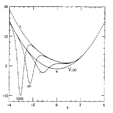
Figure 3: Selected members of the family of potentials with energy spectra identical to the one dimensional harmonic oscillator with $\omega=2$. The choice of units is $\hbar=2m=1$. The curves are labeled by the value of $\lambda$, and cover the range $0<\lambda\leq\infty$. The curve $\lambda=\infty$ is the one dimensional harmonic oscillator. The curve marked $\lambda=0$ is known as the Pursey potential and has one bound state less than the oscillator.

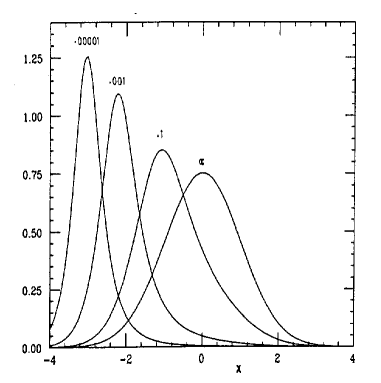
Figure 4: Ground state wave functions for all the potentials shown in Fig. 3, except the Pursey potential.

We see that as $\lambda$ decreases from $\infty$ to 0, $\hat{V}_{1}$ starts developing a minimum which shifts towards $x=-\infty$. Note that as $\lambda_{1}$ finally becomes zero this attractive potential well is lost and we lose a bound state. The remaining potential is called the Pursey potential $V_{P}(x)$. The general formula for $V_{P}(x)$ is obtained by putting $\lambda=0$ in eq. (99). An analogous situation occurs in the limit $\lambda=-1$, the remaining potential being the Abraham-Moses potential.

5 Supersymmetry Inspired WKB Approximation

We will describe here a recent extension of the semiclassical approach inspired by supersymmetry called the supersymmetric WKB (SWKB) method. It turns out that for many problems the SWKB method gives better accuracy than the WKB method. Further, we discuss and prove the remarkable result that the lowest order SWKB approximation gives exact energy eigenvalues for all SIPs with translation which include essentially all analytically solvable potentials discussed in most text books on QM. In this section we do not assume $\hbar=2m=1$ but explicitly keep all the factors of $\hbar$ and $m$.

The semiclassical WKB approximation for one dimensional potentials with two classical turning points is discussed in most quantum mechanics textbooks. The lowest order WKB quantization condition is given by ($n=0,1,2,...$)

$$\int^{x_{R}}_{x_{L}}dx\sqrt{2m[E-V(x)]}=(n+1/2)\hbar\pi\,.$$ (107)

In the special case of the one dimensional harmonic oscillator and the Morse potential, it turns out that the lowest order WKB approximation (107) is in fact exact and further, the higher order corrections are all zero.

About twenty years ago, combining the ideas of SUSY with the lowest order WKB method, the lowest order SWKB quantization condition was obtained in case SUSY is unbroken and it was shown that it yields energy eigenvalues which are not only accurate for large quantum numbers $n$ but which, by construction, are also exact for the ground state $(n=0)$. We shall now discuss the SWKB quantization in detail.

For the potential $V_{1}(x)$ corresponding to the superpotential $W(x)$, the lowest order WKB quantization condition (107) takes the form

$$\int_{x_{L}}^{x_{R}}\sqrt{2m\bigg{[}E_{n}^{(1)}-W^{2}(x)+\frac{\hbar}{\sqrt{2m}}W^{\prime}(x)\bigg{]}}~{}dx=(n+1/2)\hbar\pi.$$ (108)

Let us assume that the superpotential $W(x)$ is formally $O(\hbar^{0})$. Then, the $W^{\prime}$ term is clearly $O(\hbar)$. Therefore, expanding the left hand side in powers of $\hbar$ gives

$$\int_{a}^{b}\sqrt{2m[E_{n}^{(1)}-W^{2}(x)]}~{}dx+\frac{\hbar}{2}\int_{a}^{b}\frac{W^{\prime}(x)~{}dx}{\sqrt{E_{n}^{(1)}-W^{2}(x)}}+...=(n+1/2)\hbar\pi,$$ (109)

where $a$ and $b$ are the turning points defined by $E_{n}^{(1)}=W^{2}(a)=W^{2}(b)$. The $O(\hbar)$ term in eq. (109) can be integrated easily to yield

$$\frac{\hbar}{2}\sin^{-1}\left[\frac{W(x)}{\sqrt{E_{n}^{(1)}}}\right]_{a}^{b}.$$ (110)

In the case of unbroken SUSY the superpotential $W(x)$ has opposite signs at the two turning points, that is

$$-W(a)=W(b)=\sqrt{E_{n}^{(1)}}~{}.$$ (111)

For this case, the $O(\hbar)$ term in (110) exactly gives $\hbar\pi/2$, so that to leading order in $\hbar$ the SWKB quantization condition when SUSY is unbroken is

$$\int_{a}^{b}\sqrt{2m[E_{n}^{(1)}-W^{2}(x)]}~{}dx=n\hbar\pi,~{}~{}n=0,1,2,...~{}.$$ (112)

Proceeding in the same way, the SWKB quantization condition for the potential $V_{2}(x)$ turns out to be

$$\int_{a}^{b}\sqrt{2m[E_{n}^{(2)}-W^{2}(x)]}~{}dx=(n+1)\hbar\pi,~{}~{}n=0,1,2,...~{}.$$ (113)

Some remarks are in order at this stage.

(i) For $n=0$, the turning points $a$ and $b$ in eq. (112) are coincident and $E_{0}^{(1)}=0$. Hence the SWKB condition is exact by construction for the ground state energy of the potential $V_{1}(x)$.

(ii) On comparing eqs. (112) and (113), it follows that the lowest order SWKB quantization condition preserves the SUSY level degeneracy i.e. the approximate energy eigenvalues computed from the SWKB quantization conditions for $V_{1}(x)$ and $V_{2}(x)$ satisfy the exact degeneracy relation $E_{n+1}^{(1)}=E_{n}^{(2)}$.

(iii) Since the lowest order SWKB approximation is not only exact, as expected, for large $n$, but is also exact by construction for $n=0$, hence, unlike the ordinary WKB approach, the SWKB eigenvalues are constrained to be accurate at both ends, at least when the spectrum is purely discrete. One can thus reasonably expect better results than the WKB scheme even when $n$ is neither small nor very large.

(iv) For spherically symmetric potentials, unlike the conventional WKB approach, in the SWKB case one obtains the correct threshold behaviour without making any Langer-like correction. This happens because, in this approach

$$S_{0}\sim(E-W^{2})^{1/2}\ \stackrel{{\scriptstyle r\rightarrow 0}}{{\sim}}\ -i\hbar(l+1)/r\,,$$ (114)

so that

$$\psi(r)\sim\exp\biggl{[}\frac{i}{\hbar}\int^{r}S_{0}dr\biggr{]}\ \stackrel{{\scriptstyle r\rightarrow 0}}{{\sim}}\ r^{l+1}\,.$$ (115)

5.1 Exactness of the SWKB Condition for Shape Invariant Potentials

In order to determine the accuracy of the SWKB quantization condition as given by eq. (112), researchers first obtained the SWKB bound state spectra of several analytically solvable potentials. Remarkably they found that the lowest order SWKB condition gives the exact eigenvalues for all SIPs with translation! Let us now prove this result.

Recall that the shape invariance condition eq. (61) on the partner potentials is

$$V_{2}(x,a_{1})=V_{1}(x,a_{2})+R(a_{1})\,,$$

where $a_{1}$ is a set of parameters, $a_{2}$ is a function of $a_{1}$ (say $a_{2}=f(a_{1})$) and the remainder $R(a_{1})$ is independent of $x$.

In Section 3, we showed using factorization and the Hamiltonian hierarchy that the general expression for the $s$’th Hamiltonian was given by

$$H_{s}=-\frac{\hbar^{2}}{2m}\frac{d^{2}}{dx^{2}}+V_{1}(x,a_{s})+\sum_{k=1}^{s-1}R(a_{k})~{},$$

where $a_{s}=f^{s-1}(a_{1})$ i.e. the function $f$ applied $s-1$ times.

The proof of the exactness of the bound state spectrum eq. (71) in the lowest order SWKB approximation now follows from the fact that the SWKB condition (112) preserves (a) the level degeneracy and (b) a vanishing ground state energy eigenvalue. For the hierarchy of Hamiltonians $H^{(s)}$ as given by eq. (68), the SWKB quantization condition takes the form

$$\int\sqrt{2m\bigg{[}E_{n}^{(s)}-\sum_{k=1}^{s-1}R(a_{k})-W^{2}(a_{s};x)\bigg{]}}~{}dx=n\hbar\pi~{}.$$ (116)

Now, since the SWKB quantization condition is exact for the ground state energy when SUSY is unbroken, hence

$$E_{0}^{(s)}=\sum_{k=1}^{s-1}R(a_{k})$$ (117)

must be exact for Hamiltonian $H^{(s)}$ as given by eq. (116). One can now go back in sequential manner from $H^{(s)}$ to $H^{(s-1)}$ to $H^{(2)}$ and $H^{(1)}$ and use the fact that the SWKB method preserves the level degeneracy $E_{n+1}^{(1)}=E_{n}^{(2)}$. On using this relation $n$ times, we find that for all SIPs, the lowest order SWKB condition gives the exact energy eigenvalues.

This is a substantial improvement over the usual WKB formula eq. (107) which is not exact for most SIPs. Of course, one can artificially restore exactness by ad hoc Langer-like corrections. However, such modifications are unmotivated and have different forms for different potentials. Besides, even with such corrections, the higher order WKB contributions are non-zero for most of these potentials.

What about the higher order SWKB contributions? Since the lowest order SWKB energies are exact for shape invariant potentials, it would be nice to check that higher order corrections vanish order by order in $\hbar$. By starting from the higher order WKB formalism, one can readily develop the higher order SWKB formalism. It has been explicitly checked for all known SIPs (with translation) that up to $O(\hbar^{6})$ there are indeed no corrections.. This result can be extended to all orders in $\hbar$.

Let us now compare the merits of the WKB and SWKB methods. For potentials for which the ground state wave function (and hence the superpotential $W$) is not known, clearly the WKB approach is preferable, since one cannot directly make use of the SWKB quantization condition (112). On the other hand, we have already seen that for shape invariant potentials, SWKB is clearly superior. An obvious interesting question is to compare WKB and SWKB for potentials which are not shape invariant but for whom the ground state wave function is known. An extensive study of several potentials indicate that by and large, SWKB does better than WKB in case the ground state wave function and hence the superpotential $W$ is known. These studies also support the conjecture that shape invariance is perhaps a necessary condition so that the lowest order SWKB reproduce the exact bound state spectrum.

6 New Periodic Potentials From Supersymmetry

So far we have considered potentials which have discrete or discrete plus continuous spectra and by using SUSY QM methods we have generated new solvable potentials. In this section we extend this discussion to periodic potentials and their band spectra. The importance of this problem can hardly be overemphasized. For example, the energy spectrum of electrons on a lattice is of central importance in condensed matter physics. In particular, knowledge of the existence and locations of band edges and band gaps determines many physical properties of these systems. Unfortunately, even in one dimension, there are very few analytically solvable periodic potential problems. We show in this section that SQM allows us to enlarge this class of solvable periodic potential problems.

We start from the Hamiltonians $H_{1,2}$ in which the SUSY partner potentials $V_{1,2}$ are periodic nonsingular potentials with a period $L$. In view of the periodicity, one seeks solutions of the Schrödinger equation subject to the Bloch condition

$$\psi(x+L)=e^{ikL}\psi(x)\,,$$ (118)

where $k$ is real and denotes the crystal momentum. As a result, the spectrum shows energy bands whose edges correspond to $kL=0,\pi$, that is the wave function at the band edges satisfy $\psi(x+L)=\pm\psi(x)$. For periodic potentials, the band edge energies and wave functions are often called eigenvalues and eigenfunctions, and we will use this terminology in these lectures. In particular the ground state eigenvalue and eigenfunction refers to the bottom edge of the lowest energy band.

Let us first discuss the question of SUSY breaking for periodic potentials. Since $H_{1}=A^{{\dagger}}A$ and $H_{2}=AA^{{\dagger}}$ are formally positive operators their spectrum is nonnegative and almost the same. The caveat “almost” is needed because the mapping between the positive energy states of the two does not apply to zero energy states.

The Schrödinger equation for $H_{1,2}$ has zero energy modes given by

$$\psi_{0}^{(1,2)}(x)=\exp\bigg{(}\mp\int^{x}dyW(y)\bigg{)}\,,$$ (119)

provided $\psi_{0}^{(1,2)}$ belong to the Hilbert space. Supersymmetry is unbroken if at least one of the $\psi_{0}^{(1,2)}$ is a true zero mode while otherwise it is dynamically broken.

For a non-periodic potential we have seen that at most one of the functions $\psi_{0}^{(1,2)}$ can be normalizable and hence an acceptable eigenfunction. By convention we are choosing $W$ such that only $H_{1}$ (if at all) has a zero mode.

Let us now consider the case when $W$ (and hence $V_{1,2}$) are periodic with period $L$. Now the eigenfunctions including the ground state wave function must satisfy the Bloch condition (118). But, in view of eq. (119) we have

$$\psi_{0}^{(1,2)}(x+L)=e^{\pm\phi_{L}}\psi_{0}^{(1,2)}(x)\,,$$ (120)

where

$$\phi_{L}=\int^{x+L}_{x}W(y)dy\,.$$ (121)

On comparing eqs. (118) and (120) it is clear that for either of the wave functions $\psi_{0}^{(1,2)}$ to belong to the Hilbert space, we must identify $\pm\phi_{L}=ikL$. But $\phi_{L}$ is real (since $W$ and hence $V_{1,2}$ are assumed to be real), which means that $\phi_{L}=0$. Thus, the two functions $\psi_{0}^{(1,2)}$ either both belong to the Hilbert space, in which case they are strictly periodic with period $L$: $\psi_{0}^{(1,2)}(x+L)=\psi_{0}^{(1,2)}(x)$, or (when $\phi_{L}\neq 0$) neither of them belongs to the Hilbert space. Thus in the periodic case, irrespective of whether SUSY is broken or unbroken, the spectra of $V_{1,2}$ is always strictly isospectral.

To summarize, we see that

$$\phi_{L}=\int_{0}^{L}W(y)dy=0$$ (122)

is a necessary condition for unbroken SUSY, and when this condition is satisfied then $H_{1,2}$ have identical spectra, including zero modes. In this case, using the known eigenfunctions $\psi^{(1)}_{n}(x)$ of $V_{1}(x)$ one can immediately write down the corresponding (un-normalized) eigenfunctions $\psi^{(2)}_{n}(x)$ of $V_{2}(x)$. In particular, from eq. (7.3) the ground state of $V_{2}(x)$ is given by

$$\psi^{(2)}_{0}(x)={1\over\psi^{(1)}_{0}(x)}=e^{\int^{x}W(y)~{}dy}\,~{},$$ (123)

while the excited states $\psi^{(2)}_{n}(x)$ are obtained from $\psi^{(1)}_{n}(x)$ by using the relation

$$\psi^{(2)}_{n}(x)=[\frac{d}{dx}+W(x)]\psi^{(1)}_{n}(x)~{},~{}(n\geq 1)~{}.$$ (124)

Thus by starting from an exactly solvable periodic potential $V_{1}(x)$, one gets another strictly isospectral periodic potential $V_{2}(x)$.

At this stage, it is worth pointing out that there are some special classes of periodic superpotentials which trivially satisfy the condition (122) and hence for them SUSY is unbroken. For example, suppose the superpotential is antisymmetric on a half-period:

$$W(x+{L\over 2})=-W(x)\,.$$ (125)

Then,

$$V_{1,2}(x+{L\over 2})\equiv W^{2}(x+{L\over 2})\mp W(x+{L\over 2})=V_{2,1}(x)\,.$$ (126)

Thus in this case $V_{1,2}$ are simply translations of one another by half a period, and hence are essentially identical in shape. Therefore, they must support exactly the same spectrum, as SUSY indeed tells us they do. Such a pair of isospectral $V_{1,2}$ that are identical in shape are termed as “self-isospectral”. A simple example of a superpotential of this type is $W(x)={\rm cos}x$, so that $V_{2}(x)={\rm cos}^{2}x-{\rm sin}x=V_{1}(x+\pi)$. In a way, self-isospectral potentials are uninteresting since in this case, SUSY will give us nothing new.

More generally, if a pair of periodic partner potentials $V_{1,2}$ are such that $V_{2}$ is just the partner potential $V_{1}$ up to a discrete transformation-a translation by any constant amount, a reflection, or both, then such a pair of partner potentials are termed as “self-isospectral ”. For example, consider periodic superpotentials that are even functions of $x$:

$$W(-x)=W(x)\,,$$ (127)

but which also satisfy the condition (122). Since the function $dW(x)/dx$ is now odd hence it follows that

$$V_{1,2}(-x)=V_{2,1}(x)\,.$$ (128)

The partner potentials are then simply reflections of one another. They therefore have the same shape and hence give rise to exactly the same spectrum. A simple example of a superpotential of this type is again $W(x)={\rm cos}x$, so that $V_{2}(x)={\rm cos}^{2}x-{\rm sin}x=V_{1}(-x)$.

It must be made clear here that not all periodic partner potentials are self-isospectral even though they are strictly isospectral. Consider for example, periodic superpotentials that are odd functions of $x$:

$$W(-x)=-W(x)\,.$$ (129)

Then the condition (122) is satisfied trivially and hence SUSY is unbroken. The function $dW(x)/dx$ is even and thus $V_{1,2}(x)$ are also even. In this case, $V_{\pm}(x)$ are not necessarily related by simple translations or reflections. For example, the superpotential $W(x)=A~{}{\rm sin}x+B~{}{\rm sin}2x$ gives rise to an isospectral pair which is not self-isospectral. On the other hand, $W(x)=A~{}{\rm sin}x+B~{}{\rm sin}3x$ gives rise to a self-isospectral pair since this $W$ satisfies the condition (125).

6.1 Lamé Potentials and Their Supersymmetric Partners

The classic text book example of a periodic potential which is often used to demonstrate band structure is the Kronig-Penney model ,

$$V(x)=\sum^{\infty}_{-\infty}V_{0}\delta(x-nL)\,.$$ (130)

It should be noted that the band edges of this model can only be computed by solving a transcendental equation.

Another well studied class of periodic problems consists of the Lamé potentials

$$V(x,m)=p~{}m~{}{\rm sn}^{2}(x,m)\,,\ \ p\equiv a(a+1)\,.$$ (131)

Here ${\rm sn}(x,m)$ is a Jacobi elliptic function of real elliptic modulus parameter $m(0\leq m\leq 1)$ with period $4K(m)$, where $K(m)$ is the “ real elliptic quarter period ” given by

$$K(m)=\int^{\frac{\pi}{2}}_{0}\frac{d\theta}{\sqrt{1-m\sin^{2}\theta}}\,.$$ (132)

For simplicity, from now on, we will not explicitly display the modulus parameter $m$ as an argument of Jacobi elliptic functions unless necessary. Note that the elliptic function potentials (131) have period $2K(m)$. They will be referred to as Lamé potentials, since the corresponding Schrödinger equation is called the Lamé equation in the mathematics literature. It is known that for any integer value $a=1,2,3,...$, the corresponding Lamé potential has $a$ bound bands followed by a continuum band. All the band edge energies and the corresponding wave functions are analytically known. We shall now apply the formalism of SUSY QM and calculate the SUSY partner potentials corresponding to the Lamé potentials as given by eq. (131) and show that even though $a=1$ Lamé partners are self-isospectral, for $a\geq 2$ they are not self-isospectral. Consequently, SUSY QM generates new exactly solvable periodic problems!

Before we start our discussion, it is worth mentioning a few basic properties of the Jacobi elliptic functions ${\rm sn}\,x,{\rm cn}\,x$ and ${\rm dn}\,x$ which we shall be using in this discussion. First of all, whereas ${\rm sn}\,x$ and ${\rm cn}\,x$ have period $4K(m)$, ${\rm dn}\,x$ has period $2K(m)$ [i.e. ${\rm dn}(x+2K(m))={\rm dn}\,x$]. They are related to each other by

$$m~{}{\rm sn}^{2}x=m-m~{}{\rm cn}^{2}x=1-{\rm dn}^{2}x\,.$$ (133)

Further,

$$\frac{d}{dx}{\rm sn}\,x={\rm cn}\,x~{}{\rm dn}\,x\,;\frac{d}{dx}{\rm cn}\,x=-{\rm sn}\,x~{}{\rm dn}\,x\,,\frac{d}{dx}{\rm dn}\,x=-m~{}{\rm sn}\,x~{}{\rm cn}\,x\,.$$ (134)

Besides

$${\rm sn}(x+K)=\frac{{\rm cn}\,x}{{\rm dn}\,x}\,;\ ~{}{\rm cn}(x+K)=-\sqrt{1-m}\frac{{\rm sn}\,x}{{\rm dn}\,x}\,;\ ~{}{\rm dn}(x+K)=\frac{\sqrt{1-m}}{{\rm dn}\,x}\,.$$ (135)

Finally, for $m=1(0)$, these functions reduce to the familiar hyperbolic (trigonometric) functions, i.e.

$${\rm sn}(x,m=1)=\tanh x\,;~{}{\rm cn}(x,m=1)={\rm sech}~{}x\,;~{}{\rm dn}(x,m=1)={\rm sech}~{}x\,,$$

$${\rm sn}(x,m=0)=\sin x\,;~{}{\rm cn}(x,m=0)=\cos x\,;~{}{\rm dn}(x,m=0)=1\,.$$ (136)

It may be noted that when $m=1$, the Lamé potentials (131) reduce to the well known Pöschl-Teller potentials

$$V(x,m=1)=a(a+1)-a(a+1){\rm sech}^{2}x\,,$$ (137)

which for integer $a$ are reflectionless and have $a$ bound states. It is worth adding here that in the limit $m\rightarrow 1$, $K(m)$ tends to $\infty$ and the periodic nature of the potential is obscure. On the other hand, when $m=0$, the Lamé potential (131) vanishes and one has a rigid rotator problem (of period $2K(m=0)=\pi$), whose energy eigenvalues are at $E=0,1,4,9,...$ with all the nonzero energy eigenvalues being two-fold degenerate.

Finally, it may be noted that the Schrödinger equation for finding the eigenstates for an arbitrary periodic potential is called Hill’s equation in the mathematical literature. A general property of the Hill’s equation is the oscillation theorem which states that for a potential with period $L$, the band edge wave functions arranged in order of increasing energy $E_{0}\leq E_{1}\leq E_{2}\leq E_{3}\leq E_{4}\leq E_{5}\leq E_{6}\leq...$ are of period $L,2L,2L,L,L,2L,2L,...$ . The corresponding number of (wave function) nodes in the interval $L$ are $0,1,1,2,2,3,3,...$ and the energy band gaps are given by $\Delta_{1}\equiv E_{2}-E_{1},~{}\Delta_{2}\equiv E_{4}-E_{3},~{}\Delta_{3}\equiv E_{6}-E_{5},~{}...$ . We shall see that the expected $m=0$ limit and the oscillation theorem are very useful in making sure that all band edge eigenstates have been properly determined or if some have been missed.

Let us first consider the Lamé potential (131) with $a=1$ and show that in this case the SUSY partner potentials are self-isospectral. The Schrödinger equation for the Lamé potential with $a=1$ can be solved exactly and it is well known that in this case the spectrum consists of a single bound band followed by a continuum band. In particular, the eigenstates for the lower and upper edge of the bound band are given by

$$E_{0}=m\,;\ \ \psi_{0}(x)={\rm dn}\,x\,,$$ (138)

$$E_{1}=1\,;\ \ \psi_{1}(x)={\rm cn}\,x\,.$$ (139)

On the other hand, the eigenstate for the lower edge of the continuum band is given by

$$E_{2}=1+m\,;\ \ \psi_{2}(x)={\rm sn}\,x\,.$$ (140)

i.e. it extends from $1+m$ to $\infty$. Note that at $m=0$ the energy eigenvalues are at $0,1$ as expected for a rigid rotator and as $m\rightarrow 1$, one gets $V(x)\rightarrow 2-2~{}{\rm sech}^{2}x$, the band width $1-m$ vanishes as expected, and one has an energy level at $E=1$.

Using eq. (138) the corresponding superpotential turns out to be

$$W(x)=m\frac{{\rm sn}\,x~{}{\rm cn}\,x}{{\rm dn}\,x}\,,$$ (141)

On making use of eq. (135) it is easily shown that this $W$ satisfies the condition (125) and hence the corresponding partner potentials are indeed self-isospectral.

The Lamé potential (131) with $a=1$, is one of the rare periodic potentials for which the dispersion relation between $E$ and crystal momentum $k$ is known in a closed form.

In view of this result for $a=1$, one might think that even for higher integer values of $a$, the two partner potentials would be self-isospectral. However, this is not so, and in fact for any integer $a\,(\geq 2)$, we obtain new exactly solvable periodic potential. As an illustration, consider the Lamé potential (131) with $a=2$. For the $a$ = 2 case, the Lamé potential has 2 bound bands and a continuum band. The energies and wave functions of the five band edges are well known. The lowest energy band ranges from $2+2m-2\delta$ to $1+m$, the second energy band ranges from $1+4m$ to $4+m$ and the continuum starts at energy $2+2m+2\delta$, where $\delta=\sqrt{1-m+m^{2}}$.

Note that in the interval $2K(m)$ corresponding to the period of the Lamé potential, the number of nodes increase with energy. In order to use the SUSY QM formalism, we must shift the Lamé potential by a constant to ensure that the ground state (i.e. the lower edge of the lowest band) has energy $E=0$. As a result, the potential

$$V_{1}(x)=-2-2m+2\delta+6m\,{\rm sn}^{2}x\,,$$ (142)

has its ground state energy at zero with the corresponding un-normalized wave function

$$\psi^{(1)}_{0}(x)=1+m+\delta-3m\,{\rm sn}^{2}x~{}.$$ (143)

The corresponding superpotential is

$$W=-{d\over dx}\log\psi^{(1)}_{0}(x)={6m{\rm sn}\,x~{}~{}{\rm cn}\,x\,{\rm dn}\,x\over\psi^{(1)}_{0}(x)}\,,$$ (144)

and hence the partner potential corresponding to (142) is

$$V_{2}(x)=-V_{1}(x)+{72m^{2}\,{\rm sn}^{2}x\,{\rm cn}^{2}x\,{\rm dn}^{2}x\over[1+m+\delta-3m\,{\rm sn}^{2}x]^{2}}~{}~{}.$$ (145)

Although the SUSY QM formalism guarantees that the potentials $V_{1,2}$ are isospectral, they are not self-isospectral, since they do not satisfy eq. (126). Therefore, $V_{2}(x)$ as given by eq. (145) is a new periodic potential which is strictly isospectral to the potential (142) and hence it also has 2 bound bands and a continuum band. Similar conclusions are also valid for Lame potentials (131) with $a=3,4,5,...$.

References

References

- [1] Witten E., Dynamical Breaking of Supersymmetry, Nucl. Phys. B188, 513-554 (1981).
- [2] Cooper F., Khare A., and Sukhatme. U.P., Supersymmetry in Quantum Mechanics, World Scientific, Singapore, 2001.
- [3] Cooper F., Khare A. and Sukhatme U.P., Supersymmetry and Quantum Mechanics, Phys. Rep. 251, 267-385 (1995).
- [4] Schrödinger E., A Method of Determining Quantum-Mechanical Eigenvalues and Eigenfunctions, Proc. Roy. Irish Acad. A46, 09-16 (1940); Infeld L. and Hull T.E., The Factorization Method, Rev. Mod. Phys. 23, 21-68 (1951).
- [5] Gendenshtein, L., JETP Lett. 38, 356 (1983).