1 Introduction
The flux-across-surfaces theorem (FAST) is basic to the empirical
content of scattering theory. The FAST describes the relation
between the integrated quantum flux density of a scattering state over a
(detector) surface and a (detection) time interval and the momentum
distribution of the corresponding outgoing asymptote ψ out subscript 𝜓 out \psi_{\text{out}} [14 ] .
With the
quantum flux density (∗ denotes the complex conjugate)
𝒋 ψ = Im ( ψ ∗ ∇ ψ ) superscript 𝒋 𝜓 Im superscript 𝜓 ∇ 𝜓 \boldsymbol{j}^{\psi}=\operatorname{Im}(\psi^{*}\nabla\psi)
and without spelling out the conditions under which it can be proven, the FAST reads
lim R → ∞ ∫ T ∞ ∫ R Σ 𝒋 ψ ( 𝒙 , t ) ⋅ 𝑑 𝝈 𝑑 t = lim R → ∞ ∫ T ∞ ∫ R Σ | 𝒋 ψ ( 𝒙 , t ) ⋅ d 𝝈 | 𝑑 t = ∫ C Σ | ψ ^ out ( 𝒌 ) | 2 d 3 k , subscript → 𝑅 superscript subscript 𝑇 subscript 𝑅 Σ ⋅ superscript 𝒋 𝜓 𝒙 𝑡 differential-d 𝝈 differential-d 𝑡 subscript → 𝑅 superscript subscript 𝑇 subscript 𝑅 Σ ⋅ superscript 𝒋 𝜓 𝒙 𝑡 𝑑 𝝈 differential-d 𝑡 subscript subscript 𝐶 Σ superscript subscript ^ 𝜓 out 𝒌 2 superscript 𝑑 3 𝑘 \lim\limits_{R\to\infty}\int\limits_{T}^{\infty}\int\limits_{R\Sigma}\boldsymbol{j}^{\psi}(\boldsymbol{x},t)\cdot d\boldsymbol{\sigma}dt=\lim\limits_{R\to\infty}\int\limits_{T}^{\infty}\int\limits_{R\Sigma}\left|\boldsymbol{j}^{\psi}(\boldsymbol{x},t)\cdot d\boldsymbol{\sigma}\right|dt=\int\limits_{C_{\Sigma}}|\widehat{\psi}_{\text{out}}(\boldsymbol{k})|^{2}d^{3}k, (1)
where Σ ⊂ S 2 Σ superscript 𝑆 2 \Sigma\subset S^{2} R Σ := { 𝒙 ∈ ℝ 3 : 𝒙 = R 𝝎 , 𝝎 ∈ Σ } assign 𝑅 Σ conditional-set 𝒙 superscript ℝ 3 formulae-sequence 𝒙 𝑅 𝝎 𝝎 Σ R\Sigma:=\{\boldsymbol{x}\in\mathbb{R}^{3}:\boldsymbol{x}=R\boldsymbol{\omega},\;\boldsymbol{\omega}\in\Sigma\} Σ Σ \Sigma C Σ := { 𝒌 ∈ ℝ 3 : 𝒆 k ∈ Σ } assign subscript 𝐶 Σ conditional-set 𝒌 superscript ℝ 3 subscript 𝒆 𝑘 Σ C_{\Sigma}:=\{\boldsymbol{k}\in\mathbb{R}^{3}:\boldsymbol{e}_{k}\in\Sigma\} Σ . Σ \Sigma. ^ ^ absent \hat{} ψ out subscript 𝜓 out \psi_{\text{out}} ψ = Ω + ψ out 𝜓 subscript Ω subscript 𝜓 out \psi=\Omega_{+}\psi_{\text{out}} Ω + subscript Ω \Omega_{+}
The left hand side is interpreted and also shown to be the crossing probability of the
particle crossing the surface R Σ 𝑅 Σ R\Sigma [6 , 7 , 20 ] , [5 , 8 , 12 ] . From the
crossing probability one derives the scattering cross section [11 , 12 ] . The right hand side of (1 S 𝑆 S 1 ψ out subscript 𝜓 out \psi_{\text{out}} [11 ] . In the
present paper we establish the FAST (1
The FAST has been put into a mathematically rigorous setting by
Combes, Newton, Shtokhammer in 1975 [7 ] . In 1996 the FAST was
proven by Daumer et al. [8 ] for the Schrödinger case
without a potential. One year later Amrein, Pearson and Zuleta
proved the FAST for short and long range potentials using methods in
the context of Kato’s H 𝐻 H [3 , 4 ] . (More precisely, supp ψ ^ out supp subscript ^ 𝜓 out \operatorname{supp}\widehat{\psi}_{\text{out}} x − 4 superscript 𝑥 4 x^{-4} [25 ] . Panati and Teta gave a proof for the special
case of point interactions under conditions on the scattering state
[21 ] with similar methods as in [25 ] . In 2003 Nagao [19 ] proved a
weaker result, namely leaving out the second equality in
equation (1 = 3 absent 3 =3 1 [13 ] proved the FAST for a Dirac particle under conditions on the scattering state alone using eigenfunction expansions.
We provide now a proof for the Schrödinger case combining the techniques of the proofs in [13 , 25 ]
to establish the FAST under conditions on the scattering state and for potentials falling off faster than x − 4 . superscript 𝑥 4 x^{-4}. ψ out subscript 𝜓 out \psi_{\text{out}} ψ out subscript 𝜓 out \psi_{\text{out}} ψ out subscript 𝜓 out \psi_{\text{out}} 2 ψ 𝜓 \psi ψ out subscript 𝜓 out \psi_{\text{out}} 1 ψ 𝜓 \psi ψ ^ out subscript ^ 𝜓 out \widehat{\psi}_{\text{out}} ψ out subscript 𝜓 out \psi_{\text{out}}
ψ ^ out ( 𝒌 ) = ( 2 π ) − 3 2 ∫ φ + ∗ ( 𝒙 , 𝒌 ) ψ ( 𝒙 ) d 3 x , subscript ^ 𝜓 out 𝒌 superscript 2 𝜋 3 2 subscript superscript 𝜑 𝒙 𝒌 𝜓 𝒙 superscript 𝑑 3 𝑥 \widehat{\psi}_{\text{out}}(\boldsymbol{k})=(2\pi)^{-\frac{3}{2}}\int\varphi^{*}_{+}(\boldsymbol{x},\boldsymbol{k})\psi(\boldsymbol{x})d^{3}x, (2)
where φ + ∗ ( 𝒙 , 𝒌 ) subscript superscript 𝜑 𝒙 𝒌 \varphi^{*}_{+}(\boldsymbol{x},\boldsymbol{k}) 2
φ ± ( 𝒙 , 𝒌 ) = e i 𝒌 ⋅ 𝒙 − 1 2 π ∫ e ∓ i k | 𝒙 − 𝒙 ′ | | 𝒙 − 𝒙 ′ | V ( 𝒙 ′ ) φ ± ( 𝒙 ′ , 𝒌 ) d 3 x ′ , subscript 𝜑 plus-or-minus 𝒙 𝒌 superscript 𝑒 ⋅ 𝑖 𝒌 𝒙 1 2 𝜋 superscript 𝑒 minus-or-plus 𝑖 𝑘 𝒙 superscript 𝒙 ′ 𝒙 superscript 𝒙 ′ 𝑉 superscript 𝒙 ′ subscript 𝜑 plus-or-minus superscript 𝒙 ′ 𝒌 superscript 𝑑 3 superscript 𝑥 ′ \varphi_{\pm}(\boldsymbol{x},\boldsymbol{k})=e^{i\boldsymbol{k}\cdot\boldsymbol{x}}-\frac{1}{2\pi}\int\frac{e^{\mp ik|\boldsymbol{x}-\boldsymbol{x}^{\prime}|}}{|\boldsymbol{x}-\boldsymbol{x}^{\prime}|}V(\boldsymbol{x}^{\prime})\varphi_{\pm}(\boldsymbol{x}^{\prime},\boldsymbol{k})d^{3}x^{\prime}, (3)
in which we note the appearance of the absolute value k 𝑘 k 𝒌 𝒌 \boldsymbol{k} k 𝑘 k k → 0 . → 𝑘 0 k\to 0. k 𝑘 k 2 ψ out subscript 𝜓 out \psi_{\text{out}} ψ out subscript 𝜓 out \psi_{\text{out}} ψ out subscript 𝜓 out \psi_{\text{out}} ψ ^ out subscript ^ 𝜓 out \widehat{\psi}_{\text{out}} [13 , 19 , 21 ] . Our task is thus to read from (2 ψ out subscript 𝜓 out \psi_{\text{out}}
The paper is organized as follows: In Section 2 3 [25 ] . The conditions will be transformed by the
mapping Lemma 3 1 [15 ] . The proof of
the modified assertion is done in the appendix.
2 The mathematical framework of potential scattering
We list those results of scattering theory (e.g. [2 , 10 , 16 , 18 , 22 , 23 , 24 , 25 ] ) which are essential for the proof of the FAST in Section 3
We use the usual description of a nonrelativistic spinless system
by the Hamiltonian H 𝐻 H ℏ = m = 1 Planck-constant-over-2-pi 𝑚 1 \hbar=m=1
H := − 1 2 Δ + V ( 𝒙 ) = : H 0 + V ( 𝒙 ) , H:=-\frac{1}{2}\Delta+V(\boldsymbol{x})=:H_{0}+V(\boldsymbol{x}),
with the real-valued potential V ∈ ( V ) n 𝑉 subscript 𝑉 𝑛 V\in(V)_{n}
Definition 1
. V 𝑉 V ( V ) n subscript 𝑉 𝑛 (V)_{n}
(i)
V ∈ L 2 ( ℝ 3 ) 𝑉 superscript 𝐿 2 superscript ℝ 3 V\in L^{2}(\mathbb{R}^{3}) ,
(ii)
V 𝑉 V is locally Hölder continuous except at a finite
number of singularities,
(iii)
there exist positive numbers
ϵ , C 0 , R 0 italic-ϵ subscript 𝐶 0 subscript 𝑅 0
\epsilon,\;C_{0},\;R_{0} such that
| V ( 𝒙 ) | ≤ C 0 ⟨ x ⟩ − n − ϵ for | 𝒙 | ≥ R 0 , 𝑉 𝒙 subscript 𝐶 0 superscript delimited-⟨⟩ 𝑥 𝑛 italic-ϵ for 𝒙 subscript 𝑅 0 |V(\boldsymbol{x})|\leq C_{0}\langle x\rangle^{-n-\epsilon}\text{ for }|\boldsymbol{x}|\geq R_{0},
where ⟨ ⋅ ⟩ := ( 1 + ( ⋅ ) 2 ) 1 2 . assign delimited-⟨⟩ ⋅ superscript 1 superscript ⋅ 2 1 2 \langle\cdot\rangle:=(1+(\cdot)^{2})^{\frac{1}{2}}.
Under these conditions (see e.g. [18 ] ) H 𝐻 H H ) = H)= H 0 ) = { f ∈ L 2 ( ℝ 3 ) : ∫ | k 2 f ^ ( 𝒌 ) | 2 d 3 k < ∞ } H_{0})=\{f\in L^{2}(\mathbb{R}^{3}):\int|k^{2}\widehat{f}(\boldsymbol{k})|^{2}d^{3}k<\infty\} f ^ := ℱ f assign ^ 𝑓 ℱ 𝑓 \widehat{f}:=\mathcal{F}f
f ^ ( 𝒌 ) := ( 2 π ) − 3 2 ∫ e − i 𝒌 ⋅ 𝒙 f ( 𝒙 ) d 3 x . assign ^ 𝑓 𝒌 superscript 2 𝜋 3 2 superscript 𝑒 ⋅ 𝑖 𝒌 𝒙 𝑓 𝒙 superscript 𝑑 3 𝑥 \widehat{f}(\boldsymbol{k}):=(2\pi)^{-\frac{3}{2}}\int e^{-i\boldsymbol{k}\cdot\boldsymbol{x}}f(\boldsymbol{x})d^{3}x. (4)
Let U ( t ) = e − i H t 𝑈 𝑡 superscript 𝑒 𝑖 𝐻 𝑡 U(t)=e^{-iHt} H 𝐻 H H 𝐻 H U ( t ) 𝑈 𝑡 U(t) L 2 ( ℝ 3 ) superscript 𝐿 2 superscript ℝ 3 L^{2}(\mathbb{R}^{3}) ϕ ∈ italic-ϕ absent \phi\in H 𝐻 H ϕ t ≡ U ( t ) ϕ ∈ subscript italic-ϕ 𝑡 𝑈 𝑡 italic-ϕ absent \phi_{t}\equiv U(t)\phi\in H 𝐻 H
i ∂ ∂ t ϕ t ( 𝒙 ) = H ϕ t . 𝑖 𝑡 subscript italic-ϕ 𝑡 𝒙 𝐻 subscript italic-ϕ 𝑡 i\frac{\partial}{\partial t}\phi_{t}(\boldsymbol{x})=H\phi_{t}.
We define the wave operators Ω ± subscript Ω plus-or-minus \Omega_{\pm} Ran ( Ω ± ) Ran subscript Ω plus-or-minus \text{Ran}(\Omega_{\pm})
Ω ± subscript Ω plus-or-minus \displaystyle\Omega_{\pm} : L 2 ( ℝ 3 ) → Ran ( Ω ± ) , : absent → superscript 𝐿 2 superscript ℝ 3 Ran subscript Ω plus-or-minus \displaystyle:L^{2}(\mathbb{R}^{3})\to\text{Ran}(\Omega_{\pm}),
Ω ± subscript Ω plus-or-minus \displaystyle\Omega_{\pm} := s- lim t → ± ∞ e i H t e − i H 0 t , assign absent s- subscript → 𝑡 plus-or-minus superscript 𝑒 𝑖 𝐻 𝑡 superscript 𝑒 𝑖 subscript 𝐻 0 𝑡 \displaystyle:=\text{s-}\lim\limits_{t\to\pm\infty}e^{iHt}e^{-iH_{0}t},
where s- lim s- \text{s-}\lim L 2 superscript 𝐿 2 L^{2} [16 ] proved that for a potential V ∈ ( V ) 2 𝑉 subscript 𝑉 2 V\in(V)_{2}
Ran ( Ω ± ) = ℋ cont ( H ) = ℋ a.c. ( H ) , Ran subscript Ω plus-or-minus subscript ℋ cont 𝐻 subscript ℋ a.c. 𝐻 \text{Ran}(\Omega_{\pm})=\mathcal{H}_{\text{cont}}(H)=\mathcal{H}_{\text{a.c.}}(H),
where ℋ cont ( H ) subscript ℋ cont 𝐻 \mathcal{H}_{\text{cont}}(H) ℋ a.c. ( H ) subscript ℋ a.c. 𝐻 \mathcal{H}_{\text{a.c.}}(H) L 2 ( ℝ 3 ) superscript 𝐿 2 superscript ℝ 3 L^{2}(\mathbb{R}^{3}) H . 𝐻 H. ψ ∈ ℋ a.c. ( H ) 𝜓 subscript ℋ a.c. 𝐻 \psi\in\mathcal{H}_{\text{a.c.}}(H) ψ in , ψ out ∈ L 2 ( ℝ 3 ) subscript 𝜓 in subscript 𝜓 out
superscript 𝐿 2 superscript ℝ 3 \psi_{\text{in}},\psi_{\text{out}}\in L^{2}(\mathbb{R}^{3})
Ω − ψ in = ψ = Ω + ψ out . subscript Ω subscript 𝜓 in 𝜓 subscript Ω subscript 𝜓 out \Omega_{-}\psi_{\text{in}}=\psi=\Omega_{+}\psi_{\text{out}}. (5)
On D(H 0 subscript 𝐻 0 H_{0}
H Ω ± = Ω ± H 0 . 𝐻 subscript Ω plus-or-minus subscript Ω plus-or-minus subscript 𝐻 0 H\Omega_{\pm}=\Omega_{\pm}H_{0}.
On ℋ a.c. ( H ) ∩ limit-from subscript ℋ a.c. 𝐻 \mathcal{H}_{\text{a.c.}}(H)\cap H 𝐻 H
H 0 Ω ± − 1 = Ω ± − 1 H . subscript 𝐻 0 superscript subscript Ω plus-or-minus 1 superscript subscript Ω plus-or-minus 1 𝐻 H_{0}\Omega_{\pm}^{-1}=\Omega_{\pm}^{-1}H. (6)
We will need the time evolution of a state
ψ ∈ ℋ a.c. ( H ) 𝜓 subscript ℋ a.c. 𝐻 \psi\in\mathcal{H}_{\text{a.c.}}(H) H 𝐻 H ℋ a.c. ( H ) subscript ℋ a.c. 𝐻 \mathcal{H}_{\text{a.c.}}(H) φ ± subscript 𝜑 plus-or-minus \varphi_{\pm}
( − 1 2 Δ + V ( 𝒙 ) ) φ ± ( 𝒙 , 𝒌 ) = k 2 2 φ ± ( 𝒙 , 𝒌 ) . 1 2 Δ 𝑉 𝒙 subscript 𝜑 plus-or-minus 𝒙 𝒌 superscript 𝑘 2 2 subscript 𝜑 plus-or-minus 𝒙 𝒌 (-\frac{1}{2}\Delta+V(\boldsymbol{x}))\varphi_{\pm}(\boldsymbol{x},\boldsymbol{k})=\frac{k^{2}}{2}\varphi_{\pm}(\boldsymbol{x},\boldsymbol{k}). (7)
Applying ( − 1 2 Δ − k 2 2 ∓ i 0 ) − 1 superscript minus-or-plus 1 2 Δ superscript 𝑘 2 2 𝑖 0 1 (-\frac{1}{2}\Delta-\frac{k^{2}}{2}\mp i0)^{-1} 7 [16 ] which is collected in the present form in
[25 ] .
Lemma 1
. Let V ∈ ( V ) 2 𝑉 subscript 𝑉 2 V\in(V)_{2} 𝐤 ∈ ℝ 3 \ { 0 } 𝐤 \ superscript ℝ 3 0 \boldsymbol{k}\in\mathbb{R}^{3}\backslash\{0\} φ ± ( ⋅ , 𝐤 ) : ℝ 3 → ℂ : subscript 𝜑 plus-or-minus ⋅ 𝐤 → superscript ℝ 3 ℂ \varphi_{\pm}(\cdot,\boldsymbol{k}):\mathbb{R}^{3}\to\mathbb{C}
φ ± ( 𝒙 , 𝒌 ) = e i 𝒌 ⋅ 𝒙 − 1 2 π ∫ e ∓ i k | 𝒙 − 𝒙 ′ | | 𝒙 − 𝒙 ′ | V ( 𝒙 ′ ) φ ± ( 𝒙 ′ , 𝒌 ) d 3 x ′ , subscript 𝜑 plus-or-minus 𝒙 𝒌 superscript 𝑒 ⋅ 𝑖 𝒌 𝒙 1 2 𝜋 superscript 𝑒 minus-or-plus 𝑖 𝑘 𝒙 superscript 𝒙 ′ 𝒙 superscript 𝒙 ′ 𝑉 superscript 𝒙 ′ subscript 𝜑 plus-or-minus superscript 𝒙 ′ 𝒌 superscript 𝑑 3 superscript 𝑥 ′ \varphi_{\pm}(\boldsymbol{x},\boldsymbol{k})=e^{i\boldsymbol{k}\cdot\boldsymbol{x}}-\frac{1}{2\pi}\int\frac{e^{\mp ik|\boldsymbol{x}-\boldsymbol{x}^{\prime}|}}{|\boldsymbol{x}-\boldsymbol{x}^{\prime}|}V(\boldsymbol{x}^{\prime})\varphi_{\pm}(\boldsymbol{x}^{\prime},\boldsymbol{k})d^{3}x^{\prime}, (8)
with the boundary conditions
lim | 𝐱 | → ∞ ( φ ± ( 𝐱 , 𝐤 ) − e i 𝐤 ⋅ 𝐱 ) = 0 subscript → 𝐱 subscript 𝜑 plus-or-minus 𝐱 𝐤 superscript 𝑒 ⋅ 𝑖 𝐤 𝐱 0 \lim_{|\boldsymbol{x}|\to\infty}(\varphi_{\pm}(\boldsymbol{x},\boldsymbol{k})-e^{i\boldsymbol{k}\cdot\boldsymbol{x}})=0 7
(i)
For any f ∈ L 2 ( ℝ 3 ) 𝑓 superscript 𝐿 2 superscript ℝ 3 f\in L^{2}(\mathbb{R}^{3}) the generalized Fourier
transforms
( ℱ ± f ) ( 𝒌 ) = 1 ( 2 π ) 3 2 l . i . m . ∫ φ ± ∗ ( 𝒙 , 𝒌 ) f ( 𝒙 ) d 3 x (\mathcal{F}_{\pm}f)(\boldsymbol{k})=\frac{1}{(2\pi)^{\frac{3}{2}}}\operatorname{l.i.m.}\int\varphi_{\pm}^{\ast}(\boldsymbol{x},\boldsymbol{k})f(\boldsymbol{x})d^{3}x
exist in L 2 ( ℝ 3 ) superscript 𝐿 2 superscript ℝ 3 L^{2}(\mathbb{R}^{3}) .
(ii)
Ran( ℱ ± ) = L 2 ( ℝ 3 ) \mathcal{F}_{\pm})=L^{2}(\mathbb{R}^{3}) and
ℱ ± : ℋ a.c. ( H ) → L 2 ( ℝ 3 ) : subscript ℱ plus-or-minus → subscript ℋ a.c. 𝐻 superscript 𝐿 2 superscript ℝ 3 \mathcal{F}_{\pm}:\mathcal{H}_{\text{a.c.}}(H)\to L^{2}(\mathbb{R}^{3})
are unitary and the inverse of ℱ ± subscript ℱ plus-or-minus \mathcal{F}_{\pm} is given by
( ℱ ± − 1 f ) ( 𝒙 ) = 1 ( 2 π ) 3 2 l . i . m . ∫ φ ± ( 𝒙 , 𝒌 ) f ( 𝒌 ) d 3 k . (\mathcal{F}_{\pm}^{-1}f)(\boldsymbol{x})=\frac{1}{(2\pi)^{\frac{3}{2}}}\operatorname{l.i.m.}\int\varphi_{\pm}(\boldsymbol{x},\boldsymbol{k})f(\boldsymbol{k})d^{3}k.
(iii)
For any f ∈ L 2 ( ℝ 3 ) 𝑓 superscript 𝐿 2 superscript ℝ 3 f\in L^{2}(\mathbb{R}^{3}) the relation
Ω ± f = ℱ ± − 1 ℱ f subscript Ω plus-or-minus 𝑓 superscript subscript ℱ plus-or-minus 1 ℱ 𝑓 \Omega_{\pm}f=\mathcal{F}_{\pm}^{-1}\mathcal{F}f hold, where
ℱ ℱ \mathcal{F} is the ordinary Fourier transform given by
( 4 ).
(iv)
For any
f ∈ D ( H ) ∩ ℋ a.c. ( H ) 𝑓 D 𝐻 subscript ℋ a.c. 𝐻 f\in\operatorname{D}(H)\cap\mathcal{H}_{\text{a.c.}}(H) we
have:
H f ( 𝒙 ) = ( ℱ ± − 1 k 2 2 ℱ ± f ) ( 𝒙 ) , 𝐻 𝑓 𝒙 superscript subscript ℱ plus-or-minus 1 superscript 𝑘 2 2 subscript ℱ plus-or-minus 𝑓 𝒙 Hf(\boldsymbol{x})=\left(\mathcal{F}_{\pm}^{-1}\frac{k^{2}}{2}\mathcal{F}_{\pm}f\right)(\boldsymbol{x}),
and therefore for any f ∈ ℋ a.c. ( H ) 𝑓 subscript ℋ a.c. 𝐻 f\in\mathcal{H}_{\text{a.c.}}(H)
e − i H t f ( 𝒙 ) = ( ℱ ± − 1 e − i k 2 2 t ℱ ± f ) ( 𝒙 ) . superscript 𝑒 𝑖 𝐻 𝑡 𝑓 𝒙 superscript subscript ℱ plus-or-minus 1 superscript 𝑒 𝑖 superscript 𝑘 2 2 𝑡 subscript ℱ plus-or-minus 𝑓 𝒙 e^{-iHt}f(\boldsymbol{x})=\left(\mathcal{F}_{\pm}^{-1}e^{-i\frac{k^{2}}{2}t}\mathcal{F}_{\pm}f\right)(\boldsymbol{x}).
In order to apply stationary phase methods we will need estimates
on the derivatives of the generalized eigenfunctions:
Lemma 2
. Let the potential satisfy the condition
( V ) n subscript 𝑉 𝑛 (V)_{n} n ≥ 3 . 𝑛 3 n\geq 3.
(i)
φ ± ( 𝒙 , ⋅ ) ∈ C n − 2 ( ℝ 3 ∖ { 0 } ) subscript 𝜑 plus-or-minus 𝒙 ⋅ superscript 𝐶 𝑛 2 superscript ℝ 3 0 \varphi_{\pm}(\boldsymbol{x},\cdot)\in C^{n-2}(\mathbb{R}^{3}\setminus\{0\}) for all 𝒙 ∈ ℝ 3 𝒙 superscript ℝ 3 \boldsymbol{x}\in\mathbb{R}^{3} and the
partial derivatives
∂ 𝒌 α φ ± ( 𝒙 , 𝒌 ) , superscript subscript 𝒌 𝛼 subscript 𝜑 plus-or-minus 𝒙 𝒌 \partial_{\boldsymbol{k}}^{\alpha}\varphi_{\pm}(\boldsymbol{x},\boldsymbol{k}), | α | ≤ n − 2 , 𝛼 𝑛 2 |\alpha|\leq n-2,
are continuous with respect to 𝒙 𝒙 \boldsymbol{x} and 𝒌 . 𝒌 \boldsymbol{k}.
If, in addition, zero is neither an eigenvalue nor a resonance of
H 𝐻 H
(ii)
sup 𝒙 ∈ ℝ 3 , 𝒌 ∈ ℝ 3 | φ ± ( 𝒙 , 𝒌 ) | < ∞ subscript supremum formulae-sequence 𝒙 superscript ℝ 3 𝒌 superscript ℝ 3 subscript 𝜑 plus-or-minus 𝒙 𝒌 \sup\limits_{\boldsymbol{x}\in\mathbb{R}^{3},\boldsymbol{k}\in\mathbb{R}^{3}}|\varphi_{\pm}(\boldsymbol{x},\boldsymbol{k})|<\infty
and for any α 𝛼 \alpha | α | ≤ n − 2 𝛼 𝑛 2 |\alpha|\leq n-2 c α < ∞ subscript 𝑐 𝛼 c_{\alpha}<\infty
(iii)
sup 𝒌 ∈ ℝ 3 ∖ { 0 } | κ | α | − 1 ∂ 𝒌 α φ ± ( 𝒙 , 𝒌 ) | < c α ⟨ x ⟩ | α | , with κ := k ⟨ k ⟩ . formulae-sequence subscript supremum 𝒌 superscript ℝ 3 0 superscript 𝜅 𝛼 1 superscript subscript 𝒌 𝛼 subscript 𝜑 plus-or-minus 𝒙 𝒌 subscript 𝑐 𝛼 superscript delimited-⟨⟩ 𝑥 𝛼 assign with 𝜅 𝑘 delimited-⟨⟩ 𝑘 \sup\limits_{\boldsymbol{k}\in\ \mathbb{R}^{3}\setminus\{0\}}|\kappa^{|\alpha|-1}\partial_{\boldsymbol{k}}^{\alpha}\varphi_{\pm}(\boldsymbol{x},\boldsymbol{k})|<c_{\alpha}\langle x\rangle^{|\alpha|},\;\text{ with }\kappa:=\frac{k}{\langle k\rangle}.
Similarly, for any l ∈ { 1 , … , n − 2 } 𝑙 1 … 𝑛 2 l\in\{1,...,n-2\} c l < ∞ subscript 𝑐 𝑙 c_{l}<\infty
(iv)
sup 𝒌 ∈ ℝ 3 ∖ { 0 } | ∂ l ∂ k l φ ± ( 𝒙 , 𝒌 ) | < c l ⟨ x ⟩ l . subscript supremum 𝒌 superscript ℝ 3 0 superscript 𝑙 superscript 𝑘 𝑙 subscript 𝜑 plus-or-minus 𝒙 𝒌 subscript 𝑐 𝑙 superscript delimited-⟨⟩ 𝑥 𝑙 \sup\limits_{\boldsymbol{k}\in\ \mathbb{R}^{3}\setminus\{0\}}\left|\frac{\partial^{l}}{\partial k^{l}}\varphi_{\pm}(\boldsymbol{x},\boldsymbol{k})\right|<c_{l}\langle x\rangle^{l}.
3 The flux-across-surfaces theorem
The FAST (1 V 𝑉 V ψ = Ω + ψ out 𝜓 subscript Ω subscript 𝜓 out \psi=\Omega_{+}\psi_{\text{out}} 1 ψ ( 𝒙 , t ) = ℱ + − 1 e − i k 2 2 t ψ ^ out ( 𝒌 ) 𝜓 𝒙 𝑡 superscript subscript ℱ 1 superscript 𝑒 𝑖 superscript 𝑘 2 2 𝑡 subscript ^ 𝜓 out 𝒌 \psi(\boldsymbol{x},t)=\mathcal{F}_{+}^{-1}e^{-i\frac{k^{2}}{2}t}\widehat{\psi}_{\text{out}}(\boldsymbol{k}) 1 ψ ^ out ( 𝒌 ) subscript ^ 𝜓 out 𝒌 \widehat{\psi}_{\text{out}}(\boldsymbol{k}) ψ ^ out ( 𝒌 ) subscript ^ 𝜓 out 𝒌 \widehat{\psi}_{\text{out}}(\boldsymbol{k}) 1 2 ψ ^ out subscript ^ 𝜓 out \widehat{\psi}_{\text{out}} 2 2 3 k 𝑘 k ψ ^ out ( 𝒌 ) subscript ^ 𝜓 out 𝒌 \widehat{\psi}_{\text{out}}(\boldsymbol{k}) ψ ( 𝒙 ) , 𝜓 𝒙 \psi(\boldsymbol{x}), ψ ^ out ( 𝒌 ) subscript ^ 𝜓 out 𝒌 \widehat{\psi}_{\text{out}}(\boldsymbol{k}) k 𝑘 k φ + ∗ ( 𝒙 , 𝒌 ) subscript superscript 𝜑 𝒙 𝒌 \varphi^{*}_{+}(\boldsymbol{x},\boldsymbol{k}) 𝒢 + superscript 𝒢 \mathcal{G}^{+} k 𝑘 k 2 k 𝑘 k 𝒢 + superscript 𝒢 \mathcal{G}^{+} ψ out = Ω + − 1 ψ subscript 𝜓 out superscript subscript Ω 1 𝜓 \psi_{\text{out}}=\Omega_{+}^{-1}\psi 5
Definition 2
. A function f : ℝ 3 ∖ { 0 } → ℂ : 𝑓 → superscript ℝ 3 0 ℂ f:\mathbb{R}^{3}\setminus\{0\}\to\mathbb{C} 𝒢 + superscript 𝒢 \mathcal{G}^{+} C ∈ ℝ + 𝐶 subscript ℝ C\in\mathbb{R}_{+}
| f ( 𝒌 ) | ≤ C ⟨ k ⟩ − 15 , 𝑓 𝒌 𝐶 superscript delimited-⟨⟩ 𝑘 15 |f(\boldsymbol{k})|\leq C\langle k\rangle^{-15},
| ∂ 𝒌 α f ( 𝒌 ) | ≤ C ⟨ k ⟩ − 6 , | α | = 1 , formulae-sequence subscript superscript 𝛼 𝒌 𝑓 𝒌 𝐶 superscript delimited-⟨⟩ 𝑘 6 𝛼 1 \left|\partial^{\alpha}_{\boldsymbol{k}}f(\boldsymbol{k})\right|\leq C\langle k\rangle^{-6},\;|\alpha|=1,
| κ ∂ 𝒌 α f ( 𝒌 ) | ≤ C ⟨ k ⟩ − 5 , | α | = 2 , κ = k ⟨ k ⟩ formulae-sequence 𝜅 subscript superscript 𝛼 𝒌 𝑓 𝒌 𝐶 superscript delimited-⟨⟩ 𝑘 5 formulae-sequence 𝛼 2 𝜅 𝑘 delimited-⟨⟩ 𝑘 \left|\kappa\>\partial^{\alpha}_{\boldsymbol{k}}f(\boldsymbol{k})\right|\leq C\langle k\rangle^{-5},\;|\alpha|=2,\;\kappa=\frac{k}{\langle k\rangle}
| ∂ 2 ∂ k 2 f ( 𝒌 ) | ≤ C ⟨ k ⟩ − 3 . superscript 2 superscript 𝑘 2 𝑓 𝒌 𝐶 superscript delimited-⟨⟩ 𝑘 3 \left|\frac{\partial^{2}}{\partial k^{2}}f(\boldsymbol{k})\right|\leq C\langle k\rangle^{-3}.
With that class we can formulate a FAST under conditions on ψ ^ out ( 𝒌 ) subscript ^ 𝜓 out 𝒌 \widehat{\psi}_{\text{out}}(\boldsymbol{k})
Theorem 1
. Let the potential satisfy the condition
( V ) 4 subscript 𝑉 4 (V)_{4} H 𝐻 H ψ ^ out ( 𝐤 ) ∈ 𝒢 + subscript ^ 𝜓 out 𝐤 superscript 𝒢 \widehat{\psi}_{\text{out}}(\boldsymbol{k})\in\mathcal{G}^{+} ψ ( 𝐱 , t ) = e − i H t Ω + ψ out ( 𝐱 ) 𝜓 𝐱 𝑡 superscript 𝑒 𝑖 𝐻 𝑡 subscript Ω subscript 𝜓 out 𝐱 \psi(\boldsymbol{x},t)=e^{-iHt}\Omega_{+}\psi_{\text{out}}(\boldsymbol{x}) V 𝑉 V Σ ⊂ S 2 Σ superscript 𝑆 2 \Sigma\subset S^{2} T ∈ ℝ 𝑇 ℝ T\in\mathbb{R}
lim R → ∞ ∫ T ∞ ∫ R Σ 𝒋 ψ ( 𝒙 , t ) ⋅ 𝑑 𝝈 𝑑 t subscript → 𝑅 superscript subscript 𝑇 subscript 𝑅 Σ ⋅ superscript 𝒋 𝜓 𝒙 𝑡 differential-d 𝝈 differential-d 𝑡 \displaystyle\lim\limits_{R\to\infty}\int\limits_{T}^{\infty}\int\limits_{R\Sigma}\boldsymbol{j}^{\psi}(\boldsymbol{x},t)\cdot d\boldsymbol{\sigma}dt = lim R → ∞ ∫ T ∞ ∫ R Σ | 𝒋 ψ ( 𝒙 , t ) ⋅ d 𝝈 | 𝑑 t = ∫ C Σ | ψ ^ out ( 𝒌 ) | 2 d 3 k , absent subscript → 𝑅 superscript subscript 𝑇 subscript 𝑅 Σ ⋅ superscript 𝒋 𝜓 𝒙 𝑡 𝑑 𝝈 differential-d 𝑡 subscript subscript 𝐶 Σ superscript subscript ^ 𝜓 out 𝒌 2 superscript 𝑑 3 𝑘 \displaystyle=\lim\limits_{R\to\infty}\int\limits_{T}^{\infty}\int\limits_{R\Sigma}\left|\boldsymbol{j}^{\psi}(\boldsymbol{x},t)\cdot d\boldsymbol{\sigma}\right|dt=\int\limits_{C_{\Sigma}}|\widehat{\psi}_{\text{out}}(\boldsymbol{k})|^{2}d^{3}k, (9)
where R Σ := { 𝐱 ∈ ℝ 3 : 𝐱 = R 𝛚 , 𝛚 ∈ Σ } assign 𝑅 Σ conditional-set 𝐱 superscript ℝ 3 formulae-sequence 𝐱 𝑅 𝛚 𝛚 Σ R\Sigma:=\{\boldsymbol{x}\in\mathbb{R}^{3}:\boldsymbol{x}=R\boldsymbol{\omega},\;\boldsymbol{\omega}\in\Sigma\} C Σ := { 𝐤 ∈ ℝ 3 : 𝐞 k ∈ Σ } assign subscript 𝐶 Σ conditional-set 𝐤 superscript ℝ 3 subscript 𝐞 𝑘 Σ C_{\Sigma}:=\{\boldsymbol{k}\in\mathbb{R}^{3}:\boldsymbol{e}_{k}\in\Sigma\}
The crucial condition in Theorem 1 ψ ^ out ( 𝒌 ) ∈ 𝒢 + subscript ^ 𝜓 out 𝒌 superscript 𝒢 \widehat{\psi}_{\text{out}}(\boldsymbol{k})\in\mathcal{G}^{+} 𝒢 𝒢 \mathcal{G} 𝒢 + superscript 𝒢 \mathcal{G}^{+}
Definition 3
. f 𝑓 f 𝒢 0 superscript 𝒢 0 \mathcal{G}^{0}
f ∈ ℋ a.c. ( H ) ∩ C 8 ( H ) , 𝑓 subscript ℋ a.c. 𝐻 superscript 𝐶 8 𝐻 f\in\mathcal{H}_{\text{a.c.}}(H)\cap C^{8}(H),
⟨ x ⟩ 2 H n f ∈ L 2 ( ℝ 3 ) , n ∈ { 0 , 1 , 2 , … , 8 } , formulae-sequence superscript delimited-⟨⟩ 𝑥 2 superscript 𝐻 𝑛 𝑓 superscript 𝐿 2 superscript ℝ 3 𝑛 0 1 2 … 8 \langle x\rangle^{2}H^{n}f\in L^{2}(\mathbb{R}^{3}),\;n\in\{0,1,2,...,8\},
⟨ x ⟩ 4 H n f ∈ L 2 ( ℝ 3 ) , n ∈ { 0 , 1 , 2 , 3 } . formulae-sequence superscript delimited-⟨⟩ 𝑥 4 superscript 𝐻 𝑛 𝑓 superscript 𝐿 2 superscript ℝ 3 𝑛 0 1 2 3 \langle x\rangle^{4}H^{n}f\in L^{2}(\mathbb{R}^{3}),\;n\in\{0,1,2,3\}.
Then 𝒢 := ⋃ t ∈ ℝ e − i H t 𝒢 0 . assign 𝒢 subscript 𝑡 ℝ superscript 𝑒 𝑖 𝐻 𝑡 superscript 𝒢 0 \mathcal{G}:=\bigcup\limits_{t\in\mathbb{R}}e^{-iHt}\mathcal{G}^{0}.
That means 𝒢 𝒢 \mathcal{G} ℋ a.c. ( H ) subscript ℋ a.c. 𝐻 \mathcal{H}_{\text{a.c.}}(H) f ∈ 𝒢 𝑓 𝒢 f\in\mathcal{G} e − i H t f ∈ 𝒢 , ∀ t ∈ ℝ . formulae-sequence superscript 𝑒 𝑖 𝐻 𝑡 𝑓 𝒢 for-all 𝑡 ℝ e^{-iHt}f\in\mathcal{G},\;\forall t\in\mathbb{R}. 𝒢 𝒢 \mathcal{G} ℋ a.c. ( H ) subscript ℋ a.c. 𝐻 \mathcal{H}_{\text{a.c.}}(H) [4 ] , p. 5368: Let 𝒟 4 := { g ( H ) ⟨ x ⟩ − 4 ψ | g ∈ C 0 ∞ ( ] 0 , ∞ [ ) , ψ ∈ L 2 ( ℝ 3 ) } . \mathcal{D}_{4}:=\{g(H)\langle x\rangle^{-4}\psi|g\in C_{0}^{\infty}(]0,\infty[),\psi\in L^{2}(\mathbb{R}^{3})\}. 2 𝒟 4 ⊆ ℋ a.c. ( H ) subscript 𝒟 4 subscript ℋ a.c. 𝐻 \mathcal{D}_{4}\subseteq\mathcal{H}_{\text{a.c.}}(H) 𝒟 4 subscript 𝒟 4 \mathcal{D}_{4} ℋ a.c. ( H ) subscript ℋ a.c. 𝐻 \mathcal{H}_{\text{a.c.}}(H) [4 ] ) we have that 𝒟 4 ⊆ D ( H ) ∩ D ( ⟨ x ⟩ 4 ) subscript 𝒟 4 D 𝐻 D superscript delimited-⟨⟩ 𝑥 4 \mathcal{D}_{4}\subseteq\text{D}(H)\cap\text{D}(\langle x\rangle^{4}) [4 ] H 𝒟 4 ⊆ 𝒟 4 𝐻 subscript 𝒟 4 subscript 𝒟 4 H\mathcal{D}_{4}\subseteq\mathcal{D}_{4} 𝒟 4 ⊆ 𝒢 . subscript 𝒟 4 𝒢 \mathcal{D}_{4}\subseteq\mathcal{G}. 𝒢 𝒢 \mathcal{G} ℋ a.c. ( H ) subscript ℋ a.c. 𝐻 \mathcal{H}_{\text{a.c.}}(H) ψ ∈ 𝒢 𝜓 𝒢 \psi\in\mathcal{G} 3 ψ ∈ C 8 ( H ) 𝜓 superscript 𝐶 8 𝐻 \psi\in C^{8}(H) C ∞ ( H ) , superscript 𝐶 𝐻 C^{\infty}(H), [26 ] .
With Definition 3
Lemma 3
. Let V ∈ ( V ) 4 𝑉 subscript 𝑉 4 V\in(V)_{4} H 𝐻 H
ψ ( 𝒙 ) ∈ 𝒢 ⇒ Ω + ψ ^ ( 𝒌 ) = ψ ^ out ( 𝒌 ) ∈ 𝒢 + . 𝜓 𝒙 𝒢 ⇒ ^ subscript Ω 𝜓 𝒌 subscript ^ 𝜓 out 𝒌 superscript 𝒢 \psi(\boldsymbol{x})\in\mathcal{G}\Rightarrow\widehat{\Omega_{+}\psi}(\boldsymbol{k})=\widehat{\psi}_{\text{out}}(\boldsymbol{k})\in\mathcal{G}^{+}.
The proof is adapted from [13 ] and can be found in the
appendix. The lemma holds also for Ω + subscript Ω \Omega_{+} Ω − subscript Ω \Omega_{-} ψ out subscript 𝜓 out \psi_{\text{out}} ψ in . subscript 𝜓 in \psi_{\text{in}}.
Theorem 1 3
Corollary 1
. Let V ∈ ( V ) 4 𝑉 subscript 𝑉 4 V\in(V)_{4} H 𝐻 H ψ ∈ 𝒢 . 𝜓 𝒢 \psi\in\mathcal{G}. Σ ⊂ S 2 Σ superscript 𝑆 2 \Sigma\subset S^{2} T ∈ ℝ 𝑇 ℝ T\in\mathbb{R}
lim R → ∞ ∫ T ∞ ∫ R Σ 𝒋 ψ ( 𝒙 , t ) ⋅ 𝑑 𝝈 𝑑 t subscript → 𝑅 superscript subscript 𝑇 subscript 𝑅 Σ ⋅ superscript 𝒋 𝜓 𝒙 𝑡 differential-d 𝝈 differential-d 𝑡 \displaystyle\lim\limits_{R\to\infty}\int\limits_{T}^{\infty}\int\limits_{R\Sigma}\boldsymbol{j}^{\psi}(\boldsymbol{x},t)\cdot d\boldsymbol{\sigma}dt = lim R → ∞ ∫ T ∞ ∫ R Σ | 𝒋 ψ ( 𝒙 , t ) ⋅ d 𝝈 | 𝑑 t = ∫ C Σ | ψ ^ out ( 𝒌 ) | 2 d 3 k . absent subscript → 𝑅 superscript subscript 𝑇 subscript 𝑅 Σ ⋅ superscript 𝒋 𝜓 𝒙 𝑡 𝑑 𝝈 differential-d 𝑡 subscript subscript 𝐶 Σ superscript subscript ^ 𝜓 out 𝒌 2 superscript 𝑑 3 𝑘 \displaystyle=\lim\limits_{R\to\infty}\int\limits_{T}^{\infty}\int\limits_{R\Sigma}\left|\boldsymbol{j}^{\psi}(\boldsymbol{x},t)\cdot d\boldsymbol{\sigma}\right|dt=\int\limits_{C_{\Sigma}}|\widehat{\psi}_{\text{out}}(\boldsymbol{k})|^{2}d^{3}k.
Proof of Theorem 1 . We will prove the
flux-across-surfaces theorem (9 T > 0 . 𝑇 0 T>0. T ~ ≤ 0 , T > 0 ) \widetilde{T}\leq 0,\;T>0)
lim R → ∞ ∫ T ~ ∞ ∫ R Σ 𝒋 ψ ( 𝒙 , t ) ⋅ 𝑑 𝝈 𝑑 t subscript → 𝑅 superscript subscript ~ 𝑇 subscript 𝑅 Σ ⋅ superscript 𝒋 𝜓 𝒙 𝑡 differential-d 𝝈 differential-d 𝑡 \displaystyle\lim\limits_{R\to\infty}\int\limits_{\widetilde{T}}^{\infty}\int\limits_{R\Sigma}\boldsymbol{j}^{\psi}(\boldsymbol{x},t)\cdot d\boldsymbol{\sigma}dt = lim R → ∞ ∫ T ∞ ∫ R Σ 𝒋 ψ ~ ( 𝒙 , t ) ⋅ 𝑑 𝝈 𝑑 t , absent subscript → 𝑅 superscript subscript 𝑇 subscript 𝑅 Σ ⋅ superscript 𝒋 ~ 𝜓 𝒙 𝑡 differential-d 𝝈 differential-d 𝑡 \displaystyle=\lim\limits_{R\to\infty}\int\limits_{T}^{\infty}\int\limits_{R\Sigma}\boldsymbol{j}^{\widetilde{\psi}}(\boldsymbol{x},t)\cdot d\boldsymbol{\sigma}dt, (10)
with (in the second line we use Lemma 1 l . i . m . \operatorname{l.i.m.} 2 ψ ^ out ( 𝒌 ) ∈ 𝒢 + ⊂ L 1 ( ℝ 3 ) subscript ^ 𝜓 out 𝒌 superscript 𝒢 superscript 𝐿 1 superscript ℝ 3 \widehat{\psi}_{\text{out}}(\boldsymbol{k})\in\mathcal{G}^{+}\subset L^{1}(\mathbb{R}^{3})
ψ ~ ( 𝒙 , t ) ~ 𝜓 𝒙 𝑡 \displaystyle\widetilde{\psi}(\boldsymbol{x},t) = ψ ( 𝒙 , t + T ~ − T ) = ( 2 π ) − 3 2 ∫ e − i k 2 t 2 e i k 2 ( T − T ~ ) 2 ψ ^ out ( 𝒌 ) φ + ( 𝒙 , 𝒌 ) d 3 k absent 𝜓 𝒙 𝑡 ~ 𝑇 𝑇 superscript 2 𝜋 3 2 superscript 𝑒 𝑖 superscript 𝑘 2 𝑡 2 superscript 𝑒 𝑖 superscript 𝑘 2 𝑇 ~ 𝑇 2 subscript ^ 𝜓 out 𝒌 subscript 𝜑 𝒙 𝒌 superscript 𝑑 3 𝑘 \displaystyle=\psi(\boldsymbol{x},t+\widetilde{T}-T)=(2\pi)^{-\frac{3}{2}}\int e^{-i\frac{k^{2}t}{2}}e^{i\frac{k^{2}(T-\widetilde{T})}{2}}\widehat{\psi}_{\text{out}}(\boldsymbol{k})\varphi_{+}(\boldsymbol{x},\boldsymbol{k})d^{3}k
= : ( 2 π ) − 3 2 ∫ e − i k 2 t 2 χ ^ out ( 𝒌 ) φ + ( 𝒙 , 𝒌 ) d 3 k . \displaystyle=:(2\pi)^{-\frac{3}{2}}\int e^{-i\frac{k^{2}t}{2}}\widehat{\chi}_{\text{out}}(\boldsymbol{k})\varphi_{+}(\boldsymbol{x},\boldsymbol{k})d^{3}k. (11)
It is easy to check that χ ^ out ( 𝒌 ) ∈ 𝒢 + , subscript ^ 𝜒 out 𝒌 superscript 𝒢 \widehat{\chi}_{\text{out}}(\boldsymbol{k})\in\mathcal{G}^{+}, ψ ^ out ( 𝒌 ) ∈ 𝒢 + , subscript ^ 𝜓 out 𝒌 superscript 𝒢 \widehat{\psi}_{\text{out}}(\boldsymbol{k})\in\mathcal{G}^{+}, 𝒢 + superscript 𝒢 \mathcal{G}^{+} 10 3
lim R → ∞ ∫ T ~ ∞ ∫ R Σ 𝒋 ψ ( 𝒙 , t ) ⋅ 𝑑 𝝈 𝑑 t subscript → 𝑅 superscript subscript ~ 𝑇 subscript 𝑅 Σ ⋅ superscript 𝒋 𝜓 𝒙 𝑡 differential-d 𝝈 differential-d 𝑡 \displaystyle\lim\limits_{R\to\infty}\int\limits_{\widetilde{T}}^{\infty}\int\limits_{R\Sigma}\boldsymbol{j}^{\psi}(\boldsymbol{x},t)\cdot d\boldsymbol{\sigma}dt = lim R → ∞ ∫ T ∞ ∫ R Σ 𝒋 ψ ~ ( 𝒙 , t ) ⋅ 𝑑 𝝈 𝑑 t = ∫ C Σ | χ ^ out ( 𝒌 ) | 2 d 3 k = ∫ C Σ | ψ ^ out ( 𝒌 ) | 2 d 3 k . absent subscript → 𝑅 superscript subscript 𝑇 subscript 𝑅 Σ ⋅ superscript 𝒋 ~ 𝜓 𝒙 𝑡 differential-d 𝝈 differential-d 𝑡 subscript subscript 𝐶 Σ superscript subscript ^ 𝜒 out 𝒌 2 superscript 𝑑 3 𝑘 subscript subscript 𝐶 Σ superscript subscript ^ 𝜓 out 𝒌 2 superscript 𝑑 3 𝑘 \displaystyle=\lim\limits_{R\to\infty}\int\limits_{T}^{\infty}\int\limits_{R\Sigma}\boldsymbol{j}^{\widetilde{\psi}}(\boldsymbol{x},t)\cdot d\boldsymbol{\sigma}dt=\int\limits_{C_{\Sigma}}|\widehat{\chi}_{\text{out}}(\boldsymbol{k})|^{2}d^{3}k=\int\limits_{C_{\Sigma}}|\widehat{\psi}_{\text{out}}(\boldsymbol{k})|^{2}d^{3}k.
Of course, this argument is also valid for the integration over
| 𝒋 ψ ( 𝒙 , t ) ⋅ d 𝝈 | . ⋅ superscript 𝒋 𝜓 𝒙 𝑡 𝑑 𝝈 |\boldsymbol{j}^{\psi}(\boldsymbol{x},t)\cdot d\boldsymbol{\sigma}|.
Let T > 0 𝑇 0 T>0 1 8
ψ ( 𝒙 , t ) 𝜓 𝒙 𝑡 \displaystyle\psi(\boldsymbol{x},t) = ( 2 π ) − 3 2 ∫ e − i k 2 t 2 ψ ^ out ( 𝒌 ) φ + ( 𝒙 , 𝒌 ) d 3 k absent superscript 2 𝜋 3 2 superscript 𝑒 𝑖 superscript 𝑘 2 𝑡 2 subscript ^ 𝜓 out 𝒌 subscript 𝜑 𝒙 𝒌 superscript 𝑑 3 𝑘 \displaystyle=(2\pi)^{-\frac{3}{2}}\int e^{-i\frac{k^{2}t}{2}}\widehat{\psi}_{\text{out}}(\boldsymbol{k})\varphi_{+}(\boldsymbol{x},\boldsymbol{k})d^{3}k
= : ( 2 π ) − 3 2 ∫ e − i k 2 t 2 ψ ^ out ( 𝒌 ) e i 𝒌 ⋅ 𝒙 d 3 k + ( 2 π ) − 3 2 ∫ e − i 𝒌 2 t 2 ψ ^ out ( 𝒌 ) η ( 𝒙 , 𝒌 ) d 3 k \displaystyle=:(2\pi)^{-\frac{3}{2}}\int e^{-i\frac{k^{2}t}{2}}\widehat{\psi}_{\text{out}}(\boldsymbol{k})e^{i\boldsymbol{k}\cdot\boldsymbol{x}}d^{3}k+(2\pi)^{-\frac{3}{2}}\int e^{-i\frac{\boldsymbol{k}^{2}t}{2}}\widehat{\psi}_{\text{out}}(\boldsymbol{k})\eta(\boldsymbol{x},\boldsymbol{k})d^{3}k
= : α ( 𝒙 , t ) + β ( 𝒙 , t ) . \displaystyle=:\alpha(\boldsymbol{x},t)+\beta(\boldsymbol{x},t). (12)
The flux generated by this wave function is:
𝒋 ψ ( 𝒙 , t ) = Im ( α ∗ ∇ α + α ∗ ∇ β + β ∗ ∇ α + β ∗ ∇ β ) , superscript 𝒋 𝜓 𝒙 𝑡 Im superscript 𝛼 ∇ 𝛼 superscript 𝛼 ∇ 𝛽 superscript 𝛽 ∇ 𝛼 superscript 𝛽 ∇ 𝛽 \boldsymbol{j}^{\psi}(\boldsymbol{x},t)=\operatorname{Im}(\alpha^{*}\nabla\alpha+\alpha^{*}\nabla\beta+\beta^{*}\nabla\alpha+\beta^{*}\nabla\beta), (13)
where α 𝛼 \alpha β 𝛽 \beta [25 ] , (20) and
(28)-(30). In [8 ] and [25 ] the function α ( 𝒙 , t ) 𝛼 𝒙 𝑡 \alpha(\boldsymbol{x},t)
α ( 𝒙 , t ) = ( 2 π i t ) ∫ e i | 𝒙 − 𝒚 | 2 2 t ψ out ( 𝒚 ) d 3 y 𝛼 𝒙 𝑡 2 𝜋 𝑖 𝑡 superscript 𝑒 𝑖 superscript 𝒙 𝒚 2 2 𝑡 subscript 𝜓 out 𝒚 superscript 𝑑 3 𝑦 \alpha(\boldsymbol{x},t)=(2\pi it)\int e^{i\frac{|\boldsymbol{x}-\boldsymbol{y}|^{2}}{2t}}\psi_{\text{out}}(\boldsymbol{y})d^{3}y (14)
and conditions on ψ out ( 𝒙 ) . subscript 𝜓 out 𝒙 \psi_{\text{out}}(\boldsymbol{x}). 3 ψ ^ out ( 𝒌 ) subscript ^ 𝜓 out 𝒌 \widehat{\psi}_{\text{out}}(\boldsymbol{k}) ψ out ( 𝒙 ) . subscript 𝜓 out 𝒙 \psi_{\text{out}}(\boldsymbol{x}). α ( 𝒙 , t ) 𝛼 𝒙 𝑡 \alpha(\boldsymbol{x},t) ψ ^ out ( 𝒌 ) . subscript ^ 𝜓 out 𝒌 \widehat{\psi}_{\text{out}}(\boldsymbol{k}). 𝒋 0 ψ = Im ( α ∗ ∇ α ) superscript subscript 𝒋 0 𝜓 Im superscript 𝛼 ∇ 𝛼 \boldsymbol{j}_{0}^{\psi}=\operatorname{Im}(\alpha^{*}\nabla\alpha) 4 𝒦 ^ ⊃ 𝒢 + superscript 𝒢 ^ 𝒦 \widehat{\mathcal{K}}\supset\mathcal{G}^{+} 𝒢 + superscript 𝒢 \mathcal{G}^{+} ψ ^ out ( 𝒌 ) subscript ^ 𝜓 out 𝒌 \widehat{\psi}_{\text{out}}(\boldsymbol{k}) 3 𝒢 + superscript 𝒢 \mathcal{G}^{+}
Definition 4
. A function f : ℝ 3 ∖ { 0 } → ℂ : 𝑓 → superscript ℝ 3 0 ℂ f:\mathbb{R}^{3}\setminus\{0\}\to\mathbb{C} 𝒦 ^ ^ 𝒦 \widehat{\mathcal{K}} C ∈ ℝ + 𝐶 subscript ℝ C\in\mathbb{R}_{+}
| f ( 𝒌 ) | ≤ C ⟨ k ⟩ − 4 , 𝑓 𝒌 𝐶 superscript delimited-⟨⟩ 𝑘 4 |f(\boldsymbol{k})|\leq C\langle k\rangle^{-4},
| ∂ 𝒌 α f ( 𝒌 ) | ≤ C , | α | = 1 , | κ ∂ 𝒌 α f ( 𝒌 ) | ≤ C ⟨ k ⟩ − 1 , | α | = 2 , formulae-sequence subscript superscript 𝛼 𝒌 𝑓 𝒌 𝐶 formulae-sequence 𝛼 1 formulae-sequence 𝜅 subscript superscript 𝛼 𝒌 𝑓 𝒌 𝐶 superscript delimited-⟨⟩ 𝑘 1 𝛼 2 \left|\partial^{\alpha}_{\boldsymbol{k}}f(\boldsymbol{k})\right|\leq C,\;|\alpha|=1,\;\;\left|\kappa\partial^{\alpha}_{\boldsymbol{k}}f(\boldsymbol{k})\right|\leq C\langle k\rangle^{-1},\;|\alpha|=2,
| ∂ ∂ k f ( 𝒌 ) | ≤ C ⟨ k ⟩ − 1 , | ∂ 2 ∂ k 2 f ( 𝒌 ) | ≤ C ⟨ k ⟩ − 2 . formulae-sequence 𝑘 𝑓 𝒌 𝐶 superscript delimited-⟨⟩ 𝑘 1 superscript 2 superscript 𝑘 2 𝑓 𝒌 𝐶 superscript delimited-⟨⟩ 𝑘 2 \left|\frac{\partial}{\partial k}f(\boldsymbol{k})\right|\leq C\langle k\rangle^{-1},\;\;\left|\frac{\partial^{2}}{\partial k^{2}}f(\boldsymbol{k})\right|\leq C\langle k\rangle^{-2}.
With that class of wave functions we can formulate
Lemma 4
. Let χ ( 𝐤 ) 𝜒 𝐤 \chi(\boldsymbol{k}) 𝒦 ^ . ^ 𝒦 \widehat{\mathcal{K}}. L ∈ ℝ + 𝐿 subscript ℝ L\in\mathbb{R_{+}} 𝐱 ∈ ℝ 3 𝐱 superscript ℝ 3 \boldsymbol{x}\in\mathbb{R}^{3} t ∈ ℝ , t ≠ 0 formulae-sequence 𝑡 ℝ 𝑡 0 t\in\mathbb{R},\;t\neq 0
| ∫ e − i k 2 2 t + i 𝒌 ⋅ 𝒙 χ ( 𝒌 ) d 3 k − ( 2 π i t ) 3 2 e i x 2 2 t χ ( 𝒌 s ) | < L t 2 , superscript 𝑒 𝑖 superscript 𝑘 2 2 𝑡 ⋅ 𝑖 𝒌 𝒙 𝜒 𝒌 superscript 𝑑 3 𝑘 superscript 2 𝜋 𝑖 𝑡 3 2 superscript 𝑒 𝑖 superscript 𝑥 2 2 𝑡 𝜒 subscript 𝒌 s 𝐿 superscript 𝑡 2 \left|\int e^{-i\frac{k^{2}}{2}t+i\boldsymbol{k}\cdot\boldsymbol{x}}\chi(\boldsymbol{k})d^{3}k-\left(\frac{2\pi}{it}\right)^{\frac{3}{2}}e^{i\frac{x^{2}}{2t}}\chi(\boldsymbol{k}_{\text{s}})\right|<\frac{L}{t^{2}}, (15)
where 𝐤 s = 𝐱 t . subscript 𝐤 s 𝐱 𝑡 \boldsymbol{k}_{\text{s}}=\frac{\boldsymbol{x}}{t}.
The proof of the lemma can be found in the appendix.
Applying that lemma on α ( 𝒙 , t ) 𝛼 𝒙 𝑡 \alpha(\boldsymbol{x},t) 3 L 𝐿 L
| α ( 𝒙 , t ) − ( 1 i t ) 3 2 e i x 2 2 t ψ ^ out ( 𝒙 t ) | < L t 2 𝛼 𝒙 𝑡 superscript 1 𝑖 𝑡 3 2 superscript 𝑒 𝑖 superscript 𝑥 2 2 𝑡 subscript ^ 𝜓 out 𝒙 𝑡 𝐿 superscript 𝑡 2 \left|\alpha(\boldsymbol{x},t)-\left(\frac{1}{it}\right)^{\frac{3}{2}}e^{i\frac{x^{2}}{2t}}\widehat{\psi}_{\text{out}}\left(\frac{\boldsymbol{x}}{t}\right)\right|<\frac{L}{t^{2}} (16)
and analogously:
| ∇ α ( 𝒙 , t ) − i ( 1 i t ) 3 2 e i x 2 2 t ( 𝒙 t ) ψ ^ out ( 𝒙 t ) | < L t 2 , ∇ 𝛼 𝒙 𝑡 𝑖 superscript 1 𝑖 𝑡 3 2 superscript 𝑒 𝑖 superscript 𝑥 2 2 𝑡 𝒙 𝑡 subscript ^ 𝜓 out 𝒙 𝑡 𝐿 superscript 𝑡 2 \left|\nabla\alpha(\boldsymbol{x},t)-i\left(\frac{1}{it}\right)^{\frac{3}{2}}e^{i\frac{x^{2}}{2t}}\left(\frac{\boldsymbol{x}}{t}\right)\widehat{\psi}_{\text{out}}\left(\frac{\boldsymbol{x}}{t}\right)\right|<\frac{L}{t^{2}}, (17)
which gives for the flux
𝒋 0 ψ = Im ( α ∗ ∇ α ) superscript subscript 𝒋 0 𝜓 Im superscript 𝛼 ∇ 𝛼 \boldsymbol{j}_{0}^{\psi}=\operatorname{Im}(\alpha^{*}\nabla\alpha)
| 𝒋 0 ψ ( 𝒙 , t ) − ( 1 t ) 3 ( 𝒙 t ) | ψ ^ out ( 𝒙 t ) | 2 | < L t 7 2 . superscript subscript 𝒋 0 𝜓 𝒙 𝑡 superscript 1 𝑡 3 𝒙 𝑡 superscript subscript ^ 𝜓 out 𝒙 𝑡 2 𝐿 superscript 𝑡 7 2 \left|\boldsymbol{j}_{0}^{\psi}(\boldsymbol{x},t)-\left(\frac{1}{t}\right)^{3}\left(\frac{\boldsymbol{x}}{t}\right)\left|\widehat{\psi}_{\text{out}}\left(\frac{\boldsymbol{x}}{t}\right)\right|^{2}\right|<\frac{L}{t^{\frac{7}{2}}}. (18)
We begin with the first term 𝒋 0 ψ superscript subscript 𝒋 0 𝜓 \boldsymbol{j}_{0}^{\psi} 13 t > R 5 6 𝑡 superscript 𝑅 5 6 t>R^{\frac{5}{6}} R 𝑅 R R 5 6 > T . superscript 𝑅 5 6 𝑇 R^{\frac{5}{6}}>T.
∫ R 5 6 ∞ ∫ Σ 𝒋 0 ψ ( R 𝒏 , t ) ⋅ 𝒏 R 2 𝑑 Ω 𝑑 t . superscript subscript superscript 𝑅 5 6 subscript Σ ⋅ superscript subscript 𝒋 0 𝜓 𝑅 𝒏 𝑡 𝒏 superscript 𝑅 2 differential-d Ω differential-d 𝑡 \int\limits_{R^{\frac{5}{6}}}^{\infty}\int\limits_{\Sigma}\boldsymbol{j}_{0}^{\psi}(R\boldsymbol{n},t)\cdot\boldsymbol{n}R^{2}d\Omega dt. (19)
Inserting the asymptotic expression (18 𝒋 0 ψ superscript subscript 𝒋 0 𝜓 \boldsymbol{j}_{0}^{\psi} 19
∫ R 5 6 ∞ ∫ Σ | ψ ^ out ( R 𝒏 t ) | 2 R 3 t 4 𝑑 Ω 𝑑 t = ∫ 0 R 1 6 ∫ Σ | ψ ^ out ( 𝒌 ) | 2 k 2 𝑑 Ω 𝑑 k , superscript subscript superscript 𝑅 5 6 subscript Σ superscript subscript ^ 𝜓 out 𝑅 𝒏 𝑡 2 superscript 𝑅 3 superscript 𝑡 4 differential-d Ω differential-d 𝑡 superscript subscript 0 superscript 𝑅 1 6 subscript Σ superscript subscript ^ 𝜓 out 𝒌 2 superscript 𝑘 2 differential-d Ω differential-d 𝑘 \int\limits_{R^{\frac{5}{6}}}^{\infty}\int\limits_{\Sigma}\left|\widehat{\psi}_{\text{out}}\left(\frac{R\boldsymbol{n}}{t}\right)\right|^{2}\frac{R^{3}}{t^{4}}d\Omega dt=\int\limits_{0}^{R^{\frac{1}{6}}}\int\limits_{\Sigma}\left|\widehat{\psi}_{\text{out}}\left(\boldsymbol{k}\right)\right|^{2}k^{2}d\Omega dk, (20)
where we substituted 𝒌 := R 𝒏 t . assign 𝒌 𝑅 𝒏 𝑡 \boldsymbol{k}:=\frac{R\boldsymbol{n}}{t}. 20
lim R → ∞ ∫ 0 R 1 6 ∫ Σ | ψ ^ out ( 𝒌 ) | 2 k 2 𝑑 Ω 𝑑 k = ∫ C Σ | ψ ^ out ( 𝒌 ) | 2 d 3 k . subscript → 𝑅 superscript subscript 0 superscript 𝑅 1 6 subscript Σ superscript subscript ^ 𝜓 out 𝒌 2 superscript 𝑘 2 differential-d Ω differential-d 𝑘 subscript subscript 𝐶 Σ superscript subscript ^ 𝜓 out 𝒌 2 superscript 𝑑 3 𝑘 \lim\limits_{R\to\infty}\int\limits_{0}^{R^{\frac{1}{6}}}\int\limits_{\Sigma}|\widehat{\psi}_{\text{out}}(\boldsymbol{k})|^{2}k^{2}d\Omega dk=\int\limits_{C_{\Sigma}}|\widehat{\psi}_{\text{out}}(\boldsymbol{k})|^{2}d^{3}k. (21)
From (18 20 𝒋 0 ψ superscript subscript 𝒋 0 𝜓 \boldsymbol{j}_{0}^{\psi} 𝒋 0 ψ superscript subscript 𝒋 0 𝜓 \boldsymbol{j}_{0}^{\psi} 19 R 5 6 superscript 𝑅 5 6 R^{\frac{5}{6}} R 𝑅 R 13 1
Using (18 19 20
L ∫ R 5 6 ∞ ∫ Σ R 2 t − 7 2 𝑑 Ω 𝑑 t = 8 π L 5 R − 1 12 , 𝐿 superscript subscript superscript 𝑅 5 6 subscript Σ superscript 𝑅 2 superscript 𝑡 7 2 differential-d Ω differential-d 𝑡 8 𝜋 𝐿 5 superscript 𝑅 1 12 L\int\limits_{R^{\frac{5}{6}}}^{\infty}\int\limits_{\Sigma}R^{2}t^{-\frac{7}{2}}d\Omega dt=\frac{8\pi L}{5}R^{-\frac{1}{12}}, (22)
which tends to zero for large R . 𝑅 R.
We evaluate now the flux integral for times smaller than
R 5 6 : : superscript 𝑅 5 6 absent R^{\frac{5}{6}}:
∫ T R 5 6 ∫ Σ 𝒋 0 ψ ( 𝒏 R , t ) ⋅ 𝒏 R 2 𝑑 Ω 𝑑 t . superscript subscript 𝑇 superscript 𝑅 5 6 subscript Σ ⋅ superscript subscript 𝒋 0 𝜓 𝒏 𝑅 𝑡 𝒏 superscript 𝑅 2 differential-d Ω differential-d 𝑡 \int\limits_{T}^{R^{\frac{5}{6}}}\int\limits_{\Sigma}\boldsymbol{j}_{0}^{\psi}(\boldsymbol{n}R,t)\cdot\boldsymbol{n}R^{2}d\Omega dt. (23)
Substituting t → R t → 𝑡 𝑅 𝑡 t\to Rt
| ∫ T R R − 1 6 ∫ Σ 𝒋 0 ψ ( R 𝒏 , t R ) ⋅ 𝒏 R 3 𝑑 Ω 𝑑 t | ≤ ∫ T R R − 1 6 ∫ Σ | α ( R 𝒏 , t R ) | | ∇ 𝒙 α ( 𝒙 , t R ) | 𝒙 = R 𝒏 R 3 𝑑 Ω 𝑑 t . superscript subscript 𝑇 𝑅 superscript 𝑅 1 6 subscript Σ ⋅ superscript subscript 𝒋 0 𝜓 𝑅 𝒏 𝑡 𝑅 𝒏 superscript 𝑅 3 differential-d Ω differential-d 𝑡 superscript subscript 𝑇 𝑅 superscript 𝑅 1 6 subscript Σ 𝛼 𝑅 𝒏 𝑡 𝑅 subscript subscript ∇ 𝒙 𝛼 𝒙 𝑡 𝑅 𝒙 𝑅 𝒏 superscript 𝑅 3 differential-d Ω differential-d 𝑡 \left|\int\limits_{\frac{T}{R}}^{R^{-\frac{1}{6}}}\int\limits_{\Sigma}\boldsymbol{j}_{0}^{\psi}(R\boldsymbol{n},tR)\cdot\boldsymbol{n}R^{3}d\Omega dt\right|\leq\int\limits_{\frac{T}{R}}^{R^{-\frac{1}{6}}}\int\limits_{\Sigma}|\alpha(R\boldsymbol{n},tR)||\nabla_{\boldsymbol{x}}\alpha(\boldsymbol{x},tR)|_{\boldsymbol{x}=R\boldsymbol{n}}R^{3}d\Omega dt. (24)
We estimate α 𝛼 \alpha ∇ α ∇ 𝛼 \nabla\alpha α 𝛼 \alpha
α ( R 𝒏 , t R ) = ( 2 π ) − 3 2 ∫ e − i t ( k 2 2 R − 𝒌 R 𝒏 t ) ψ ^ out ( 𝒌 ) d 3 k 𝛼 𝑅 𝒏 𝑡 𝑅 superscript 2 𝜋 3 2 superscript 𝑒 𝑖 𝑡 superscript 𝑘 2 2 𝑅 𝒌 𝑅 𝒏 𝑡 subscript ^ 𝜓 out 𝒌 superscript 𝑑 3 𝑘 \alpha(R\boldsymbol{n},tR)=(2\pi)^{-\frac{3}{2}}\int e^{-it(\frac{k^{2}}{2}R-\boldsymbol{k}\frac{R\boldsymbol{n}}{t})}\widehat{\psi}_{\text{out}}(\boldsymbol{k})d^{3}k (25)
The exponent of the e 𝑒 e k stat = 1 t . subscript 𝑘 stat 1 𝑡 k_{\text{stat}}=\frac{1}{t}. t ∈ [ T R , R − 1 6 ] 𝑡 𝑇 𝑅 superscript 𝑅 1 6 t\in[\frac{T}{R},R^{-\frac{1}{6}}] k stat ∈ [ R 1 6 , R T [ . k_{\text{stat}}\in[R^{\frac{1}{6}},\frac{R}{T}[. 𝒌 𝒌 \boldsymbol{k} k < R 1 6 𝑘 superscript 𝑅 1 6 k<R^{\frac{1}{6}}
f 1 ( 𝒌 ) = { 1 for k < 1 2 R 1 6 , cos 2 ( ( k − 1 2 R 1 6 ) π 2 ) for 1 2 R 1 6 ≤ k ≤ 1 2 R 1 6 + 1 , 0 otherwise , subscript 𝑓 1 𝒌 cases 1 for 𝑘 1 2 superscript 𝑅 1 6 otherwise superscript 2 𝑘 1 2 superscript 𝑅 1 6 𝜋 2 for 1 2 superscript 𝑅 1 6 𝑘 1 2 superscript 𝑅 1 6 1 otherwise 0 otherwise otherwise f_{1}(\boldsymbol{k})=\begin{cases}1\text{ for }k<\frac{1}{2}R^{\frac{1}{6}},\\
\cos^{2}\left(\left(k-\frac{1}{2}R^{\frac{1}{6}}\right)\frac{\pi}{2}\right)\text{ for }\frac{1}{2}R^{\frac{1}{6}}\leq k\leq\frac{1}{2}R^{\frac{1}{6}}+1,\\
0\text{ otherwise},\end{cases} (26)
f 2 ( 𝒌 ) = { 0 for k < 1 2 R 1 6 , sin 2 ( ( k − 1 2 R 1 6 ) π 2 ) for 1 2 R 1 6 ≤ k ≤ 1 2 R 1 6 + 1 , 1 otherwise . subscript 𝑓 2 𝒌 cases 0 for 𝑘 1 2 superscript 𝑅 1 6 otherwise superscript 2 𝑘 1 2 superscript 𝑅 1 6 𝜋 2 for 1 2 superscript 𝑅 1 6 𝑘 1 2 superscript 𝑅 1 6 1 otherwise 1 otherwise otherwise f_{2}(\boldsymbol{k})=\begin{cases}0\text{ for }k<\frac{1}{2}R^{\frac{1}{6}},\\
\sin^{2}\left(\left(k-\frac{1}{2}R^{\frac{1}{6}}\right)\frac{\pi}{2}\right)\text{ for }\frac{1}{2}R^{\frac{1}{6}}\leq k\leq\frac{1}{2}R^{\frac{1}{6}}+1,\\
1\text{ otherwise}.\end{cases} (27)
We have then f 1 ( 𝒌 ) + f 2 ( 𝒌 ) ≡ 1 subscript 𝑓 1 𝒌 subscript 𝑓 2 𝒌 1 f_{1}(\boldsymbol{k})+f_{2}(\boldsymbol{k})\equiv 1 25
α ( R 𝒏 , t R ) = 𝛼 𝑅 𝒏 𝑡 𝑅 absent \displaystyle\alpha(R\boldsymbol{n},tR)= ( 2 π ) − 3 2 ∫ e − i t ( k 2 2 R − 𝒌 R 𝒏 t ) ψ ^ out ( 𝒌 ) f 1 ( 𝒌 ) d 3 k superscript 2 𝜋 3 2 superscript 𝑒 𝑖 𝑡 superscript 𝑘 2 2 𝑅 𝒌 𝑅 𝒏 𝑡 subscript ^ 𝜓 out 𝒌 subscript 𝑓 1 𝒌 superscript 𝑑 3 𝑘 \displaystyle(2\pi)^{-\frac{3}{2}}\int e^{-it(\frac{k^{2}}{2}R-\boldsymbol{k}\frac{R\boldsymbol{n}}{t})}\widehat{\psi}_{\text{out}}(\boldsymbol{k})f_{1}(\boldsymbol{k})d^{3}k
+ ( 2 π ) − 3 2 ∫ e − i t ( k 2 2 R − 𝒌 R 𝒏 t ) ψ ^ out ( 𝒌 ) f 2 ( 𝒌 ) d 3 k = : I 1 + I 2 . \displaystyle+(2\pi)^{-\frac{3}{2}}\int e^{-it(\frac{k^{2}}{2}R-\boldsymbol{k}\frac{R\boldsymbol{n}}{t})}\widehat{\psi}_{\text{out}}(\boldsymbol{k})f_{2}(\boldsymbol{k})d^{3}k=:I_{1}+I_{2}. (28)
We choose now R 𝑅 R 1 2 R 1 6 > 1 1 2 superscript 𝑅 1 6 1 \frac{1}{2}R^{\frac{1}{6}}>1 3
I 1 subscript 𝐼 1 \displaystyle I_{1} = ( 2 π ) − 3 2 ∫ e − i t ( k 2 2 R − 𝒌 R 𝒏 t ) ψ ^ out ( 𝒌 ) f 1 ( 𝒌 ) d 3 k absent superscript 2 𝜋 3 2 superscript 𝑒 𝑖 𝑡 superscript 𝑘 2 2 𝑅 𝒌 𝑅 𝒏 𝑡 subscript ^ 𝜓 out 𝒌 subscript 𝑓 1 𝒌 superscript 𝑑 3 𝑘 \displaystyle=(2\pi)^{-\frac{3}{2}}\int e^{-it(\frac{k^{2}}{2}R-\boldsymbol{k}\frac{R\boldsymbol{n}}{t})}\widehat{\psi}_{\text{out}}(\boldsymbol{k})f_{1}(\boldsymbol{k})d^{3}k
= ( 2 π ) − 3 2 ∫ ( ∇ 𝒌 e − i t ( k 2 2 R − 𝒌 R 𝒏 t ) ) ⋅ − i ( R t 𝒌 − R 𝒏 ) | R t 𝒌 − R 𝒏 | 2 ψ ^ out ( 𝒌 ) f 1 ( 𝒌 ) d 3 k absent superscript 2 𝜋 3 2 ⋅ subscript ∇ 𝒌 superscript 𝑒 𝑖 𝑡 superscript 𝑘 2 2 𝑅 𝒌 𝑅 𝒏 𝑡 𝑖 𝑅 𝑡 𝒌 𝑅 𝒏 superscript 𝑅 𝑡 𝒌 𝑅 𝒏 2 subscript ^ 𝜓 out 𝒌 subscript 𝑓 1 𝒌 superscript 𝑑 3 𝑘 \displaystyle=(2\pi)^{-\frac{3}{2}}\int\left(\nabla_{\boldsymbol{k}}e^{-it(\frac{k^{2}}{2}R-\boldsymbol{k}\frac{R\boldsymbol{n}}{t})}\right)\cdot\frac{-i(Rt\boldsymbol{k}-R\boldsymbol{n})}{|Rt\boldsymbol{k}-R\boldsymbol{n}|^{2}}\widehat{\psi}_{\text{out}}(\boldsymbol{k})f_{1}(\boldsymbol{k})d^{3}k
= − ( 2 π ) − 3 2 ∫ e − i t ( k 2 2 R − 𝒌 R 𝒏 t ) ( ∇ 𝒌 ⋅ ( − i ( R t 𝒌 − R 𝒏 ) | R t 𝒌 − R 𝒏 | 2 ψ ^ out ( 𝒌 ) f 1 ( 𝒌 ) ) ) d 3 k absent superscript 2 𝜋 3 2 superscript 𝑒 𝑖 𝑡 superscript 𝑘 2 2 𝑅 𝒌 𝑅 𝒏 𝑡 ⋅ subscript ∇ 𝒌 𝑖 𝑅 𝑡 𝒌 𝑅 𝒏 superscript 𝑅 𝑡 𝒌 𝑅 𝒏 2 subscript ^ 𝜓 out 𝒌 subscript 𝑓 1 𝒌 superscript 𝑑 3 𝑘 \displaystyle=-(2\pi)^{-\frac{3}{2}}\int e^{-it(\frac{k^{2}}{2}R-\boldsymbol{k}\frac{R\boldsymbol{n}}{t})}\left(\nabla_{\boldsymbol{k}}\cdot\left(\frac{-i(Rt\boldsymbol{k}-R\boldsymbol{n})}{|Rt\boldsymbol{k}-R\boldsymbol{n}|^{2}}\widehat{\psi}_{\text{out}}(\boldsymbol{k})f_{1}(\boldsymbol{k})\right)\right)d^{3}k
= : ( 2 π ) − 3 2 ∫ e − i t ( k 2 2 R − 𝒌 R 𝒏 t ) ( ∇ 𝒌 ⋅ 𝒈 ( 𝒌 ) ) d 3 k \displaystyle=:(2\pi)^{-\frac{3}{2}}\int e^{-it(\frac{k^{2}}{2}R-\boldsymbol{k}\frac{R\boldsymbol{n}}{t})}\left(\nabla_{\boldsymbol{k}}\cdot\boldsymbol{g}(\boldsymbol{k})\right)d^{3}k
= ( 2 π ) − 3 2 ∫ e − i t ( k 2 2 R − 𝒌 R 𝒏 t ) ( ∇ 𝒌 ⋅ ( − i ( R t 𝒌 − R 𝒏 ) | R t 𝒌 − R 𝒏 | 2 ( ∇ 𝒌 ⋅ 𝒈 ( 𝒌 ) ) ) ) d 3 k . absent superscript 2 𝜋 3 2 superscript 𝑒 𝑖 𝑡 superscript 𝑘 2 2 𝑅 𝒌 𝑅 𝒏 𝑡 ⋅ subscript ∇ 𝒌 𝑖 𝑅 𝑡 𝒌 𝑅 𝒏 superscript 𝑅 𝑡 𝒌 𝑅 𝒏 2 ⋅ subscript ∇ 𝒌 𝒈 𝒌 superscript 𝑑 3 𝑘 \displaystyle=(2\pi)^{-\frac{3}{2}}\int e^{-it(\frac{k^{2}}{2}R-\boldsymbol{k}\frac{R\boldsymbol{n}}{t})}\left(\nabla_{\boldsymbol{k}}\cdot\left(\frac{-i(Rt\boldsymbol{k}-R\boldsymbol{n})}{|Rt\boldsymbol{k}-R\boldsymbol{n}|^{2}}\left(\nabla_{\boldsymbol{k}}\cdot\boldsymbol{g}(\boldsymbol{k})\right)\right)\right)d^{3}k. (29)
The gradient can be written as:
∇ 𝒌 ⋅ ( − i ( R t 𝒌 − R 𝒏 ) | R t 𝒌 − R 𝒏 | 2 ( ∇ 𝒌 ⋅ 𝒈 ( 𝒌 ) ) ) ⋅ subscript ∇ 𝒌 𝑖 𝑅 𝑡 𝒌 𝑅 𝒏 superscript 𝑅 𝑡 𝒌 𝑅 𝒏 2 ⋅ subscript ∇ 𝒌 𝒈 𝒌 \displaystyle\nabla_{\boldsymbol{k}}\cdot\left(\frac{-i(Rt\boldsymbol{k}-R\boldsymbol{n})}{|Rt\boldsymbol{k}-R\boldsymbol{n}|^{2}}\left(\nabla_{\boldsymbol{k}}\cdot\boldsymbol{g}(\boldsymbol{k})\right)\right) = ∑ i , j = 1 3 ∂ k j ( − i ( R t 𝒌 j − R 𝒏 j ) | R t 𝒌 − R 𝒏 | 2 ( ∂ k i 𝒈 i ( 𝒌 ) ) ) . absent superscript subscript 𝑖 𝑗
1 3 subscript subscript 𝑘 𝑗 𝑖 𝑅 𝑡 subscript 𝒌 𝑗 𝑅 subscript 𝒏 𝑗 superscript 𝑅 𝑡 𝒌 𝑅 𝒏 2 subscript subscript 𝑘 𝑖 subscript 𝒈 𝑖 𝒌 \displaystyle=\sum\limits_{i,j=1}^{3}\partial_{k_{j}}\left(\frac{-i(Rt\boldsymbol{k}_{j}-R\boldsymbol{n}_{j})}{|Rt\boldsymbol{k}-R\boldsymbol{n}|^{2}}\left(\partial_{k_{i}}\boldsymbol{g}_{i}(\boldsymbol{k})\right)\right). (30)
A straightforward calculation yields for the right hand side of
(30
| ∂ k j ( − i ( R t 𝒌 j − R 𝒏 j ) | R t 𝒌 − R 𝒏 | 2 ( ∂ k i 𝒈 i ( 𝒌 ) ) ) | ≤ subscript subscript 𝑘 𝑗 𝑖 𝑅 𝑡 subscript 𝒌 𝑗 𝑅 subscript 𝒏 𝑗 superscript 𝑅 𝑡 𝒌 𝑅 𝒏 2 subscript subscript 𝑘 𝑖 subscript 𝒈 𝑖 𝒌 absent \displaystyle\left|\partial_{k_{j}}\left(\frac{-i(Rt\boldsymbol{k}_{j}-R\boldsymbol{n}_{j})}{|Rt\boldsymbol{k}-R\boldsymbol{n}|^{2}}\left(\partial_{k_{i}}\boldsymbol{g}_{i}(\boldsymbol{k})\right)\right)\right|\leq C 1 R 2 t 2 | ψ ^ out ( 𝒌 ) | | f 1 ( 𝒌 ) | | R t 𝒌 − R 𝒏 | 4 + C 2 R t | ∂ k i ( ψ ^ out ( 𝒌 ) f 1 ( 𝒌 ) ) | | R t 𝒌 − R 𝒏 | 3 subscript 𝐶 1 superscript 𝑅 2 superscript 𝑡 2 subscript ^ 𝜓 out 𝒌 subscript 𝑓 1 𝒌 superscript 𝑅 𝑡 𝒌 𝑅 𝒏 4 subscript 𝐶 2 𝑅 𝑡 subscript subscript 𝑘 𝑖 subscript ^ 𝜓 out 𝒌 subscript 𝑓 1 𝒌 superscript 𝑅 𝑡 𝒌 𝑅 𝒏 3 \displaystyle C_{1}\frac{R^{2}t^{2}|\widehat{\psi}_{\text{out}}(\boldsymbol{k})||f_{1}(\boldsymbol{k})|}{|Rt\boldsymbol{k}-R\boldsymbol{n}|^{4}}+C_{2}\frac{Rt|\partial_{k_{i}}(\widehat{\psi}_{\text{out}}(\boldsymbol{k})f_{1}(\boldsymbol{k}))|}{|Rt\boldsymbol{k}-R\boldsymbol{n}|^{3}}
+ C 3 R t | ∂ k j ( ψ ^ out ( 𝒌 ) f 1 ( 𝒌 ) ) | | R t 𝒌 − R 𝒏 | 3 + C 4 | ∂ k i ∂ k j ( ψ ^ out ( 𝒌 ) f 1 ( 𝒌 ) ) | | R t 𝒌 − R 𝒏 | 2 , subscript 𝐶 3 𝑅 𝑡 subscript subscript 𝑘 𝑗 subscript ^ 𝜓 out 𝒌 subscript 𝑓 1 𝒌 superscript 𝑅 𝑡 𝒌 𝑅 𝒏 3 subscript 𝐶 4 subscript subscript 𝑘 𝑖 subscript subscript 𝑘 𝑗 subscript ^ 𝜓 out 𝒌 subscript 𝑓 1 𝒌 superscript 𝑅 𝑡 𝒌 𝑅 𝒏 2 \displaystyle+C_{3}\frac{Rt|\partial_{k_{j}}(\widehat{\psi}_{\text{out}}(\boldsymbol{k})f_{1}(\boldsymbol{k}))|}{|Rt\boldsymbol{k}-R\boldsymbol{n}|^{3}}+C_{4}\frac{|\partial_{k_{i}}\partial_{k_{j}}(\widehat{\psi}_{\text{out}}(\boldsymbol{k})f_{1}(\boldsymbol{k}))|}{|Rt\boldsymbol{k}-R\boldsymbol{n}|^{2}}, (31)
with constants C k > 0 , k = 1 , 2 , 3 , 4 . formulae-sequence subscript 𝐶 𝑘 0 𝑘 1 2 3 4
C_{k}>0,\;k=1,2,3,4. 0 ≤ k < 1 2 R 1 6 + 1 0 𝑘 1 2 superscript 𝑅 1 6 1 0\leq k<\frac{1}{2}R^{\frac{1}{6}}+1 0 < t ≤ R − 1 6 0 𝑡 superscript 𝑅 1 6 0<t\leq R^{-\frac{1}{6}}
| R t 𝒌 − R 𝒏 | 𝑅 𝑡 𝒌 𝑅 𝒏 \displaystyle|Rt\boldsymbol{k}-R\boldsymbol{n}| ≥ 1 2 R − R 5 6 ≥ 1 3 R , absent 1 2 𝑅 superscript 𝑅 5 6 1 3 𝑅 \displaystyle\geq\frac{1}{2}R-R^{\frac{5}{6}}\geq\frac{1}{3}R, (32)
if R 𝑅 R 32 f 1 ( 𝒌 ) subscript 𝑓 1 𝒌 f_{1}(\boldsymbol{k}) M > 0 𝑀 0 M>0 3
| ∂ k j ( − i ( R t 𝒌 j − R 𝒏 j ) | R t 𝒌 − R 𝒏 | 2 ( ∂ k i 𝒈 i ( 𝒌 ) ) ) | ≤ subscript subscript 𝑘 𝑗 𝑖 𝑅 𝑡 subscript 𝒌 𝑗 𝑅 subscript 𝒏 𝑗 superscript 𝑅 𝑡 𝒌 𝑅 𝒏 2 subscript subscript 𝑘 𝑖 subscript 𝒈 𝑖 𝒌 absent \displaystyle\left|\partial_{k_{j}}\left(\frac{-i(Rt\boldsymbol{k}_{j}-R\boldsymbol{n}_{j})}{|Rt\boldsymbol{k}-R\boldsymbol{n}|^{2}}\left(\partial_{k_{i}}\boldsymbol{g}_{i}(\boldsymbol{k})\right)\right)\right|\leq M t 2 R 2 | ψ ^ out ( 𝒌 ) | 𝑀 superscript 𝑡 2 superscript 𝑅 2 subscript ^ 𝜓 out 𝒌 \displaystyle\frac{Mt^{2}}{R^{2}}|\widehat{\psi}_{\text{out}}(\boldsymbol{k})|
+ M t R 2 ( | ψ ^ out ( 𝒌 ) | + | ∂ k i ψ ^ out ( 𝒌 ) | + | ∂ k j ψ ^ out ( 𝒌 ) | ) 𝑀 𝑡 superscript 𝑅 2 subscript ^ 𝜓 out 𝒌 subscript subscript 𝑘 𝑖 subscript ^ 𝜓 out 𝒌 subscript subscript 𝑘 𝑗 subscript ^ 𝜓 out 𝒌 \displaystyle+\frac{Mt}{R^{2}}\left(|\widehat{\psi}_{\text{out}}(\boldsymbol{k})|+|\partial_{k_{i}}\widehat{\psi}_{\text{out}}(\boldsymbol{k})|+|\partial_{k_{j}}\widehat{\psi}_{\text{out}}(\boldsymbol{k})|\right)
+ M R 2 ( | ∂ k j ψ ^ out ( 𝒌 ) | + | ∂ k i ψ ^ out ( 𝒌 ) | + | ∂ k i ∂ k j ψ ^ out ( 𝒌 ) | ) 𝑀 superscript 𝑅 2 subscript subscript 𝑘 𝑗 subscript ^ 𝜓 out 𝒌 subscript subscript 𝑘 𝑖 subscript ^ 𝜓 out 𝒌 subscript subscript 𝑘 𝑖 subscript subscript 𝑘 𝑗 subscript ^ 𝜓 out 𝒌 \displaystyle+\frac{M}{R^{2}}\left(|\partial_{k_{j}}\widehat{\psi}_{\text{out}}(\boldsymbol{k})|+|\partial_{k_{i}}\widehat{\psi}_{\text{out}}(\boldsymbol{k})|+|\partial_{k_{i}}\partial_{k_{j}}\widehat{\psi}_{\text{out}}(\boldsymbol{k})|\right)
+ M R 2 ( | ψ ^ out ( 𝒌 ) | | ∂ k i ∂ k j f 1 ( 𝒌 ) | ) . 𝑀 superscript 𝑅 2 subscript ^ 𝜓 out 𝒌 subscript subscript 𝑘 𝑖 subscript subscript 𝑘 𝑗 subscript 𝑓 1 𝒌 \displaystyle+\frac{M}{R^{2}}\left(|\widehat{\psi}_{\text{out}}(\boldsymbol{k})||\partial_{k_{i}}\partial_{k_{j}}f_{1}(\boldsymbol{k})|\right). (33)
Using | ∂ 𝒌 α ψ ^ out ( 𝒌 ) | ≤ C ⟨ k ⟩ − 4 , | α | ≤ 1 , formulae-sequence superscript subscript 𝒌 𝛼 subscript ^ 𝜓 out 𝒌 𝐶 superscript delimited-⟨⟩ 𝑘 4 𝛼 1 |\partial_{\boldsymbol{k}}^{\alpha}\widehat{\psi}_{\text{out}}(\boldsymbol{k})|\leq C\langle k\rangle^{-4},\;|\alpha|\leq 1, 3 3 M ′ > 0 superscript 𝑀 ′ 0 M^{\prime}>0
| I 1 | ≤ subscript 𝐼 1 absent \displaystyle\left|I_{1}\right|\leq M ′ ( t + 1 ) 2 R 2 + M ( t + 1 ) 2 R 2 ∫ | ∂ k i ∂ k j ψ ^ out ( 𝒌 ) | k 2 𝑑 k 𝑑 Ω superscript 𝑀 ′ superscript 𝑡 1 2 superscript 𝑅 2 𝑀 superscript 𝑡 1 2 superscript 𝑅 2 subscript subscript 𝑘 𝑖 subscript subscript 𝑘 𝑗 subscript ^ 𝜓 out 𝒌 superscript 𝑘 2 differential-d 𝑘 differential-d Ω \displaystyle\frac{M^{\prime}(t+1)^{2}}{R^{2}}+\frac{M(t+1)^{2}}{R^{2}}\int|\partial_{k_{i}}\partial_{k_{j}}\widehat{\psi}_{\text{out}}(\boldsymbol{k})|k^{2}dkd\Omega
+ M C ( t + 1 ) 2 R 2 ∫ ⟨ k ⟩ − 4 | ∂ k i ∂ k j f 1 ( 𝒌 ) | k 2 𝑑 k 𝑑 Ω . 𝑀 𝐶 superscript 𝑡 1 2 superscript 𝑅 2 superscript delimited-⟨⟩ 𝑘 4 subscript subscript 𝑘 𝑖 subscript subscript 𝑘 𝑗 subscript 𝑓 1 𝒌 superscript 𝑘 2 differential-d 𝑘 differential-d Ω \displaystyle+\frac{MC(t+1)^{2}}{R^{2}}\int\langle k\rangle^{-4}|\partial_{k_{i}}\partial_{k_{j}}f_{1}(\boldsymbol{k})|k^{2}dkd\Omega. (34)
To integrate the second derivatives we use that
| κ ∂ 𝒌 α ψ ^ out ( 𝒌 ) | ≤ C ⟨ k ⟩ − 4 , | α | = 2 formulae-sequence 𝜅 superscript subscript 𝒌 𝛼 subscript ^ 𝜓 out 𝒌 𝐶 superscript delimited-⟨⟩ 𝑘 4 𝛼 2 |\kappa\partial_{\boldsymbol{k}}^{\alpha}\widehat{\psi}_{\text{out}}(\boldsymbol{k})|\leq C\langle k\rangle^{-4},\;|\alpha|=2 k | ∂ k i ∂ k j f 1 ( 𝒌 ) | ≤ C ⟨ k ⟩ . 𝑘 subscript subscript 𝑘 𝑖 subscript subscript 𝑘 𝑗 subscript 𝑓 1 𝒌 𝐶 delimited-⟨⟩ 𝑘 k|\partial_{k_{i}}\partial_{k_{j}}f_{1}(\boldsymbol{k})|\leq C\langle k\rangle. C ′ superscript 𝐶 ′ C^{\prime}
| I 1 | ≤ subscript 𝐼 1 absent \displaystyle\left|I_{1}\right|\leq C ′ ( t + 1 ) 2 R 2 . superscript 𝐶 ′ superscript 𝑡 1 2 superscript 𝑅 2 \displaystyle\frac{C^{\prime}(t+1)^{2}}{R^{2}}. (35)
We estimate now I 2 . subscript 𝐼 2 I_{2}. ψ ^ out ( 𝒌 ) ∈ 𝒢 + subscript ^ 𝜓 out 𝒌 superscript 𝒢 \widehat{\psi}_{\text{out}}(\boldsymbol{k})\in\mathcal{G}^{+}
| I 2 | subscript 𝐼 2 \displaystyle\left|I_{2}\right| ≤ ( 2 π ) − 3 2 C ∫ k > 1 2 R 1 6 ⟨ k ⟩ − 15 d 3 k ≤ C ′′ R − 2 , absent superscript 2 𝜋 3 2 𝐶 subscript 𝑘 1 2 superscript 𝑅 1 6 superscript delimited-⟨⟩ 𝑘 15 superscript 𝑑 3 𝑘 superscript 𝐶 ′′ superscript 𝑅 2 \displaystyle\leq(2\pi)^{-\frac{3}{2}}C\int\limits_{k>\frac{1}{2}R^{\frac{1}{6}}}\langle k\rangle^{-15}d^{3}k\leq C^{\prime\prime}R^{-2}, (36)
with an appropriately chosen constant C ′′ > 0 . superscript 𝐶 ′′ 0 C^{\prime\prime}>0.
| α ( R 𝒏 , t R ) | = 𝛼 𝑅 𝒏 𝑡 𝑅 absent \displaystyle\left|\alpha(R\boldsymbol{n},tR)\right|= | I 1 + I 2 | ≤ ( C ′ + C ′′ ) ( 1 + t ) 2 R − 2 = : C ′ ( 1 + t ) 2 R − 2 . \displaystyle\left|I_{1}+I_{2}\right|\leq(C^{\prime}+C^{\prime\prime})(1+t)^{2}R^{-2}=:C^{\prime}(1+t)^{2}R^{-2}. (37)
In a similar way we can estimate ∇ α ∇ 𝛼 \nabla\alpha
| ∇ 𝒙 α ( 𝒙 , t R ) | 𝒙 = R 𝒏 subscript subscript ∇ 𝒙 𝛼 𝒙 𝑡 𝑅 𝒙 𝑅 𝒏 \displaystyle\left|\nabla_{\boldsymbol{x}}\alpha(\boldsymbol{x},tR)\right|_{\boldsymbol{x}=R\boldsymbol{n}} ≤ C ′ ( 1 + t ) R − 1 . absent superscript 𝐶 ′ 1 𝑡 superscript 𝑅 1 \displaystyle\leq C^{\prime}(1+t)R^{-1}. (38)
To get this estimate we split again the analogous integral to
(25 | ∂ 𝒌 α ψ ^ out ( 𝒌 ) | ≤ C ⟨ k ⟩ − 5 , | α | ≤ 1 , formulae-sequence superscript subscript 𝒌 𝛼 subscript ^ 𝜓 out 𝒌 𝐶 superscript delimited-⟨⟩ 𝑘 5 𝛼 1 |\partial_{\boldsymbol{k}}^{\alpha}\widehat{\psi}_{\text{out}}(\boldsymbol{k})|\leq C\langle k\rangle^{-5},\;|\alpha|\leq 1, | κ ∂ 𝒌 α ψ ^ out ( 𝒌 ) | ≤ C ⟨ k ⟩ − 5 , | α | = 2 , formulae-sequence 𝜅 superscript subscript 𝒌 𝛼 subscript ^ 𝜓 out 𝒌 𝐶 superscript delimited-⟨⟩ 𝑘 5 𝛼 2 |\kappa\partial_{\boldsymbol{k}}^{\alpha}\widehat{\psi}_{\text{out}}(\boldsymbol{k})|\leq C\langle k\rangle^{-5},\;|\alpha|=2, 36 | ψ ^ out ( 𝒌 ) | ≤ C ⟨ k ⟩ − 10 . subscript ^ 𝜓 out 𝒌 𝐶 superscript delimited-⟨⟩ 𝑘 10 |\widehat{\psi}_{\text{out}}(\boldsymbol{k})|\leq C\langle k\rangle^{-10}. 37 38 24
∫ T R R − 1 6 ∫ Σ | α ( R 𝒏 , t R ) | | ∇ 𝒙 α ( 𝒙 , t R ) | 𝒙 = R 𝒏 R 3 𝑑 Ω 𝑑 t superscript subscript 𝑇 𝑅 superscript 𝑅 1 6 subscript Σ 𝛼 𝑅 𝒏 𝑡 𝑅 subscript subscript ∇ 𝒙 𝛼 𝒙 𝑡 𝑅 𝒙 𝑅 𝒏 superscript 𝑅 3 differential-d Ω differential-d 𝑡 \displaystyle\int\limits_{\frac{T}{R}}^{R^{-\frac{1}{6}}}\int\limits_{\Sigma}|\alpha(R\boldsymbol{n},tR)||\nabla_{\boldsymbol{x}}\alpha(\boldsymbol{x},tR)|_{\boldsymbol{x}=R\boldsymbol{n}}R^{3}d\Omega dt ≤ 4 π C ′ 2 ∫ 0 R − 1 6 ( 1 + t ) 3 𝑑 t , absent 4 𝜋 superscript 𝐶 ′ 2
superscript subscript 0 superscript 𝑅 1 6 superscript 1 𝑡 3 differential-d 𝑡 \displaystyle\leq 4\pi C^{\prime 2}\int\limits_{0}^{R^{-\frac{1}{6}}}(1+t)^{3}dt, (39)
which tends to zero for R → ∞ . → 𝑅 R\to\infty.
It remains to show that the three other terms in (13 [25 ] (Equations (15) and (16)) the function
β ( 𝒙 , t ) 𝛽 𝒙 𝑡 \beta(\boldsymbol{x},t) R 0 > 0 subscript 𝑅 0 0 R_{0}>0
sup 𝒙 ∈ Σ R | β ( 𝒙 , t ) | ≤ c 1 R ( t + R ) , ∀ R > 0 , formulae-sequence subscript supremum 𝒙 subscript Σ 𝑅 𝛽 𝒙 𝑡 𝑐 1 𝑅 𝑡 𝑅 for-all 𝑅 0 \sup\limits_{\boldsymbol{x}\in\Sigma_{R}}{|\beta(\boldsymbol{x},t)|\leq c\frac{1}{R(t+R)}},\;\forall R>0, (40)
sup 𝒙 ∈ Σ R | ∇ β ( 𝒙 , t ) | ≤ c 1 R ( t + R ) , ∀ R > R 0 , formulae-sequence subscript supremum 𝒙 subscript Σ 𝑅 ∇ 𝛽 𝒙 𝑡 𝑐 1 𝑅 𝑡 𝑅 for-all 𝑅 subscript 𝑅 0 \sup\limits_{\boldsymbol{x}\in\Sigma_{R}}{|\nabla\beta(\boldsymbol{x},t)|\leq c\frac{1}{R(t+R)}},\;\forall R>R_{0}, (41)
for t ≥ T . 𝑡 𝑇 t\geq T. c 𝑐 c T 𝑇 T ψ ^ out ( 𝒌 ) subscript ^ 𝜓 out 𝒌 \widehat{\psi}_{\text{out}}(\boldsymbol{k}) ∂ ∂ k ψ ^ out ( 𝒌 ) , 𝑘 subscript ^ 𝜓 out 𝒌 \frac{\partial}{\partial k}\widehat{\psi}_{\text{out}}(\boldsymbol{k}), ψ ^ out ( 𝒌 ) ∈ 𝒢 + subscript ^ 𝜓 out 𝒌 superscript 𝒢 \widehat{\psi}_{\text{out}}(\boldsymbol{k})\in\mathcal{G}^{+} [25 ] ). It is also shown that the
last term in (13 [25 ] ).
In [25 ] there are also estimates on the
α ( 𝒙 , t ) 𝛼 𝒙 𝑡 \alpha(\boldsymbol{x},t) 13
| ∫ T ∞ ∫ Σ Im ( α ∗ ∇ β ) R 2 𝒏 𝑑 Ω 𝑑 t | superscript subscript 𝑇 subscript Σ Im superscript 𝛼 ∇ 𝛽 superscript 𝑅 2 𝒏 differential-d Ω differential-d 𝑡 \displaystyle\left|\int\limits_{T}^{\infty}\int\limits_{\Sigma}\operatorname{Im}(\alpha^{*}\nabla\beta)R^{2}\boldsymbol{n}d\Omega dt\right| ≤ ∫ T ∞ ∫ Σ | α | | ∇ β | R 2 𝑑 Ω 𝑑 t ≤ ∫ 0 ∞ ∫ Σ | α | c R ( t + R ) R 2 𝑑 Ω 𝑑 t . absent superscript subscript 𝑇 subscript Σ 𝛼 ∇ 𝛽 superscript 𝑅 2 differential-d Ω differential-d 𝑡 superscript subscript 0 subscript Σ 𝛼 𝑐 𝑅 𝑡 𝑅 superscript 𝑅 2 differential-d Ω differential-d 𝑡 \displaystyle\leq\int\limits_{T}^{\infty}\int\limits_{\Sigma}\left|\alpha\right|\left|\nabla\beta\right|R^{2}d\Omega dt\leq\int\limits_{0}^{\infty}\int\limits_{\Sigma}\left|\alpha\right|\frac{c}{R(t+R)}R^{2}d\Omega dt. (42)
We divide again the time integration into two parts:
∫ 0 ∞ ∫ Σ | α | c R ( t + R ) R 2 𝑑 Ω 𝑑 t superscript subscript 0 subscript Σ 𝛼 𝑐 𝑅 𝑡 𝑅 superscript 𝑅 2 differential-d Ω differential-d 𝑡 \displaystyle\int\limits_{0}^{\infty}\int\limits_{\Sigma}\left|\alpha\right|\frac{c}{R(t+R)}R^{2}d\Omega dt = ∫ 0 R 5 6 ∫ Σ | α | c R ( t + R ) R 2 𝑑 Ω 𝑑 t + ∫ R 5 6 ∞ ∫ Σ | α | c R ( t + R ) R 2 𝑑 Ω 𝑑 t . absent superscript subscript 0 superscript 𝑅 5 6 subscript Σ 𝛼 𝑐 𝑅 𝑡 𝑅 superscript 𝑅 2 differential-d Ω differential-d 𝑡 superscript subscript superscript 𝑅 5 6 subscript Σ 𝛼 𝑐 𝑅 𝑡 𝑅 superscript 𝑅 2 differential-d Ω differential-d 𝑡 \displaystyle=\int\limits_{0}^{R^{\frac{5}{6}}}\int\limits_{\Sigma}\left|\alpha\right|\frac{c}{R(t+R)}R^{2}d\Omega dt+\int\limits_{R^{\frac{5}{6}}}^{\infty}\int\limits_{\Sigma}\left|\alpha\right|\frac{c}{R(t+R)}R^{2}d\Omega dt. (43)
Hence, with (37
∫ 0 R 5 6 ∫ Σ | α ( R 𝒏 , t ) | c R ( t + R ) R 2 𝑑 Ω 𝑑 t superscript subscript 0 superscript 𝑅 5 6 subscript Σ 𝛼 𝑅 𝒏 𝑡 𝑐 𝑅 𝑡 𝑅 superscript 𝑅 2 differential-d Ω differential-d 𝑡 \displaystyle\int\limits_{0}^{R^{\frac{5}{6}}}\int\limits_{\Sigma}\left|\alpha(R\boldsymbol{n},t)\right|\frac{c}{R(t+R)}R^{2}d\Omega dt = ∫ 0 R − 1 6 ∫ Σ | α ( R 𝒏 , t R ) | c R 2 ( 1 + t ) R 3 𝑑 Ω 𝑑 t absent superscript subscript 0 superscript 𝑅 1 6 subscript Σ 𝛼 𝑅 𝒏 𝑡 𝑅 𝑐 superscript 𝑅 2 1 𝑡 superscript 𝑅 3 differential-d Ω differential-d 𝑡 \displaystyle=\int\limits_{0}^{R^{-\frac{1}{6}}}\int\limits_{\Sigma}\left|\alpha(R\boldsymbol{n},tR)\right|\frac{c}{R^{2}(1+t)}R^{3}d\Omega dt
≤ ∫ 0 R − 1 6 ∫ Σ C ′ c ( 1 + t ) R 𝑑 Ω 𝑑 t , absent superscript subscript 0 superscript 𝑅 1 6 subscript Σ superscript 𝐶 ′ 𝑐 1 𝑡 𝑅 differential-d Ω differential-d 𝑡 \displaystyle\leq\int\limits_{0}^{R^{-\frac{1}{6}}}\int\limits_{\Sigma}\frac{C^{\prime}c(1+t)}{R}d\Omega dt, (44)
which tends to zero for R → ∞ . → 𝑅 R\to\infty.
It remains the second term in (43 16 α 𝛼 \alpha
∫ R 5 6 ∞ ∫ Σ | α ( R 𝒏 , t ) | c R 2 R ( t + R ) 𝑑 Ω 𝑑 t ≤ superscript subscript superscript 𝑅 5 6 subscript Σ 𝛼 𝑅 𝒏 𝑡 𝑐 superscript 𝑅 2 𝑅 𝑡 𝑅 differential-d Ω differential-d 𝑡 absent \displaystyle\int\limits_{R^{\frac{5}{6}}}^{\infty}\int\limits_{\Sigma}\left|\alpha(R\boldsymbol{n},t)\right|\frac{cR^{2}}{R(t+R)}d\Omega dt\leq ∫ R 5 6 ∞ ∫ Σ ( 1 t ) 3 2 | ψ ^ out ( R 𝒏 t ) | c R 2 R ( t + R ) 𝑑 Ω 𝑑 t superscript subscript superscript 𝑅 5 6 subscript Σ superscript 1 𝑡 3 2 subscript ^ 𝜓 out 𝑅 𝒏 𝑡 𝑐 superscript 𝑅 2 𝑅 𝑡 𝑅 differential-d Ω differential-d 𝑡 \displaystyle\int\limits_{R^{\frac{5}{6}}}^{\infty}\int\limits_{\Sigma}\left(\frac{1}{t}\right)^{\frac{3}{2}}\left|\widehat{\psi}_{\text{out}}\left(\frac{R\boldsymbol{n}}{t}\right)\right|\frac{cR^{2}}{R(t+R)}d\Omega dt
+ ∫ R 5 6 ∞ ∫ Σ L t 2 c R 2 R ( t + R ) 𝑑 Ω 𝑑 t superscript subscript superscript 𝑅 5 6 subscript Σ 𝐿 superscript 𝑡 2 𝑐 superscript 𝑅 2 𝑅 𝑡 𝑅 differential-d Ω differential-d 𝑡 \displaystyle+\int\limits_{R^{\frac{5}{6}}}^{\infty}\int\limits_{\Sigma}\frac{L}{t^{2}}\frac{cR^{2}}{R(t+R)}d\Omega dt
≤ \displaystyle\leq 4 π c R ∫ 0 R 1 6 | ψ ^ out ( 𝒌 ) | 1 k 𝑑 k + 4 π c L R − 5 6 , 4 𝜋 𝑐 𝑅 superscript subscript 0 superscript 𝑅 1 6 subscript ^ 𝜓 out 𝒌 1 𝑘 differential-d 𝑘 4 𝜋 𝑐 𝐿 superscript 𝑅 5 6 \displaystyle\frac{4\pi c}{\sqrt{R}}\int\limits_{0}^{R^{\frac{1}{6}}}\left|\widehat{\psi}_{\text{out}}\left(\boldsymbol{k}\right)\right|\frac{1}{\sqrt{k}}dk+4\pi cLR^{-\frac{5}{6}}, (45)
where we substituted 𝒌 := R 𝒏 t . assign 𝒌 𝑅 𝒏 𝑡 \boldsymbol{k}:=\frac{R\boldsymbol{n}}{t}. ψ ^ out ∈ 𝒢 + subscript ^ 𝜓 out superscript 𝒢 \widehat{\psi}_{\text{out}}\in\mathcal{G}^{+} 3 R → ∞ . → 𝑅 R\to\infty. 13 42 3 ■ ■ \blacksquare
4 Appendix
Proof of Lemma 2 . Lemma 2 [16 ] —in
[25 ] . The latter however contains a mistake
concerning the assertion (iii), which overlooked the need for the
smoothing factor κ = k 1 + k , 𝜅 𝑘 1 𝑘 \kappa=\frac{k}{1+k}, k 𝑘 k 8 [25 ] , replacing
coordinate derivatives by the derivatives after k 𝑘 k ■ ■ \blacksquare Proof of Lemma 3 . Let ψ ∈ 𝒢 . 𝜓 𝒢 \psi\in\mathcal{G}. χ ∈ 𝒢 0 𝜒 superscript 𝒢 0 \chi\in\mathcal{G}^{0} t ∈ ℝ 𝑡 ℝ t\in\mathbb{R}
ψ = e − i H t χ . 𝜓 superscript 𝑒 𝑖 𝐻 𝑡 𝜒 \psi=e^{-iHt}\chi.
Using the intertwining property
(6
ψ out = Ω + − 1 ψ = Ω + − 1 e − i H t χ = e − i H 0 t Ω + − 1 χ = e − i H 0 t χ out . subscript 𝜓 out superscript subscript Ω 1 𝜓 superscript subscript Ω 1 superscript 𝑒 𝑖 𝐻 𝑡 𝜒 superscript 𝑒 𝑖 subscript 𝐻 0 𝑡 superscript subscript Ω 1 𝜒 superscript 𝑒 𝑖 subscript 𝐻 0 𝑡 subscript 𝜒 out \psi_{\text{out}}=\Omega_{+}^{-1}\psi=\Omega_{+}^{-1}e^{-iHt}\chi=e^{-iH_{0}t}\Omega_{+}^{-1}\chi=e^{-iH_{0}t}\chi_{\text{out}}. (46)
Since 𝒢 + superscript 𝒢 \mathcal{G}^{+} e − i k 2 2 t superscript 𝑒 𝑖 superscript 𝑘 2 2 𝑡 e^{-i\frac{k^{2}}{2}t} χ ^ out ( 𝒌 ) subscript ^ 𝜒 out 𝒌 \widehat{\chi}_{\text{out}}(\boldsymbol{k}) 𝒢 + . superscript 𝒢 \mathcal{G}^{+}. χ ∈ 𝒢 0 . 𝜒 superscript 𝒢 0 \chi\in\mathcal{G}^{0}. ⟨ x ⟩ 2 H n χ ( 𝒙 ) ∈ L 2 ( ℝ 3 ) , 0 ≤ n ≤ 8 formulae-sequence superscript delimited-⟨⟩ 𝑥 2 superscript 𝐻 𝑛 𝜒 𝒙 superscript 𝐿 2 superscript ℝ 3 0 𝑛 8 \langle x\rangle^{2}H^{n}\chi(\boldsymbol{x})\in L^{2}(\mathbb{R}^{3}),\;0\leq n\leq 8 ⟨ x ⟩ 4 H n χ ( 𝒙 ) ∈ L 2 ( ℝ 3 ) , 0 ≤ n ≤ 3 formulae-sequence superscript delimited-⟨⟩ 𝑥 4 superscript 𝐻 𝑛 𝜒 𝒙 superscript 𝐿 2 superscript ℝ 3 0 𝑛 3 \langle x\rangle^{4}H^{n}\chi(\boldsymbol{x})\in L^{2}(\mathbb{R}^{3}),\;0\leq n\leq 3
H n χ ( 𝒙 ) ∈ L 1 ( ℝ 3 ) ∩ L 2 ( ℝ 3 ) , 0 ≤ n ≤ 8 , ⟨ x ⟩ j H n χ ( 𝒙 ) ∈ L 1 ( ℝ 3 ) ∩ L 2 ( ℝ 3 ) , 0 ≤ n ≤ 3 , j = { 1 , 2 } . formulae-sequence formulae-sequence superscript 𝐻 𝑛 𝜒 𝒙 subscript 𝐿 1 superscript ℝ 3 superscript 𝐿 2 superscript ℝ 3 0 𝑛 8 formulae-sequence superscript delimited-⟨⟩ 𝑥 𝑗 superscript 𝐻 𝑛 𝜒 𝒙 subscript 𝐿 1 superscript ℝ 3 superscript 𝐿 2 superscript ℝ 3 0 𝑛 3 𝑗 1 2 \displaystyle\begin{split}H^{n}\chi(\boldsymbol{x})&\in L_{1}(\mathbb{R}^{3})\cap L^{2}(\mathbb{R}^{3}),\;0\leq n\leq 8,\\
\langle x\rangle^{j}H^{n}\chi(\boldsymbol{x})&\in L_{1}(\mathbb{R}^{3})\cap L^{2}(\mathbb{R}^{3}),\;0\leq n\leq 3,\;j=\{1,2\}.\end{split} (47)
Using the intertwining property (6 1 2 6
k 2 2 χ ^ out ( 𝒌 ) superscript 𝑘 2 2 subscript ^ 𝜒 out 𝒌 \displaystyle\frac{k^{2}}{2}\widehat{\chi}_{\text{out}}(\boldsymbol{k}) = H 0 χ ^ out ( 𝒌 ) = ℱ ( H 0 Ω + − 1 χ ) ( 𝒌 ) = ℱ ( Ω + − 1 H χ ) ( 𝒌 ) absent subscript ^ subscript 𝐻 0 𝜒 out 𝒌 ℱ subscript 𝐻 0 superscript subscript Ω 1 𝜒 𝒌 ℱ superscript subscript Ω 1 𝐻 𝜒 𝒌 \displaystyle=\widehat{H_{0}\chi}_{\text{out}}(\boldsymbol{k})=\mathcal{F}(H_{0}\Omega_{+}^{-1}\chi)(\boldsymbol{k})=\mathcal{F}(\Omega_{+}^{-1}H\chi)(\boldsymbol{k})
= ( 2 π ) − 3 2 ∫ φ + ∗ ( 𝒙 , 𝒌 ) ( H χ ) ( 𝒙 ) d 3 x . absent superscript 2 𝜋 3 2 subscript superscript 𝜑 𝒙 𝒌 𝐻 𝜒 𝒙 superscript 𝑑 3 𝑥 \displaystyle=(2\pi)^{-\frac{3}{2}}\int\varphi^{*}_{+}(\boldsymbol{x},\boldsymbol{k})(H\chi)(\boldsymbol{x})d^{3}x. (48)
Applying H 0 subscript 𝐻 0 H_{0} n 𝑛 n χ ^ out ( 𝒌 ) subscript ^ 𝜒 out 𝒌 \widehat{\chi}_{\text{out}}(\boldsymbol{k}) 0 ≤ n ≤ 8 0 𝑛 8 0\leq n\leq 8
k 2 n 2 n χ ^ out ( 𝒌 ) superscript 𝑘 2 𝑛 superscript 2 𝑛 subscript ^ 𝜒 out 𝒌 \displaystyle\frac{k^{2n}}{2^{n}}\widehat{\chi}_{\text{out}}(\boldsymbol{k}) = ( 2 π ) − 3 2 ∫ φ + ∗ ( 𝒙 , 𝒌 ) ( H n χ ) ( 𝒙 ) d 3 x . absent superscript 2 𝜋 3 2 subscript superscript 𝜑 𝒙 𝒌 superscript 𝐻 𝑛 𝜒 𝒙 superscript 𝑑 3 𝑥 \displaystyle=(2\pi)^{-\frac{3}{2}}\int\varphi^{*}_{+}(\boldsymbol{x},\boldsymbol{k})(H^{n}\chi)(\boldsymbol{x})d^{3}x. (49)
Since the generalized eigenfunctions are bounded (Lemma
2 H n χ ∈ L 1 ( ℝ 3 ) , 0 ≤ n ≤ 8 formulae-sequence superscript 𝐻 𝑛 𝜒 subscript 𝐿 1 superscript ℝ 3 0 𝑛 8 H^{n}\chi\in L_{1}(\mathbb{R}^{3}),\;0\leq n\leq 8 C 𝐶 C
| χ ^ out ( 𝒌 ) | ≤ C ⟨ k ⟩ − 16 ≤ C ⟨ k ⟩ − 15 . subscript ^ 𝜒 out 𝒌 𝐶 superscript delimited-⟨⟩ 𝑘 16 𝐶 superscript delimited-⟨⟩ 𝑘 15 |\widehat{\chi}_{\text{out}}(\boldsymbol{k})|\leq C\langle k\rangle^{-16}\leq C\langle k\rangle^{-15}. (50)
Because of Lemma 2 47 χ ^ out ( 𝒌 ) subscript ^ 𝜒 out 𝒌 \widehat{\chi}_{\text{out}}(\boldsymbol{k}) C 𝐶 C
| ∂ k i χ ^ out ( 𝒌 ) | = | ( 2 π ) − 3 2 ∫ ( ∂ k i φ + ∗ ( 𝒙 , 𝒌 ) ) χ ( 𝒙 ) d 3 x | ≤ C , ∀ 𝒌 ∈ ℝ 3 ∖ { 0 } . formulae-sequence subscript subscript 𝑘 𝑖 subscript ^ 𝜒 out 𝒌 superscript 2 𝜋 3 2 subscript subscript 𝑘 𝑖 subscript superscript 𝜑 𝒙 𝒌 𝜒 𝒙 superscript 𝑑 3 𝑥 𝐶 for-all 𝒌 superscript ℝ 3 0 \left|\partial_{k_{i}}\widehat{\chi}_{\text{out}}(\boldsymbol{k})\right|=\left|(2\pi)^{-\frac{3}{2}}\int\left(\partial_{k_{i}}\varphi^{*}_{+}(\boldsymbol{x},\boldsymbol{k})\right)\chi(\boldsymbol{x})d^{3}x\right|\leq C,\;\forall\boldsymbol{k}\in\mathbb{R}^{3}\setminus\{0\}. (51)
Applying H 0 subscript 𝐻 0 H_{0} 4 k i subscript 𝑘 𝑖 k_{i} 51
k 6 ∂ k i χ ^ out ( 𝒌 ) = 8 ( 2 π ) − 3 2 ∫ ( ∂ k i φ + ∗ ( 𝒙 , 𝒌 ) ) ( H 3 χ ) ( 𝒙 ) d 3 x − 6 k 5 χ ^ out ( 𝒌 ) k i k . superscript 𝑘 6 subscript subscript 𝑘 𝑖 subscript ^ 𝜒 out 𝒌 8 superscript 2 𝜋 3 2 subscript subscript 𝑘 𝑖 subscript superscript 𝜑 𝒙 𝒌 superscript 𝐻 3 𝜒 𝒙 superscript 𝑑 3 𝑥 6 superscript 𝑘 5 subscript ^ 𝜒 out 𝒌 subscript 𝑘 𝑖 𝑘 k^{6}\partial_{k_{i}}\widehat{\chi}_{\text{out}}(\boldsymbol{k})=8(2\pi)^{-\frac{3}{2}}\int\left(\partial_{k_{i}}\varphi^{*}_{+}(\boldsymbol{x},\boldsymbol{k})\right)(H^{3}\chi)(\boldsymbol{x})d^{3}x-6k^{5}\widehat{\chi}_{\text{out}}(\boldsymbol{k})\frac{k_{i}}{k}. (52)
Again the right hand side is bounded because of Lemma
2 47 50 51
| ∂ k i χ ^ out ( 𝒌 ) | ≤ C ⟨ k ⟩ − 6 , ∀ 𝒌 ∈ ℝ 3 ∖ { 0 } . formulae-sequence subscript subscript 𝑘 𝑖 subscript ^ 𝜒 out 𝒌 𝐶 superscript delimited-⟨⟩ 𝑘 6 for-all 𝒌 superscript ℝ 3 0 \left|\partial_{k_{i}}\widehat{\chi}_{\text{out}}(\boldsymbol{k})\right|\leq C\langle k\rangle^{-6},\;\forall\boldsymbol{k}\in\mathbb{R}^{3}\setminus\{0\}. (53)
To control a second derivative with respect to the coordinates we
have to multiply by the factor κ 𝜅 \kappa φ ± subscript 𝜑 plus-or-minus \varphi_{\pm} c ⟨ x ⟩ 2 , 𝑐 superscript delimited-⟨⟩ 𝑥 2 c\langle x\rangle^{2}, 2 47
| κ ∂ k j ∂ k i χ ^ out ( 𝒌 ) | = | 8 ( 2 π ) − 3 2 ∫ ( κ ∂ k j ∂ k i φ + ∗ ( 𝒙 , 𝒌 ) ) χ ( 𝒙 ) d 3 x | ≤ C , ∀ 𝒌 ∈ ℝ 3 ∖ { 0 } . formulae-sequence 𝜅 subscript subscript 𝑘 𝑗 subscript subscript 𝑘 𝑖 subscript ^ 𝜒 out 𝒌 8 superscript 2 𝜋 3 2 𝜅 subscript subscript 𝑘 𝑗 subscript subscript 𝑘 𝑖 subscript superscript 𝜑 𝒙 𝒌 𝜒 𝒙 superscript 𝑑 3 𝑥 𝐶 for-all 𝒌 superscript ℝ 3 0 \left|\kappa\partial_{k_{j}}\partial_{k_{i}}\widehat{\chi}_{\text{out}}(\boldsymbol{k})\right|=\left|8(2\pi)^{-\frac{3}{2}}\int\left(\kappa\partial_{k_{j}}\partial_{k_{i}}\varphi^{*}_{+}(\boldsymbol{x},\boldsymbol{k})\right)\chi(\boldsymbol{x})d^{3}x\right|\leq C,\;\forall\boldsymbol{k}\in\mathbb{R}^{3}\setminus\{0\}. (54)
Using (52
k 6 κ ∂ k j ∂ k i χ ^ out ( 𝒌 ) = superscript 𝑘 6 𝜅 subscript subscript 𝑘 𝑗 subscript subscript 𝑘 𝑖 subscript ^ 𝜒 out 𝒌 absent \displaystyle k^{6}\kappa\partial_{k_{j}}\partial_{k_{i}}\widehat{\chi}_{\text{out}}(\boldsymbol{k})= 8 ( 2 π ) − 3 2 ∫ ( κ ∂ k j ∂ k i φ + ∗ ( 𝒙 , 𝒌 ) ) ( H 3 χ ) ( 𝒙 ) d 3 x − 30 k 4 k j k k i k κ χ ^ out ( 𝒌 ) 8 superscript 2 𝜋 3 2 𝜅 subscript subscript 𝑘 𝑗 subscript subscript 𝑘 𝑖 subscript superscript 𝜑 𝒙 𝒌 superscript 𝐻 3 𝜒 𝒙 superscript 𝑑 3 𝑥 30 superscript 𝑘 4 subscript 𝑘 𝑗 𝑘 subscript 𝑘 𝑖 𝑘 𝜅 subscript ^ 𝜒 out 𝒌 \displaystyle 8(2\pi)^{-\frac{3}{2}}\int\left(\kappa\partial_{k_{j}}\partial_{k_{i}}\varphi^{*}_{+}(\boldsymbol{x},\boldsymbol{k})\right)(H^{3}\chi)(\boldsymbol{x})d^{3}x-30k^{4}\frac{k_{j}}{k}\frac{k_{i}}{k}\kappa\widehat{\chi}_{\text{out}}(\boldsymbol{k})
− 6 k 5 k i k κ ∂ k j χ ^ out ( 𝒌 ) − 6 k 5 χ ^ out ( 𝒌 ) κ k δ i j k − k i k j k 3 − 6 k 5 k j k κ ∂ k i χ ^ out ( 𝒌 ) , 6 superscript 𝑘 5 subscript 𝑘 𝑖 𝑘 𝜅 subscript subscript 𝑘 𝑗 subscript ^ 𝜒 out 𝒌 6 superscript 𝑘 5 subscript ^ 𝜒 out 𝒌 𝜅 𝑘 subscript 𝛿 𝑖 𝑗 𝑘 subscript 𝑘 𝑖 subscript 𝑘 𝑗 superscript 𝑘 3 6 superscript 𝑘 5 subscript 𝑘 𝑗 𝑘 𝜅 subscript subscript 𝑘 𝑖 subscript ^ 𝜒 out 𝒌 \displaystyle-6k^{5}\frac{k_{i}}{k}\kappa\partial_{k_{j}}\widehat{\chi}_{\text{out}}(\boldsymbol{k})-6k^{5}\widehat{\chi}_{\text{out}}(\boldsymbol{k})\kappa\frac{k\delta_{ij}k-k_{i}k_{j}}{k^{3}}-6k^{5}\frac{k_{j}}{k}\kappa\partial_{k_{i}}\widehat{\chi}_{\text{out}}(\boldsymbol{k}), (55)
where the right hand side is bounded because of Lemma 2 47 49 53
| κ ∂ 𝒌 α χ ^ out ( 𝒌 ) | ≤ C ⟨ k ⟩ − 6 ≤ C ⟨ k ⟩ − 5 , | α | = 2 , ∀ 𝒌 ∈ ℝ 3 ∖ { 0 } . formulae-sequence 𝜅 superscript subscript 𝒌 𝛼 subscript ^ 𝜒 out 𝒌 𝐶 superscript delimited-⟨⟩ 𝑘 6 𝐶 superscript delimited-⟨⟩ 𝑘 5 formulae-sequence 𝛼 2 for-all 𝒌 superscript ℝ 3 0 \left|\kappa\partial_{\boldsymbol{k}}^{\alpha}\widehat{\chi}_{\text{out}}(\boldsymbol{k})\right|\leq C\langle k\rangle^{-6}\leq C\langle k\rangle^{-5},\;|\alpha|=2,\;\forall\boldsymbol{k}\in\mathbb{R}^{3}\setminus\{0\}. (56)
(53
| ∂ k χ ^ out ( 𝒌 ) | ≤ C ⟨ k ⟩ − 6 , ∀ 𝒌 ∈ ℝ 3 ∖ { 0 } . formulae-sequence subscript 𝑘 subscript ^ 𝜒 out 𝒌 𝐶 superscript delimited-⟨⟩ 𝑘 6 for-all 𝒌 superscript ℝ 3 0 \left|\partial_{k}\widehat{\chi}_{\text{out}}(\boldsymbol{k})\right|\leq C\langle k\rangle^{-6},\;\forall\boldsymbol{k}\in\mathbb{R}^{3}\setminus\{0\}. (57)
Applying H 0 subscript 𝐻 0 H_{0} 4 k 𝑘 k 2 47 50 57 56
| ∂ k 2 χ ^ out ( 𝒌 ) | ≤ C ⟨ k ⟩ − 4 ≤ C ⟨ k ⟩ − 3 , ∀ 𝒌 ∈ ℝ 3 ∖ { 0 } , formulae-sequence superscript subscript 𝑘 2 subscript ^ 𝜒 out 𝒌 𝐶 superscript delimited-⟨⟩ 𝑘 4 𝐶 superscript delimited-⟨⟩ 𝑘 3 for-all 𝒌 superscript ℝ 3 0 \left|\partial_{k}^{2}\widehat{\chi}_{\text{out}}(\boldsymbol{k})\right|\leq C\langle k\rangle^{-4}\leq C\langle k\rangle^{-3},\;\forall\boldsymbol{k}\in\mathbb{R}^{3}\setminus\{0\}, (58)
which means that χ ^ out ( 𝒌 ) ∈ 𝒢 + . subscript ^ 𝜒 out 𝒌 superscript 𝒢 \widehat{\chi}_{\text{out}}(\boldsymbol{k})\in\mathcal{G}^{+}. ■ ■ \blacksquare
Proof of Lemma 4 . At first sight Lemma 4 [15 ] . But in our case we have (by necessity)
very weak conditions on the function χ ( 𝒌 ) , 𝜒 𝒌 \chi(\boldsymbol{k}), χ ( 𝒌 ) = ψ ^ out ( 𝒌 ) 𝜒 𝒌 subscript ^ 𝜓 out 𝒌 \chi(\boldsymbol{k})=\widehat{\psi}_{\text{out}}(\boldsymbol{k}) χ ( 𝒌 ) 𝜒 𝒌 \chi(\boldsymbol{k}) k → 0 . → 𝑘 0 k\to 0. 𝒌 s subscript 𝒌 s \boldsymbol{k}_{\text{s}} 𝒙 𝒙 \boldsymbol{x} t 𝑡 t
First, we extract the leading order term of the integral
(15
∫ e − i k 2 2 t + i 𝒌 ⋅ 𝒙 χ ( 𝒌 ) d 3 k = superscript 𝑒 𝑖 superscript 𝑘 2 2 𝑡 ⋅ 𝑖 𝒌 𝒙 𝜒 𝒌 superscript 𝑑 3 𝑘 absent \displaystyle\int e^{-i\frac{k^{2}}{2}t+i\boldsymbol{k}\cdot\boldsymbol{x}}\chi(\boldsymbol{k})d^{3}k= ∫ e − i k 2 2 t + i 𝒌 ⋅ 𝒙 ( χ ( 𝒌 ) − χ ( 𝒌 s ) + χ ( 𝒌 s ) ) d 3 k superscript 𝑒 𝑖 superscript 𝑘 2 2 𝑡 ⋅ 𝑖 𝒌 𝒙 𝜒 𝒌 𝜒 subscript 𝒌 s 𝜒 subscript 𝒌 s superscript 𝑑 3 𝑘 \displaystyle\int e^{-i\frac{k^{2}}{2}t+i\boldsymbol{k}\cdot\boldsymbol{x}}\left(\chi(\boldsymbol{k})-\chi(\boldsymbol{k}_{\text{s}})+\chi(\boldsymbol{k}_{\text{s}})\right)d^{3}k
= \displaystyle= ∫ e − i k 2 2 t + i 𝒌 ⋅ 𝒙 χ ( 𝒌 s ) d 3 k + ∫ e − i k 2 2 t + i 𝒌 ⋅ 𝒙 ( χ ( 𝒌 ) − χ ( 𝒌 s ) ) d 3 k . superscript 𝑒 𝑖 superscript 𝑘 2 2 𝑡 ⋅ 𝑖 𝒌 𝒙 𝜒 subscript 𝒌 s superscript 𝑑 3 𝑘 superscript 𝑒 𝑖 superscript 𝑘 2 2 𝑡 ⋅ 𝑖 𝒌 𝒙 𝜒 𝒌 𝜒 subscript 𝒌 s superscript 𝑑 3 𝑘 \displaystyle\int e^{-i\frac{k^{2}}{2}t+i\boldsymbol{k}\cdot\boldsymbol{x}}\chi(\boldsymbol{k}_{\text{s}})d^{3}k+\int e^{-i\frac{k^{2}}{2}t+i\boldsymbol{k}\cdot\boldsymbol{x}}\left(\chi(\boldsymbol{k})-\chi(\boldsymbol{k}_{\text{s}})\right)d^{3}k. (59)
The leading order term can be easily calculated:
∫ e − i k 2 2 t + i 𝒌 ⋅ 𝒙 χ ( 𝒌 s ) d 3 k = ( 2 π i t ) 3 2 e i y 2 2 t χ ( 𝒌 s ) . superscript 𝑒 𝑖 superscript 𝑘 2 2 𝑡 ⋅ 𝑖 𝒌 𝒙 𝜒 subscript 𝒌 s superscript 𝑑 3 𝑘 superscript 2 𝜋 𝑖 𝑡 3 2 superscript 𝑒 𝑖 superscript 𝑦 2 2 𝑡 𝜒 subscript 𝒌 s \displaystyle\int e^{-i\frac{k^{2}}{2}t+i\boldsymbol{k}\cdot\boldsymbol{x}}\chi(\boldsymbol{k}_{\text{s}})d^{3}k=\left(\frac{2\pi}{it}\right)^{\frac{3}{2}}e^{i\frac{y^{2}}{2t}}\chi(\boldsymbol{k}_{\text{s}}). (60)
We will now calculate the error between the left hand side of
(4 60
∫ e − i k 2 2 t + i 𝒌 ⋅ 𝒙 ( χ ( 𝒌 ) − χ ( 𝒌 s ) ) d 3 k . superscript 𝑒 𝑖 superscript 𝑘 2 2 𝑡 ⋅ 𝑖 𝒌 𝒙 𝜒 𝒌 𝜒 subscript 𝒌 s superscript 𝑑 3 𝑘 \int e^{-i\frac{k^{2}}{2}t+i\boldsymbol{k}\cdot\boldsymbol{x}}\left(\chi(\boldsymbol{k})-\chi(\boldsymbol{k}_{\text{s}})\right)d^{3}k. (61)
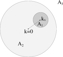
The following splitting of the integration area turns out to be convenient (cf. Figure 1):
A 1 := assign subscript 𝐴 1 absent \displaystyle A_{1}:= { 𝒌 ∈ ℝ 3 : k ~ = | 𝒌 − 𝒌 s | < k s 2 } , A 2 := { 𝒌 ∈ ℝ 3 : k < 2 k s ∧ | 𝒌 − 𝒌 s | ≥ k s 2 } , assign conditional-set 𝒌 superscript ℝ 3 ~ 𝑘 𝒌 subscript 𝒌 s subscript 𝑘 s 2 subscript 𝐴 2
conditional-set 𝒌 superscript ℝ 3 𝑘 2 subscript 𝑘 s 𝒌 subscript 𝒌 s subscript 𝑘 s 2 \displaystyle\{\boldsymbol{k}\in\mathbb{R}^{3}:\widetilde{k}=|\boldsymbol{k}-\boldsymbol{k}_{\text{s}}|<\frac{k_{\text{s}}}{2}\},\;A_{2}:=\{\boldsymbol{k}\in\mathbb{R}^{3}:k<2k_{\text{s}}\wedge|\boldsymbol{k}-\boldsymbol{k}_{\text{s}}|\geq\frac{k_{\text{s}}}{2}\},
A 3 := assign subscript 𝐴 3 absent \displaystyle A_{3}:= { 𝒌 ∈ ℝ 3 : k ≥ 3 2 k s } . conditional-set 𝒌 superscript ℝ 3 𝑘 3 2 subscript 𝑘 s \displaystyle\{\boldsymbol{k}\in\mathbb{R}^{3}:k\geq\frac{3}{2}k_{\text{s}}\}. (62)
Figure 1: Sketch of the three integration areas in the 𝒌 𝒌 \boldsymbol{k}
The areas A 2 subscript 𝐴 2 A_{2} A 3 subscript 𝐴 3 A_{3} A 1 subscript 𝐴 1 A_{1} A 2 subscript 𝐴 2 A_{2} A 3 subscript 𝐴 3 A_{3} k . 𝑘 k. 𝒙 ≠ 0 . 𝒙 0 \boldsymbol{x}\neq 0. 𝒙 = 0 𝒙 0 \boldsymbol{x}=0 k 𝑘 k A 3 subscript 𝐴 3 A_{3} 4
We first divide the integration area into A 1 ∪ A 2 subscript 𝐴 1 subscript 𝐴 2 A_{1}\cup A_{2} A 3 subscript 𝐴 3 A_{3} ρ ( 𝒌 ) : : 𝜌 𝒌 absent \rho(\boldsymbol{k}):
ρ ( 𝒌 ) = { 1 , for k < 3 2 k s , e exp ( − 1 1 − ( k − 3 2 k s ) 2 ( k s 2 ) 2 ) , for 3 2 k s ≤ k < 2 k s , 0 , for k ≥ 2 k s . 𝜌 𝒌 cases 1 for 𝑘
3 2 subscript 𝑘 s otherwise 𝑒 1 1 superscript 𝑘 3 2 subscript 𝑘 s 2 superscript subscript 𝑘 s 2 2 for 3 2 subscript 𝑘 s
𝑘 2 subscript 𝑘 s otherwise 0 for 𝑘
2 subscript 𝑘 s otherwise \rho(\boldsymbol{k})=\begin{cases}1,\text{ for }k<\frac{3}{2}k_{\text{s}},\\
e\exp\left(-\frac{1}{1-\frac{\left(k-\frac{3}{2}k_{\text{s}}\right)^{2}}{\left(\frac{k_{\text{s}}}{2}\right)^{2}}}\right),\text{ for }\frac{3}{2}k_{\text{s}}\leq k<2k_{\text{s}},\\
0,\text{ for }k\geq 2k_{\text{s}}.\end{cases} (63)
The mollifier has the following properties:
supp ρ = A 1 ∪ A 2 , | ρ ( 𝒌 ) | ≤ 1 , | 1 − ρ ( 𝒌 ) | ≤ 1 , formulae-sequence supp 𝜌 subscript 𝐴 1 subscript 𝐴 2 formulae-sequence 𝜌 𝒌 1 1 𝜌 𝒌 1 \displaystyle\operatorname{supp}\rho=A_{1}\cup A_{2},\;|\rho(\boldsymbol{k})|\leq 1,\;|1-\rho(\boldsymbol{k})|\leq 1,
There is an M > 0 such that: | ∂ k ρ ( 𝒌 ) | , | ∂ 𝒌 α ρ ( 𝒌 ) | ≤ M k s , | α | = 1 , formulae-sequence There is an 𝑀 0 such that: subscript 𝑘 𝜌 𝒌 formulae-sequence superscript subscript 𝒌 𝛼 𝜌 𝒌 𝑀 subscript 𝑘 s 𝛼 1 \displaystyle\text{There is an }M>0\text{ such that: }|\partial_{k}\rho(\boldsymbol{k})|,|\partial_{\boldsymbol{k}}^{\alpha}\rho(\boldsymbol{k})|\leq\frac{M}{k_{\text{s}}},\;|\alpha|=1,
and | ∂ k 2 ρ ( 𝒌 ) | , | ∂ 𝒌 α ρ ( 𝒌 ) | ≤ M k s 2 , | α | = 2 . formulae-sequence and superscript subscript 𝑘 2 𝜌 𝒌 superscript subscript 𝒌 𝛼 𝜌 𝒌
𝑀 superscript subscript 𝑘 s 2 𝛼 2 \displaystyle\text{and }|\partial_{k}^{2}\rho(\boldsymbol{k})|,|\partial_{\boldsymbol{k}}^{\alpha}\rho(\boldsymbol{k})|\leq\frac{M}{k_{\text{s}}^{2}},\;|\alpha|=2. (64)
Using ρ 𝜌 \rho 61
∫ e − i k 2 2 t + i 𝒌 ⋅ 𝒙 ( χ ( 𝒌 ) − χ ( 𝒌 s ) ) d 3 k = superscript 𝑒 𝑖 superscript 𝑘 2 2 𝑡 ⋅ 𝑖 𝒌 𝒙 𝜒 𝒌 𝜒 subscript 𝒌 s superscript 𝑑 3 𝑘 absent \displaystyle\int e^{-i\frac{k^{2}}{2}t+i\boldsymbol{k}\cdot\boldsymbol{x}}\left(\chi(\boldsymbol{k})-\chi(\boldsymbol{k}_{\text{s}})\right)d^{3}k= ∫ e − i k 2 2 t + i 𝒌 ⋅ 𝒙 ρ ( 𝒌 ) ( χ ( 𝒌 ) − χ ( 𝒌 s ) ) d 3 k superscript 𝑒 𝑖 superscript 𝑘 2 2 𝑡 ⋅ 𝑖 𝒌 𝒙 𝜌 𝒌 𝜒 𝒌 𝜒 subscript 𝒌 s superscript 𝑑 3 𝑘 \displaystyle\int e^{-i\frac{k^{2}}{2}t+i\boldsymbol{k}\cdot\boldsymbol{x}}\rho(\boldsymbol{k})\left(\chi(\boldsymbol{k})-\chi(\boldsymbol{k}_{\text{s}})\right)d^{3}k
+ ∫ e − i k 2 2 t + i 𝒌 ⋅ 𝒙 ( 1 − ρ ( 𝒌 ) ) ( χ ( 𝒌 ) − χ ( 𝒌 s ) ) d 3 k superscript 𝑒 𝑖 superscript 𝑘 2 2 𝑡 ⋅ 𝑖 𝒌 𝒙 1 𝜌 𝒌 𝜒 𝒌 𝜒 subscript 𝒌 s superscript 𝑑 3 𝑘 \displaystyle+\int e^{-i\frac{k^{2}}{2}t+i\boldsymbol{k}\cdot\boldsymbol{x}}\left(1-\rho(\boldsymbol{k})\right)\left(\chi(\boldsymbol{k})-\chi(\boldsymbol{k}_{\text{s}})\right)d^{3}k
= : absent : \displaystyle=: I 12 + I 3 . subscript 𝐼 12 subscript 𝐼 3 \displaystyle I_{12}+I_{3}. (65)
We start with the estimation of I 12 . subscript 𝐼 12 I_{12}.
f ( 𝒌 ) 𝑓 𝒌 \displaystyle f(\boldsymbol{k}) := ρ ( 𝒌 ) ( χ ( 𝒌 ) − χ ( 𝒌 s ) ) , 𝒌 ~ := 𝒌 − 𝒌 s formulae-sequence assign absent 𝜌 𝒌 𝜒 𝒌 𝜒 subscript 𝒌 s assign bold-~ 𝒌 𝒌 subscript 𝒌 s \displaystyle:=\rho(\boldsymbol{k})\left(\chi(\boldsymbol{k})-\chi(\boldsymbol{k}_{\text{s}})\right),\;\boldsymbol{\widetilde{k}}:=\boldsymbol{k}-\boldsymbol{k}_{\text{s}} (66)
and get with two partial integration w.r.t. to 𝒌 : : 𝒌 absent \boldsymbol{k}:
| I 12 | = subscript 𝐼 12 absent \displaystyle\left|I_{12}\right|= | ∫ e − i t ( k 2 2 − 𝒌 ⋅ 𝒌 s ) f ( 𝒌 ) d 3 k | superscript 𝑒 𝑖 𝑡 superscript 𝑘 2 2 ⋅ 𝒌 subscript 𝒌 s 𝑓 𝒌 superscript 𝑑 3 𝑘 \displaystyle\left|\int e^{-it\left(\frac{k^{2}}{2}-\boldsymbol{k}\cdot\boldsymbol{k}_{\text{s}}\right)}f(\boldsymbol{k})d^{3}k\right|
= \displaystyle= 1 t | ∫ ( ∇ 𝒌 e − i k 2 2 t + i 𝒌 ⋅ 𝒙 ) ⋅ 𝒌 ~ k ~ 2 f ( 𝒌 ) d 3 k | 1 𝑡 ⋅ subscript ∇ 𝒌 superscript 𝑒 𝑖 superscript 𝑘 2 2 𝑡 ⋅ 𝑖 𝒌 𝒙 bold-~ 𝒌 superscript ~ 𝑘 2 𝑓 𝒌 superscript 𝑑 3 𝑘 \displaystyle\frac{1}{t}\left|\int\left(\nabla_{\boldsymbol{k}}e^{-i\frac{k^{2}}{2}t+i\boldsymbol{k}\cdot\boldsymbol{x}}\right)\cdot\frac{\boldsymbol{\widetilde{k}}}{\widetilde{k}^{2}}f(\boldsymbol{k})d^{3}k\right|
= \displaystyle= 1 t | ∫ e − i k 2 2 t + i 𝒌 ⋅ 𝒙 ( 𝒌 ~ ⋅ ∇ 𝒌 f ( 𝒌 ) − f ( 𝒌 ) k ~ 2 ) d 3 k | 1 𝑡 superscript 𝑒 𝑖 superscript 𝑘 2 2 𝑡 ⋅ 𝑖 𝒌 𝒙 ⋅ bold-~ 𝒌 subscript ∇ 𝒌 𝑓 𝒌 𝑓 𝒌 superscript ~ 𝑘 2 superscript 𝑑 3 𝑘 \displaystyle\frac{1}{t}\left|\int e^{-i\frac{k^{2}}{2}t+i\boldsymbol{k}\cdot\boldsymbol{x}}\left(\frac{\boldsymbol{\widetilde{k}}\cdot\nabla_{\boldsymbol{k}}f(\boldsymbol{k})-f(\boldsymbol{k})}{\widetilde{k}^{2}}\right)d^{3}k\right|
= \displaystyle= 1 t 2 | ∫ ( ∇ 𝒌 e − i k 2 2 t + i 𝒌 ⋅ 𝒙 ) ⋅ 𝒌 ~ k ~ 2 ( 𝒌 ~ ⋅ ∇ 𝒌 f ( 𝒌 ) − f ( 𝒌 ) k ~ 2 ) d 3 k | 1 superscript 𝑡 2 ⋅ subscript ∇ 𝒌 superscript 𝑒 𝑖 superscript 𝑘 2 2 𝑡 ⋅ 𝑖 𝒌 𝒙 bold-~ 𝒌 superscript ~ 𝑘 2 ⋅ bold-~ 𝒌 subscript ∇ 𝒌 𝑓 𝒌 𝑓 𝒌 superscript ~ 𝑘 2 superscript 𝑑 3 𝑘 \displaystyle\frac{1}{t^{2}}\left|\int\left(\nabla_{\boldsymbol{k}}e^{-i\frac{k^{2}}{2}t+i\boldsymbol{k}\cdot\boldsymbol{x}}\right)\cdot\frac{\boldsymbol{\widetilde{k}}}{\widetilde{k}^{2}}\left(\frac{\boldsymbol{\widetilde{k}}\cdot\nabla_{\boldsymbol{k}}f(\boldsymbol{k})-f(\boldsymbol{k})}{\widetilde{k}^{2}}\right)d^{3}k\right|
= \displaystyle= 1 t 2 | ∫ e − i k 2 2 t + i 𝒌 ⋅ 𝒙 ( f ( 𝒌 ) − 𝒌 ~ ⋅ ∇ 𝒌 f ( 𝒌 ) k ~ 4 + 1 k ~ 4 ∑ | α 1 | + | α 2 | = 2 𝒌 ~ α 1 𝒌 ~ α 2 ∂ 𝒌 α 1 ∂ 𝒌 α 2 f ( 𝒌 ) ) d 3 k | 1 superscript 𝑡 2 superscript 𝑒 𝑖 superscript 𝑘 2 2 𝑡 ⋅ 𝑖 𝒌 𝒙 𝑓 𝒌 ⋅ bold-~ 𝒌 subscript ∇ 𝒌 𝑓 𝒌 superscript ~ 𝑘 4 1 superscript ~ 𝑘 4 subscript subscript 𝛼 1 subscript 𝛼 2 2 superscript bold-~ 𝒌 subscript 𝛼 1 superscript bold-~ 𝒌 subscript 𝛼 2 superscript subscript 𝒌 subscript 𝛼 1 superscript subscript 𝒌 subscript 𝛼 2 𝑓 𝒌 superscript 𝑑 3 𝑘 \displaystyle\frac{1}{t^{2}}\left|\int e^{-i\frac{k^{2}}{2}t+i\boldsymbol{k}\cdot\boldsymbol{x}}\left(\frac{f(\boldsymbol{k})-\boldsymbol{\widetilde{k}}\cdot\nabla_{\boldsymbol{k}}f(\boldsymbol{k})}{\widetilde{k}^{4}}+\frac{1}{\widetilde{k}^{4}}\sum\limits_{|\alpha_{1}|+|\alpha_{2}|=2}\boldsymbol{\widetilde{k}}^{\alpha_{1}}\boldsymbol{\widetilde{k}}^{\alpha_{2}}\partial_{\boldsymbol{k}}^{\alpha_{1}}\partial_{\boldsymbol{k}}^{\alpha_{2}}f(\boldsymbol{k})\right)d^{3}k\right|
≤ \displaystyle\leq 1 t 2 ∫ | f ( 𝒌 ) − 𝒌 ~ ⋅ ∇ 𝒌 f ( 𝒌 ) k ~ 4 | d 3 k + 1 t 2 ∫ | 1 k ~ 4 ∑ | α 1 | + | α 2 | = 2 𝒌 ~ α 1 𝒌 ~ α 2 ∂ 𝒌 α 1 ∂ 𝒌 α 2 f ( 𝒌 ) | d 3 k . 1 superscript 𝑡 2 𝑓 𝒌 ⋅ bold-~ 𝒌 subscript ∇ 𝒌 𝑓 𝒌 superscript ~ 𝑘 4 superscript 𝑑 3 𝑘 1 superscript 𝑡 2 1 superscript ~ 𝑘 4 subscript subscript 𝛼 1 subscript 𝛼 2 2 superscript bold-~ 𝒌 subscript 𝛼 1 superscript bold-~ 𝒌 subscript 𝛼 2 superscript subscript 𝒌 subscript 𝛼 1 superscript subscript 𝒌 subscript 𝛼 2 𝑓 𝒌 superscript 𝑑 3 𝑘 \displaystyle\frac{1}{t^{2}}\int\left|\frac{f(\boldsymbol{k})-\boldsymbol{\widetilde{k}}\cdot\nabla_{\boldsymbol{k}}f(\boldsymbol{k})}{\widetilde{k}^{4}}\right|d^{3}k+\frac{1}{t^{2}}\int\left|\frac{1}{\widetilde{k}^{4}}\sum\limits_{|\alpha_{1}|+|\alpha_{2}|=2}\boldsymbol{\widetilde{k}}^{\alpha_{1}}\boldsymbol{\widetilde{k}}^{\alpha_{2}}\partial_{\boldsymbol{k}}^{\alpha_{1}}\partial_{\boldsymbol{k}}^{\alpha_{2}}f(\boldsymbol{k})\right|d^{3}k. (67)
Because of the definition of ρ , 𝜌 \rho, 4 A 1 ∪ A 2 subscript 𝐴 1 subscript 𝐴 2 A_{1}\cup A_{2} 4 63 A 1 subscript 𝐴 1 A_{1} A 2 . subscript 𝐴 2 A_{2}. I 12 subscript 𝐼 12 I_{12}
| I 12 | ≤ subscript 𝐼 12 absent \displaystyle\left|I_{12}\right|\leq 1 t 2 ∫ A 1 | f ( 𝒌 ) − 𝒌 ~ ⋅ ∇ 𝒌 f ( 𝒌 ) k ~ 4 | d 3 k + 1 t 2 ∫ A 1 | 1 k ~ 4 ∑ | α 1 | + | α 2 | = 2 𝒌 ~ α 1 𝒌 ~ α 2 ∂ 𝒌 α 1 ∂ 𝒌 α 2 f ( 𝒌 ) | d 3 k 1 superscript 𝑡 2 subscript subscript 𝐴 1 𝑓 𝒌 ⋅ bold-~ 𝒌 subscript ∇ 𝒌 𝑓 𝒌 superscript ~ 𝑘 4 superscript 𝑑 3 𝑘 1 superscript 𝑡 2 subscript subscript 𝐴 1 1 superscript ~ 𝑘 4 subscript subscript 𝛼 1 subscript 𝛼 2 2 superscript bold-~ 𝒌 subscript 𝛼 1 superscript bold-~ 𝒌 subscript 𝛼 2 superscript subscript 𝒌 subscript 𝛼 1 superscript subscript 𝒌 subscript 𝛼 2 𝑓 𝒌 superscript 𝑑 3 𝑘 \displaystyle\frac{1}{t^{2}}\int\limits_{A_{1}}\left|\frac{f(\boldsymbol{k})-\boldsymbol{\widetilde{k}}\cdot\nabla_{\boldsymbol{k}}f(\boldsymbol{k})}{\widetilde{k}^{4}}\right|d^{3}k+\frac{1}{t^{2}}\int\limits_{A_{1}}\left|\frac{1}{\widetilde{k}^{4}}\sum\limits_{|\alpha_{1}|+|\alpha_{2}|=2}\boldsymbol{\widetilde{k}}^{\alpha_{1}}\boldsymbol{\widetilde{k}}^{\alpha_{2}}\partial_{\boldsymbol{k}}^{\alpha_{1}}\partial_{\boldsymbol{k}}^{\alpha_{2}}f(\boldsymbol{k})\right|d^{3}k
+ 1 t 2 ∫ A 2 | f ( 𝒌 ) − 𝒌 ~ ⋅ ∇ 𝒌 f ( 𝒌 ) k ~ 4 | d 3 k + 1 t 2 ∫ A 2 | 1 k ~ 4 ∑ | α 1 | + | α 2 | = 2 𝒌 ~ α 1 𝒌 ~ α 2 ∂ 𝒌 α 1 ∂ 𝒌 α 2 f ( 𝒌 ) | d 3 k 1 superscript 𝑡 2 subscript subscript 𝐴 2 𝑓 𝒌 ⋅ bold-~ 𝒌 subscript ∇ 𝒌 𝑓 𝒌 superscript ~ 𝑘 4 superscript 𝑑 3 𝑘 1 superscript 𝑡 2 subscript subscript 𝐴 2 1 superscript ~ 𝑘 4 subscript subscript 𝛼 1 subscript 𝛼 2 2 superscript bold-~ 𝒌 subscript 𝛼 1 superscript bold-~ 𝒌 subscript 𝛼 2 superscript subscript 𝒌 subscript 𝛼 1 superscript subscript 𝒌 subscript 𝛼 2 𝑓 𝒌 superscript 𝑑 3 𝑘 \displaystyle+\frac{1}{t^{2}}\int\limits_{A_{2}}\left|\frac{f(\boldsymbol{k})-\boldsymbol{\widetilde{k}}\cdot\nabla_{\boldsymbol{k}}f(\boldsymbol{k})}{\widetilde{k}^{4}}\right|d^{3}k+\frac{1}{t^{2}}\int\limits_{A_{2}}\left|\frac{1}{\widetilde{k}^{4}}\sum\limits_{|\alpha_{1}|+|\alpha_{2}|=2}\boldsymbol{\widetilde{k}}^{\alpha_{1}}\boldsymbol{\widetilde{k}}^{\alpha_{2}}\partial_{\boldsymbol{k}}^{\alpha_{1}}\partial_{\boldsymbol{k}}^{\alpha_{2}}f(\boldsymbol{k})\right|d^{3}k
= : absent : \displaystyle=: I 1 + 1 t 2 ∫ A 2 | f ( 𝒌 ) − 𝒌 ~ ⋅ ∇ 𝒌 f ( 𝒌 ) k ~ 4 | d 3 k + 1 t 2 ∫ A 2 | 1 k ~ 4 ∑ | α 1 | + | α 2 | = 2 𝒌 ~ α 1 𝒌 ~ α 2 ∂ 𝒌 α 1 ∂ 𝒌 α 2 f ( 𝒌 ) | d 3 k subscript 𝐼 1 1 superscript 𝑡 2 subscript subscript 𝐴 2 𝑓 𝒌 ⋅ bold-~ 𝒌 subscript ∇ 𝒌 𝑓 𝒌 superscript ~ 𝑘 4 superscript 𝑑 3 𝑘 1 superscript 𝑡 2 subscript subscript 𝐴 2 1 superscript ~ 𝑘 4 subscript subscript 𝛼 1 subscript 𝛼 2 2 superscript bold-~ 𝒌 subscript 𝛼 1 superscript bold-~ 𝒌 subscript 𝛼 2 superscript subscript 𝒌 subscript 𝛼 1 superscript subscript 𝒌 subscript 𝛼 2 𝑓 𝒌 superscript 𝑑 3 𝑘 \displaystyle I_{1}+\frac{1}{t^{2}}\int\limits_{A_{2}}\left|\frac{f(\boldsymbol{k})-\boldsymbol{\widetilde{k}}\cdot\nabla_{\boldsymbol{k}}f(\boldsymbol{k})}{\widetilde{k}^{4}}\right|d^{3}k+\frac{1}{t^{2}}\int\limits_{A_{2}}\left|\frac{1}{\widetilde{k}^{4}}\sum\limits_{|\alpha_{1}|+|\alpha_{2}|=2}\boldsymbol{\widetilde{k}}^{\alpha_{1}}\boldsymbol{\widetilde{k}}^{\alpha_{2}}\partial_{\boldsymbol{k}}^{\alpha_{1}}\partial_{\boldsymbol{k}}^{\alpha_{2}}f(\boldsymbol{k})\right|d^{3}k
= : absent : \displaystyle=: I 1 + I 2 . subscript 𝐼 1 subscript 𝐼 2 \displaystyle I_{1}+I_{2}. (68)
We estimate I 1 subscript 𝐼 1 I_{1} 4 63 𝒌 ∈ A 1 𝒌 subscript 𝐴 1 \boldsymbol{k}\in A_{1} ρ ( 𝒌 ) ≡ 1 𝜌 𝒌 1 \rho(\boldsymbol{k})\equiv 1 66 f ( 𝒌 ) = χ ( 𝒌 ) − χ ( 𝒌 s ) . 𝑓 𝒌 𝜒 𝒌 𝜒 subscript 𝒌 s f(\boldsymbol{k})=\chi(\boldsymbol{k})-\chi(\boldsymbol{k}_{\text{s}}). 𝒌 𝒌 \boldsymbol{k} 𝒌 ~ bold-~ 𝒌 \boldsymbol{\widetilde{k}} 66 I 1 1 superscript subscript 𝐼 1 1 I_{1}^{1} I 1 : : subscript 𝐼 1 absent I_{1}:
I 1 1 = superscript subscript 𝐼 1 1 absent \displaystyle I_{1}^{1}= 1 t 2 ∫ A 1 | f ( 𝒌 ) − 𝒌 ~ ⋅ ∇ 𝒌 f ( 𝒌 ) k ~ 4 | d 3 k 1 superscript 𝑡 2 subscript subscript 𝐴 1 𝑓 𝒌 ⋅ bold-~ 𝒌 subscript ∇ 𝒌 𝑓 𝒌 superscript ~ 𝑘 4 superscript 𝑑 3 𝑘 \displaystyle\frac{1}{t^{2}}\int\limits_{A_{1}}\left|\frac{f(\boldsymbol{k})-\boldsymbol{\widetilde{k}}\cdot\nabla_{\boldsymbol{k}}f(\boldsymbol{k})}{\widetilde{k}^{4}}\right|d^{3}k
= \displaystyle= 1 t 2 ∫ A 1 | χ ( 𝒌 ) − χ ( 𝒌 s ) − ( 𝒌 − 𝒌 s ) ⋅ ∇ 𝒌 χ ( 𝒌 ) ( 𝒌 − 𝒌 s ) 4 | d 3 k 1 superscript 𝑡 2 subscript subscript 𝐴 1 𝜒 𝒌 𝜒 subscript 𝒌 s ⋅ 𝒌 subscript 𝒌 s subscript ∇ 𝒌 𝜒 𝒌 superscript 𝒌 subscript 𝒌 s 4 superscript 𝑑 3 𝑘 \displaystyle\frac{1}{t^{2}}\int\limits_{A_{1}}\left|\frac{\chi(\boldsymbol{k})-\chi(\boldsymbol{k}_{\text{s}})-(\boldsymbol{k}-\boldsymbol{k}_{\text{s}})\cdot\nabla_{\boldsymbol{k}}\chi(\boldsymbol{k})}{(\boldsymbol{k}-\boldsymbol{k}_{\text{s}})^{4}}\right|d^{3}k
= \displaystyle= 1 t 2 ∫ A 1 | ∑ | α 1 | + | α 2 | = 2 ( 𝒌 − 𝒌 s ) α 1 ( 𝒌 − 𝒌 s ) α 2 ∂ 𝒌 α 1 ∂ 𝒌 α 2 χ ( 𝝃 ) 2 ( 𝒌 − 𝒌 s ) 4 | d 3 k 1 superscript 𝑡 2 subscript subscript 𝐴 1 subscript subscript 𝛼 1 subscript 𝛼 2 2 superscript 𝒌 subscript 𝒌 s subscript 𝛼 1 superscript 𝒌 subscript 𝒌 s subscript 𝛼 2 superscript subscript 𝒌 subscript 𝛼 1 superscript subscript 𝒌 subscript 𝛼 2 𝜒 𝝃 2 superscript 𝒌 subscript 𝒌 s 4 superscript 𝑑 3 𝑘 \displaystyle\frac{1}{t^{2}}\int\limits_{A_{1}}\left|\frac{\sum\limits_{|\alpha_{1}|+|\alpha_{2}|=2}(\boldsymbol{k}-\boldsymbol{k}_{\text{s}})^{\alpha_{1}}(\boldsymbol{k}-\boldsymbol{k}_{\text{s}})^{\alpha_{2}}\partial_{\boldsymbol{k}}^{\alpha_{1}}\partial_{\boldsymbol{k}}^{\alpha_{2}}\chi(\boldsymbol{\xi})}{2(\boldsymbol{k}-\boldsymbol{k}_{\text{s}})^{4}}\right|d^{3}k
= \displaystyle= 1 t 2 ∫ A 1 | ∑ | α 1 | + | α 2 | = 2 𝒌 ~ α 1 𝒌 ~ α 1 ∂ 𝒌 α 1 ∂ 𝒌 α 2 χ ( 𝝃 ) 2 k ~ 4 | d 3 k ~ , 1 superscript 𝑡 2 subscript subscript 𝐴 1 subscript subscript 𝛼 1 subscript 𝛼 2 2 superscript bold-~ 𝒌 subscript 𝛼 1 superscript bold-~ 𝒌 subscript 𝛼 1 superscript subscript 𝒌 subscript 𝛼 1 superscript subscript 𝒌 subscript 𝛼 2 𝜒 𝝃 2 superscript ~ 𝑘 4 superscript 𝑑 3 ~ 𝑘 \displaystyle\frac{1}{t^{2}}\int\limits_{A_{1}}\left|\frac{\sum\limits_{|\alpha_{1}|+|\alpha_{2}|=2}\boldsymbol{\widetilde{k}}^{\alpha_{1}}\boldsymbol{\widetilde{k}}^{\alpha_{1}}\partial_{\boldsymbol{k}}^{\alpha_{1}}\partial_{\boldsymbol{k}}^{\alpha_{2}}\chi(\boldsymbol{\xi})}{2\widetilde{k}^{4}}\right|d^{3}\widetilde{k}, (69)
where 𝝃 𝝃 \boldsymbol{\xi} 𝒌 s subscript 𝒌 s \boldsymbol{k}_{\text{s}} 𝒌 𝒌 \boldsymbol{k} ξ > k s 2 . 𝜉 subscript 𝑘 s 2 \xi>\frac{k_{\text{s}}}{2}. 4 ∂ k i ∂ k j χ ( 𝒌 ) ≤ C k − 1 , subscript subscript 𝑘 𝑖 subscript subscript 𝑘 𝑗 𝜒 𝒌 𝐶 superscript 𝑘 1 \partial_{k_{i}}\partial_{k_{j}}\chi(\boldsymbol{k})\leq Ck^{-1}, 4
I 1 1 ≤ superscript subscript 𝐼 1 1 absent \displaystyle I_{1}^{1}\leq 9 C 2 t 2 ∫ A 1 1 k ~ 2 ξ d 3 k ~ < 36 π C k s t 2 ∫ A 1 𝑑 k ~ = 18 π C t 2 . 9 𝐶 2 superscript 𝑡 2 subscript subscript 𝐴 1 1 superscript ~ 𝑘 2 𝜉 superscript 𝑑 3 ~ 𝑘 36 𝜋 𝐶 subscript 𝑘 s superscript 𝑡 2 subscript subscript 𝐴 1 differential-d ~ 𝑘 18 𝜋 𝐶 superscript 𝑡 2 \displaystyle\frac{9C}{2t^{2}}\int\limits_{A_{1}}\frac{1}{\widetilde{k}^{2}\xi}d^{3}\widetilde{k}<\frac{36\pi C}{k_{\text{s}}t^{2}}\int\limits_{A_{1}}d\widetilde{k}=\frac{18\pi C}{t^{2}}. (70)
The second term of I 1 subscript 𝐼 1 I_{1} 𝝃 𝝃 \boldsymbol{\xi} 𝒌 = 𝒌 ~ + 𝒌 s 𝒌 bold-~ 𝒌 subscript 𝒌 s \boldsymbol{k}=\boldsymbol{\widetilde{k}}+\boldsymbol{k}_{\text{s}} k > k s 2 . 𝑘 subscript 𝑘 s 2 k>\frac{k_{\text{s}}}{2}. I 1 subscript 𝐼 1 I_{1} t − 2 superscript 𝑡 2 t^{-2} 𝒌 s . subscript 𝒌 s \boldsymbol{k}_{\text{s}}. I 2 subscript 𝐼 2 I_{2} ρ ( 𝒌 ) ≠ 1 𝜌 𝒌 1 \rho(\boldsymbol{k})\neq 1 A 2 subscript 𝐴 2 A_{2} d 3 k superscript 𝑑 3 𝑘 d^{3}k A 2 . subscript 𝐴 2 A_{2}. I 2 subscript 𝐼 2 I_{2} L k s 3 𝐿 superscript subscript 𝑘 s 3 \frac{L}{k_{\text{s}}^{3}} L k s 2 k 𝐿 superscript subscript 𝑘 s 2 𝑘 \frac{L}{k_{\text{s}}^{2}k} L > 0 𝐿 0 L>0 𝒌 s . subscript 𝒌 s \boldsymbol{k}_{\text{s}}.
| f ( 𝒌 ) − 𝒌 ~ ⋅ ∇ 𝒌 f ( 𝒌 ) k ~ 4 | ≤ 𝑓 𝒌 ⋅ bold-~ 𝒌 subscript ∇ 𝒌 𝑓 𝒌 superscript ~ 𝑘 4 absent \displaystyle\left|\frac{f(\boldsymbol{k})-\boldsymbol{\widetilde{k}}\cdot\nabla_{\boldsymbol{k}}f(\boldsymbol{k})}{\widetilde{k}^{4}}\right|\leq | ρ ( 𝒌 ) ( χ ( 𝒌 ) − χ ( 𝒌 s ) ) k ~ 4 | + | | ∇ 𝒌 f ( 𝒌 ) | k ~ 3 | 𝜌 𝒌 𝜒 𝒌 𝜒 subscript 𝒌 s superscript ~ 𝑘 4 subscript ∇ 𝒌 𝑓 𝒌 superscript ~ 𝑘 3 \displaystyle\left|\frac{\rho(\boldsymbol{k})(\chi(\boldsymbol{k})-\chi(\boldsymbol{k}_{\text{s}}))}{\widetilde{k}^{4}}\right|+\left|\frac{\left|\nabla_{\boldsymbol{k}}f(\boldsymbol{k})\right|}{\widetilde{k}^{3}}\right|
≤ \displaystyle\leq | χ ( 𝒌 ) − χ ( 𝒌 s ) k ~ 4 | + ∑ i = 1 3 | | ∂ k i χ ( 𝒌 ) | k ~ 3 | + ∑ i = 1 3 | | ( χ ( 𝒌 ) − χ ( 𝒌 s ) ) ∂ k i ρ ( 𝒌 ) | k ~ 3 | . 𝜒 𝒌 𝜒 subscript 𝒌 s superscript ~ 𝑘 4 superscript subscript 𝑖 1 3 subscript subscript 𝑘 𝑖 𝜒 𝒌 superscript ~ 𝑘 3 superscript subscript 𝑖 1 3 𝜒 𝒌 𝜒 subscript 𝒌 s subscript subscript 𝑘 𝑖 𝜌 𝒌 superscript ~ 𝑘 3 \displaystyle\left|\frac{\chi(\boldsymbol{k})-\chi(\boldsymbol{k}_{\text{s}})}{\widetilde{k}^{4}}\right|+\sum\limits_{i=1}^{3}\left|\frac{\left|\partial_{k_{i}}\chi(\boldsymbol{k})\right|}{\widetilde{k}^{3}}\right|+\sum\limits_{i=1}^{3}\left|\frac{\left|(\chi(\boldsymbol{k})-\chi(\boldsymbol{k}_{\text{s}}))\partial_{k_{i}}\rho(\boldsymbol{k})\right|}{\widetilde{k}^{3}}\right|. (71)
By mean value theorem there exists a 𝝃 ∈ ( 𝒌 s , 𝒌 ) 𝝃 subscript 𝒌 s 𝒌 \boldsymbol{\xi}\in(\boldsymbol{k}_{\text{s}},\boldsymbol{k})
| χ ( 𝒌 ) − χ ( 𝒌 s ) | = 𝜒 𝒌 𝜒 subscript 𝒌 s absent \displaystyle|\chi(\boldsymbol{k})-\chi(\boldsymbol{k}_{\text{s}})|= | ∇ 𝒌 χ ( 𝝃 ) | | 𝒌 − 𝒌 s | ≤ C k + C k s , subscript ∇ 𝒌 𝜒 𝝃 𝒌 subscript 𝒌 s 𝐶 𝑘 𝐶 subscript 𝑘 s \displaystyle\left|\nabla_{\boldsymbol{k}}\chi(\boldsymbol{\xi})\right||\boldsymbol{k}-\boldsymbol{k}_{\text{s}}|\leq Ck+Ck_{\text{s}}, (72)
since χ ( 𝒌 ) ∈ 𝒦 ^ 𝜒 𝒌 ^ 𝒦 \chi(\boldsymbol{k})\in\widehat{\mathcal{K}} 72 4 𝒌 ∈ A 2 𝒌 subscript 𝐴 2 \boldsymbol{k}\in A_{2} k < 2 k s 𝑘 2 subscript 𝑘 s k<2k_{\text{s}} k ~ ≥ k s 2 ~ 𝑘 subscript 𝑘 s 2 \widetilde{k}\geq\frac{k_{\text{s}}}{2} | ∂ k i χ ( 𝒌 ) | ≤ C , i = { 1 , 2 , 3 } formulae-sequence subscript subscript 𝑘 𝑖 𝜒 𝒌 𝐶 𝑖 1 2 3 \left|\partial_{k_{i}}\chi(\boldsymbol{k})\right|\leq C,\;i=\{1,2,3\}
| f ( 𝒌 ) − 𝒌 ~ ⋅ ∇ 𝒌 f ( 𝒌 ) k ~ 4 | ≤ 𝑓 𝒌 ⋅ bold-~ 𝒌 subscript ∇ 𝒌 𝑓 𝒌 superscript ~ 𝑘 4 absent \displaystyle\left|\frac{f(\boldsymbol{k})-\boldsymbol{\widetilde{k}}\cdot\nabla_{\boldsymbol{k}}f(\boldsymbol{k})}{\widetilde{k}^{4}}\right|\leq 32 C k s 3 + 16 C k s 3 + 24 C k s 3 + 48 C M k s 3 + 24 C M k s 3 . 32 𝐶 superscript subscript 𝑘 s 3 16 𝐶 superscript subscript 𝑘 s 3 24 𝐶 superscript subscript 𝑘 s 3 48 𝐶 𝑀 superscript subscript 𝑘 s 3 24 𝐶 𝑀 superscript subscript 𝑘 s 3 \displaystyle\frac{32C}{k_{\text{s}}^{3}}+\frac{16C}{k_{\text{s}}^{3}}+\frac{24C}{k_{\text{s}}^{3}}+\frac{48CM}{k_{\text{s}}^{3}}+\frac{24CM}{k_{\text{s}}^{3}}. (73)
Similarly we estimate the integrand of the second term of I 2 subscript 𝐼 2 I_{2} 4 | α 1 | + | α 2 | = 2 subscript 𝛼 1 subscript 𝛼 2 2 |\alpha_{1}|+|\alpha_{2}|=2
| 1 k ~ 4 𝒌 ~ α 1 𝒌 ~ α 1 ∂ 𝒌 α 1 ∂ 𝒌 α 2 f ( 𝒌 ) | ≤ 1 superscript ~ 𝑘 4 superscript bold-~ 𝒌 subscript 𝛼 1 superscript bold-~ 𝒌 subscript 𝛼 1 superscript subscript 𝒌 subscript 𝛼 1 superscript subscript 𝒌 subscript 𝛼 2 𝑓 𝒌 absent \displaystyle\left|\frac{1}{\widetilde{k}^{4}}\boldsymbol{\widetilde{k}}^{\alpha_{1}}\boldsymbol{\widetilde{k}}^{\alpha_{1}}\partial_{\boldsymbol{k}}^{\alpha_{1}}\partial_{\boldsymbol{k}}^{\alpha_{2}}f(\boldsymbol{k})\right|\leq | 1 k ~ 2 ∂ 𝒌 α 1 ∂ 𝒌 α 2 f ( 𝒌 ) | 1 superscript ~ 𝑘 2 superscript subscript 𝒌 subscript 𝛼 1 superscript subscript 𝒌 subscript 𝛼 2 𝑓 𝒌 \displaystyle\left|\frac{1}{\widetilde{k}^{2}}\partial_{\boldsymbol{k}}^{\alpha_{1}}\partial_{\boldsymbol{k}}^{\alpha_{2}}f(\boldsymbol{k})\right|
≤ \displaystyle\leq 4 | χ ( 𝒌 ) − χ ( 𝒌 s ) | | ∂ 𝒌 α 1 ∂ 𝒌 α 2 ρ ( 𝒌 ) | k s 2 + 4 | ∂ 𝒌 α 1 ρ ( 𝒌 ) | | ∂ 𝒌 α 2 χ ( 𝒌 ) | k s 2 4 𝜒 𝒌 𝜒 subscript 𝒌 s superscript subscript 𝒌 subscript 𝛼 1 superscript subscript 𝒌 subscript 𝛼 2 𝜌 𝒌 superscript subscript 𝑘 s 2 4 superscript subscript 𝒌 subscript 𝛼 1 𝜌 𝒌 superscript subscript 𝒌 subscript 𝛼 2 𝜒 𝒌 superscript subscript 𝑘 s 2 \displaystyle\frac{4\left|\chi(\boldsymbol{k})-\chi(\boldsymbol{k}_{\text{s}})\right|\left|\partial_{\boldsymbol{k}}^{\alpha_{1}}\partial_{\boldsymbol{k}}^{\alpha_{2}}\rho(\boldsymbol{k})\right|}{k_{\text{s}}^{2}}+\frac{4\left|\partial_{\boldsymbol{k}}^{\alpha_{1}}\rho(\boldsymbol{k})\right|\left|\partial_{\boldsymbol{k}}^{\alpha_{2}}\chi(\boldsymbol{k})\right|}{k_{\text{s}}^{2}}
+ 4 | ∂ 𝒌 α 2 ρ ( 𝒌 ) | | ∂ 𝒌 α 1 χ ( 𝒌 ) | k s 2 + 4 | ∂ 𝒌 α 1 ∂ 𝒌 α 2 χ ( 𝒌 ) | k s 2 4 superscript subscript 𝒌 subscript 𝛼 2 𝜌 𝒌 superscript subscript 𝒌 subscript 𝛼 1 𝜒 𝒌 superscript subscript 𝑘 s 2 4 superscript subscript 𝒌 subscript 𝛼 1 superscript subscript 𝒌 subscript 𝛼 2 𝜒 𝒌 superscript subscript 𝑘 s 2 \displaystyle+\frac{4\left|\partial_{\boldsymbol{k}}^{\alpha_{2}}\rho(\boldsymbol{k})\right|\left|\partial_{\boldsymbol{k}}^{\alpha_{1}}\chi(\boldsymbol{k})\right|}{k_{\text{s}}^{2}}+\frac{4\left|\partial_{\boldsymbol{k}}^{\alpha_{1}}\partial_{\boldsymbol{k}}^{\alpha_{2}}\chi(\boldsymbol{k})\right|}{k_{\text{s}}^{2}}
≤ \displaystyle\leq 8 C M k s 3 + 4 C M k s 3 + 8 C M k s 3 + 4 C k s 2 k . 8 𝐶 𝑀 superscript subscript 𝑘 s 3 4 𝐶 𝑀 superscript subscript 𝑘 s 3 8 𝐶 𝑀 superscript subscript 𝑘 s 3 4 𝐶 superscript subscript 𝑘 s 2 𝑘 \displaystyle\frac{8CM}{k_{\text{s}}^{3}}+\frac{4CM}{k_{\text{s}}^{3}}+\frac{8CM}{k_{\text{s}}^{3}}+\frac{4C}{k_{\text{s}}^{2}k}. (74)
It remains to estimate I 3 subscript 𝐼 3 I_{3} 4 ρ ϵ ( 𝒌 ) : : subscript 𝜌 italic-ϵ 𝒌 absent \rho_{\epsilon}(\boldsymbol{k}):
ρ ϵ ( 𝒌 ) = { 1 , for k < 1 ϵ , e − ( k − 1 ϵ ) 2 , for k ≥ 1 ϵ , subscript 𝜌 italic-ϵ 𝒌 cases 1 for 𝑘
1 italic-ϵ otherwise superscript 𝑒 superscript 𝑘 1 italic-ϵ 2 for 𝑘
1 italic-ϵ otherwise \rho_{\epsilon}(\boldsymbol{k})=\begin{cases}1,\text{ for }k<\frac{1}{\epsilon},\\
e^{-\left(k-\frac{1}{\epsilon}\right)^{2}},\text{ for }k\geq\frac{1}{\epsilon},\end{cases} (75)
with 0 < ϵ < min ( 1 2 k s ; 1 ) . 0 italic-ϵ 1 2 subscript 𝑘 s 1 0<\epsilon<\min(\frac{1}{2k_{\text{s}}};1). I 3 subscript 𝐼 3 I_{3} 4
I 3 = subscript 𝐼 3 absent \displaystyle I_{3}= ∫ e − i k 2 2 t + i 𝒌 ⋅ 𝒙 ( 1 − ρ ( 𝒌 ) ) ( χ ( 𝒌 ) − χ ( 𝒌 s ) ) d 3 k superscript 𝑒 𝑖 superscript 𝑘 2 2 𝑡 ⋅ 𝑖 𝒌 𝒙 1 𝜌 𝒌 𝜒 𝒌 𝜒 subscript 𝒌 s superscript 𝑑 3 𝑘 \displaystyle\int e^{-i\frac{k^{2}}{2}t+i\boldsymbol{k}\cdot\boldsymbol{x}}\left(1-\rho(\boldsymbol{k})\right)\left(\chi(\boldsymbol{k})-\chi(\boldsymbol{k}_{\text{s}})\right)d^{3}k
= \displaystyle= ∫ e − i k 2 2 t + i 𝒌 ⋅ 𝒙 ( 1 − ρ ( 𝒌 ) ) ( 1 − ρ ϵ ( 𝒌 ) + ρ ϵ ( 𝒌 ) ) ( χ ( 𝒌 ) − χ ( 𝒌 s ) ) d 3 k superscript 𝑒 𝑖 superscript 𝑘 2 2 𝑡 ⋅ 𝑖 𝒌 𝒙 1 𝜌 𝒌 1 subscript 𝜌 italic-ϵ 𝒌 subscript 𝜌 italic-ϵ 𝒌 𝜒 𝒌 𝜒 subscript 𝒌 s superscript 𝑑 3 𝑘 \displaystyle\int e^{-i\frac{k^{2}}{2}t+i\boldsymbol{k}\cdot\boldsymbol{x}}\left(1-\rho(\boldsymbol{k})\right)\left(1-\rho_{\epsilon}(\boldsymbol{k})+\rho_{\epsilon}(\boldsymbol{k})\right)\left(\chi(\boldsymbol{k})-\chi(\boldsymbol{k}_{\text{s}})\right)d^{3}k
= \displaystyle= lim ϵ → 0 ∫ e − i k 2 2 t + i 𝒌 ⋅ 𝒙 ( 1 − ρ ( 𝒌 ) ) ( 1 − ρ ϵ ( 𝒌 ) + ρ ϵ ( 𝒌 ) ) ( χ ( 𝒌 ) − χ ( 𝒌 s ) ) d 3 k subscript → italic-ϵ 0 superscript 𝑒 𝑖 superscript 𝑘 2 2 𝑡 ⋅ 𝑖 𝒌 𝒙 1 𝜌 𝒌 1 subscript 𝜌 italic-ϵ 𝒌 subscript 𝜌 italic-ϵ 𝒌 𝜒 𝒌 𝜒 subscript 𝒌 s superscript 𝑑 3 𝑘 \displaystyle\lim\limits_{\epsilon\to 0}\int e^{-i\frac{k^{2}}{2}t+i\boldsymbol{k}\cdot\boldsymbol{x}}\left(1-\rho(\boldsymbol{k})\right)\left(1-\rho_{\epsilon}(\boldsymbol{k})+\rho_{\epsilon}(\boldsymbol{k})\right)\left(\chi(\boldsymbol{k})-\chi(\boldsymbol{k}_{\text{s}})\right)d^{3}k
= \displaystyle= lim ϵ → 0 ∫ e − i k 2 2 t + i 𝒌 ⋅ 𝒙 ( 1 − ρ ( 𝒌 ) ) ρ ϵ ( 𝒌 ) ( χ ( 𝒌 ) − χ ( 𝒌 s ) ) d 3 k subscript → italic-ϵ 0 superscript 𝑒 𝑖 superscript 𝑘 2 2 𝑡 ⋅ 𝑖 𝒌 𝒙 1 𝜌 𝒌 subscript 𝜌 italic-ϵ 𝒌 𝜒 𝒌 𝜒 subscript 𝒌 s superscript 𝑑 3 𝑘 \displaystyle\lim\limits_{\epsilon\to 0}\int e^{-i\frac{k^{2}}{2}t+i\boldsymbol{k}\cdot\boldsymbol{x}}\left(1-\rho(\boldsymbol{k})\right)\rho_{\epsilon}(\boldsymbol{k})\left(\chi(\boldsymbol{k})-\chi(\boldsymbol{k}_{\text{s}})\right)d^{3}k
+ lim ϵ → 0 ∫ e − i k 2 2 t + i 𝒌 ⋅ 𝒙 ( 1 − ρ ( 𝒌 ) ) ( 1 − ρ ϵ ( 𝒌 ) ) ( χ ( 𝒌 ) − χ ( 𝒌 s ) ) d 3 k subscript → italic-ϵ 0 superscript 𝑒 𝑖 superscript 𝑘 2 2 𝑡 ⋅ 𝑖 𝒌 𝒙 1 𝜌 𝒌 1 subscript 𝜌 italic-ϵ 𝒌 𝜒 𝒌 𝜒 subscript 𝒌 s superscript 𝑑 3 𝑘 \displaystyle+\lim\limits_{\epsilon\to 0}\int e^{-i\frac{k^{2}}{2}t+i\boldsymbol{k}\cdot\boldsymbol{x}}\left(1-\rho(\boldsymbol{k})\right)\left(1-\rho_{\epsilon}(\boldsymbol{k})\right)\left(\chi(\boldsymbol{k})-\chi(\boldsymbol{k}_{\text{s}})\right)d^{3}k
= \displaystyle= lim ϵ → 0 ∫ e − i k 2 2 t + i 𝒌 ⋅ 𝒙 ( 1 − ρ ( 𝒌 ) ) ρ ϵ ( 𝒌 ) ( χ ( 𝒌 ) − χ ( 𝒌 s ) ) d 3 k subscript → italic-ϵ 0 superscript 𝑒 𝑖 superscript 𝑘 2 2 𝑡 ⋅ 𝑖 𝒌 𝒙 1 𝜌 𝒌 subscript 𝜌 italic-ϵ 𝒌 𝜒 𝒌 𝜒 subscript 𝒌 s superscript 𝑑 3 𝑘 \displaystyle\lim\limits_{\epsilon\to 0}\int e^{-i\frac{k^{2}}{2}t+i\boldsymbol{k}\cdot\boldsymbol{x}}\left(1-\rho(\boldsymbol{k})\right)\rho_{\epsilon}(\boldsymbol{k})\left(\chi(\boldsymbol{k})-\chi(\boldsymbol{k}_{\text{s}})\right)d^{3}k
+ lim ϵ → 0 ∫ k = 1 ϵ ∞ e − i k 2 2 t + i 𝒌 ⋅ 𝒙 ( 1 − ρ ϵ ( 𝒌 ) ) ( χ ( 𝒌 ) − χ ( 𝒌 s ) ) d 3 k , subscript → italic-ϵ 0 superscript subscript 𝑘 1 italic-ϵ superscript 𝑒 𝑖 superscript 𝑘 2 2 𝑡 ⋅ 𝑖 𝒌 𝒙 1 subscript 𝜌 italic-ϵ 𝒌 𝜒 𝒌 𝜒 subscript 𝒌 s superscript 𝑑 3 𝑘 \displaystyle+\lim\limits_{\epsilon\to 0}\int\limits_{k=\frac{1}{\epsilon}}^{\infty}e^{-i\frac{k^{2}}{2}t+i\boldsymbol{k}\cdot\boldsymbol{x}}\left(1-\rho_{\epsilon}(\boldsymbol{k})\right)\left(\chi(\boldsymbol{k})-\chi(\boldsymbol{k}_{\text{s}})\right)d^{3}k, (76)
since 1 − ρ ≡ 1 1 𝜌 1 1-\rho\equiv 1 supp ( 1 − ρ ϵ ) supp 1 subscript 𝜌 italic-ϵ \operatorname{supp}(1-\rho_{\epsilon}) 63 75 4 χ ( 𝒌 ) ∈ 𝒦 ^ 𝜒 𝒌 ^ 𝒦 \chi(\boldsymbol{k})\in\widehat{\mathcal{K}} I 3 subscript 𝐼 3 I_{3}
I 3 = subscript 𝐼 3 absent \displaystyle I_{3}= lim ϵ → 0 ∫ e − i t ( k 2 2 − 𝒌 ⋅ 𝒌 s ) ( 1 − ρ ( 𝒌 ) ) ρ ϵ ( 𝒌 ) ( χ ( 𝒌 ) − χ ( 𝒌 s ) ) d 3 k subscript → italic-ϵ 0 superscript 𝑒 𝑖 𝑡 superscript 𝑘 2 2 ⋅ 𝒌 subscript 𝒌 s 1 𝜌 𝒌 subscript 𝜌 italic-ϵ 𝒌 𝜒 𝒌 𝜒 subscript 𝒌 s superscript 𝑑 3 𝑘 \displaystyle\lim\limits_{\epsilon\to 0}\int e^{-it\left(\frac{k^{2}}{2}-\boldsymbol{k}\cdot\boldsymbol{k}_{\text{s}}\right)}\left(1-\rho(\boldsymbol{k})\right)\rho_{\epsilon}(\boldsymbol{k})\left(\chi(\boldsymbol{k})-\chi(\boldsymbol{k}_{\text{s}})\right)d^{3}k
= : absent : \displaystyle=: lim ϵ → 0 ∫ e − i t ( k 2 2 − 𝒌 ⋅ 𝒌 s ) f ϵ ( 𝒌 , 𝒌 s ) k 2 𝑑 k 𝑑 Ω . subscript → italic-ϵ 0 superscript 𝑒 𝑖 𝑡 superscript 𝑘 2 2 ⋅ 𝒌 subscript 𝒌 s subscript 𝑓 italic-ϵ 𝒌 subscript 𝒌 s superscript 𝑘 2 differential-d 𝑘 differential-d Ω \displaystyle\lim\limits_{\epsilon\to 0}\int e^{-it\left(\frac{k^{2}}{2}-\boldsymbol{k}\cdot\boldsymbol{k}_{\text{s}}\right)}f_{\epsilon}(\boldsymbol{k},\boldsymbol{k}_{\text{s}})k^{2}dkd\Omega. (77)
We will perform now two partial integrations w.r.t. k 𝑘 k
| I 3 | = subscript 𝐼 3 absent \displaystyle|I_{3}|= | lim ϵ → 0 1 t ∫ e − i t ( k 2 2 − 𝒌 ⋅ 𝒌 s ) ∂ k ( k 2 f ϵ ( 𝒌 , 𝒌 s ) k − 𝒆 k ⋅ 𝒌 s ) d k d Ω | subscript → italic-ϵ 0 1 𝑡 superscript 𝑒 𝑖 𝑡 superscript 𝑘 2 2 ⋅ 𝒌 subscript 𝒌 s subscript 𝑘 superscript 𝑘 2 subscript 𝑓 italic-ϵ 𝒌 subscript 𝒌 s 𝑘 ⋅ subscript 𝒆 𝑘 subscript 𝒌 s 𝑑 𝑘 𝑑 Ω \displaystyle\left|\lim\limits_{\epsilon\to 0}\frac{1}{t}\int e^{-it\left(\frac{k^{2}}{2}-\boldsymbol{k}\cdot\boldsymbol{k}_{\text{s}}\right)}\partial_{k}\left(\frac{k^{2}f_{\epsilon}(\boldsymbol{k},\boldsymbol{k}_{\text{s}})}{k-\boldsymbol{e}_{k}\cdot\boldsymbol{k}_{\text{s}}}\right)dkd\Omega\right|
= \displaystyle= | lim ϵ → 0 1 t 2 ∫ e − i t ( k 2 2 − 𝒌 ⋅ 𝒌 s ) ∂ k ( 1 k − 𝒆 k ⋅ 𝒌 s ∂ k ( k 2 f ϵ ( 𝒌 , 𝒌 s ) k − 𝒆 k ⋅ 𝒌 s ) ) d k d Ω | subscript → italic-ϵ 0 1 superscript 𝑡 2 superscript 𝑒 𝑖 𝑡 superscript 𝑘 2 2 ⋅ 𝒌 subscript 𝒌 s subscript 𝑘 1 𝑘 ⋅ subscript 𝒆 𝑘 subscript 𝒌 s subscript 𝑘 superscript 𝑘 2 subscript 𝑓 italic-ϵ 𝒌 subscript 𝒌 s 𝑘 ⋅ subscript 𝒆 𝑘 subscript 𝒌 s 𝑑 𝑘 𝑑 Ω \displaystyle\left|\lim\limits_{\epsilon\to 0}\frac{1}{t^{2}}\int e^{-it\left(\frac{k^{2}}{2}-\boldsymbol{k}\cdot\boldsymbol{k}_{\text{s}}\right)}\partial_{k}\left(\frac{1}{k-\boldsymbol{e}_{k}\cdot\boldsymbol{k}_{\text{s}}}\partial_{k}\left(\frac{k^{2}f_{\epsilon}(\boldsymbol{k},\boldsymbol{k}_{\text{s}})}{k-\boldsymbol{e}_{k}\cdot\boldsymbol{k}_{\text{s}}}\right)\right)dkd\Omega\right|
≤ \displaystyle\leq 1 t 2 lim ϵ → 0 ∫ | ∂ k ( 1 k − 𝒆 k ⋅ 𝒌 s ∂ k ( k 2 f ϵ ( 𝒌 , 𝒌 s ) k − 𝒆 k ⋅ 𝒌 s ) ) | 𝑑 k 𝑑 Ω 1 superscript 𝑡 2 subscript → italic-ϵ 0 subscript 𝑘 1 𝑘 ⋅ subscript 𝒆 𝑘 subscript 𝒌 s subscript 𝑘 superscript 𝑘 2 subscript 𝑓 italic-ϵ 𝒌 subscript 𝒌 s 𝑘 ⋅ subscript 𝒆 𝑘 subscript 𝒌 s differential-d 𝑘 differential-d Ω \displaystyle\frac{1}{t^{2}}\lim\limits_{\epsilon\to 0}\int\left|\partial_{k}\left(\frac{1}{k-\boldsymbol{e}_{k}\cdot\boldsymbol{k}_{\text{s}}}\partial_{k}\left(\frac{k^{2}f_{\epsilon}(\boldsymbol{k},\boldsymbol{k}_{\text{s}})}{k-\boldsymbol{e}_{k}\cdot\boldsymbol{k}_{\text{s}}}\right)\right)\right|dkd\Omega
= : absent : \displaystyle=: 1 t 2 lim ϵ → 0 ∫ k ≥ 3 2 k s | D | 𝑑 k 𝑑 Ω 1 superscript 𝑡 2 subscript → italic-ϵ 0 subscript 𝑘 3 2 subscript 𝑘 s 𝐷 differential-d 𝑘 differential-d Ω \displaystyle\frac{1}{t^{2}}\lim\limits_{\epsilon\to 0}\int\limits_{k\geq\frac{3}{2}k_{\text{s}}}|D|dkd\Omega
≤ \displaystyle\leq 1 t 2 lim ϵ → 0 ∫ 3 2 k s ≤ k < 2 k s | D | 𝑑 k 𝑑 Ω + 1 t 2 lim ϵ → 0 ∫ 2 k s ≤ k < 1 ϵ | D | 𝑑 k 𝑑 Ω + 1 t 2 lim ϵ → 0 ∫ k ≥ 1 ϵ | D | 𝑑 k 𝑑 Ω 1 superscript 𝑡 2 subscript → italic-ϵ 0 subscript 3 2 subscript 𝑘 s 𝑘 2 subscript 𝑘 s 𝐷 differential-d 𝑘 differential-d Ω 1 superscript 𝑡 2 subscript → italic-ϵ 0 subscript 2 subscript 𝑘 s 𝑘 1 italic-ϵ 𝐷 differential-d 𝑘 differential-d Ω 1 superscript 𝑡 2 subscript → italic-ϵ 0 subscript 𝑘 1 italic-ϵ 𝐷 differential-d 𝑘 differential-d Ω \displaystyle\frac{1}{t^{2}}\lim\limits_{\epsilon\to 0}\int\limits_{\frac{3}{2}k_{\text{s}}\leq k<2k_{\text{s}}}|D|dkd\Omega+\frac{1}{t^{2}}\lim\limits_{\epsilon\to 0}\int\limits_{2k_{\text{s}}\leq k<\frac{1}{\epsilon}}|D|dkd\Omega+\frac{1}{t^{2}}\lim\limits_{\epsilon\to 0}\int\limits_{k\geq\frac{1}{\epsilon}}|D|dkd\Omega
= : absent : \displaystyle=: I 3 1 + I 3 2 + I 3 3 . superscript subscript 𝐼 3 1 superscript subscript 𝐼 3 2 superscript subscript 𝐼 3 3 \displaystyle I_{3}^{1}+I_{3}^{2}+I_{3}^{3}. (78)
We start with the estimation of I 3 1 . superscript subscript 𝐼 3 1 I_{3}^{1}. D 𝐷 D k s − 1 . superscript subscript 𝑘 s 1 k_{\text{s}}^{-1}. ρ ϵ ( 𝒌 ) ≡ 1 subscript 𝜌 italic-ϵ 𝒌 1 \rho_{\epsilon}(\boldsymbol{k})\equiv 1 D 𝐷 D ( ⋅ ) ′ superscript ⋅ ′ (\cdot)^{\prime} k 𝑘 k
| D | ≤ 𝐷 absent \displaystyle|D|\leq | k 2 ( k − 𝒆 𝒌 ⋅ 𝒌 s ) 2 | | ( ( 1 − ρ ( 𝒌 ) ) ( χ ( 𝒌 ) − χ ( 𝒌 s ) ) ) ′′ | superscript 𝑘 2 superscript 𝑘 ⋅ subscript 𝒆 𝒌 subscript 𝒌 s 2 superscript 1 𝜌 𝒌 𝜒 𝒌 𝜒 subscript 𝒌 s ′′ \displaystyle\left|\frac{k^{2}}{(k-\boldsymbol{e}_{\boldsymbol{k}}\cdot\boldsymbol{k}_{\text{s}})^{2}}\right|\left|\left((1-\rho(\boldsymbol{k}))(\chi(\boldsymbol{k})-\chi(\boldsymbol{k}_{\text{s}}))\right)^{\prime\prime}\right|
+ | ( k 2 ( k − 𝒆 𝒌 ⋅ 𝒌 s ) 2 ) ′ + 1 k − 𝒆 𝒌 ⋅ 𝒌 s ( k 2 k − 𝒆 𝒌 ⋅ 𝒌 s ) ′ | | ( ( 1 − ρ ( 𝒌 ) ) ( χ ( 𝒌 ) − χ ( 𝒌 s ) ) ) ′ | superscript superscript 𝑘 2 superscript 𝑘 ⋅ subscript 𝒆 𝒌 subscript 𝒌 s 2 ′ 1 𝑘 ⋅ subscript 𝒆 𝒌 subscript 𝒌 s superscript superscript 𝑘 2 𝑘 ⋅ subscript 𝒆 𝒌 subscript 𝒌 s ′ superscript 1 𝜌 𝒌 𝜒 𝒌 𝜒 subscript 𝒌 s ′ \displaystyle+\left|\left(\frac{k^{2}}{(k-\boldsymbol{e}_{\boldsymbol{k}}\cdot\boldsymbol{k}_{\text{s}})^{2}}\right)^{\prime}+\frac{1}{k-\boldsymbol{e}_{\boldsymbol{k}}\cdot\boldsymbol{k}_{\text{s}}}\left(\frac{k^{2}}{k-\boldsymbol{e}_{\boldsymbol{k}}\cdot\boldsymbol{k}_{\text{s}}}\right)^{\prime}\right|\left|\left((1-\rho(\boldsymbol{k}))(\chi(\boldsymbol{k})-\chi(\boldsymbol{k}_{\text{s}}))\right)^{\prime}\right|
+ | ( k 2 k − 𝒆 𝒌 ⋅ 𝒌 s ) ′′ 1 k − 𝒆 𝒌 ⋅ 𝒌 s + ( 1 k − 𝒆 𝒌 ⋅ 𝒌 s ) ′ ( k 2 k − 𝒆 𝒌 ⋅ 𝒌 s ) ′ | ⋅ \displaystyle+\left|\left(\frac{k^{2}}{k-\boldsymbol{e}_{\boldsymbol{k}}\cdot\boldsymbol{k}_{\text{s}}}\right)^{\prime\prime}\frac{1}{k-\boldsymbol{e}_{\boldsymbol{k}}\cdot\boldsymbol{k}_{\text{s}}}+\left(\frac{1}{k-\boldsymbol{e}_{\boldsymbol{k}}\cdot\boldsymbol{k}_{\text{s}}}\right)^{\prime}\left(\frac{k^{2}}{k-\boldsymbol{e}_{\boldsymbol{k}}\cdot\boldsymbol{k}_{\text{s}}}\right)^{\prime}\right|\cdot
⋅ | ( 1 − ρ ( 𝒌 ) ) ( χ ( 𝒌 ) − χ ( 𝒌 s ) ) | . ⋅ absent 1 𝜌 𝒌 𝜒 𝒌 𝜒 subscript 𝒌 s \displaystyle\hskip 184.9429pt\cdot\left|(1-\rho(\boldsymbol{k}))(\chi(\boldsymbol{k})-\chi(\boldsymbol{k}_{\text{s}}))\right|. (79)
We shall use (sometimes in a slightly modified version):
k 2 ( k − 𝒆 𝒌 ⋅ 𝒌 s ) 2 superscript 𝑘 2 superscript 𝑘 ⋅ subscript 𝒆 𝒌 subscript 𝒌 s 2 \displaystyle\frac{k^{2}}{(k-\boldsymbol{e}_{\boldsymbol{k}}\cdot\boldsymbol{k}_{\text{s}})^{2}} ≤ k 2 ( k − k s ) 2 = ( k − k s + k s ) 2 ( k − k s ) 2 ≤ 9 , for k ≥ 3 2 k s . formulae-sequence absent superscript 𝑘 2 superscript 𝑘 subscript 𝑘 s 2 superscript 𝑘 subscript 𝑘 s subscript 𝑘 s 2 superscript 𝑘 subscript 𝑘 s 2 9 for 𝑘 3 2 subscript 𝑘 s \displaystyle\leq\frac{k^{2}}{(k-k_{\text{s}})^{2}}=\frac{(k-k_{\text{s}}+k_{\text{s}})^{2}}{(k-k_{\text{s}})^{2}}\leq 9,\text{ for }k\geq\frac{3}{2}k_{\text{s}}. (80)
Using (80 4
| D | ≤ 𝐷 absent \displaystyle|D|\leq 9 | ( ( 1 − ρ ( 𝒌 ) ) ( χ ( 𝒌 ) − χ ( 𝒌 s ) ) ) ′′ | + 39 k − k s | ( ( 1 − ρ ( 𝒌 ) ) ( χ ( 𝒌 ) − χ ( 𝒌 s ) ) ) ′ | 9 superscript 1 𝜌 𝒌 𝜒 𝒌 𝜒 subscript 𝒌 s ′′ 39 𝑘 subscript 𝑘 s superscript 1 𝜌 𝒌 𝜒 𝒌 𝜒 subscript 𝒌 s ′ \displaystyle 9\left|\left((1-\rho(\boldsymbol{k}))(\chi(\boldsymbol{k})-\chi(\boldsymbol{k}_{\text{s}}))\right)^{\prime\prime}\right|+\frac{39}{k-k_{\text{s}}}\left|\left((1-\rho(\boldsymbol{k}))(\chi(\boldsymbol{k})-\chi(\boldsymbol{k}_{\text{s}}))\right)^{\prime}\right|
+ 47 ( k − k s ) 2 | ( 1 − ρ ( 𝒌 ) ) ( χ ( 𝒌 ) − χ ( 𝒌 s ) ) | . 47 superscript 𝑘 subscript 𝑘 s 2 1 𝜌 𝒌 𝜒 𝒌 𝜒 subscript 𝒌 s \displaystyle+\frac{47}{(k-k_{\text{s}})^{2}}\left|(1-\rho(\boldsymbol{k}))(\chi(\boldsymbol{k})-\chi(\boldsymbol{k}_{\text{s}}))\right|. (81)
Using χ ( 𝒌 ) ∈ 𝒦 ^ 𝜒 𝒌 ^ 𝒦 \chi(\boldsymbol{k})\in\widehat{\mathcal{K}}
| ( χ ( 𝒌 ) − χ ( 𝒌 s ) ) ′ | ≤ superscript 𝜒 𝒌 𝜒 subscript 𝒌 s ′ absent \displaystyle\left|(\chi(\boldsymbol{k})-\chi(\boldsymbol{k}_{\text{s}}))^{\prime}\right|\leq C ⟨ k ⟩ − 1 ≤ C , 𝐶 superscript delimited-⟨⟩ 𝑘 1 𝐶 \displaystyle C\langle k\rangle^{-1}\leq C,
| ( χ ( 𝒌 ) − χ ( 𝒌 s ) ) ′′ | ≤ C ⟨ k ⟩ − 2 ≤ superscript 𝜒 𝒌 𝜒 subscript 𝒌 s ′′ 𝐶 superscript delimited-⟨⟩ 𝑘 2 absent \displaystyle\left|(\chi(\boldsymbol{k})-\chi(\boldsymbol{k}_{\text{s}}))^{\prime\prime}\right|\leq C\langle k\rangle^{-2}\leq C ⟨ k ⟩ − 1 ≤ C ( 1 + k s ) − 1 , 𝐶 superscript delimited-⟨⟩ 𝑘 1 𝐶 superscript 1 subscript 𝑘 s 1 \displaystyle C\langle k\rangle^{-1}\leq C(1+k_{\text{s}})^{-1}, (82)
since k > k s 𝑘 subscript 𝑘 s k>k_{\text{s}} 4 72 80
| D | ≤ 𝐷 absent \displaystyle|D|\leq 818 C M k s + 9 C 1 + k s . 818 𝐶 𝑀 subscript 𝑘 s 9 𝐶 1 subscript 𝑘 s \displaystyle\frac{818CM}{k_{\text{s}}}+\frac{9C}{1+k_{\text{s}}}. (83)
It follows that I 3 1 superscript subscript 𝐼 3 1 I_{3}^{1} t − 2 superscript 𝑡 2 t^{-2} 𝒌 s . subscript 𝒌 s \boldsymbol{k}_{\text{s}}. I 3 2 superscript subscript 𝐼 3 2 I_{3}^{2} I 3 3 . superscript subscript 𝐼 3 3 I_{3}^{3}. k s : : subscript 𝑘 s absent k_{\text{s}}: 2 k s ≥ 1 . 2 subscript 𝑘 s 1 2k_{\text{s}}\geq 1. D 𝐷 D I 3 2 superscript subscript 𝐼 3 2 I_{3}^{2} 1 ϵ > k ≥ 2 k s 1 italic-ϵ 𝑘 2 subscript 𝑘 s \frac{1}{\epsilon}>k\geq 2k_{\text{s}} | χ ′ ( 𝒌 ) | ≤ C ⟨ k ⟩ − 1 superscript 𝜒 ′ 𝒌 𝐶 superscript delimited-⟨⟩ 𝑘 1 \left|\chi^{\prime}(\boldsymbol{k})\right|\leq C\langle k\rangle^{-1} | χ ′′ ( 𝒌 ) | ≤ C ⟨ k ⟩ − 2 superscript 𝜒 ′′ 𝒌 𝐶 superscript delimited-⟨⟩ 𝑘 2 \left|\chi^{\prime\prime}(\boldsymbol{k})\right|\leq C\langle k\rangle^{-2}
| D | ≤ 𝐷 absent \displaystyle|D|\leq | k 2 ( k − 𝒆 𝒌 ⋅ 𝒌 s ) 2 | | χ ′′ ( 𝒌 ) | superscript 𝑘 2 superscript 𝑘 ⋅ subscript 𝒆 𝒌 subscript 𝒌 s 2 superscript 𝜒 ′′ 𝒌 \displaystyle\left|\frac{k^{2}}{(k-\boldsymbol{e}_{\boldsymbol{k}}\cdot\boldsymbol{k}_{\text{s}})^{2}}\right|\left|\chi^{\prime\prime}(\boldsymbol{k})\right|
+ | ( k 2 ( k − 𝒆 𝒌 ⋅ 𝒌 s ) 2 ) ′ + 1 k − 𝒆 𝒌 ⋅ 𝒌 s ( k 2 k − 𝒆 𝒌 ⋅ 𝒌 s ) ′ | | χ ′ ( 𝒌 ) | superscript superscript 𝑘 2 superscript 𝑘 ⋅ subscript 𝒆 𝒌 subscript 𝒌 s 2 ′ 1 𝑘 ⋅ subscript 𝒆 𝒌 subscript 𝒌 s superscript superscript 𝑘 2 𝑘 ⋅ subscript 𝒆 𝒌 subscript 𝒌 s ′ superscript 𝜒 ′ 𝒌 \displaystyle+\left|\left(\frac{k^{2}}{(k-\boldsymbol{e}_{\boldsymbol{k}}\cdot\boldsymbol{k}_{\text{s}})^{2}}\right)^{\prime}+\frac{1}{k-\boldsymbol{e}_{\boldsymbol{k}}\cdot\boldsymbol{k}_{\text{s}}}\left(\frac{k^{2}}{k-\boldsymbol{e}_{\boldsymbol{k}}\cdot\boldsymbol{k}_{\text{s}}}\right)^{\prime}\right|\left|\chi^{\prime}(\boldsymbol{k})\right|
+ | ( k 2 k − 𝒆 𝒌 ⋅ 𝒌 s ) ′′ 1 k − 𝒆 𝒌 ⋅ 𝒌 s + ( 1 k − 𝒆 𝒌 ⋅ 𝒌 s ) ′ ( k 2 k − 𝒆 𝒌 ⋅ 𝒌 s ) ′ | | χ ( 𝒌 ) − χ ( 𝒌 s ) | superscript superscript 𝑘 2 𝑘 ⋅ subscript 𝒆 𝒌 subscript 𝒌 s ′′ 1 𝑘 ⋅ subscript 𝒆 𝒌 subscript 𝒌 s superscript 1 𝑘 ⋅ subscript 𝒆 𝒌 subscript 𝒌 s ′ superscript superscript 𝑘 2 𝑘 ⋅ subscript 𝒆 𝒌 subscript 𝒌 s ′ 𝜒 𝒌 𝜒 subscript 𝒌 s \displaystyle+\left|\left(\frac{k^{2}}{k-\boldsymbol{e}_{\boldsymbol{k}}\cdot\boldsymbol{k}_{\text{s}}}\right)^{\prime\prime}\frac{1}{k-\boldsymbol{e}_{\boldsymbol{k}}\cdot\boldsymbol{k}_{\text{s}}}+\left(\frac{1}{k-\boldsymbol{e}_{\boldsymbol{k}}\cdot\boldsymbol{k}_{\text{s}}}\right)^{\prime}\left(\frac{k^{2}}{k-\boldsymbol{e}_{\boldsymbol{k}}\cdot\boldsymbol{k}_{\text{s}}}\right)^{\prime}\right|\left|\chi(\boldsymbol{k})-\chi(\boldsymbol{k}_{\text{s}})\right|
≤ \displaystyle\leq 4 C ⟨ k ⟩ 2 + 10 C ( k − k s ) ⟨ k ⟩ + 52 C ( k − k s ) 2 , 4 𝐶 superscript delimited-⟨⟩ 𝑘 2 10 𝐶 𝑘 subscript 𝑘 s delimited-⟨⟩ 𝑘 52 𝐶 superscript 𝑘 subscript 𝑘 s 2 \displaystyle\frac{4C}{\langle k\rangle^{2}}+\frac{10C}{(k-k_{\text{s}})\langle k\rangle}+\frac{52C}{(k-k_{\text{s}})^{2}}, (84)
where we used (80 k ≥ 2 k s . 𝑘 2 subscript 𝑘 s k\geq 2k_{\text{s}}. 4 4
| I 3 2 | = superscript subscript 𝐼 3 2 absent \displaystyle|I_{3}^{2}|= 1 t 2 lim ϵ → 0 ∫ 2 k s ≤ k < 1 ϵ | D | 𝑑 k 𝑑 Ω ≤ 1 t 2 lim ϵ → 0 ∫ 2 k s ≤ k | D | 𝑑 k 𝑑 Ω = 1 t 2 ∫ 2 k s ≤ k | D | 𝑑 k 𝑑 Ω , 1 superscript 𝑡 2 subscript → italic-ϵ 0 subscript 2 subscript 𝑘 s 𝑘 1 italic-ϵ 𝐷 differential-d 𝑘 differential-d Ω 1 superscript 𝑡 2 subscript → italic-ϵ 0 subscript 2 subscript 𝑘 s 𝑘 𝐷 differential-d 𝑘 differential-d Ω 1 superscript 𝑡 2 subscript 2 subscript 𝑘 s 𝑘 𝐷 differential-d 𝑘 differential-d Ω \displaystyle\frac{1}{t^{2}}\lim\limits_{\epsilon\to 0}\int\limits_{2k_{\text{s}}\leq k<\frac{1}{\epsilon}}|D|dkd\Omega\leq\frac{1}{t^{2}}\lim\limits_{\epsilon\to 0}\int\limits_{2k_{\text{s}}\leq k}|D|dkd\Omega=\frac{1}{t^{2}}\int\limits_{2k_{\text{s}}\leq k}|D|dkd\Omega, (85)
which is integrable uniformly in 𝒌 s subscript 𝒌 s \boldsymbol{k}_{\text{s}} 2 k s ≥ 1 . 2 subscript 𝑘 s 1 2k_{\text{s}}\geq 1. I 3 2 superscript subscript 𝐼 3 2 I_{3}^{2} t − 2 superscript 𝑡 2 t^{-2} 𝒌 s subscript 𝒌 s \boldsymbol{k}_{\text{s}} 2 k s ≥ 1 . 2 subscript 𝑘 s 1 2k_{\text{s}}\geq 1. I 3 3 superscript subscript 𝐼 3 3 I_{3}^{3} D 𝐷 D
| D | ≤ 𝐷 absent \displaystyle|D|\leq 4 | ( ρ ϵ ( 𝒌 ) ( χ ( 𝒌 ) − χ ( 𝒌 s ) ) ) ′′ | + 10 k − k s | ( ρ ϵ ( 𝒌 ) ( χ ( 𝒌 ) − χ ( 𝒌 s ) ) ) ′ | 4 superscript subscript 𝜌 italic-ϵ 𝒌 𝜒 𝒌 𝜒 subscript 𝒌 s ′′ 10 𝑘 subscript 𝑘 s superscript subscript 𝜌 italic-ϵ 𝒌 𝜒 𝒌 𝜒 subscript 𝒌 s ′ \displaystyle 4\left|\left(\rho_{\epsilon}(\boldsymbol{k})(\chi(\boldsymbol{k})-\chi(\boldsymbol{k}_{\text{s}}))\right)^{\prime\prime}\right|+\frac{10}{k-k_{\text{s}}}\left|\left(\rho_{\epsilon}(\boldsymbol{k})(\chi(\boldsymbol{k})-\chi(\boldsymbol{k}_{\text{s}}))\right)^{\prime}\right|
+ 26 ( k − k s ) 2 | ρ ϵ ( 𝒌 ) ( χ ( 𝒌 ) − χ ( 𝒌 s ) ) | 26 superscript 𝑘 subscript 𝑘 s 2 subscript 𝜌 italic-ϵ 𝒌 𝜒 𝒌 𝜒 subscript 𝒌 s \displaystyle+\frac{26}{(k-k_{\text{s}})^{2}}\left|\rho_{\epsilon}(\boldsymbol{k})(\chi(\boldsymbol{k})-\chi(\boldsymbol{k}_{\text{s}}))\right|
≤ \displaystyle\leq 4 | ( ρ ϵ ( 𝒌 ) ( χ ( 𝒌 ) − χ ( 𝒌 s ) ) ) ′′ | + 20 | ( ρ ϵ ( 𝒌 ) ( χ ( 𝒌 ) − χ ( 𝒌 s ) ) ) ′ | 4 superscript subscript 𝜌 italic-ϵ 𝒌 𝜒 𝒌 𝜒 subscript 𝒌 s ′′ 20 superscript subscript 𝜌 italic-ϵ 𝒌 𝜒 𝒌 𝜒 subscript 𝒌 s ′ \displaystyle 4\left|\left(\rho_{\epsilon}(\boldsymbol{k})(\chi(\boldsymbol{k})-\chi(\boldsymbol{k}_{\text{s}}))\right)^{\prime\prime}\right|+20\left|\left(\rho_{\epsilon}(\boldsymbol{k})(\chi(\boldsymbol{k})-\chi(\boldsymbol{k}_{\text{s}}))\right)^{\prime}\right|
+ 104 | ρ ϵ ( 𝒌 ) ( χ ( 𝒌 ) − χ ( 𝒌 s ) ) | . 104 subscript 𝜌 italic-ϵ 𝒌 𝜒 𝒌 𝜒 subscript 𝒌 s \displaystyle+104\left|\rho_{\epsilon}(\boldsymbol{k})(\chi(\boldsymbol{k})-\chi(\boldsymbol{k}_{\text{s}}))\right|. (86)
The integration of (4 k ≥ 1 ϵ 𝑘 1 italic-ϵ k\geq\frac{1}{\epsilon} 𝒌 s subscript 𝒌 s \boldsymbol{k}_{\text{s}} ϵ italic-ϵ \epsilon 2 k s ≥ 1 . 2 subscript 𝑘 s 1 2k_{\text{s}}\geq 1. I 3 2 superscript subscript 𝐼 3 2 I_{3}^{2} I 3 3 superscript subscript 𝐼 3 3 I_{3}^{3} 2 k s < 1 . 2 subscript 𝑘 s 1 2k_{\text{s}}<1. I 3 3 superscript subscript 𝐼 3 3 I_{3}^{3} 4 k ≥ 1 ϵ > 1 𝑘 1 italic-ϵ 1 k\geq\frac{1}{\epsilon}>1
1 k − k s < 1 1 − k s < 2 . 1 𝑘 subscript 𝑘 s 1 1 subscript 𝑘 s 2 \displaystyle\frac{1}{k-k_{\text{s}}}<\frac{1}{1-k_{\text{s}}}<2. (87)
For I 3 2 superscript subscript 𝐼 3 2 I_{3}^{2}
I 3 2 ≤ superscript subscript 𝐼 3 2 absent \displaystyle I_{3}^{2}\leq 1 t 2 lim ϵ → 0 ∫ 2 k s ≤ k < 1 | D | 𝑑 k 𝑑 Ω + 1 t 2 lim ϵ → 0 ∫ 1 ≤ k < 1 ϵ | D | 𝑑 k 𝑑 Ω . 1 superscript 𝑡 2 subscript → italic-ϵ 0 subscript 2 subscript 𝑘 s 𝑘 1 𝐷 differential-d 𝑘 differential-d Ω 1 superscript 𝑡 2 subscript → italic-ϵ 0 subscript 1 𝑘 1 italic-ϵ 𝐷 differential-d 𝑘 differential-d Ω \displaystyle\frac{1}{t^{2}}\lim\limits_{\epsilon\to 0}\int\limits_{2k_{\text{s}}\leq k<1}|D|dkd\Omega+\frac{1}{t^{2}}\lim\limits_{\epsilon\to 0}\int\limits_{1\leq k<\frac{1}{\epsilon}}|D|dkd\Omega. (88)
The second term of the right side of (88 I 3 2 superscript subscript 𝐼 3 2 I_{3}^{2} 2 k s ≥ 1 . 2 subscript 𝑘 s 1 2k_{\text{s}}\geq 1.
1 t 2 lim ϵ → 0 ∫ 2 k s ≤ k < 1 | D | 𝑑 k 𝑑 Ω . 1 superscript 𝑡 2 subscript → italic-ϵ 0 subscript 2 subscript 𝑘 s 𝑘 1 𝐷 differential-d 𝑘 differential-d Ω \displaystyle\frac{1}{t^{2}}\lim\limits_{\epsilon\to 0}\int\limits_{2k_{\text{s}}\leq k<1}|D|dkd\Omega. (89)
The integrand is bounded by: (we use again (80
| D | ≤ 𝐷 absent \displaystyle|D|\leq | k 2 ( k − 𝒆 𝒌 ⋅ 𝒌 s ) 2 | | χ ′′ ( 𝒌 ) | + | ( k 2 ( k − 𝒆 𝒌 ⋅ 𝒌 s ) 2 ) ′ | | χ ′ ( 𝒌 ) | superscript 𝑘 2 superscript 𝑘 ⋅ subscript 𝒆 𝒌 subscript 𝒌 s 2 superscript 𝜒 ′′ 𝒌 superscript superscript 𝑘 2 superscript 𝑘 ⋅ subscript 𝒆 𝒌 subscript 𝒌 s 2 ′ superscript 𝜒 ′ 𝒌 \displaystyle\left|\frac{k^{2}}{(k-\boldsymbol{e}_{\boldsymbol{k}}\cdot\boldsymbol{k}_{\text{s}})^{2}}\right|\left|\chi^{\prime\prime}(\boldsymbol{k})\right|+\left|\left(\frac{k^{2}}{(k-\boldsymbol{e}_{\boldsymbol{k}}\cdot\boldsymbol{k}_{\text{s}})^{2}}\right)^{\prime}\right|\left|\chi^{\prime}(\boldsymbol{k})\right|
+ | ( ( k 2 k − 𝒆 𝒌 ⋅ 𝒌 s ) ′ 1 k − 𝒆 𝒌 ⋅ 𝒌 s ( χ ( 𝒌 ) − χ ( 𝒌 s ) ) ) ′ | superscript superscript superscript 𝑘 2 𝑘 ⋅ subscript 𝒆 𝒌 subscript 𝒌 s ′ 1 𝑘 ⋅ subscript 𝒆 𝒌 subscript 𝒌 s 𝜒 𝒌 𝜒 subscript 𝒌 s ′ \displaystyle+\left|\left(\left(\frac{k^{2}}{k-\boldsymbol{e}_{\boldsymbol{k}}\cdot\boldsymbol{k}_{\text{s}}}\right)^{\prime}\frac{1}{k-\boldsymbol{e}_{\boldsymbol{k}}\cdot\boldsymbol{k}_{\text{s}}}(\chi(\boldsymbol{k})-\chi(\boldsymbol{k}_{\text{s}}))\right)^{\prime}\right|
≤ \displaystyle\leq 4 C + | ( k 2 ( k − 𝒆 𝒌 ⋅ 𝒌 s ) 2 ) ′ | C + | ( ( k 2 k − 𝒆 𝒌 ⋅ 𝒌 s ) ′ 1 k − 𝒆 𝒌 ⋅ 𝒌 s ( χ ( 𝒌 ) − χ ( 𝒌 s ) ) ) ′ | 4 𝐶 superscript superscript 𝑘 2 superscript 𝑘 ⋅ subscript 𝒆 𝒌 subscript 𝒌 s 2 ′ 𝐶 superscript superscript superscript 𝑘 2 𝑘 ⋅ subscript 𝒆 𝒌 subscript 𝒌 s ′ 1 𝑘 ⋅ subscript 𝒆 𝒌 subscript 𝒌 s 𝜒 𝒌 𝜒 subscript 𝒌 s ′ \displaystyle 4C+\left|\left(\frac{k^{2}}{(k-\boldsymbol{e}_{\boldsymbol{k}}\cdot\boldsymbol{k}_{\text{s}})^{2}}\right)^{\prime}\right|C+\left|\left(\left(\frac{k^{2}}{k-\boldsymbol{e}_{\boldsymbol{k}}\cdot\boldsymbol{k}_{\text{s}}}\right)^{\prime}\frac{1}{k-\boldsymbol{e}_{\boldsymbol{k}}\cdot\boldsymbol{k}_{\text{s}}}(\chi(\boldsymbol{k})-\chi(\boldsymbol{k}_{\text{s}}))\right)^{\prime}\right|
= : absent : \displaystyle=: | D 1 | + | D 2 | + | D 3 | . subscript 𝐷 1 subscript 𝐷 2 subscript 𝐷 3 \displaystyle|D_{1}|+|D_{2}|+|D_{3}|. (90)
We have to integrate D 𝐷 D D 1 subscript 𝐷 1 D_{1} D 2 subscript 𝐷 2 D_{2} A 3 . subscript 𝐴 3 A_{3}. ∂ k ( k 2 ( k − 𝒆 𝒌 ⋅ 𝒌 s ) 2 ) subscript 𝑘 superscript 𝑘 2 superscript 𝑘 ⋅ subscript 𝒆 𝒌 subscript 𝒌 s 2 \partial_{k}\left(\frac{k^{2}}{(k-\boldsymbol{e}_{\boldsymbol{k}}\cdot\boldsymbol{k}_{\text{s}})^{2}}\right) 80 D 3 subscript 𝐷 3 D_{3}
| D 3 | = subscript 𝐷 3 absent \displaystyle|D_{3}|= | ( ( k 2 k − 𝒆 𝒌 ⋅ 𝒌 s ) ′ 1 k − 𝒆 𝒌 ⋅ 𝒌 s ( χ ( 𝒌 ) − χ ( 0 ) − k χ ′ ( 0 ) + χ ( 0 ) − χ ( 𝒌 s ) + k χ ′ ( 0 ) ) ) ′ | superscript superscript superscript 𝑘 2 𝑘 ⋅ subscript 𝒆 𝒌 subscript 𝒌 s ′ 1 𝑘 ⋅ subscript 𝒆 𝒌 subscript 𝒌 s 𝜒 𝒌 𝜒 0 𝑘 superscript 𝜒 ′ 0 𝜒 0 𝜒 subscript 𝒌 s 𝑘 superscript 𝜒 ′ 0 ′ \displaystyle\left|\left(\left(\frac{k^{2}}{k-\boldsymbol{e}_{\boldsymbol{k}}\cdot\boldsymbol{k}_{\text{s}}}\right)^{\prime}\frac{1}{k-\boldsymbol{e}_{\boldsymbol{k}}\cdot\boldsymbol{k}_{\text{s}}}(\chi(\boldsymbol{k})-\chi(0)-k\chi^{\prime}(0)+\chi(0)-\chi(\boldsymbol{k}_{\text{s}})+k\chi^{\prime}(0))\right)^{\prime}\right|
= \displaystyle= | ( ( k 2 k − 𝒆 𝒌 ⋅ 𝒌 s ) ′ 1 k − 𝒆 𝒌 ⋅ 𝒌 s ( χ ( 𝒌 ) − χ ( 0 ) − k χ ′ ( 0 ) + k s g ( 𝒌 s ) + k χ ′ ( 0 ) ) ) ′ | superscript superscript superscript 𝑘 2 𝑘 ⋅ subscript 𝒆 𝒌 subscript 𝒌 s ′ 1 𝑘 ⋅ subscript 𝒆 𝒌 subscript 𝒌 s 𝜒 𝒌 𝜒 0 𝑘 superscript 𝜒 ′ 0 subscript 𝑘 s 𝑔 subscript 𝒌 s 𝑘 superscript 𝜒 ′ 0 ′ \displaystyle\left|\left(\left(\frac{k^{2}}{k-\boldsymbol{e}_{\boldsymbol{k}}\cdot\boldsymbol{k}_{\text{s}}}\right)^{\prime}\frac{1}{k-\boldsymbol{e}_{\boldsymbol{k}}\cdot\boldsymbol{k}_{\text{s}}}(\chi(\boldsymbol{k})-\chi(0)-k\chi^{\prime}(0)+k_{\text{s}}g(\boldsymbol{k}_{\text{s}})+k\chi^{\prime}(0))\right)^{\prime}\right|
≤ \displaystyle\leq | ( ( k 2 k − 𝒆 𝒌 ⋅ 𝒌 s ) ′ 1 k − 𝒆 𝒌 ⋅ 𝒌 s ( χ ( 𝒌 ) − χ ( 0 ) − k χ ′ ( 0 ) ) ) ′ | superscript superscript superscript 𝑘 2 𝑘 ⋅ subscript 𝒆 𝒌 subscript 𝒌 s ′ 1 𝑘 ⋅ subscript 𝒆 𝒌 subscript 𝒌 s 𝜒 𝒌 𝜒 0 𝑘 superscript 𝜒 ′ 0 ′ \displaystyle\left|\left(\left(\frac{k^{2}}{k-\boldsymbol{e}_{\boldsymbol{k}}\cdot\boldsymbol{k}_{\text{s}}}\right)^{\prime}\frac{1}{k-\boldsymbol{e}_{\boldsymbol{k}}\cdot\boldsymbol{k}_{\text{s}}}(\chi(\boldsymbol{k})-\chi(0)-k\chi^{\prime}(0))\right)^{\prime}\right|
+ | ( ( k 2 k − 𝒆 𝒌 ⋅ 𝒌 s ) ′ 1 k − 𝒆 𝒌 ⋅ 𝒌 s ( k s g ( 𝒌 s ) + k χ ′ ( 0 ) ) ) ′ | superscript superscript superscript 𝑘 2 𝑘 ⋅ subscript 𝒆 𝒌 subscript 𝒌 s ′ 1 𝑘 ⋅ subscript 𝒆 𝒌 subscript 𝒌 s subscript 𝑘 s 𝑔 subscript 𝒌 s 𝑘 superscript 𝜒 ′ 0 ′ \displaystyle+\left|\left(\left(\frac{k^{2}}{k-\boldsymbol{e}_{\boldsymbol{k}}\cdot\boldsymbol{k}_{\text{s}}}\right)^{\prime}\frac{1}{k-\boldsymbol{e}_{\boldsymbol{k}}\cdot\boldsymbol{k}_{\text{s}}}(k_{\text{s}}g(\boldsymbol{k}_{\text{s}})+k\chi^{\prime}(0))\right)^{\prime}\right|
= : absent : \displaystyle=: | D 3 1 | + | D 3 2 | , superscript subscript 𝐷 3 1 superscript subscript 𝐷 3 2 \displaystyle\left|D_{3}^{1}\right|+\left|D_{3}^{2}\right|, (91)
with appropriate bounded g ( 𝒌 s ) : : 𝑔 subscript 𝒌 s absent g(\boldsymbol{k}_{\text{s}}): | ∇ 𝒌 χ ( 𝒌 ) | ≤ 3 C subscript ∇ 𝒌 𝜒 𝒌 3 𝐶 |\nabla_{\boldsymbol{k}}\chi(\boldsymbol{k})|\leq 3C
| g ( 𝒌 s ) | 𝑔 subscript 𝒌 s \displaystyle|g(\boldsymbol{k}_{\text{s}})| ≤ 3 C . absent 3 𝐶 \displaystyle\leq 3C. (92)
D 3 2 superscript subscript 𝐷 3 2 D_{3}^{2} 4 D 2 subscript 𝐷 2 D_{2}
| ( k 2 k − 𝒆 𝒌 ⋅ 𝒌 s ) ′ 1 k − 𝒆 𝒌 ⋅ 𝒌 s ( k s g ( 𝒌 s ) + k χ ′ ( 0 ) ) | ≤ superscript superscript 𝑘 2 𝑘 ⋅ subscript 𝒆 𝒌 subscript 𝒌 s ′ 1 𝑘 ⋅ subscript 𝒆 𝒌 subscript 𝒌 s subscript 𝑘 s 𝑔 subscript 𝒌 s 𝑘 superscript 𝜒 ′ 0 absent \displaystyle\left|\left(\frac{k^{2}}{k-\boldsymbol{e}_{\boldsymbol{k}}\cdot\boldsymbol{k}_{\text{s}}}\right)^{\prime}\frac{1}{k-\boldsymbol{e}_{\boldsymbol{k}}\cdot\boldsymbol{k}_{\text{s}}}(k_{\text{s}}g(\boldsymbol{k}_{\text{s}})+k\chi^{\prime}(0))\right|\leq 40 C . 40 𝐶 \displaystyle 40C. (93)
To get (93 80 k ≥ 2 k s . 𝑘 2 subscript 𝑘 s k\geq 2k_{\text{s}}. D 3 1 superscript subscript 𝐷 3 1 D_{3}^{1} 4 D 3 1 superscript subscript 𝐷 3 1 D_{3}^{1}
| D 3 1 | ≤ superscript subscript 𝐷 3 1 absent \displaystyle\left|D_{3}^{1}\right|\leq | ( k 2 k − 𝒆 𝒌 ⋅ 𝒌 s ) ′′ 1 k − 𝒆 𝒌 ⋅ 𝒌 s ( χ ( 𝒌 ) − χ ( 0 ) − k χ ′ ( 0 ) ) | superscript superscript 𝑘 2 𝑘 ⋅ subscript 𝒆 𝒌 subscript 𝒌 s ′′ 1 𝑘 ⋅ subscript 𝒆 𝒌 subscript 𝒌 s 𝜒 𝒌 𝜒 0 𝑘 superscript 𝜒 ′ 0 \displaystyle\left|\left(\frac{k^{2}}{k-\boldsymbol{e}_{\boldsymbol{k}}\cdot\boldsymbol{k}_{\text{s}}}\right)^{\prime\prime}\frac{1}{k-\boldsymbol{e}_{\boldsymbol{k}}\cdot\boldsymbol{k}_{\text{s}}}(\chi(\boldsymbol{k})-\chi(0)-k\chi^{\prime}(0))\right|
+ | ( k 2 k − 𝒆 𝒌 ⋅ 𝒌 s ) ′ ( 1 k − 𝒆 𝒌 ⋅ 𝒌 s ) ′ ( χ ( 𝒌 ) − χ ( 0 ) − k χ ′ ( 0 ) ) | superscript superscript 𝑘 2 𝑘 ⋅ subscript 𝒆 𝒌 subscript 𝒌 s ′ superscript 1 𝑘 ⋅ subscript 𝒆 𝒌 subscript 𝒌 s ′ 𝜒 𝒌 𝜒 0 𝑘 superscript 𝜒 ′ 0 \displaystyle+\left|\left(\frac{k^{2}}{k-\boldsymbol{e}_{\boldsymbol{k}}\cdot\boldsymbol{k}_{\text{s}}}\right)^{\prime}\left(\frac{1}{k-\boldsymbol{e}_{\boldsymbol{k}}\cdot\boldsymbol{k}_{\text{s}}}\right)^{\prime}(\chi(\boldsymbol{k})-\chi(0)-k\chi^{\prime}(0))\right|
+ | ( k 2 k − 𝒆 𝒌 ⋅ 𝒌 s ) ′ 1 k − 𝒆 𝒌 ⋅ 𝒌 s ( χ ′ ( 𝒌 ) − χ ′ ( 0 ) ) | . superscript superscript 𝑘 2 𝑘 ⋅ subscript 𝒆 𝒌 subscript 𝒌 s ′ 1 𝑘 ⋅ subscript 𝒆 𝒌 subscript 𝒌 s superscript 𝜒 ′ 𝒌 superscript 𝜒 ′ 0 \displaystyle+\left|\left(\frac{k^{2}}{k-\boldsymbol{e}_{\boldsymbol{k}}\cdot\boldsymbol{k}_{\text{s}}}\right)^{\prime}\frac{1}{k-\boldsymbol{e}_{\boldsymbol{k}}\cdot\boldsymbol{k}_{\text{s}}}(\chi^{\prime}(\boldsymbol{k})-\chi^{\prime}(0))\right|. (94)
Using Taylors formula we can linearize the χ ( 𝒌 ) 𝜒 𝒌 \chi(\boldsymbol{k}) 0 < ξ , ζ < 1 formulae-sequence 0 𝜉 𝜁 1 0<\xi,\zeta<1
| D 3 1 | ≤ superscript subscript 𝐷 3 1 absent \displaystyle\left|D_{3}^{1}\right|\leq | ( k 2 k − 𝒆 𝒌 ⋅ 𝒌 s ) ′′ 1 k − 𝒆 𝒌 ⋅ 𝒌 s k 2 χ ′′ ( ξ 𝒌 ) | + | ( k 2 k − 𝒆 𝒌 ⋅ 𝒌 s ) ′ ( 1 k − 𝒆 𝒌 ⋅ 𝒌 s ) ′ k 2 χ ′′ ( ξ 𝒌 ) | superscript superscript 𝑘 2 𝑘 ⋅ subscript 𝒆 𝒌 subscript 𝒌 s ′′ 1 𝑘 ⋅ subscript 𝒆 𝒌 subscript 𝒌 s superscript 𝑘 2 superscript 𝜒 ′′ 𝜉 𝒌 superscript superscript 𝑘 2 𝑘 ⋅ subscript 𝒆 𝒌 subscript 𝒌 s ′ superscript 1 𝑘 ⋅ subscript 𝒆 𝒌 subscript 𝒌 s ′ superscript 𝑘 2 superscript 𝜒 ′′ 𝜉 𝒌 \displaystyle\left|\left(\frac{k^{2}}{k-\boldsymbol{e}_{\boldsymbol{k}}\cdot\boldsymbol{k}_{\text{s}}}\right)^{\prime\prime}\frac{1}{k-\boldsymbol{e}_{\boldsymbol{k}}\cdot\boldsymbol{k}_{\text{s}}}k^{2}\chi^{\prime\prime}(\xi\boldsymbol{k})\right|+\left|\left(\frac{k^{2}}{k-\boldsymbol{e}_{\boldsymbol{k}}\cdot\boldsymbol{k}_{\text{s}}}\right)^{\prime}\left(\frac{1}{k-\boldsymbol{e}_{\boldsymbol{k}}\cdot\boldsymbol{k}_{\text{s}}}\right)^{\prime}k^{2}\chi^{\prime\prime}(\xi\boldsymbol{k})\right|
+ | ( k 2 k − 𝒆 𝒌 ⋅ 𝒌 s ) ′ 1 k − 𝒆 𝒌 ⋅ 𝒌 s k χ ′′ ( ζ 𝒌 ) | . superscript superscript 𝑘 2 𝑘 ⋅ subscript 𝒆 𝒌 subscript 𝒌 s ′ 1 𝑘 ⋅ subscript 𝒆 𝒌 subscript 𝒌 s 𝑘 superscript 𝜒 ′′ 𝜁 𝒌 \displaystyle+\left|\left(\frac{k^{2}}{k-\boldsymbol{e}_{\boldsymbol{k}}\cdot\boldsymbol{k}_{\text{s}}}\right)^{\prime}\frac{1}{k-\boldsymbol{e}_{\boldsymbol{k}}\cdot\boldsymbol{k}_{\text{s}}}k\chi^{\prime\prime}(\zeta\boldsymbol{k})\right|. (95)
Using | χ ′′ ( 𝒌 ) | ≤ C superscript 𝜒 ′′ 𝒌 𝐶 |\chi^{\prime\prime}(\boldsymbol{k})|\leq C 80 k ≥ 2 k s 𝑘 2 subscript 𝑘 s k\geq 2k_{\text{s}}
| D 3 1 | ≤ 120 C . superscript subscript 𝐷 3 1 120 𝐶 \left|D_{3}^{1}\right|\leq 120C. (96)
Hence, I 3 subscript 𝐼 3 I_{3} t − 2 superscript 𝑡 2 t^{-2} 𝒌 s . subscript 𝒌 s \boldsymbol{k}_{\text{s}}. 4 ■ ■ \blacksquare