Weakly resonant tunneling interactions for adiabatic quasi-periodic Schrödinger operators

Abstract.

In this paper, we study spectral properties of the one dimensional periodic Schrödinger operator with an adiabatic quasi-periodic perturbation. We show that in certain energy regions the perturbation leads to resonance effects related to the ones observed in the problem of two resonating quantum wells. These effects affect both the geometry and the nature of the spectrum. In particular, they can lead to the intertwining of sequences of intervals containing absolutely continuous spectrum and intervals containing singular spectrum. Moreover, in regions where all of the spectrum is expected to be singular, these effects typically give rise to exponentially small ”islands” of absolutely continuous spectrum.

Résumé. Cet article est consacré à l’étude du spectre d’une famille d’opérateurs quasi-périodiques obtenus comme perturbations adiabatiques d’un opérateur périodique fixé. Nous montrons que, dans certaines régions d’énergies, la perturbation entraîne des phénomènes de résonance similaires à ceux observés dans le cas de deux puits. Ces effets s’observent autant sur la géométrie du spectre que sur sa nature. En particulier, on peut observer un entrelacement de type spectraux i.e. une alternance entre du spectre singulier et du spectre absolument continu. Un autre phénomène observé est l’apparition d’îlots de spectre absolument continu dans du spectre singulier dûs aux résonances.

0. Introduction

The present paper is devoted to the analysis of the family of one-dimensional quasi-periodic Schrödinger operators acting on $L^{2}({\mathbb{R}})$ defined by

(0.1) $$H_{z,\varepsilon}=-\frac{d^{2}}{dx^{2}}+V(x-z)+\alpha\cos(\varepsilon x).$$

We assume that

(H1):

$V:\ {\mathbb{R}}\to{\mathbb{R}}$ is a non constant, locally square integrable, $1$-periodic function;

(H2):

$\varepsilon$ is a small positive number chosen such that $2\pi/\varepsilon$ be irrational;

(H3):

$z$ is a real parameter;

(H4):

$\alpha$ is a strictly positive parameter that we will keep fixed in most of the paper.

As $\varepsilon$ is small, the operator (0.1) is a slow perturbation of the periodic Schrödinger operator

(0.2) $$H_{0}=-\frac{d^{2}}{dx^{2}}+V\,(x)$$

acting on $L^{2}({\mathbb{R}})$. To study (0.1), we use the asymptotic method for slow perturbations of one-dimensional periodic equations developed in [11] and [9].
The results of the present paper are follow-ups on those obtained in [12, 8, 10] for the family (0.1). In these papers, we have seen that the spectral properties of $H_{z,\varepsilon}$ at energy $E$ depend crucially on the position of the spectral window $\mathcal{F}(E):=[E-\alpha,E+\alpha]$ with respect to the spectrum of the unperturbed operator $H_{0}$. Note that the size of the window is equal to the amplitude of the adiabatic perturbation. In the present paper, the relative position is described in figure 1 i.e., we assume that there exists $J$, an interval of energies, such that, for all $E\in J$, the spectral window $\mathcal{F}(E)$ covers the edges of two neighboring spectral bands of $H_{0}$ (see assumption (TIBM)). In this case, one can say that the spectrum in $J$ is determined by the interaction of the neighboring spectral bands induced by the adiabatic perturbation.
The central object of our study is the monodromy equation, a finite difference equation determined by the monodromy matrix for the family (0.1) of almost periodic operators. The monodromy matrix for almost periodic equations with two frequencies was introduced in [12]. The passage from (0.1) to the monodromy equation is a non trivial generalization of the monodromization idea from the study of difference equations with periodic coefficients on the real line, see [3].

Figure 1. “Interacting” bands

Let us now briefly describe our results and the heuristics underlying them. Let $\mathbf{E}(\kappa)$ be the dispersion relation associated to $H_{0}$ (see section 1.1.2) ; consider the real and complex iso-energy curves, respectively $\Gamma_{\mathbb{R}}$ and $\Gamma$, defined by

(0.3) $$\hskip-85.35826pt\Gamma_{\mathbb{R}}:=\{(\zeta,\kappa)\in{\mathbb{R}}^{2};\ \mathbf{E}(\kappa)+\alpha\cdot\cos(\zeta)=E\},$$

(0.4) $$\hskip-85.35826pt\Gamma:=\{(\zeta,\kappa)\in{\mathbb{C}}^{2};\ \mathbf{E}(\kappa)+\alpha\cdot\cos(\zeta)=E\}.$$

The dispersion relation $\kappa\mapsto\mathbf{E}(\kappa)$ being multi-valued, in (0.4), we ask that the equation be satisfied at least for one of the possible values of $\mathbf{E}(\kappa)$.
The curves $\Gamma$ and $\Gamma_{\mathbb{R}}$ are both $2\pi$-periodic in the $\kappa$- and $\zeta$-directions; they are described in details in section 10.6. The connected components of $\Gamma_{\mathbb{R}}$ are called real branches of $\Gamma$.

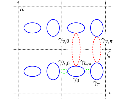
Figure 2. The adiabatic phase space

Consider an interval $J$ such that, for $E\in J$, the assumption on the relative position of the spectral window and the spectrum of $H_{0}$ described above is satisfied (see figure 1). Then, the curve $\Gamma_{\mathbb{R}}$ consists of a infinite union of connected components, each of which is homeomorphic to a torus ; there are exactly two such components in each periodicity cell, see figure 2. In this figure, each square represents a periodicity cell. The connected components of $\Gamma_{\mathbb{R}}$ are represented by full lines; we denote two of them by $\gamma_{0}$ and $\gamma_{\pi}$.
The dashed lines represent loops on $\Gamma$ that connect certain connected components of $\Gamma_{\mathbb{R}}$; one can distinguish between the “horizontal” loops and the “vertical” loops. There are two special horizontal loops denoted by $\gamma_{h,0}$ and $\gamma_{h,\pi}$; the loop $\gamma_{h,0}$ (resp. $\gamma_{h,\pi}$) connects $\gamma_{0}$ to $\gamma_{\pi}-(2\pi,0)$ (resp. $\gamma_{0}$ to $\gamma_{\pi}$). In the same way, there are two special vertical loops denoted by $\gamma_{v,0}$ and $\gamma_{v,\pi}$ ; the loop $\gamma_{v,0}$ (resp. $\gamma_{v,\pi}$) connects $\gamma_{0}$ to $\gamma_{0}+(0,2\pi)$ (resp. $\gamma_{\pi}$ to $\gamma_{\pi}+(0,2\pi)$).

The standard semi-classical heuristic suggests the following spectral behavior. To each of the loops $\gamma_{0}$ and $\gamma_{\pi}$, one associates a phase obtained by integrating the fundamental $1$-form on $\Gamma$ along the given loop; let $\Phi_{0}=\Phi_{0}(E)$ (resp. $\Phi_{\pi}=\Phi_{\pi}(E)$) be one half of the phase corresponding to $\gamma_{0}$ (resp. $\gamma_{\pi}$). Each of these phases defines a quantization condition

(0.5) $$\frac{1}{\varepsilon}\Phi_{0}(E)=\frac{\pi}{2}+n\pi\quad\quad\text{ and }\quad\quad\frac{1}{\varepsilon}\Phi_{\pi}(E)=\frac{\pi}{2}+n\pi,\quad\quad n\in{\mathbb{N}}.$$

Each of these conditions defines a sequence of energies in $J$, say $(E_{0}^{(l)})_{l}$ and $(E_{\pi}^{(l^{\prime})})_{l^{\prime}}$. For $\varepsilon$ sufficiently small, the spectrum of $H_{z,\varepsilon}$ in $J$ should then be located in a neighborhood of these energies.

Moreover, to each of the complex loops $\gamma_{h,0}$, $\gamma_{h,\pi}$, $\gamma_{v,0}$ and $\gamma_{v,\pi}$, one naturally associates an action obtained by integrating the fundamental $1$-form on $\Gamma$ along the loop. For $b\in\{0,\pi\}$ and $a\in\{v,h\}$, we denote by $S_{a,b}$ the action associated to $\gamma_{a,b}$ multiplied by $i/2$. For $E\in{\mathbb{R}}$, all these actions are real. One orients the loops so that they all be positive. Finally, we define tunneling coefficients as

$$t_{a,b}=e^{-S_{a,b}/\varepsilon},\quad b\in\{0,\pi\},\ a\in\{v,h\}.$$

When the real iso-energy curve consists in a single torus per periodicity cell (see [12]), the spectrum of $H_{z,\varepsilon}$ is contained in a sequence of intervals described as follows:

• each interval is neighboring a solution of the quantization condition;

• the length of the interval is of order the largest tunneling coefficient associated to the loop;

• the nature of the spectrum is determined by the ratio of the vertical tunneling coefficient to the horizontal one:

  • if this ratio is large, the spectrum is singular;

  • if the ratio is small, the spectrum is absolutely continuous.

In the present case, one must moreover take into account the possible interactions between the tori living in the same periodicity cell. Similarly to what happens in the standard “double well” case (see [14, 24, 15]), this effect only plays an important role when the two energies, generated each by one of the tori, are sufficiently close to each other. In this paper, we do not consider the case when these energies are “resonant”, i.e. coincide or are “too close” to one another, but we can “go” up to the case of exponentially close energies.

Let $E_{0}$ be an energy satisfying the quantization condition (0.5) defined by $\Phi_{0}$; let $\delta$ be the distance from $E_{0}$ to the sequence of energies satisfying the quantization condition (0.5) defined by $\Phi_{\pi}$. We now discuss the possible cases depending on this distance. Let us just add that, as the sequences of energies satisfying the quantization equation given by $\Phi_{0}$ or $\Phi_{\pi}$ play symmetric roles, in this discussion, the indexes $0$ and $\pi$ can be interchanged freely.

First, we assume that, for some fixed $n>1$, this distance is of order at least $\varepsilon^{n}$. In this case, near $E_{0}$, the states of the system don’t “see” the other lattice of tori, those obtained by translation of the torus $\gamma_{\pi}$; nor do they “feel” the associated tunneling coefficient $t_{v,\pi}$. Near $E_{0}$, everything is as if there was a single torus, namely a translate of $\gamma_{0}$, per periodicity cell. Near $E_{0}$, the spectrum of $H_{z,\varepsilon}$ is located in a interval of length of order of the largest of the tunneling coefficients $t_{v,0}$ and $t_{h}=t_{h,0}t_{h,\pi}$ (see section 1.3.3). And, the nature of the spectrum is determined by quotient $t_{v,0}/t_{h}$.
So, in the energy region not too close to solutions to both quantization conditions in (0.5), we see that the spectrum is contained in two sequences of exponentially small intervals. For each sequence, the nature of the spectrum is obtained from comparing the vertical to the horizontal tunneling coefficient for the torus generating the sequence. As the tunneling coefficients for both tori are roughly “independent” (see section 1.7.5), it may happen that the spectrum for one of the interval sequences be singular while it be absolutely continuous for the other sequence. If this is the case, one obtains numerous Anderson transitions i.e., thresholds separating a.c. spectrum from singular spectrum (see figure 5(b)).

Let us now assume that $\delta$ is exponentially small, i.e. of order $e^{-\eta/\varepsilon}$ for some fixed positive $\eta$ (not too large, see section 1.6). This means that we approach the case of resonant energies. Note that, this implies that there is exactly one energy $E_{\pi}$ satisfying (0.5) for $\Phi_{\pi}$ that is exponentially close to $E_{0}$; all other energies satisfying (0.5) for $\Phi_{\pi}$ are at least at a distance of order $\epsilon$ away from $E_{0}$.
Then, one can observe two new phenomena. First, there is a repulsion of $I_{0}$ and $I_{\pi}$, the intervals corresponding to $E_{0}$ and $E_{\pi}$ respectively containing spectrum. This phenomenon is similar to the splitting phenomenon observed in the double well problem (see [14, 24, 15]). Second, the interaction can change the nature of the spectrum: the spectrum that would be singular for intervals sufficiently distant from each other can become absolutely continuous when they are close to each other, see Fig. 5(a). To explain this phenomenon, assume, for simplicity, that $t_{v,0}$ and $t_{v,\pi}$, the “vertical” tunneling coefficients associated to the tori $\gamma_{0}$ and $\gamma_{\pi}$, are of the same order (in $\varepsilon$), i.e. $t_{v,0}\sim t_{v,\pi}\sim t_{v}$. Then, if $|E_{0}-E_{\pi}|\sim\varepsilon^{n}$, on each of the intervals $I_{0}$ and $I_{\pi}$, the nature of the spectrum is determined by the same ratio $t_{v}/t_{h}$. If $|E_{0}-E_{\pi}|\sim e^{-\eta/\varepsilon}$, the two arrays of tori begin to “feel” one another: they form an array for which the tori from both arrays play equivalent roles. In result, the “horizontal” tunneling becomes stronger: it appears that $t_{h}$ has to be replaced by the effective “horizontal” tunneling coefficient $t_{h,{\rm eff}}=t_{h}/\text{dist}(E_{0},E_{\pi})$, and the ratio $t_{v}/t_{h}$ has to be replaced by $t_{v}/t_{h,{\rm eff}}$. So, the singular spectrum on the intervals $I_{0}$ and $I_{\pi}$ “tends to turn” into absolutely continuous one.

There is one more case that will not be discussed in the present paper: it is the case when $\delta\sim e^{-\eta/\varepsilon}$ with no restriction on $\eta$ positive or, even, when $\delta$ vanishes. This is the case of strong resonances; it reveals interesting new spectral phenomena and is studied in detail in [7].

1. The results

We now state our assumptions and results in a precise way.

1.1. The periodic operator

This section is devoted to the description of elements of the spectral theory of one-dimensional periodic Schrödinger operator $H_{0}$ that we need to present our results. For more details and proofs we refer to section 6 and to [6, 13].

1.1.1. The spectrum of $H_{0}$

The spectrum of the operator $H_{0}$ defined in (0.2) is a union of countably many intervals of the real axis, say $[E_{2n+1},\,E_{2n+2}]$ for $n\in{\mathbb{N}}$ , such that

$$E_{1}<E_{2}\leq E_{3}<E_{4}\dots E_{2n}\leq E_{2n+1}<E_{2n+2}\leq\dots\,,$$

$$E_{n}\to+\infty,\quad n\to+\infty.$$

This spectrum is purely absolutely continuous. The points $(E_{j})_{j\in{\mathbb{N}}}$ are the eigenvalues of the self-adjoint operator obtained by considering the differential polynomial (0.2) acting in $L^{2}([0,2])$ with periodic boundary conditions (see [6]). The intervals $[E_{2n+1},\,E_{2n+2}]$, $n\in{\mathbb{N}}$, are the spectral bands, and the intervals $(E_{2n},\,E_{2n+1})$, $n\in{\mathbb{N}}^{*}$, the spectral gaps. When $E_{2n}<E_{2n+1}$, one says that the $n$-th gap is open; when $[E_{2n-1},E_{2n}]$ is separated from the rest of the spectrum by open gaps, the $n$-th band is said to be isolated.

From now on, to simplify the exposition, we suppose that

(O):

all the gaps of the spectrum of $H_{0}$ are open.

1.1.2. The Bloch quasi-momentum

Let $x\mapsto\psi(x,E)$ be a non trivial solution to the periodic Schrödinger equation $H_{0}\psi=E\psi$ such that, for some $\mu\in{\mathbb{C}}$, $\psi\,(x+1,E)=\mu\,\psi\,(x,E)$, $\forall x\in{\mathbb{R}}$. This solution is called a Bloch solution to the equation, and $\mu$ is the Floquet multiplier associated to $\psi$. One may write $\mu=\exp(ik)$; then, $k$ is the Bloch quasi-momentum of the Bloch solution $\psi$.

It appears that the mapping $E\mapsto k(E)$ is an analytic multi-valued function; its branch points are the points $E_{1}$, $E_{2}$, $E_{3}$, $\dots$, $E_{n}$, $\dots$. They are all of “square root” type.

The dispersion relation $k\mapsto{\mathbf{E}}(k)$ is the inverse of the Bloch quasi-momentum. We refer to section 6.1.2 for more details on $k$.

1.2. A “geometric” assumption on the energy region under study

Let us now describe the energy region where our study will be valid.

The spectral window centered at $E$, $\mathcal{F}(E)$, is the range of the mapping $\zeta\in{\mathbb{R}}\mapsto E-\alpha\cos(\zeta)$.

In the sequel, $J$ always denotes a compact interval such that, for some $n\in{\mathbb{N}}^{*}$ and for all $E\in J$, one has

(TIBM):

$[E_{2n},E_{2n+1}]\subset\dot{\mathcal{F}}(E)$ and ${\mathcal{F}}(E)\subset]E_{2n-1},E_{2n+2}[$.

where $\dot{\mathcal{F}}(E)$ is the interior of $\mathcal{F}(E)$ (see figure 1).
Actually, in the analysis, one has to distinguish between the cases $n$ odd and $n$ even. From now on, we assume that, in the assumption (TIBM), $n$ is even. The case $n$ odd is dealt with in the same way. The spectral results are independent of whether $n$ is even or odd.

Remark 1.1.

As all the spectral gaps of $H_{0}$ are assumed to be open, as their length tends to $0$ at infinity, and, as the length of the spectral bands goes to infinity at infinity, it is clear that, for any non vanishing $\alpha$, assumption (TIBM) is satisfied in any gap at a sufficiently high energy; it suffices that this gap be of length smaller than $2\alpha$.

1.3. The definitions of the phase integrals and the tunneling coefficients

We now give precise definitions of the phase integrals and the tunneling coefficients appearing in the introduction.

1.3.1. The complex momentum and its branch points

The phase integrals and the tunneling coeffi-

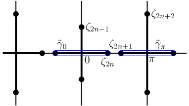
Figure 3. The branch points

cients are expressed in terms of integrals of the complex momentum. Fix $E$ in $J$. The complex momentum $\zeta\mapsto\kappa(\zeta)$ is defined by

(1.1) $$\hskip-142.26378pt\kappa(\zeta)=k(E-\alpha\cos(\zeta)).$$

As $k$, $\kappa$ is analytic and multi-valued. The set $\Gamma$ defined in (0.4) is the graph of the function $\kappa$. As the branch points of $k$ are the points $(E_{i})_{i\in{\mathbb{N}}}$, the branch points of $\kappa$ satisfy

(1.2) $$\hskip-142.26378ptE-\alpha\cos(\zeta)=E_{j},\ j\in{\mathbb{N}}^{*}.$$

As $E$ is real, the set of these points is symmetric with res-
pect to the real axis, to the imaginary axis; it is $2\pi$-periodic in $\zeta$. All the branch points of $\kappa$ lie in the set $\arccos({\mathbb{R}})$ which consists of the real axis and all the translates of the imaginary axis by a multiple of $\pi$.
As the branch points of the Bloch quasi-momentum, the branch points of $\kappa$ are of “square root” type. Due to the symmetries, it suffices to describe the branch points in the half-strip $\{\zeta;\ {\rm Im}\,\zeta\geq 0,\ 0\leq{\rm Re}\,\zeta\leq\pi\}$. These branch points are described in detail in section 7.1.1. In figure 3, we show some of them. The points $(\zeta_{j})_{j}$ satisfy (1.2); one has

$$0<\zeta_{2n}<\zeta_{2n+1}<\pi,\quad 0<{\rm Im}\,\zeta_{2n+2}<{\rm Im}\,\zeta_{2n+3}<\cdots,\quad 0<{\rm Im}\,\zeta_{2n-1}<\cdots<{\rm Im}\,\zeta_{1}.$$

1.3.2. The contours

To define the phases and the tunneling coefficients, we introduce some integration contours in the complex $\zeta$-plane.
These loops are shown in figure 3 and 4. The loops $\tilde{\gamma}_{0}$, $\tilde{\gamma}_{\pi}$, $\tilde{\gamma}_{h,0}$, $\tilde{\gamma}_{h,\pi}$, $\tilde{\gamma}_{v,0}$ and $\tilde{\gamma}_{v,\pi}$ are simple loops going once around respectively the intervals $[-\zeta_{2n},\zeta_{2n}]$, $[\zeta_{2n+1},2\pi-\zeta_{2n+1}]$, $[-\zeta_{2n+1},-\zeta_{2n}]$, $[\zeta_{2n},\zeta_{2n+1}]$, $[\zeta_{2n-1},\overline{\zeta_{2n-1}}]$ and $[\zeta_{2n+2},\overline{\zeta_{2n+2}}]$.
In section 10.1, we show that, on each of the above loops, one can fix a continuous branch of the complex momentum.
Consider $\Gamma$, the complex iso-energy curve defined by (0.4). Define the projection $\Pi:(\zeta,\kappa)\in\Gamma\mapsto\zeta\in{\mathbb{C}}$. The fact that, on each of the loops $\tilde{\gamma}_{0}$, $\tilde{\gamma}_{\pi}$, $\tilde{\gamma}_{h,0}$, $\tilde{\gamma}_{h,\pi}$, $\tilde{\gamma}_{v,0}$ and $\tilde{\gamma}_{v,\pi}$, one can fix a continuous branch of the complex momentum implies that each of these loops is the projection on the complex plane of some loop in $\Gamma$ i.e., for $\tilde{\gamma}\in\{\tilde{\gamma}_{0},\tilde{\gamma}_{\pi},\tilde{\gamma}_{h,0},\tilde{\gamma}_{h,\pi},\tilde{\gamma}_{v,0},\tilde{\gamma}_{v,\pi}\}$, there exists $\gamma\subset\Gamma$ such that $\tilde{\gamma}=\Pi(\gamma)$. In sections 10.6.1 and 10.6.2, we give the precise definitions of the curves $\gamma_{0}$, $\gamma_{\pi}$, $\gamma_{h,0}$, $\gamma_{h,\pi}$, $\gamma_{v,0}$ and $\gamma_{v,\pi}$ represented in figures 3 and 2 and show that they project onto the curves $\tilde{\gamma}_{0}$, $\tilde{\gamma}_{\pi}$, $\tilde{\gamma}_{h,0}$, $\tilde{\gamma}_{h,\pi}$, $\tilde{\gamma}_{v,0}$ and $\tilde{\gamma}_{v,\pi}$ respectively.

1.3.3. The phase integrals, the action integrals and the tunneling coefficients

The results described below are proved in section 10.

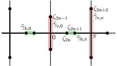
Figure 4. The loops for the phases

Let $\nu\in\{0,\pi\}$. To the loop $\gamma_{\nu}$, we associate the phase integral $\Phi_{\nu}$ defined as

(1.3) $$\hskip-142.26378pt\Phi_{\nu}(E)=\frac{1}{2}\oint_{\tilde{\gamma}_{\nu}}\kappa\,d\zeta,$$

where $\kappa$ is a branch of the complex momentum that is continuous on $\tilde{\gamma}_{\nu}$. The function $E\mapsto\Phi_{\nu}(E)$ is real analytic and does not vanish on $J$. The loop $\tilde{\gamma}_{\nu}$ is oriented so that $\Phi_{\nu}(E)$ be positive. One shows that, for all $E\in J$,

(1.4) $$\hskip-142.26378pt\quad\Phi_{0}^{\prime}(E)<0\quad\text{ and }\quad\Phi_{\pi}^{\prime}(E)>0.$$

To the loop $\gamma_{v,\nu}$, we associate the vertical action integral $S_{v,\nu}$ defined as

(1.5) $$\hskip-142.26378ptS_{v,\nu}(E)=-\frac{i}{2}\oint_{\tilde{\gamma}_{v,\nu}}\kappa d\zeta,$$

where $\kappa$ is a branch of the complex momentum that is continuous on $\tilde{\gamma}_{v,\nu}$. The vertical tunneling coefficient is defined to be

(1.6) $$t_{v,\nu}(E)=\exp\left(-\frac{1}{\varepsilon}S_{v,\nu}(E)\right).$$

The function $E\mapsto S_{v,\nu}(E)$ is real analytic and does not vanish on $J$. The loop $\tilde{\gamma}_{v,\nu}$ is oriented so that $S_{v,\nu}(E)$ be positive.

The index $\nu$ being chosen as above, we define horizontal action integral $S_{h,\nu}$ by

(1.7) $$S_{h,\nu}(E)=-\frac{i}{2}\oint_{\tilde{\gamma}_{h,\nu}}\kappa(\zeta)\,d\zeta,$$

where $\kappa$ is a branch of the complex momentum that is continuous on $\tilde{\gamma}_{h,\nu}$. The function $E\mapsto S_{h,\nu}(E)$ is real analytic and does not vanish on $J$. The loop $\tilde{\gamma}_{h,\nu}$ is oriented so that $S_{h,\nu}(E)$ be positive. The horizontal tunneling coefficient is defined as

(1.8) $$t_{h,\nu}(E)=\exp\left(-\frac{1}{\varepsilon}S_{h,\nu}(E)\right).$$

In section 10.4, we check that

(1.9) $$S_{h,0}(E)=S_{h,\pi}(E)\quad\text{ and }\quad t_{h,0}(E)=t_{h,\pi}(E).$$

One defines

(1.10) $$S_{h}(E)=S_{h,0}(E)+S_{h,\pi}(E)\quad\text{ and }\quad t_{h}(E)=t_{h,0}(E)\cdot t_{h,\pi}(E).$$

In (1.3), (1.5), and (1.7), only the sign of the integral depends on the choice of the branch of $\kappa$; this sign was fixed by orienting the integration contour; for more details, see sections 10.1 and 10.2.

1.4. Ergodic family

Before discussing the spectral properties of $H_{z,\varepsilon}$, we recall some general well known results from the spectral theory of ergodic operators.

As $2\pi/\varepsilon$ is supposed to be irrational, the function $x\mapsto V(x-z)+\alpha\cos(\varepsilon x)$ is quasi-periodic in $x$, and the operators defined by (0.1) form an ergodic family (see [22]).

The ergodicity implies the following consequences:

1. the spectrum of $H_{z,\varepsilon}$ is almost surely independent of $z$ ([1, 23]);

2. the absolutely continuous spectrum and the singular spectrum are almost surely independent of $z$ ([23, 18]);

3. the discrete spectrum is empty ([23]);

4. the Lyapunov exponent exists for almost all $z$ and is independent of $z$ ([23]); it is defined in the following way: let $x\mapsto\psi(x)$ be the solution to the Cauchy problem

   $$H_{z,\varepsilon}\psi=E\psi,\quad\psi_{|x=0}=0,\quad\psi^{\prime}_{|x=0}=1,$$

   the following limit (when it exists) defines the Lyapunov exponent:

   $$\Theta(E)=\Theta(E,\varepsilon):=\lim_{x\to+\infty}\frac{\log\left(\sqrt{|\psi(x,E,z)|^{2}+|\psi^{\prime}(x,E,z)|^{2}}\right)}{|x|}.$$

5. the absolutely continuous spectrum is the essential closure of the set of $E$ where $\Theta(E)=0$ (the Ishii-Pastur-Kotani Theorem, see [23]);

6. the density of states exists for almost all $z$ and is independent of $z$ ([23]); it is defined in the following way: for $L>0$, let $H_{z,\varepsilon;L}$ be the operator $H_{z,\varepsilon}$ restricted to the interval $[-L,L]$ with the Dirichlet boundary conditions; for $E\in{\mathbb{R}}$; the following limit (when it exists) defines the density of states:

   $$N(E)=N(E,\varepsilon):=\lim_{L\to+\infty}\frac{\#\{\text{ eigenvalues of }H_{z,\varepsilon;L}\text{less then or equal to}E\}}{2L};$$

7. the density of states is non decreasing; the spectrum of $H_{z,\varepsilon}$ is the set of points of increase of the density of states.

1.5. A coarse description of the location of the spectrum in $J$

Henceforth, we assume that the assumptions (H) and (O) are satisfied and that $J$ is a compact interval satisfying (TIBM). Moreover, we suppose that

(T):

$\displaystyle 2\pi\cdot\min_{E\in J}\min({\rm Im}\,\zeta_{2n-2}(E),\,{\rm Im}\,\zeta_{2n+3}(E))>\max_{E\in J}\max(S_{h}(E),\,S_{v,0}(E),\,S_{v,\pi}(E))$.

Note that (T) is verified if the spectrum of $H_{0}$ has two successive bands that are sufficiently close to each other and sufficiently far away from the remainder of the spectrum (this can be checked numerically on simple examples, see section 1.8). In section 1.9, we will discuss this assumption further.

Define

(1.11) $$\delta_{0}:=\frac{1}{2}\inf_{E\in J}\min(S_{h}(E),S_{v,0}(E),S_{v,\pi}(E))>0.$$

We prove

Theorem 1.1.

Fix $E_{*}\in J$. For $\varepsilon$ sufficiently small, there exists $V_{*}\subset{\mathbb{C}}$, a neighborhood of $E_{*}$, and two real analytic functions $E\mapsto\check{\Phi}_{0}(E,\varepsilon)$ and $E\mapsto\check{\Phi}_{\pi}(E,\varepsilon)$, defined on $V_{*}$ satisfying the uniform asymptotics

(1.12) $$\check{\Phi}_{0}(E,\varepsilon)=\Phi_{0}(E)+o(\varepsilon),\quad\check{\Phi}_{\pi}(E,\varepsilon)=\Phi_{\pi}(E)+o(\varepsilon)\quad\text{where }\sup_{E\in V_{*}}|\varepsilon^{-1}o(\varepsilon)|\operatornamewithlimits{\to}_{\varepsilon\to 0}0,$$

such that, if one defines two finite sequences of points in $J\cap V_{*}$, say $(E_{0}^{(l)})_{l}:=(E_{0}^{(l)}(\varepsilon))_{l}$ and $(E_{\pi}^{(l^{\prime})})_{l^{\prime}}:=(E_{\pi}^{(l^{\prime})}(\varepsilon))_{l^{\prime}}$, by

(1.13) $$\frac{1}{\varepsilon}\check{\Phi}_{0}(E_{0}^{(l)},\varepsilon)=\frac{\pi}{2}+\pi l\quad\text{ and }\quad\frac{1}{\varepsilon}\check{\Phi}_{\pi}(E_{\pi}^{(l^{\prime})},\varepsilon)=\frac{\pi}{2}+\pi l^{\prime},\quad(l,\,l^{\prime})\in{\mathbb{N}}^{2},$$

then, for all $z$, the spectrum of $H_{z,\varepsilon}$ in $J\cap V_{*}$ is contained in the union of the intervals

$$I_{0}^{(l)}:=E_{0}^{(l)}+[-e^{-\delta_{0}/\varepsilon},e^{-\delta_{0}/\varepsilon}]\quad\text{ and }\quad I_{\pi}^{(l^{\prime})}:=E_{\pi}^{(l^{\prime})}+[-e^{-\delta_{0}/\varepsilon},e^{-\delta_{0}/\varepsilon}]$$

that is

$$\sigma(H_{z,\varepsilon})\cap J\cap V_{*}\subset\left(\bigcup_{l}I_{0}^{(l)}\right)\bigcup\left(\bigcup_{l^{\prime}}I_{\pi}^{(l^{\prime})}\right).$$

In the sequel, to alleviate the notations, we omit the reference to $\varepsilon$ in the functions $\check{\Phi}_{0}$ and $\check{\Phi}_{\pi}$.

By (1.4) and (1.12), there exists $C>0$ such that, for $\varepsilon$ sufficiently small, the points defined in (1.13) satisfy

(1.14) $$\frac{1}{C}\varepsilon\leq E_{0}^{(l)}-E_{0}^{(l-1)}\leq C\varepsilon,$$

(1.15) $$\frac{1}{C}\varepsilon\leq E_{\pi}^{(l)}-E_{\pi}^{(l-1)}\leq C\varepsilon.$$

Moreover, for $\nu\in\{0,\pi\}$, in the interval $J\cap V_{*}$, the number of points $E_{\nu}^{(l)}$ is of order $1/\varepsilon$.

In the sequel, we refer to the points $E_{0}^{(l)}$ (resp. $E_{\pi}^{(l)}$), and, by extension, to the intervals $I_{0}^{(l)}$ (resp. $I_{\pi}^{(l)}$) attached to them, as of type $0$ (resp. type $\pi$).

By (1.14) and (1.15), the intervals of type $0$ (resp. $\pi$) are two by two disjoints; any interval of type $0$ (resp. $\pi$) intersects at most a single interval of type $\pi$ (resp. $0$).

1.6. A precise description of the location of the spectrum in $J$

We now describe the spectrum of $H_{z,\varepsilon}$ in the intervals defined in Theorem 1.1. Let us assume the interval under consideration is of type $\pi$. One needs to distinguish two cases whether this interval intersects or not an interval of type $0$. The intervals of one of the families that do not intersect any interval of the other family are called non-resonant, the others being the resonant intervals.

In the present paper, we only study the non-resonant intervals; the resonant one are studied in [7]. The non-resonant is the simplest of the two cases; nevertheless, one already sees that new spectral phenomena occur.

Remark 1.2.

One may wonder whether resonances occur. They do occur. Recall that the derivatives of $\Phi_{\pi}$ and $\Phi_{0}$ are of opposite signs on $J$, see (1.4). Hence, as $\varepsilon$ decreases, on $J$, the points of type $0$ and $\pi$ move toward each other (at least, in the leading order in $\varepsilon$). The motion being continuous, they meet.

Nevertheless, for a generic $V$, there are only a few resonant intervals in $J$. On the other hand, for symmetric $V$, there may be numerous resonant energies; e.g., if $V$ is even, then the sequences $(E_{0}^{(l)})_{l}$ and $(E_{\pi}^{(l^{\prime})})_{l^{\prime}}$ coincide and all the intervals are resonant! This is due to the fact that the cosine is even; it is not true if $\alpha\cos(\cdot)$ is replaced by a generic potential.

We will describe our results for the intervals of type $\pi$; mutandi mutandis, the results for the intervals of type $0$ are the same. One has

Theorem 1.2.

Assume the conditions of Theorem 1.1 are satisfied. For $\varepsilon$ sufficiently small, let $(I_{0}^{(l^{\prime})})_{l^{\prime}}$ and $(I_{\pi}^{(l)})_{l}$ be the finite sequences of intervals defined in Theorem 1.1. Consider $l$ such that, for any $l^{\prime}$, $I_{\pi}^{(l)}\cap I_{0}^{(l^{\prime})}=\emptyset$. Then, the spectrum of $H_{z,\varepsilon}$ in $I_{\pi}^{(l)}$ is contained $\check{I}_{\pi}^{(l)}$, the interval centered at the point

(1.16) $$\check{E}_{\pi}^{(l)}=E_{\pi}^{(l)}+\varepsilon\,\frac{\Lambda_{n}(V)}{2\check{\Phi}_{\pi}^{\prime}(E_{\pi}^{(l)})}\,t_{h}(E_{\pi}^{(l)})\,\tan\left(\frac{\check{\Phi}_{0}(E_{\pi}^{(l)})}{\varepsilon}\right),$$

and of length

(1.17) $$\left|\check{I}_{\pi}^{(l)}\right|=\frac{2\varepsilon}{\check{\Phi}_{\pi}^{\prime}(E_{\pi}^{(l)})}\left(\frac{t_{h}(E_{\pi}^{(l)})}{2\left|\cos\left(\frac{\check{\Phi}_{0}(E_{\pi}^{(l)})}{\varepsilon}\right)\right|}+t_{v,\pi}(E_{\pi}^{(l)})\right)\,(1+o(1)).$$

The factor $\Lambda_{n}(V)$ is positive, and depends only on $V$ and on $n$ (see section 6.2.1).
In (1.17), $o(1)$ tends to $0$ when $\varepsilon$ tends to $0$, uniformly in $E\in\check{I}_{\pi}^{(l)}$ and $l$ such that, for any $l^{\prime}$, $I_{\pi}^{(l)}\cap I_{0}^{(l^{\prime})}=\emptyset$.

The fact that each of the intervals $\check{I}_{\pi}^{(l)}$ does contain some spectrum follows from

Theorem 1.3.

Let $dN_{\varepsilon}(E)$ denote the density of states measure of $H_{z,\varepsilon}$. In the case of Theorem 1.2, for any $l$, one has

$$\int_{\check{I}_{\pi}^{(l)}}dN_{\varepsilon}(E)=\frac{\varepsilon}{2\pi}.$$

“Level repulsion”.  Let $E_{0}$ be the point in the sequence $(E_{0}^{(l^{\prime})})_{l^{\prime}}$ closest to $E_{\pi}:=E_{\pi}^{(l)}$. Analyzing formulae (1.16) and (1.17), one notices a repulsion between the intervals $\check{I}_{0}$ and $\check{I}_{\pi}$.
Indeed, consider the second term in the right hand side of (1.16). As $\check{\Phi}_{\pi}^{\prime}(E)>0$, this term has the same sign as $\tan\left(\frac{\check{\Phi}_{0}(E_{\pi})}{\varepsilon}\right)$. Assume that $E_{0}$ and $E_{\pi}$ are sufficiently close to each other. As, by definition, $\displaystyle\frac{1}{\varepsilon}\check{\Phi}_{0}(E_{0})=\frac{\pi}{2}$ mod $\pi$ and as $\check{\Phi}_{0}^{\prime}(E)<0$, the second term in the right hand side of (1.16) is negative (resp. positive) if $E_{\pi}$ is to the left (resp. right) of $E_{0}$. So, there is a repulsion between $\check{I}_{0}$ and $\check{I}_{\pi}$. As the distance from $E_{\pi}$ to $E_{0}$ controls the factor

$$\cos\left(\frac{\check{\Phi}_{0}(E_{\pi})}{\varepsilon}\right),$$

the smaller this distance, the larger the repulsion.

1.7. The Lyapunov exponent and the nature of the spectrum in $J$

Here, we discuss the nature of the spectrum in the interval $\check{I}_{\pi}^{(l)}$. Therefore, we define

(1.18) $$\lambda_{\pi}(E)=\frac{t_{v,\pi}(E)}{t_{h}(E)}\,{\rm dist}\,\left(E,\bigcup_{l^{\prime}}\{E_{0}^{(l^{\prime})}\}\right),$$

where, for a set $A$, ${\rm dist}\,(E,A)$ denotes the Euclidean distance from $E$ to $A$.

1.7.1. The Lyapunov exponent

We prove

Theorem 1.4.

On the interval $\check{I}_{\pi}^{(l)}$, the Lyapunov exponent has the following asymptotic

(1.19) $$\Theta(E,\varepsilon)=\frac{\varepsilon}{2\pi}\log^{+}\lambda_{\pi}(E_{\pi}^{(l)})+o(1),$$

where $o(1)$ tends to $0$ when $\varepsilon$ tends to $0$, uniformly in $E\in\check{I}_{\pi}^{(l)}$ and $l$ such that, for any $l^{\prime}$, $I_{\pi}^{(l)}\cap I_{0}^{(l^{\prime})}=\emptyset$. Here, $\log^{+}=\max(0,\log)$.

1.7.2. Sharp drops of the Lyapunov exponent due to the resonance interaction

Formula (1.19) shows that the Lyapunov exponent becomes “abnormally small” on the interval $\check{I}_{\pi}^{(l)}$ when it becomes close to one of the points $\{E_{0}^{(l^{\prime})}\}$. Let us discuss this in more details.
Assume that $(S_{h}-S_{v,\pi})(E_{\pi}^{(l)})>0$. If ${\rm dist}\,\left(E_{\pi}^{(l)},\bigcup_{l}\{E_{0}^{(l^{\prime})}\}\right)\geq\varepsilon^{N}$ (where $N$ is a fixed positive integer) then, Theorem 1.4 and formula (1.18) imply that

$$\Theta(E,\varepsilon)=\frac{1}{2\pi}(S_{h}-S_{v,\pi})(E_{\pi}^{(l)})+o(1)\text{ when }\varepsilon\to 0.$$

On the other hand, when $E_{\pi}^{(l)}$ is only at a distance of size $e^{-\delta/\varepsilon}$ (for $0<\delta<(S_{h}-S_{v,\pi})^{+}$) from the set of energies $\{E_{0}^{(l^{\prime})}\}$, on $\check{I}_{\pi}^{(l)}$, one has

$$\Theta(E,\varepsilon)=\frac{1}{2\pi}\left[(S_{h}-S_{v,\pi})(E_{\pi}^{(l)})-\delta\right]+o(1)\text{ when }\varepsilon\to 0.$$

Hence, the value of $\Theta$ on $\check{I}_{\pi}^{(l)}$ drops sharply when $E_{\pi}^{(l)}$ approaches the sequence $(E_{0}^{(l^{\prime})})_{l^{\prime}}$.

1.7.3. Singular spectrum

As a natural consequence of Theorem 1.4 and the Ishii-Pastur-Kotani Theorem [23], we obtain the

Corollary 1.1.

Fix $c>0$. For $\varepsilon$ sufficiently small, if $I_{\pi}^{(l)}$ is non-resonant and if $\varepsilon\log\lambda_{\pi}(E_{\pi}^{(l)})>c$, then, the interval $\check{I}_{\pi}^{(l)}$ defined in Theorem 1.2 only contains singular spectrum.

1.7.4. Absolutely continuous spectrum

If $\lambda_{\pi}$ is small on the interval $\check{I}_{\pi}^{(l)}$, most of this interval is made of absolutely continuous spectrum; one shows

Theorem 1.5.

For $c>0$, there exists $\eta$, a positive constant, and a set of Diophantine numbers $D\subset(0,1)$ such that

• asymptotically, $D$ has total measure i.e.

  (1.20) $$\frac{{\rm mes}\,(D\cap(0,\varepsilon))}{\varepsilon}=1+e^{-\eta/\varepsilon}o\left(1\right).$$

• for $\varepsilon\in D$ sufficiently small, if $\check{I}_{\pi}^{(l)}$ is non-resonant and if $\varepsilon\log\lambda_{\pi}(E_{\pi}^{(l)})<-c$, then, one has

  (1.21) $$\frac{{\rm mes}\,(\check{I}_{\pi}^{(l)}\cap\Sigma_{\rm ac})}{{\rm mes}\,(\check{I}_{\pi}^{(l)})}=1+o(1),$$

  and $\Sigma_{ac}$ denotes the absolutely continuous spectrum of $H_{z,\varepsilon}$.
  In (1.20) and (1.21), $o(1)$ tends to $0$ when $\varepsilon$ tends to $0$, uniformly in $E\in\check{I}_{\pi}^{(l)}$ and $l$ such that, for any $l^{\prime}$, $I_{\pi}^{(l)}\cap I_{0}^{(l^{\prime})}=\emptyset$.

1.7.5. A remark

The nature of the spectrum depends on the interplay between the values of the actions $S_{h}$, $S_{v,0}$, $S_{v,\pi}$. So, when analyzing our results, it is helpful to keep in mind the following observation. As underlined at the end of section 1.5, choosing $\varepsilon$ carefully, one can arrange that the distance between the sequences of energies of type $0$ and $\pi$ be arbitrarily small; moreover, this can be done in any compact subinterval of $J$ of length at least $C\varepsilon$ (if $C$ is chosen sufficiently large). On such an interval, the actions $E\mapsto S_{h}(E)$, $E\mapsto S_{v,0}(E)$ and $E\mapsto S_{v,\pi}(E)$ vary at most of $C^{\prime}\varepsilon$. Hence, at the expense of choosing $\varepsilon$ sufficiently small in the right way, we may essentially suppose that there exists an energy of type $0$ and one of type $\pi$ at an arbitrarily small distance from each other such that, on an $\varepsilon$-neighborhood of these points, the triple $E\mapsto(S_{h}(E),S_{v,0}(E),S_{v,\pi}(E))$ takes any of its possible values on $J$. This means that one can pick the values of $E_{\pi}^{(l^{\prime})}-E_{0}^{(l)}$ and $(S_{h}(E),S_{v,0}(E),S_{v,\pi}(E))$ essentially independently of each other.

Now, let us discuss two new spectral phenomena that can occur under the hypothesis (TIBM).

1.7.6. Transitions due to the proximity to a resonance

The nature of the spectrum on the intervals defined in Theorem 1.2 depends on their distance to the intervals of the other family. The interaction can be strong enough to actually change the nature of the spectrum. Let us consider a simple example. Assume the interval $J$ satisfies:

(1.22) $$\min_{E\in J}S_{h}(E)>\max_{\nu\in\{0,\pi\}}\max_{E\in J}S_{v,\nu}(E),$$

and

(1.23) $$\frac{3}{2}\min_{\nu\in\{0,\pi\}}\min_{E\in J}S_{v,\nu}(E)>\max_{E\in J}S_{h}(E).$$

Condition (1.22) guarantees that $\displaystyle\delta_{0}=\frac{1}{2}\,\min_{\nu\in\{0,\pi\}}\min_{E\in J}S_{v,\nu}(E)$. Hence, there exists $c>0$ such that, for $E\in J$ and $\nu\in\{0,\pi\}$,

(1.24) $$S_{h}(E)-S_{v,\nu}(E)-\delta_{0}<-c<0.$$

Consider now $I_{0}^{(l^{\prime})}$ and $I_{\pi}^{(l)}$ both non resonant located in $J\cap V_{*}$. Then,

• if the two intervals are distant of at least $\varepsilon^{N}$ (where $N$ is a fixed integer) from each other, condition (1.22) guarantees that, on these intervals, the spectrum is controlled by Corollary 1.1 and its analogue for the intervals of type $0$.

• if the two intervals are distant of $C\exp\left(-\delta_{0}/\varepsilon\right)$ from each other, then condition (1.24) guarantees that, on these intervals, the spectrum is controlled by Theorem 1.5 and its analogue for the intervals of type $0$.

That intervals $J$ where both (1.22) and (1.23) hold exist can be checked numerically, see section 1.8. Thus, not only does the location of the spectrum depend of the distance separating intervals of type $0$ for neighboring intervals of type $\pi$, but so does also the nature of the spectrum. Transition can occur due to this interaction phenomenon: spectrum that would be singular were the intervals sufficiently distant from each other can become absolutely continuous when they are close to each other (see Fig. 5(a)).

1.7.7. Alternating spectra

To describe this phenomenon, to keep things simple, assume that, in $V_{*}\cap J$, the distance between the points $\{E_{0}^{(l)}\}$ and the points $\{E_{\pi}^{(l^{\prime})}\}$ is larger than $\varepsilon^{N}$ (for some fixed $N$); hence, all energies are non-resonant in $V_{*}\cap J$. Taking Theorem 1.5 and Corollary 1.1 into account, we see that, on $\check{I}_{0}^{(l)}$ (resp. $\check{I}_{\pi}^{(l^{\prime})}$), the nature of the spectrum is determined by the size of the ratio $t_{v,0}(E_{0}^{(l)})/t_{h}(E_{0}^{(l)})$ (resp. $t_{v,\pi}(E_{\pi}^{(l^{\prime})})/t_{h}(E_{\pi}^{(l^{\prime})})$). So, if for some $\delta>0$, one has

(1.25) $$\forall E\in J\cap V_{*},\quad S_{v,\pi}(E)-S_{h}(E)>\delta\quad\text{ et }\quad S_{v,0}(E)-S_{h}(E)<-\delta,$$

then, in $V_{*}\cap J$, the sequences of type $0$ and $\pi$ contain spectra of “opposite” nature: the spectrum in the intervals of type $0$ is singular, and that in the intervals of type $\pi$ is, mostly, absolutely continuous. This holds under the Diophantine condition on $\varepsilon$ spelled out in Theorem 1.5. Hence, one obtains an interlacing of intervals containing spectra of “opposite” types, see Fig. 5(b). In this case, the number of Anderson transitions in $V_{*}\cap J$ is of order $1/\varepsilon$.
One can check numerically that the condition (1.25) is fulfilled for some energy region $V_{*}$ and some values of $\alpha$ (see section 1.8).

(a) Almost resonant transitions

(b) Alternating spectra

Figure 5. Two new spectral phenomena

1.8. Numerical computations

We now turn to numerical results showing that the multiple phenomena described in sections 1.7.6 and 1.7.7 do occur.

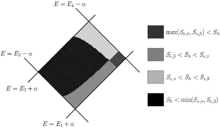
Figure 6. Comparing the actions

All these phenomena only depend on the values of the actions $S_{h}$, $S_{v,0}$, $S_{v,\pi}$. For special potentials $V$, they are quite easy to compute numerically.

We pick $V$ to be a two-gap potential; for these potentials, the Bloch quasi-momentum $k$ (see section 1.1.2) is explicitly given by a hyper-elliptic integral ([17, 20]). The actions then become easily computable. As the spectrum of $H_{0}=-\Delta+V$ only has two gaps, we write $\sigma(H_{0})=[E_{1},E_{2}]\cup[E_{3},E_{4}]\cup[E_{5},+\infty[$. In the computations, we take the values

$$E_{1}=0,\ E_{2}=3.8571429,\ E_{3}=6.8571429,\ E_{4}=12.100395,\text{ and }E_{5}=100.70923.$$

On the figure 6, we represented the part of the $(\alpha,E)$-plane where the condition (TIBM) is satisfied for $n=1$. Its boundary consists of the straight lines $E=E_{1}+\alpha$, $E=E_{2}+\alpha$, $E=E_{3}-\alpha$ and $E=E_{4}-\alpha$. Denote it by $\Delta$.
The computations show that (T) is satisfied in the whole of $\Delta$. As $n=1$, one has $E_{2n-2}=-\infty$. So, it suffices to check (T) for $\zeta_{2n+3}=\zeta_{5}$. (T) can then be understood as a consequence of the fact that $E_{5}-E_{4}$ is large.
On the figure 6, one sees that, for non-resonant intervals,

• the zones where one has alternating spectral types (see section 1.7.7) are those where either $S_{v,0}<S_{h}<S_{v,\pi}$ or $S_{v,\pi}<S_{h}<S_{v,0}$

• the transitions due to the proximity of the resonant situation (see section 1.7.6) take place in the part of region $\{S_{h}>\max(S_{v,\pi},S_{v,0})\}$ sufficiently close to $\{S_{h}<\min(S_{v,\pi},S_{v,0})\}$.

1.9. Comments, generalizations and remarks

About assumption (T), its purpose is to select which tunneling coefficients play the main role in the spectral behavior of $H_{z,\varepsilon}$ in the interval $J$; this assumptions guarantees that it is the tunneling coefficients associated to the loops defined in section 1.3.2 that give rise to the principal terms in the asymptotics of the monodromy matrix that we describe in section 2.

In the present paper, we restricted ourselves to perturbations of $H_{0}$ of the form $\alpha\cos$. As will be seen from the proofs, this is not necessary. The essential special features of the cosine that were used are the simplicity of its reciprocal function (that is multivalued on ${\mathbb{C}}$). More precisely, the assumption that is really needed is that the geometry of the objects of the complex WKB method that is used to compute the asymptotics of the monodromy matrix be as simple as that for the cosine. This geometry does not only depend on the perturbation; it also depends on the interval $J$ under consideration and on the Bloch quasi-momentum of $H_{0}$. The precise assumptions needed to have our analysis work are requirements on the conformal properties of the complex momentum.

The methods developed in [11, 12, 8, 9, 10] are quite general; using them, one can certainly analyze more complicated situations i.e., more general adiabatic perturbations of $H_{0}$. Nevertheless, the computations may become much more complicated than those found in the present paper.

1.10. Asymptotic notations

We now define some notations that will be used throughout the paper. Below $C$ denotes different positive constants independent of $\varepsilon$, $E$ and $E_{\pi}$.
When writing $f=O(g)$, we mean that there exits $C>0$ such that $|f|\leq C\,|g|$ for all $\varepsilon$, $z$, $E$ in consideration.
When writing $f=o(g)$, we mean that there exists $\varepsilon\mapsto c(\varepsilon)$, a function such that

• $|f|\leq c(\varepsilon)|g|$ for all $\varepsilon$, $z$, $E$ in consideration;

• $c(\varepsilon)\to 0$ when $\varepsilon\to 0$.

When writing $f\asymp g$, we mean that there exists $C>1$ such that $C^{-1}|g|\leq|f|\leq C|g|$ for all $\varepsilon$, $z$, $E$ in consideration.
When writing error estimates, the symbol $O(f_{1},f_{2},\dots f_{n})$ denotes functions satisfying the estimate

(1.26) $$|O(f_{1},f_{2},\dots f_{n})|\leq C(|f_{1}|+|f_{2}|+\dots|f_{n}|),$$

with a positive constant $C$ independent of $z$, $E$ and $\varepsilon$ under consideration.

2. The monodromy matrix

In this section, we consider the quasi-periodic differential equation

(2.1) $$-\frac{d^{2}}{dx^{2}}\psi(x)+(V(x-z)+\alpha\cos(\varepsilon x))\psi(x)=E\psi(x),\quad x\in{\mathbb{R}},$$

and recall the definition of the monodromy matrix and of the monodromy equation for (2.1). We also recall how these objects are related to the spectral theory of the operator $H_{z,\varepsilon}$ defined in (0.1). Finally, we describe two monodromy matrices for (2.1).

2.1. The monodromy matrices and the monodromy equation

We now follow [11, 12], where the reader can find more details, results and their proofs.

2.1.1. The definition of the monodromy matrix

For any $z$ fixed, let $(\psi_{j}(x,\,z))_{j\in\{1,2\}}$ be two linearly independent solutions of equation (2.1). We say that they form a consistent basis if their Wronskian is independent of $z$, and, if for $j\in\{1,2\}$ and all $x$ and $z$,

(2.2) $$\psi_{j}(x,\,z+1)=\psi_{j}(x,\,z).$$

As $(\psi_{j}(x,\,z))_{j\in\{1,2\}}$ are solutions to equation (2.1), so are the functions $((x,z)\mapsto\psi_{j}(x+2\pi/\varepsilon,z+2\pi/\varepsilon))_{j\in\{1,2\}}$. Therefore, one can write

(2.3) $$\Psi\,(x+2\pi/\varepsilon,z+2\pi/\varepsilon)=M\,(z,E)\,\Psi\,(x,z),\quad\Psi(x,z)=\begin{pmatrix}\psi_{1}(x,\,z)\\ \psi_{2}(x,z)\end{pmatrix},$$

where $M\,(z,E)$ is a $2\times 2$ matrix with coefficients independent of $x$. The matrix $M(z,E)$ is called the monodromy matrix corresponding to the basis $(\psi_{j})_{j\in\{1,2\}}$. To simplify the notations, we often drop the $E$ dependence when not useful.

For any consistent basis, the monodromy matrix satisfies

(2.4) $$\det M\,(z)=1,\quad M\,(z+1)=M\,(z),\quad\forall z.$$

2.1.2. The monodromy equation and the link with the spectral theory of $H_{z,\varepsilon}$

Set

(2.5) $$h=\frac{2\pi}{\varepsilon}\,{\rm mod}\,1.$$

Let $M$ be the monodromy matrix corresponding to the consistent basis $(\psi_{j})_{j=1,2}$. Consider the monodromy equation

(2.6) $$F(n+1)=M\,(z+nh)F(n),\quad\text{where}\quad F(n)\in{\mathbb{C}}^{2},\quad\forall n\in{\mathbb{Z}}.$$

The spectral properties of $H_{z,\varepsilon}$ defined in (0.1) are tightly related to the behavior of solutions of (2.6). For now we will give a simple example of this relation; more examples will be given in the course of the paper.

Recall the definition of the Lyapunov exponent for a matrix cocycle. Let $z\mapsto M(z)$ be an $SL({\mathbb{C}},\,2)$-valued $1$-periodic function of the real variable $z$. Let $h$ be a positive irrational number. The Lyapunov exponent for the matrix cocycle $(M,h)$ is the the limit (when it exists)

(2.7) $$\theta(M,h)=\lim_{L\to+\infty}\frac{1}{L}\log\|M(z+Lh)\cdot M(z+(L-1)h)\cdots M(z+h)\cdot M(z)\|.$$

Actually, if $M$ is sufficiently regular in $z$ (say, if it belongs to $L^{\infty}$), then $\theta(M,h)$ exists for almost every $z$ and does not depend on $z$, see e.g. [23].

One has

Theorem 2.1 ([11]).

Let $h$ be defined by (2.5). Let $z\mapsto M(z,E)$ be a monodromy matrix for equation (2.1) corresponding to basis solutions that are locally bounded in $(x,z)$ together with their derivatives in $x$.
The Lyapunov exponents $\Theta(E,\varepsilon)$ and $\theta(M(\cdot,E),h)$ satisfy the relation

(2.8) $$\Theta(E,h)=\frac{\varepsilon}{2\pi}\theta(M(\cdot,E),h).$$

2.2. Asymptotics of two monodromy matrices

Recall that, in the interval $J$, the spectrum of $H_{z,\varepsilon}$ is contained in two sequences of subintervals of $J$, see Theorem 1.1. So, we consider two monodromy matrices, one for each sequence; for $\nu\in\{0,\pi\}$, the monodromy matrix $M_{\nu}$ is used to study the spectrum located near the points $(E_{\nu}^{(l)})_{l}$.
In this section, we first describe the monodromy matrix $M_{\pi}$ in detail. Then, we briefly discuss the monodromy matrix $M_{0}$.

Fix $\nu\in\{0,\pi\}$. The monodromy matrix $M_{\nu}$ is analytic in $z$ and $E$ and has the following structure:

(2.9) $$M_{\nu}=\begin{pmatrix}A_{\nu}&B_{\nu}\\ B_{\nu}^{*}&A_{\nu}^{*}\end{pmatrix}.$$

where, for $(z_{1},\cdots,z_{n})\mapsto g(z_{1},\cdots,z_{n})$, an analytic function, we have defined

(2.10) $$g^{*}(z_{1},\cdots,z_{n})=\overline{g(\overline{z_{1}},\cdots,\overline{z_{n}})}.$$

When describing the asymptotics of the monodromy matrices, we use the following notations:

• for $Y>0$, we let

  (2.11) $$T_{Y}=e^{-2\pi Y/\varepsilon};$$

• we put

  (2.12) $$p(z)=e^{2\pi|{\rm Im}\,z|}.$$

One has

Theorem 2.2.

There exists $V_{*}$, a complex neighborhood of $E_{*}$, such that, for sufficiently small $\varepsilon$, the following holds. Let

(2.13) $$Y_{m}=\frac{1}{2\pi}\inf_{E\in J\cap V_{*}}\max(S_{v,0}(E),S_{v,\pi}(E)),\quad\quad Y_{M}=\frac{1}{2\pi}\sup_{E\in J\cap V_{*}}\max(S_{v,0}(E),S_{v,\pi}(E),S_{h}(E)).$$

There exists $Y>Y_{M}$ and a consistent basis of solutions of (2.1) for which the monodromy matrix $(z,E)\mapsto M_{\pi}(z,E)$ is analytic in the domain $\left\{z\in{\mathbb{C}}:\,|{\rm Im}\,z|<\frac{Y}{\varepsilon}\right\}\times V_{*}$ and has the form (2.9).
Fix $0<y<Y_{m}$. Let $V_{*}^{\varepsilon}=\left\{E\in V_{*}:\,\,|{\rm Im}\,E|<\varepsilon\right\}$. In the domain

(2.14) $$\left\{z\in{\mathbb{C}}:\,|{\rm Im}\,z|<\frac{y}{\varepsilon}\right\}\times V_{*}^{\varepsilon},$$

the coefficients of $M_{\pi}$ admit the asymptotic representations:

(2.15) $$A_{\pi}=2\,\frac{\alpha_{\pi}e^{\frac{i\check{\Phi}_{\pi}}{\varepsilon}}\,C_{0}}{T_{h}}+\frac{1}{2}\,e^{\frac{i(\check{\Phi}_{\pi}-\check{\Phi}_{0})}{\varepsilon}}\,\left(\frac{1}{\theta}+\theta\right)+O\left(T_{h},\,\frac{T_{Y}p(z)}{T_{h}},\,T_{v,0}p(z),\,T_{v,\pi}p(z)\right)$$

and

(2.16) $$B_{\pi}=2\,\frac{\alpha_{\pi}e^{\frac{i\check{\Phi}_{\pi}}{\varepsilon}}\,C_{0}}{T_{h}}+\frac{1}{2}\,e^{\frac{i\check{\Phi}_{\pi}}{\varepsilon}}\,\left(\frac{1}{\theta}\,e^{\frac{i\check{\Phi}_{0}}{\varepsilon}}+\theta\,e^{-\frac{i\check{\Phi}_{0}}{\varepsilon}}\right)+O\left(T_{h},\,\,\frac{T_{Y}p(z)}{T_{h}},\,\,T_{v,0}p(z),\,\,T_{v,\pi}p(z)\right)$$

with

(2.17) $$C_{0}=\frac{1}{2}\,\left(\alpha_{0}\,e^{\frac{i\check{\Phi}_{0}}{\varepsilon}}+\alpha_{0}^{*}\,e^{-\frac{i\check{\Phi}_{0}}{\varepsilon}}\right).$$

In these formulae, for $\nu\in\{0,\pi\}$, $(z,E)\mapsto\alpha_{\nu}(z,E)$ is an analytic function and is $1$-periodic in $z$; it admits the asymptotics

(2.18) $$\alpha_{\nu}=1+T_{v,\nu}e^{2\pi i(z-z_{\nu}(E))}+O\left(T_{Y}\,p(z)\right).$$

The quantities $E\mapsto\check{\Phi}_{\nu}(E)$, $E\mapsto T_{v,\nu}(E)$, $E\mapsto T_{h}(E)$, $E\mapsto\theta(E)$ and $E\mapsto z_{\nu}(E)$ are real analytic functions; they are independent of $z$; for $E\in V^{\varepsilon}_{*}$, they admit the asymptotics:

• (2.19) $$\check{\Phi}_{\nu}(E)=\Phi_{\nu}(E)+o(\varepsilon),$$

  (2.20) $$T_{h}(E)=t_{h}(E)(1+o(1)),\quad T_{v,\nu}(E)=t_{v,\nu}(E)\,(1+o(1)),$$

  where $\Phi_{\nu}$ and $t_{h}$, $t_{v,\nu}$ are the phase integrals and the tunneling coefficients defined in section 1.3;

• (2.21) $$\theta(E)=\theta_{n}(V)\,(1+o(1)),$$

  where $\theta_{n}(V)$ is the constant defined in section 6.2; it is positive and depends only on $n$ and $V$;

• (2.22) $$z_{\pi}(E)-z_{0}(E)=\frac{\check{\Phi}_{\pi}(E)-\check{\Phi}_{0}(E)}{2\pi\varepsilon}-\frac{\pi}{\varepsilon}+o(1).$$

  (2.23) $$z_{\nu}^{\prime}(E)=O(1).$$

Note that the terms containing $\theta$ in the asymptotics (2.15) and (2.16) are bounded independently of $\varepsilon$. So, with exponentially high accuracy, the coefficients $A_{\pi}$ and $B_{\pi}$ are proportional.

Remark 2.1.

The description of the monodromy matrix $M_{0}$ is similar to that of $M_{\pi}$: in Theorem 2.2, one has to change

1. the indexes $0$ and $\pi$ by respectively $\pi$ and $0$;

2. the quantity $\theta$ by $1/\theta$;

3. $z_{0}(E)$ by $z_{0}(E)+h$ in formulae (2.18).

Most of the analysis used to construct $M_{0}$ is the same as that for $M_{\pi}$. The differences are described in section 5.

Theorem 2.2 is the central technical result of the paper. In the next two sections, we use Theorem 2.2 to study the spectrum of $H_{z,\varepsilon}$, and the remainder of the paper is devoted to its proof.

2.2.1. Useful observations

We now turn to a collection of estimates used when deriving the results of sections 1.5, 1.6 and 1.7 from Theorem 2.2. We begin with

Lemma 2.1.

Let $J_{*}\subset{\mathbb{R}}$ be a compact interval inside $V_{*}$. There exists a neighborhood of $J_{*}$, say $\tilde{V}_{*}$, and $C>0$ such that, for sufficiently small $\varepsilon$, for $E\in\tilde{V}_{*}$ and $\nu\in\{0,\pi\}$, one has

(2.24) $$|\check{\Phi}_{\nu}^{\prime}(E)|+|\check{\Phi}_{\nu}^{\prime\prime}(E)|\leq C,$$

and

(2.25) $$\frac{1}{C}\leq|\check{\Phi}_{\nu}^{\prime}(E)|.$$

Proof.  Recall that the phase integrals $\Phi_{\nu}$ are independent of $\varepsilon$, analytic in a neighborhood of $J$, and, on $J$, the derivatives $\Phi_{\nu}^{\prime}(E)$ are bounded away from zero, see (1.4). Therefore, the statements of Lemma 2.1 follow from (2.19) and the Cauchy estimates for the derivatives of analytic functions ($o(\varepsilon)$ in (2.19) is analytic in the domain $V_{*}$, and, therefore, on any its fixed compact, one has the uniform estimates: $\frac{d}{dE}o(\varepsilon)=o(\varepsilon)$ and $\frac{d^{2}}{dE^{2}}o(\varepsilon)=o(\varepsilon)$). This completes the proof of Lemma 2.1. ∎
We also prove

Lemma 2.2.

For sufficiently small $\varepsilon$, for $\nu\in\{0,\pi\}$, in the domain (2.14), one has

(2.26) $$\alpha_{\nu}=1+O(T_{v,\nu}p(z))=1+o(1),$$

(2.27) $$p(z)|T_{v,\nu}(E)|=o(1),$$

(2.28) $$\left|e^{i\check{\Phi}_{\nu}(E)/\varepsilon}\right|\asymp 1,$$

(2.29) $$|T_{h}(E)|+|T_{v,\nu}(E)|+T_{Y}\leq Ce^{-2\delta_{0}/\varepsilon},$$

(2.30) $$T_{Y}=o(T_{h}(E))\quad\text{and}\quad T_{Y}=o(T_{v,\nu}(E)),$$

(2.31) $$Ce^{-2\pi Y_{M}/\varepsilon}\leq|T_{h}(E)|\quad\text{and}\quad\frac{1}{C}e^{-2\pi Y_{M}/\varepsilon}\leq|T_{v,\nu}(E)|\leq Ce^{-2\pi Y_{m}/\varepsilon},$$

(2.32) $$|\theta(E)|\asymp 1,$$

(2.33) $$|e^{2\pi iz_{\nu}(E)}|\asymp 1.$$

All the above estimates are uniform.

Proof.  As $z_{\nu}$ is real analytic, estimate (2.33) follows from (2.23) and the definition of $V_{*}^{\varepsilon}$. Estimate (2.32) follows from (2.21) as $\theta_{n}(V)$ is a positive constant depending only on $n$ and $V$. The estimates (2.31) follow from (2.20) and the definitions of the tunneling coefficients, of the domain $V_{*}^{\varepsilon}$ and numbers $Y_{m}$ and $Y_{M}$. Estimates (2.30) follow from (2.31) as $Y>Y_{M}$. Estimates (2.29) follow from (2.30), (2.20) and the definition of $\delta_{0}$. Estimate (2.27) follows from (2.31) as in the domain (2.14), one has $|{\rm Im}\,z|\leq y/\varepsilon$, and $y<Y_{m}$. Estimate (2.28) follows from (2.24), the definition of the domain $V_{*}^{\varepsilon}$ and from the real analyticity of the phase integrals. The inequalities in (2.26) follow from (2.30) and (2.27). This completes the proof of Lemma 2.2. ∎

3. Rough characterization of the spectrum and a new monodromy matrix

In this section, we first obtain a rough description of the location of the spectrum of $H_{z,\varepsilon}$ i.e., we prove Theorem 1.1. Then, we change the consistent basis so that, in a neighborhood of the spectrum, the new monodromy matrix have a form more convenient for the spectral study.

3.1. The scalar equation

Our analysis of the spectrum is based on the analysis of solutions of the monodromy equation with the monodromy matrices described in the previous section. A monodromy equation is a first order finite difference 2-dimensional system of equations, see (2.3). Instead, of working with this system, we study an equivalent scalar second order finite difference equation. To derive this equation, we use the following elementary observation

Lemma 3.1.

Let $M:\,z\mapsto M(z)$ be a $SL(2,{\mathbb{C}})$-valued matrix function of the real variable $z$, and let $h$ be a real number. Assume that $M_{12}(z)\neq 0$ for all $z$. Define

(3.1) $$\rho(z)=M_{12}(z)/M_{12}(z-h),\quad v(z)=M_{11}(z)+\rho(z)\,M_{22}(z).$$

A fucntion $\Psi_{1}:{\mathbb{Z}}\to{\mathbb{C}}$ is the first component of a vector function $\Psi:{\mathbb{Z}}\to{\mathbb{C}}^{2}$ satisfying the equation

$$\Psi(k+1)=M(hk+z)\Psi(k),\quad\forall k\in{\mathbb{Z}},$$

if and only if it satisfies the equation

(3.2) $$\Psi_{1}(k+1)+\rho(hk+z)\Psi_{1}(k-1)=v(hk+z)\Psi_{1}(k),\quad\forall k\in{\mathbb{Z}}.$$

The reduction from the monodromy equation to the scalar equations (3.2) has already been used in [4] and [12]. To characterize the location of the spectrum of (0.1), we use

Proposition 3.1.

Fix $E$ in equation (2.1). Let $f$ and $g$ form a consistent basis in the space of the solutions of (2.1), and let $M$ be the corresponding monodromy matrix.
Assume that the functions $(x,z)\mapsto f(x,z)$, $(x,z)\mapsto g(x,z)$, $(x,z)\mapsto\partial_{x}f(x,z)$ and $(x,z)\mapsto\partial_{x}g(x,z)$ are continuous on ${\mathbb{R}}^{2}$.
Suppose that $\displaystyle\min_{z\in{\mathbb{R}}}|M_{12}(z)|>0$. In terms of $M$, define the functions $\rho$ and $v$ by (3.1) and define $h$ by (2.5). Let

(3.3) $$\max_{z\in{\mathbb{R}}}|\rho(z)|<\left(\frac{1}{2}\,\min_{z\in{\mathbb{R}}}|v(z)|\right)^{2},\quad\text{ind}\,\rho=\text{ind}\,v=0,$$

where $\text{ind}\,g$ is the index of a continuous periodic function $g$.

Then, $E$ is in the resolvent set of (0.1).

The proof of this proposition immediately follows from Proposition 4.1 and Lemma 4.1 in [12] based on the analysis in [4].

Remark 3.1.

This proposition is very effective if the coefficient $M_{12}$ of the monodromy matrix is close to a constant. Then, it roughly says that the spectrum is located in the intervals where the absolute value of the trace of the monodromy matrix is larger than 2. This is the condition one meets in the classical theory of the periodic Schrödinger operator ([6]).

3.2. Rough characterization of the location of the spectrum

We now prove Theorem 1.1.
Pick $E_{*}\in J$. Let $V_{*}$ be as in Theorem 2.2. Consider the sequences $(E_{\pi}^{(l)})_{l}$ and $(E_{0}^{(l^{\prime})})_{l^{\prime}}$ defined by the quantization conditions (1.13).

Introduce $\delta_{0}$ by (1.11). Let $J_{*}$ be a compact subinterval of $J\cap V_{*}$. One has

Lemma 3.2.

Pick $0<\alpha<1$. For $\varepsilon$ sufficiently small, in $J_{*}$, the spectrum of $H_{z,\varepsilon}$ is contained in the $\varepsilon^{\alpha}e^{-\delta_{0}/\varepsilon}$-neighborhood of the points $(E_{\pi}^{(l)})_{l}$ and $(E_{0}^{(m)})_{m}$ defined by the quantization conditions (1.13).

Lemma 3.2 implies Theorem 1.1 at the possible expense of reducing $V_{*}$ somewhat.

Proof.  Define

(3.4) $$V_{\rm rough}=\{E\in J_{*}:\,\,\,|E-E_{0}^{(m)}|\geq\varepsilon^{\alpha}e^{-\delta_{0}/\varepsilon},\ \forall m\}.$$

We shall prove that, for $\varepsilon$ small enough, the spectrum of $H_{z,\varepsilon}$ in $V_{\rm rough}$ is contained in the $\varepsilon^{\alpha}e^{-\delta/\varepsilon}$-neighborhood of the points $(E_{\pi}^{(l)})_{l}$.
In the remainder of this proof, we assume that $\varepsilon$ is sufficiently small for the statements of Theorem 2.2 and Lemma 2.1 to hold.

The proof consists of the following steps.
1.  We prove that, for $\varepsilon$ sufficiently small,

$$\inf_{E\in V_{\rm rough}}\left|\cos\left(\frac{\check{\Phi}_{0}(E)}{\varepsilon}\right)\right|\geq e^{-\delta_{0}/\varepsilon}.$$

This follows from (3.4), from the definition of the set $\{E_{0}^{(l)}\}$, and from (2.25).

2.  We check that, for $E\in J_{*}$, and for $z\in{\mathbb{R}}$, each of the functions $A_{\pi}$ and $B_{\pi}$ has the form

$$\frac{2}{T_{h}}\,\left[e^{i\check{\Phi}_{\pi}/\varepsilon}\,\cos(\check{\Phi}_{0}/\varepsilon)+O(e^{-2\delta_{0}/\varepsilon})\right].$$

Indeed, by the first inequality from (2.26), for $\nu\in\{0,\pi\}$, $z\in{\mathbb{R}}$ and $E\in J_{*}$, one has

$$\alpha_{\nu}=1+O(T_{v,\nu}).$$

By means of this estimate and of (2.28) and (2.32), we transform the right hand sides both in (2.15) and (2.16) to the form

$$\frac{2}{T_{h}}\,\,\left(e^{i\check{\Phi}_{\pi}/\varepsilon}\,\cos(\check{\Phi}_{0}/\varepsilon)+O(T_{v,0},\,T_{v,\pi},\,T_{h},\,T_{Y})\right).$$

This and (2.29) imply that $A_{\pi}$ and $B_{\pi}$ have the requested form.

3.  Let $(z,E)\mapsto\rho(z,E)$ be the function defined by (3.1) for $M=M_{\pi}(z,E)$. The previous two steps imply that there exists $C>0$ such that, for $\varepsilon$ sufficiently small, one has

$$\sup_{z\in{\mathbb{R}}}\sup_{E\in V_{\rm rough}}|\rho(z,E)-1|\leq Ce^{-\delta_{0}/\varepsilon}.$$

4.  Let $(z,E)\mapsto v(z,E)$ be the function defined by (3.1) for $M=M_{\pi}(z,E)$. The previous three steps imply that, for $\zeta\in{\mathbb{R}}$ and $E\in V_{\rm rough}$, one has

$$\begin{split}v(z,E)&=A_{\pi}+A_{\pi}^{*}+(\rho(z,E)-1)A_{\pi}^{*}\\ &=\frac{2}{T_{h}}\,\left(\left[2\cos(\check{\Phi}_{\pi}/\varepsilon)\,\cos(\check{\Phi}_{0}/\varepsilon)+O(e^{-2\delta_{0}/\varepsilon})\right]\right.\\ &\hskip 199.16928pt\left.+\left[\left(e^{i\check{\Phi}_{\pi}/\varepsilon}\,\cos(\check{\Phi}_{0}/\varepsilon)+O(e^{-2\delta_{0}/\varepsilon})\right)\,O(e^{-\delta_{0}/\varepsilon})\right]\right)\\ &=\frac{4}{T_{h}}\,\cos(\check{\Phi}_{0}/\varepsilon)\,\left(\cos(\check{\Phi}_{\pi}/\varepsilon)+O(e^{-\delta_{0}/\varepsilon})\right).\end{split}$$

5.  There exists $C>0$ such that, for $\varepsilon$ sufficiently small, if $E\in\sigma(H_{z,\varepsilon})\cap V_{\rm rough}$, then

(3.5) $$\left|\cos\frac{\check{\Phi}_{\pi}(E)}{\varepsilon}\right|\leq C\,\left(e^{-\delta_{0}/\varepsilon}+\frac{T_{h}}{\left|\cos\frac{\check{\Phi}_{0}(E)}{\varepsilon}\right|}\right).$$

Indeed, by steps 1 and 2, for sufficiently small $\varepsilon$, for $E\in V_{\rm rough}$, one has

$$\min_{z\in{\mathbb{R}}}|B_{\pi}(z,E)|>0,\quad\text{ind}\,B_{\pi}(\cdot,E)=0.$$

Moreover, by steps 3 and 4, there exists $C>0$ such that, for $\varepsilon$ sufficiently small, for $E\in V_{\rm rough}$, if

$$\textstyle\left|\cos\frac{\check{\Phi}_{\pi}(E)}{\varepsilon}\right|\geq C\,\left(e^{-\delta_{0}/\varepsilon}+\frac{T_{h}}{\left|\cos\frac{\check{\Phi}_{0}(E)}{\varepsilon}\right|}\right),$$

then, one has

$$\min_{z\in{\mathbb{R}}}|v(z,E)|^{2}>4\max_{z\in{\mathbb{R}}}|\rho(z,E)|,\quad\text{ind}\,v(\cdot,E)=0.$$

These two observations and Proposition 3.1 complete the proof of (3.5).
6.  In view of (2.29) and of the first step, inequality (3.5) implies that

$$|\cos(\check{\Phi}_{\pi}(E)/\varepsilon)|\leq Ce^{-\delta_{0}/\varepsilon}.$$

By the definition of $(E_{\pi}^{(l)})_{l}$ and Lemma 2.1, this implies that there exists $l$ such that $|E-E_{\pi}^{(l)}|\leq C\varepsilon e^{-\delta_{0}/\varepsilon}$. This completes the proof of Lemma 3.2.∎

3.3. A new monodromy matrix

As said, to study the spectrum, instead of working with the monodromy equation itself, it is more convenient to work with the equivalent scalar equation (3.2). The use of this equation is very effective when $M_{12}$, the element of the monodromy matrix, is close to a constant, and $M_{11}$ (or/and its derivative in $E$) is much larger than $M_{22}$. To satisfy these requirements for $E$ near the points $(E_{\pi}^{(l)})_{l}$, we introduce a new monodromy matrix. Therefore, we make the following simple observation:

Lemma 3.3.

Recall that $h$ is defined by (2.5). Let $M$ be a monodromy matrix for equation (2.1), and let $U:\,z\mapsto U(z)\in SL(2,{\mathbb{C}})$ be a $1$-periodic matrix function. Then,

(3.6) $$M^{U}(z)=U(z+h)\,M(z)\,U(z)^{-1}$$

is also a monodromy matrix for equation (2.1).

Proof.  Let $f_{1}$ and $f_{2}$ be the solutions of (2.1) that form a consistent basis for which $M$ is the monodromy matrix. The components of the vector

(3.7) $${\mathcal{F}}(x,z)=U(z)F(x,z),\quad F(x,z)=\begin{pmatrix}f_{1}(x,z)\\ f_{2}(x,z)\end{pmatrix},$$

are also solutions of (2.1); they form a consistent basis, and $M^{U}$ is the corresponding monodromy matrix.∎

For $(z,E)$ in the domain (2.14), we define the new monodromy matrix $M^{U}$ choosing $M=M_{\pi}(z,E)$, the matrix described in Theorem 2.2, and

(3.8) $$U(z)=\frac{1}{2}\begin{pmatrix}1&1\\ -i&i\end{pmatrix}\,\begin{pmatrix}\gamma(z)&0\\ 0&\gamma^{*}(z)\end{pmatrix},\quad\text{where}\quad\gamma(z+h)=\sqrt{{\textstyle\frac{\alpha_{\pi}^{*}(z)}{\alpha_{\pi}(z)}}}\,e^{-i\check{\Phi}_{\pi}/\varepsilon}.$$

Recall that, for $(z,E)$ being in the domain (2.14), by Lemma 2.2, one has $\alpha=1+o(1)$ when $\varepsilon$ tends to $0$. So, we define a branch of $\gamma$ analytic in this domain by the condition $\sqrt{\frac{\alpha_{\pi}^{*}(z)}{\alpha_{\pi}(z)}}=1+o(1)$.
Then, one proves

Theorem 3.1.

In the case of Theorem 2.2, in the domain (2.14), the monodromy matrix $(z,E)\mapsto M^{U}(z,E)$ is real analytic and admits the representation:

(3.9) $$M^{U}(z,E)=P(z,E)+Q(z,E)+O\left(T_{h},\,p(z)\frac{T_{Y}}{T_{h}},\,p(z)T_{v,0},\,p(z)T_{v,\pi}\right),$$

where

(3.10) $$P(z,E)=\frac{4}{T_{h}}\,\begin{pmatrix}\tilde{C}_{\pi}(z,E)\,C_{0}(z,E)&-S_{\pi}(z,E)C_{0}(z,E)\\ 0&0\end{pmatrix},$$

(3.11) $${\textstyle Q(z,E)=\begin{pmatrix}\frac{1}{\theta}\,\cos\frac{\check{\Phi}_{\pi}-\check{\Phi}_{0}}{\varepsilon}\,+\theta\,\cos\frac{\check{\Phi}_{\pi}}{\varepsilon}\,\cos\frac{\check{\Phi}_{0}}{\varepsilon}&-\frac{1}{\theta}\,\sin\frac{\check{\Phi}_{\pi}-\check{\Phi}_{0}}{\varepsilon}\,-\theta\,\sin\frac{\check{\Phi}_{\pi}}{\varepsilon}\,\cos\frac{\check{\Phi}_{0}}{\varepsilon}\\ -\theta\sin\frac{\check{\Phi}_{0}}{\varepsilon}\,\tilde{C}_{\pi}(z,E)&\theta\,\sin\frac{\check{\Phi}_{\pi}}{\varepsilon}\,\sin\frac{\check{\Phi}_{0}}{\varepsilon}\end{pmatrix}.}$$

In these formulae

(3.12) $$\tilde{C}_{\pi}=\frac{1}{2}\,\left[\tilde{\alpha}_{\pi}e^{i\check{\Phi}_{\pi}/\varepsilon}+\tilde{\alpha}_{\pi}^{*}e^{-i\check{\Phi}_{\pi}/\varepsilon}\right],\quad S_{\pi}=\frac{1}{2i}\,\left[\tilde{\alpha}_{\pi}e^{i\check{\Phi}_{\pi}/\varepsilon}-\tilde{\alpha}_{\pi}^{*}e^{-i\check{\Phi}_{\pi}/\varepsilon}\right],$$

and $(z,E)\mapsto\tilde{\alpha}(z,E)$ is an analytic function that admits the asymptotics:

(3.13) $$\tilde{\alpha}_{\pi}=1+T_{v,\pi}\,\left[\cos(2\pi(z-z_{\pi}))+i\sin(2\pi(z-h-z_{\pi}))\right]+O(p^{2}(z)T_{v,\pi}^{2},\,p(z)T_{Y}).$$

All the above estimates are uniform in the domain (2.14).

Proof.  The monodromy matrix $M^{U}$ is analytic in the domain (2.14) as $M_{\pi}$ and $U$ are. As the consistent basis in Theorem 2.2 consists of a pair of solutions of the form $f_{1}=f$ and $f_{2}=f^{*}$, for $U$ given by (3.8), formula (3.7) defines two consistent solutions of (2.1), say $f^{U}_{1}$ and $f^{U}_{2}$, such that, for $x$ fixed, $(z,E)\mapsto f^{U}_{1}(x,z,E)$ and $(z,E)\mapsto f^{U}_{2}(x,z,E)$ are real analytic. So, the new monodromy matrix $(z,E)\mapsto M^{U}(z,E)$ is also real analytic.
Compute $M^{U}_{11}$. By (3.8) and (3.6),

(3.14) $$M^{U}_{11}=\frac{S+S^{*}}{2}\quad\text{where}\quad S=\gamma^{*}(z)\left[\gamma(z+h)A_{\pi}(z)+\gamma^{*}(z+h)B_{\pi}^{*}(z)\right].$$

The definition of $\gamma$ yields

$$S=\frac{\gamma(z+h)}{\gamma(z)}\,\left[A_{\pi}(z)+e^{2i\check{\Phi}_{\pi}}\frac{\alpha_{\pi}(z)}{\alpha_{\pi}^{*}(z)}B_{\pi}^{*}(z)\right].$$

Substituting the asymptotic representations (2.15) and (2.16) into this expression, and using the real analyticity of $T_{h}$, $\check{\Phi}_{0}$, $\check{\Phi}_{\pi}$, $\theta$ and $C_{0}$, we get

(3.15) $$\begin{split}\displaystyle S&=\frac{4}{T_{h}}\,\tilde{\alpha}_{\pi}(z)\,e^{i\check{\Phi}_{\pi}/\varepsilon}C_{0}(z)+\frac{\gamma(z+h)}{\gamma(z)}\,\frac{e^{i(\check{\Phi}_{\pi}-\check{\Phi}_{0})/\varepsilon}}{2}\,\left(\theta+\frac{1}{\theta}\right)\\ &\hskip 142.26378pt+\frac{\alpha_{\pi}(z)}{\alpha_{\pi}^{*}(z)}\,\frac{\gamma(z+h)}{\gamma(z)}\,\frac{e^{i\check{\Phi}_{\pi}/\varepsilon}}{2}\,\left(\frac{1}{\theta}\,e^{-i\check{\Phi}_{0}/\varepsilon}+\theta\,e^{i\check{\Phi}_{0}/\varepsilon}\right)\\ &\hskip 170.71652pt+\frac{\gamma(z+h)}{\gamma(z)}\,{\mathcal{O}}+e^{2i\check{\Phi}_{\pi}/\varepsilon}\frac{\gamma(z+h)}{\gamma(z)}\,\frac{\alpha_{\pi}(z)}{\alpha_{\pi}^{*}(z)}\,{\mathcal{O}},\end{split}$$

where $\tilde{\alpha}_{\pi}(z)={\textstyle\frac{\gamma(z+h)}{\gamma(z)}}\,\alpha_{\pi}(z)$, and $\mathcal{O}$ denotes $O(T_{h},\,T_{Y}p(z)/T_{h},\,T_{v,0}p(z),\,T_{v,\pi}p(z))$. By the estimates of Lemma 2.2, from (3.15), one obtains

$$S=\frac{4}{T_{h}}\,\tilde{\alpha}_{\pi}(z)\,e^{i\check{\Phi}_{\pi}/\varepsilon}C_{0}(z)+e^{i\check{\Phi}_{\pi}/\varepsilon}\left(\frac{1}{\theta}e^{-i\check{\Phi}_{0}/\varepsilon}+\theta\cos(\check{\Phi}_{0}/\varepsilon)\right)+\mathcal{O}.$$

Substituting this result into (3.14), we get the formula announced for $M^{U}_{11}$ in Theorem 3.1.
The other coefficients of the matrix $M^{U}$ are computed analogously; so, we omit the details.
To complete the proof of Theorem 3.1, it remains only to check (3.13). Put $\alpha_{\pi,1}=\alpha_{\pi}-1$. By Lemma 2.2, one has $\alpha_{\pi,1}=O(pT_{v,\pi})$. Therefore,

(3.16) $$\begin{split}\tilde{\alpha}_{\pi}(z)&={\textstyle\frac{\gamma(z+h)}{\gamma(z)}}\,\alpha_{\pi}(z)=\left(\frac{\alpha_{\pi}^{*}(z)\alpha_{\pi}(z)\alpha_{\pi}(z-h)}{\alpha_{\pi}^{*}(z-h)}\right)^{\frac{1}{2}}\\ &=1+\frac{1}{2}\left(\alpha_{\pi,1}^{*}(z)+\alpha_{\pi,1}(z)+\alpha_{\pi,1}(z-h)-\alpha_{\pi,1}^{*}(z-h)\right)+O(p^{2}(z)T_{v,\pi}^{2}).\end{split}$$

In view of (2.18), one has $\alpha_{\pi,1}=T_{v,\pi}e^{2\pi i(z-z_{\pi}(E))}+O\left(T_{Y}\,p(z)\right)$. Substituting this in (3.16) yields (3.13). This completes the proof of Theorem 3.1. ∎

Finally, we note that, similarly to (2.26), one proves that

Lemma 3.4.

Uniformly in $(z,E)$ in the domain (2.14), one has

$$\tilde{\alpha}_{\pi}=1+O(T_{v,\pi}p(z))=1+O(e^{-2\pi(Y_{m}-y)/\varepsilon})=1+o(1).$$

4. The spectrum in the “non-resonant” case

We now prove the results on the spectrum of $H_{z,\varepsilon}$ formulated in Theorems 1.2, 1.3, 1.4, 1.5 and Corollary 1.1.
Pick $E_{*}\in J$. Let $V_{*}$ be as in Theorem 2.2. Let $J_{*}\subset V_{*}\cap{\mathbb{R}}$ be a compact interval centered at $E_{*}$.
We always assume that $\varepsilon$ is so small that the statements of Theorem 3.1 and Lemma 2.1 hold.
Let $E_{\pi}$ be one of the points of $(E_{\pi}^{(l)})_{l}$ in $J_{*}$. We assume that $E_{\pi}$ satisfy the non resonant condition

(4.1) $$\inf_{m}|E^{(m)}_{0}-E_{\pi}|\geq 2e^{-\delta_{0}/\varepsilon}.$$

In this section, we fix $\alpha$ satisfying

$$0<\alpha<1.$$

and study the spectrum in the $\varepsilon^{\alpha}e^{-\delta_{0}/\varepsilon}$-neighborhood of $E_{\pi}$.
Our main tool will be the scalar equation (3.2); recall that we consider the one associated to the monodromy matrix $M^{U}$ described in Theorem 3.1.

In the sequel, we use the notations defined in section 1.10. Now, all the symbols are uniform in $E_{\pi}$.

4.1. Coefficients of the scalar equation

Here, we analyze the coefficients of the scalar equation for energies $E$ satisfying

(4.2) $$|E-E_{\pi}|<\varepsilon^{\alpha}e^{-\delta_{0}/\varepsilon}.$$

4.1.1. The results

We now define a few objects that we shall use throughout the analysis. Let

(4.3) $$\sigma_{\pi}=-\sin\left(\frac{\check{\Phi}_{\pi}(E_{\pi})}{\varepsilon}\right).$$

As $E_{\pi}\in\{E_{\pi}^{(l)}\}$, one has either $\sigma_{\pi}=+1$ or $\sigma_{\pi}=-1$.
Let

(4.4) $$F_{\pi}(E)=\sigma_{\pi}\,\left\{\frac{4}{T_{h}(E_{\pi})}\,\cos\left(\frac{\check{\Phi}_{0}(E_{\pi})}{\varepsilon}\right)\,\frac{\check{\Phi}_{\pi}^{\prime}(E_{\pi})}{\varepsilon}\,(E-E_{\pi})-2\Lambda_{n}(V)\,\sin\left(\frac{\check{\Phi}_{0}(E_{\pi})}{\varepsilon}\right)\right\}.$$

The factor $\Lambda_{n}(V)$ is defined in (6.3). The coefficient $F_{\pi}(E)$ will play the role of an “effective spectral parameter”.
Also, we define the factor

(4.5) $$\lambda_{\pi}=4\sigma_{\pi}\,\frac{T_{v,\pi}(E_{\pi})}{T_{h}(E_{\pi})}\,\cos\left(\frac{\check{\Phi}_{0}(E_{\pi})}{\varepsilon}\right).$$

This factor will play the role of an “effective coupling constant”. Finally, we let

(4.6) $$\delta_{1}=\min\left\{\delta_{0},\,\left(2\pi Y-\max_{E\in J\cap V_{*}}S_{h}(E)\right)\right\}$$

where $\delta_{0}$ is defined by (1.11) and $Y$ is the constant from Theorem 2.2. We note that

$$0<\frac{\delta_{1}}{2\pi}\leq\frac{Y_{m}}{2}.$$

These inequalities follow from the inequalities $Y>Y_{M}$ and $\delta_{0}\leq\pi Y_{m}$ in which $Y_{M}$ and $Y_{m}$ are the numbers defined by (2.13).
We prove

Proposition 4.1.

Let $\rho^{U}$ and $v^{U}$ be the the coefficients $\rho$ and $v$ of the scalar equation (3.2) corresponding to the monodromy matrix $M^{U}$.
Assume that the condition (4.1) is satisfied.
Fix $0<y<\delta_{1}/(2\pi)$. Then, the strip $\{|{\rm Im}\,z|\leq y/\varepsilon\}$, for $E$ satisfying (4.2), one has $M_{12}\neq 0$, and the coefficients $\rho^{U}$ and $v^{U}$ admit the following asymptotic representations

(4.7) $$\rho^{U}(z,E)=1+O\left(p(z)\varepsilon e^{-\delta_{0}/\varepsilon}\right),$$

(4.8) $$\begin{split}v^{U}(z,E)&=\left\{F(E)+\lambda_{\pi}\sin(2\pi(z-h-z_{\pi}(E_{\pi})))+o(p(z)\lambda_{\pi}(E))+O\left(p(z)e^{-\delta_{1}/\varepsilon}\right)\right\}\\ &\hskip 270.30118pt\cdot\left(1+O\left(p(z)\varepsilon e^{-\delta_{0}/\varepsilon}\right)\right).\end{split}$$

Here, the function $E\mapsto F(E)$ is independent of $z$; $F(E)$ and $F^{\prime}(E)$ admit the asymptotic representations:

(4.9) $$F(E)=F_{\pi}(E)(1+o(1))+o(1),\quad{\rm and}\quad F^{\prime}(E)=F_{\pi}^{\prime}(E)(1+o(1)).$$

We often shall use simplified versions of (4.7) and (4.8), namely

Corollary 4.1.

In the case of Proposition (4.1), one has

(4.10) $$\rho^{U}(z,E)=1+o(1),$$

(4.11) $$v^{U}(z,E)=\left\{F_{\pi}(E)+\lambda_{\pi}\cos(2\pi(z-h-z_{\pi}(E_{\pi})))+o(\lambda_{\pi}p(z))+o(1)\right\}\,(1+o(1)).$$

Proof.  For $0<y<\delta_{1}/(2\pi)$ and $|{\rm Im}\,z|\leq y/\varepsilon$, one has

(4.12) $$p(z)e^{-\delta_{0}/\varepsilon}+p(z)e^{-\delta_{1}/\varepsilon}\leq e^{-(\delta_{1}-2\pi y)/\varepsilon}.$$

Representation (4.10) is obtained from (4.7) by means of (4.12). Representation (4.11) is obtained from (4.8) by means of (4.12) and (4.9). ∎

4.1.2. Proof of Proposition 4.1

Let us begin with three lemmas. First, we collect simple observations following from Taylor’s formula. One has

Lemma 4.1.

For $\varepsilon$ sufficiently small, for all $E$ satisfying (4.2), for $\nu\in\{0,\pi\}$, one has

(4.13) $$\left|\cos\left(\check{\Phi}_{\pi}(E)/\varepsilon\right)\right|\leq C\varepsilon^{\alpha-1}e^{-\delta_{0}/\varepsilon},$$

(4.14) $$\cos\left(\check{\Phi}_{\pi}(E)/\varepsilon\right)=\sigma_{\pi}\,\varepsilon^{-1}\,\check{\Phi}_{\pi}^{\prime}(E_{\pi})\,(E-E_{\pi})[1+O(\varepsilon^{\alpha-1}e^{-\delta_{0}/\varepsilon})],$$

(4.15) $$\sin\left(\check{\Phi}_{\nu}(E)/\varepsilon\right)=\sin\left(\check{\Phi}_{\nu}(E_{\pi})/\varepsilon\right)+O(\varepsilon^{\alpha-1}e^{-\delta_{0}/\varepsilon}),$$

(4.16) $$\left|\cos\left(\check{\Phi}_{0}(E)/\varepsilon\right)\right|\geq C\varepsilon^{-1}e^{-\delta_{0}/\varepsilon}$$

(4.17) $$\cos(\check{\Phi}_{0}(E)/\varepsilon)=\cos(\check{\Phi}_{0}(E_{\pi})/\varepsilon)\,\left(1+O(\varepsilon^{\alpha})\right),$$

(4.18) $$T_{h}(E)=T_{h}(E_{\pi})(1+O(\varepsilon^{\alpha-1}e^{-\delta_{0}/\varepsilon})),\quad T_{v,\nu}(E)=T_{v,\nu}(E_{\pi})(1+O(\varepsilon^{\alpha-1}e^{-\delta_{0}/\varepsilon})).$$

Proof.  These results follow from the Taylor formula. When proving the first five results, one uses (2.24) and (2.25) and has to keep in mind the definitions of $E_{0}$ and $E_{\pi}$. We omit the elementary details.
The two estimates (4.18) are proved in one and the same way. We prove only the first one. Therefore, one uses the Taylor formula for $\log T_{h}\,(E)$ in the neighborhood (4.2) of $E_{\pi}$. By (2.20) and the definition of $t_{h}$, one has $\log T_{h}(E)=-\frac{1}{2\varepsilon}S_{h}(E)+g(E)$, where $g(E)=o(1)$ uniformly in $V_{*}$. The estimates $|S_{h}^{\prime}(E)|\leq C$ and $\frac{dg}{dE}=o(1)$ hold uniformly on any fixed compact of $V_{*}$ (the last estimate follows from the Cauchy estimates). This implies that, for $E$ in a fixed compact of $V_{*}$,

(4.19) $$|T_{h}^{\prime}(E)|\leq C\varepsilon^{-1}|T_{h}(E)|,$$

and this estimate implies the estimate for $T_{h}$ from (4.18). This completes the proof of Lemma 4.1.∎
We also prepare simplified representations for factors $C_{0}$, $S_{\pi}$ and $\tilde{C}_{\pi}$ defined in (2.17) and (3.12). We prove

Lemma 4.2.

Fix $y$ as in Proposition 4.1. Under condition (4.1), for $|{\rm Im}\,z|\leq y/\varepsilon$ and $E$ satisfying (4.2), one has

(4.20) $$C_{0}=\cos\left(\check{\Phi}_{0}(E)/\varepsilon\right)(1+O\left(p(z)\varepsilon e^{-\delta_{0}/\varepsilon}\right)),$$

(4.21) $$\tilde{C}_{\pi}=\cos\left(\check{\Phi}_{\pi}(E)/\varepsilon\right)+\sigma_{\pi}T_{v,\pi}(E_{\pi})\,\sin(2\pi(z-h-z_{\pi}(E_{\pi}))+o(pT_{v,\pi}(E_{\pi})),$$

(4.22) $$S_{\pi}=\sin\left(\check{\Phi}_{\pi}(E)/\varepsilon\right)(1+O(pe^{-2\delta_{0}/\varepsilon})).$$

Proof.  The definitions of $C_{0}$ and $S_{\pi}$, (2.17) and (3.12), and (2.28), (2.26) imply that

(4.23) $$C_{0}=\cos\left(\check{\Phi}_{0}(E)/\varepsilon\right)+O(pT_{v,0})\quad{\rm and}\quad S_{\pi}=\sin\left(\check{\Phi}_{\pi}(E)/\varepsilon\right)+O(pT_{v,\pi}).$$

Representation (4.20) follows from (4.23), from estimate (4.16) and from (2.29). Similarly, (4.22) follows from (4.23), (4.13) and (2.29).
Prove (4.21). The definition of $\tilde{C}_{\pi}$, (3.12), and representation (3.13) imply that

$$\textstyle\tilde{C}_{\pi}=\cos\left(\frac{\check{\Phi}_{\pi}(E)}{\varepsilon}\right)+T_{v,\pi}(E)\,\left[\cos\left(\frac{\check{\Phi}_{\pi}(E)}{\varepsilon}\right)\,c(z)-\sin\left(\frac{\check{\Phi}_{\pi}(E)}{\varepsilon}\right)\,s(z)\right]+O(p^{2}T_{v,\pi}^{2},\,pT_{Y}).$$

where $s(z)=\sin(2\pi(z-h-z_{\pi}(E))$ and $c(z)=\cos(2\pi(z-z_{\pi}(E))$. Now, representation (4.21) follows from (4.13), from (4.18) and from estimates (2.30) and (2.27).∎

Turn to the proof of Proposition 4.1. Compute $\rho^{U}$. By (3.9), we have

(4.24) $$M^{U}_{12}=P_{12}+Q_{12}+R_{12},\quad R_{12}=O\left(T_{h},\,p(z)\frac{T_{Y}}{T_{h}},\,p(z)T_{v,0},\,p(z)T_{v,\pi}\right).$$

Show that, for $E$ satisfying (4.2) and $|{\rm Im}\,z|\leq y/\varepsilon$, one has

(4.25) $$P_{12}=\frac{4}{T_{h}}\,\sin(\check{\Phi}_{\pi}(E)/\varepsilon)\cos(\check{\Phi}_{0}(E)/\varepsilon)\,\left(1+O(p(z)\varepsilon e^{-\delta_{0}/\varepsilon})\right),\quad|Q_{12}|+|R_{12}|\leq C.$$

The estimate for $P_{12}$ follows from Lemma 4.2. The estimate for $Q_{12}$ follows from (2.32) and (2.28). Check the estimate for $R_{12}$. By (2.29) and the definition of $\delta_{1}$, one has $|R_{12}|\leq C\,p(z)e^{-\delta_{1}/\varepsilon}$. Recall that $p=e^{2\pi|{\rm Im}\,z|}$. As $y<\delta_{1}/(2\pi)$, for $|{\rm Im}\,z|\leq y/\varepsilon$ we get

(4.26) $$p(z)e^{-\delta_{1}/\varepsilon}\leq e^{-(\delta_{1}-2\pi y)/\varepsilon}\leq C.$$

This implies the announced estimate for $R_{12}$ and completes the proof of (4.25).
For $E$ satisfying (4.2), as $E_{\pi}$ satisfies (1.13), for $\varepsilon$ sufficiently small, one has $|\sin(\check{\Phi}_{\pi}(E)/\varepsilon)|\geq 1/2$ ; taking (2.29) and (4.16) into account, we get

$$\left|\frac{4}{T_{h}}\,\sin(\check{\Phi}_{\pi}(E)/\varepsilon)\cos(\check{\Phi}_{0}(E)/\varepsilon)\right|^{-1}\leq C\varepsilon e^{-\delta_{0}/\varepsilon}.$$

From this, (4.24) and (4.25), one deduces

(4.27) $$M^{U}_{12}=\frac{4}{T_{h}}\,\sin(\check{\Phi}_{\pi}(E)/\varepsilon)\cos(\check{\Phi}_{0}(E)/\varepsilon)\,\left(1+O(p(z)\varepsilon e^{-\delta_{0}/\varepsilon})\right).$$

In view of (4.26), there exists $\varepsilon_{0}>0$ such that, for $0<\varepsilon<\varepsilon_{0}$, the error term in (4.27) be smaller than $1/2$. From now on, we assume that $0<\varepsilon<\varepsilon_{0}$. Then, we get $M_{12}^{U}\neq 0$, and, as $\rho^{U}(z)=M^{U}_{12}(z)/M^{U}_{12}(z-h)$, the representation (4.27) implies (4.7).

Now, let us compute $v^{U}$. Note that $v^{U}(z,E)=M^{U}_{11}(z,E)+M^{U}_{22}(z-h,E)+(\rho^{U}(z,E)-1)M^{U}_{22}(z-h,E)$. Using the representations (3.9), (3.10) and (3.11), we transform this expression to

(4.28) $$v^{U}(z,E)=P_{11}(z,E)+(Q_{11}(E)+Q_{22}(E))+R(z,E),$$

(4.29) $$R=(\rho^{U}(z,E)-1)(Q_{22}(E)+r_{1}(z,E))+r_{2}(z,E),$$

(4.30) $$\textstyle r_{j}(z,E)=O\left(T_{h},\,p(z)\frac{T_{Y}}{T_{h}},\,p(z)T_{v,0},\,p(z)T_{v,\pi}\right)\quad\text{ for }j\in\{1,2\}.$$

We now show that

(4.31) $$\textstyle P_{11}(z,E)=\left(\tilde{F}(E)+\lambda_{\pi}s(z)+o(p\lambda_{\pi})\right)\,\left(1+g(z,E)\right),$$

where

(4.32) $$\tilde{F}(E)=\frac{4\cos\frac{\check{\Phi}_{0}(E)}{\varepsilon}\,\cos\frac{\check{\Phi}_{\pi}(E)}{\varepsilon}}{T_{h}(E)},\quad s(z)=\sin(2\pi(z-h-z_{\pi}(E_{\pi}))),\quad|g(z,E)|\leq C\,p(z)\varepsilon e^{-\delta_{0}/\varepsilon},$$

and that

(4.33) $$\textstyle|Q_{11}(E)|+|Q_{22}(E)|\leq C,\quad\quad|R(z,E)|\leq C\,p(z)e^{-\delta_{1}/\varepsilon},$$

(4.34) $$|g(z,E)|\leq C\varepsilon,\quad|R(z,E)|\leq C.$$

Lemma 4.2 implies that

(4.35) $$\begin{split}\textstyle P_{11}(z,E)=&\textstyle\frac{4C_{0}(z,E)\tilde{C}_{\pi}(z,E)}{T_{h}(E)}\\ =&\textstyle\frac{4}{T_{h}(E)}\cdot\cos\frac{\check{\Phi}_{0}(E)}{\varepsilon}\,\left(1+O\left(p(z)\varepsilon e^{-\delta_{0}/\varepsilon}\right)\right)\,\left(\cos\frac{\check{\Phi}_{\pi}(E)}{\varepsilon}+\sigma_{\pi}T_{v,\pi}s(z)+o(p(z)T_{v,\pi})\right)\\ =&\textstyle\left(\tilde{F}(E)+\tilde{\lambda}(E)s(z)+o(p(z)\tilde{\lambda}(E))\right)\,\left(1+O\left(p(z)\varepsilon e^{-\delta_{0}/\varepsilon}\right)\right),\end{split}$$

where

$$T_{v,\pi}=T_{v,\pi}(E_{\pi}),\quad\tilde{\lambda}(E)=\frac{4\sigma_{\pi}T_{v,\pi}}{T_{h}(E)}\cdot\cos\frac{\check{\Phi}_{0}(E)}{\varepsilon}.$$

In view of (4.17) and (4.18), we have $\tilde{\lambda}(E)=\lambda_{\pi}(1+o(1))$. This and (4.35) imply (4.31) and (4.32).
The first estimate in (4.33) is proved in the same way as the second estimate in (4.25).
Prove the second estimate in (4.33). As when proving the third estimate in (4.25), one checks that, for $j\in\{1,2\}$, $|r_{j}|\leq C\,pe^{-\delta_{1}/\varepsilon}$ and $|r_{j}|\leq C$. Recall that $|Q_{22}|\leq C$. These observations and (4.7) imply that $|R|\leq C\,|\rho^{U}(z,E)-1|+|r_{2}|\leq C\,pe^{-\delta_{1}/\varepsilon}$.
The “rough” estimates (4.34) follow from the already obtained and (4.26). This completes the proof of (4.31) – (4.34).
Now, assume that $\varepsilon$ is so small that $|g(z,E)|<1/2$ for all $z$ and $E$ in the case of Proposition 4.1. This is possible in view of (4.34). Then, substituting representation (4.31) into (4.28), and taking into account (4.33), we get

$$v^{U} =\left[\tilde{F}(E)+\lambda_{\pi}s(z)+o(p\lambda_{\pi})+\frac{Q_{11}(E)+Q_{22}(E)+R(z,E)}{1+g(z,E)}\right]\,\left(1+g(z,E)\right)$$

$$=\left[F(E)+\lambda_{\pi}s(z)+o(p\lambda_{\pi})+O(R(z,E))+O(g(z,E))\right]\,\left(1+g(z,E)\right)$$

with

$$F(E)=\tilde{F}(E)+(Q_{11}(E)+Q_{22}(E)).$$

In view of (4.32) and (4.33), this implies (4.8).
Now, we only have to check (4.9) to complete the proof of Proposition 4.1. For sufficiently small $\varepsilon$, the representation for $F$ in (4.9) follows from

(4.36) $$\tilde{F}(E)=4\,\sigma_{\pi}\,(T_{h}(E_{\pi}))^{-1}\,\cos\left(\frac{\check{\Phi}_{0}(E_{\pi})}{\varepsilon}\right)\,\frac{\check{\Phi}_{\pi}^{\prime}(E_{\pi})}{\varepsilon}\,(E-E_{\pi})\,(1+o(1)),$$

(4.37) $$Q_{11}(E)+Q_{22}(E)=-2\sigma_{\pi}\,\Lambda_{n}(V)\,\sin\left(\frac{\check{\Phi}_{0}(E_{\pi})}{\varepsilon}\right)+o(1).$$

The formula (4.36) follows from (4.17), (4.14) and (4.18). To prove (4.37), we note that, by (3.11),

$$Q_{11}(E)+Q_{22}(E)=(\theta+1/\theta)\,\cos\left((\check{\Phi}_{\pi}-\check{\Phi}_{0})/\varepsilon\right).$$

This in conjunction with (4.15), (4.13), (2.21), (6.3) and (4.3) yields (4.37).
Finally, the asymptotics for $F^{\prime}$ in (4.9) follows from

(4.38) $$\tilde{F}^{\prime}(E)=F^{\prime}_{\pi}\,(1+o(1)),\quad|F_{\pi}^{\prime}|\geq C\varepsilon^{-2}e^{\delta_{0}/\varepsilon},\quad|Q^{\prime}_{11}(E)|+|Q^{\prime}_{22}(E)|\leq C\varepsilon^{-1}.$$

Prove the first of these estimates. It follows from Lemma 2.1 and estimates (4.19), (4.13) and (4.16) that

$$\tilde{F}^{\prime}(E)=-\frac{4\cos\frac{\check{\Phi}_{0}(E)}{\varepsilon}\,\sin\frac{\check{\Phi}_{\pi}(E)}{\varepsilon}}{T_{h}(E)}\,\frac{\check{\Phi}_{\pi}^{\prime}(E)}{\varepsilon}\,(1+o(\varepsilon^{\alpha})).$$

Now, using (4.17), (4.15) for $\nu=\pi$, (4.18) and the estimate $\check{\Phi}_{\pi}^{\prime}(E)=\check{\Phi}_{\pi}^{\prime}(E_{\pi})(1+o(1))$ (following from Lemma 2.1), we get

$$\tilde{F}^{\prime}(E)=\frac{4\sigma_{\pi}\cos\frac{\check{\Phi}_{0}(E_{\pi})}{\varepsilon}}{T_{h}(E_{\pi})}\,\frac{\check{\Phi}_{\pi}^{\prime}(E_{\pi})}{\varepsilon}\,(1+o(1)).$$

This and the definition of $F_{\pi}$ imply the representation for $F^{\prime}$ in (4.38). The estimate for $|F_{\pi}^{\prime}|$ follows from the definition of $F_{\pi}$ and the estimates (4.16), (2.29) and (2.25). The last estimate in (4.38) follows from (2.24), (2.32) and the Cauchy estimates for $E\mapsto\theta(E)$.
This completes the proof of Proposition 4.1.∎

4.2. The location of the spectrum

We now prove Theorem 1.2. Therefore, we apply Proposition 3.1 to the scalar equation with the coefficients $\rho^{U}$ and $v^{U}$ computed in section 4.1.
Let $J^{\varepsilon}_{*}$ the subinterval of $J$ described by (4.2). One has

Lemma 4.3.

The spectrum of $H_{z,\varepsilon}$ in $J^{\varepsilon}_{*}$ is contained in the interval described by

(4.39) $$|F_{\pi}(E)|\leq\left(2+\left|\lambda_{\pi}\right|\right)\,(1+o(1)),$$

where $o(1)$ is independent of $E$ and $E_{\pi}$ (satisfying (4.1)).

Proof.  First, we find $r$, a subset of $J^{\varepsilon}_{*}$, where $M^{U}$, $v^{U}$ and $\rho^{U}$ satisfy the assumptions of Proposition 3.1. Hence, $r$ is in the resolvent set of (0.1).
Recall that $(z,E)\mapsto\rho^{U}(z,E)$ and $(z,E)\mapsto v^{U}(z,E)$ are real analytic as the matrix $(z,E)\mapsto M^{U}(z,E)$ is. Therefore, the equalities $\text{ind}\,\rho^{U}(\cdot,E)=0$ and $\text{ind}\,v^{U}(\cdot,E)=0$ automatically follow from the inequalities $\displaystyle\min_{z\in{\mathbb{R}}}|\rho^{U}(z,E)|>0$ and $\displaystyle\max_{z\in{\mathbb{R}}}|\rho^{U}(z,E)|<\frac{1}{4}\left(\min_{z\in{\mathbb{R}}}|v^{U}(z,E)|\right)^{2}$.
Furthermore, by (4.10), the first of these inequalities is satisfied for all $E\in J^{\varepsilon}_{*}$. So, in $J_{*}^{\varepsilon}$, the assumptions of Proposition 3.1 are satisfied if and only if $\displaystyle\max_{z\in{\mathbb{R}}}|\rho^{U}(z,E)|^{1/2}<\frac{1}{2}\,\min_{z\in{\mathbb{R}}}|v^{U}(z,E)|$.
Corollary 4.1 yields

(4.40) $$\max_{z\in{\mathbb{R}}}|\rho^{U}(z)|^{1/2}\leq 1+o(1),$$

(4.41) $$\frac{1}{2}\,\min_{z\in{\mathbb{R}}}|v^{U}(z)|\geq\frac{1+o(1)}{2}\,\left(\min_{x\in{\mathbb{R}}}\left|F_{\pi}(E)+\lambda_{\pi}\sin(x)\right|+o(1)(1+|\lambda_{\pi}|)\right),$$

where $o(1)$ is independent of $E$ and $E_{\pi}$. So, $v^{U}$ and $\rho^{U}$ satisfy the assumptions of Proposition 3.1 if $E$ satisfies the inequality of the form $|F_{\pi}(E)|\geq\left(2+|\lambda_{\pi}|\right)\,(1+o(1))$, where $o(1)$ is independent of $E$ and $E_{\pi}$. Now, Proposition 3.1 implies the statement of Lemma 4.3.∎

Lemma 4.3 and the definitions of $\lambda_{\pi}$ and $F_{\pi}$, namely (4.4) and (4.5), imply that, in $J^{\varepsilon}_{*}$, the spectrum of $H_{z,\varepsilon}$ is contained in $\check{I}_{\pi}$, the interval described by

$$\left|\frac{2}{\varepsilon}\,\check{\Phi}_{\pi}^{\prime}(E_{\pi})\,(E-E_{\pi})-\Lambda_{n}(V)\,T_{h}(E_{\pi})\,\tan\left(\frac{\check{\Phi}_{0}(E_{\pi})}{\varepsilon}\right)\right|\leq 2\left(\frac{T_{h}(E_{\pi})}{2\left|\cos\left(\frac{\check{\Phi}_{0}(E_{\pi})}{\varepsilon}\right)\right|}+T_{v,\pi}(E_{\pi})\right)\,(1+o(1)),$$

where $o(1)$ depends only on $\varepsilon$. The interval $\check{I}_{\pi}$ is centered at the point

(4.42) $$\check{E}_{\pi}=E_{\pi}+\frac{\varepsilon\,\Lambda_{n}(V)\,T_{h}(E_{\pi})}{2\check{\Phi}_{\pi}^{\prime}(E_{\pi})}\,\tan\left(\frac{\check{\Phi}_{0}(E_{\pi})}{\varepsilon}\right),$$

and it has the length

(4.43) $$|\check{I}_{\pi}|=\frac{2\varepsilon}{\check{\Phi}_{\pi}^{\prime}(E_{\pi})}\,\left(\frac{T_{h}(E_{\pi})}{2\left|\cos\left(\frac{\check{\Phi}_{0}(E_{\pi})}{\varepsilon}\right)\right|}+T_{v,\pi}(E_{\pi})\right)\,(1+o(1)).$$

This completes the proof of Theorem 1.2.∎
Note that

(4.44) $$|E_{\pi}-\check{E}_{\pi}|+|\check{I}_{\pi}|\leq C\varepsilon e^{-\delta_{0}/\varepsilon}.$$

These estimates follow from (4.42), (4.43) and estimates (2.25), (2.29) and (4.16).
Finally, we note that, using (4.42), one can rewrite (4.4) as

(4.45) $$F_{\pi}(E)=\frac{4\sigma_{\pi}}{T_{h}(E_{\pi})}\,\cos\left(\frac{\check{\Phi}_{0}(E_{\pi})}{\varepsilon}\right)\,\frac{\check{\Phi}_{\pi}^{\prime}(E_{\pi})}{\varepsilon}\,(E-\check{E}_{\pi}).$$

4.3. Computation of the integrated density of states

We now compute the increment of the integrated density of states on the intervals described in Theorem 1.2 and, thus, prove Theorem 1.3. We use the approach developed in [12]. One has

Proposition 4.2.

Pick two points $a<b$ of the real axis. Let $\gamma$ be a continuous curve in ${\mathbb{C}}_{+}$ connecting $a$ and $b$.
Assume that, for all $E\in\gamma$, one can construct a consistent basis such that the corresponding monodromy matrix is continuous in $(z,E)\in{\mathbb{R}}\times\gamma$ and satisfies the conditions

(4.46) $$\min_{z\in{\mathbb{R}}}|M_{12}|>0,\quad\max_{z\in{\mathbb{R}}}|\rho(z)|<\left(\frac{1}{2}\,\min_{z\in{\mathbb{R}}}|v(z)|\right)^{2},$$

where $\rho$ and $v$ are defined by (3.1) with $h$ from (2.5). Assume in addition that the coefficients of $M$ are real for real $E$ and $z$. Then, one has

(4.47) $$N(b)-N(a)=-\left.\frac{\varepsilon}{2\pi^{2}}\int_{0}^{1}\arg v(z,E)\,dz\right|_{\gamma},$$

where $f|_{\gamma}$ denotes the increment of $f$ when going from $a$ to $b$ along $\gamma$.

Proof.  In [12], we proved a more general result; we assumed that, for all $(z,E)\in{\mathbb{R}}\times\gamma$, the monodromy matrix satisfies the conditions of Lemma 3.1 and got the formula

(4.48) $$N(b)-N(a)=-\left.\frac{\varepsilon}{2\pi^{2}}\int_{0}^{1}\arg G(z,E)\,dz\right|_{\gamma},$$

where $G$ is the continued fraction

(4.49) $$G(z)=v\,(z)-\frac{\textstyle\rho(z)}{\textstyle v\,(z-h)-\frac{\textstyle\rho(z-h)}{\textstyle v\,(z-2h)-\frac{\textstyle\rho(z-2h)}{\textstyle\quad\cdots}}}.$$

Such continued fractions were studied in [4]. It was proved that, if the functions $z\mapsto\rho(z)$ and $z\mapsto v(z)$ are continuous and $1$-periodic and if they satisfy the conditions (3.3), then

• the continued fraction $z\mapsto G(z)$ converges to a continuous $1$-periodic function uniformly in ${\mathbb{R}}$;

• if $\rho$ and $v$ depend on a parameter $E$, if they are continuous in $(z,E)$ in some domain $D$, and if, for all $(z,E)\in D$, they satisfy conditions (3.3), then $(z,E)\mapsto G(z,E)$ is also continuous in $D$.

• for $z\in{\mathbb{R}}$, one has

  (4.50) $$|G(z)-v(z)|<\frac{1}{2}\,\min_{z\in{\mathbb{R}}}|v(z)|-\sqrt{\left(\frac{1}{2}\,\min_{z\in{\mathbb{R}}}|v(z)|\right)^{2}-\max_{z_{\in}{\mathbb{R}}}|\rho(z)|};$$

Now, turn to the proof of (4.47). As, in our case, $v(z,E)$ and $\rho(z,E)$ are real for real $z$ and $E$, we conclude that (1) $\text{ind}\,v=\text{ind}\,\rho=0$ (which follows from (4.46)); (2) the right hand sides in both (4.47) and (4.48) belong to $\varepsilon/2\pi{\mathbb{Z}}$. The first observation and (4.46) imply that, for all $(z,E)\in{\mathbb{R}}\times\gamma$, the monodromy matrix satisfies the conditions of Lemma 3.1. In view of the second observation, formula (4.47) follows from (4.48), the continuity of $(z,E)\mapsto G(z,E)/v^{U}(z,E)$ and the inequality $\sup_{z\in{\mathbb{R}}}\frac{|G(z,E)-v^{U}(z,E)|}{|v^{U}(z,E)|}<1$ valid for all $E\in\gamma$. And, the last one follows from (4.50) and the second condition from (4.46):

$$\sup_{z\in{\mathbb{R}},\ E\in\gamma}\frac{|G(z,E)-v^{U}(z,E)|}{|v^{U}(z,E)|}<2\,\frac{\max_{z\in{\mathbb{R}}}|\rho^{U}(z,E)|}{\min_{z\in{\mathbb{R}}}|v^{U}(z,E)|^{2}}<1.$$

This completes the proof of Proposition 4.2.∎

4.3.1. The computation

Let $E_{\pi}$ be as in the beginning of section 4 and, in particular, be such that (4.1) is satisfied. As above, let $J^{\varepsilon}_{*}$, be the subinterval of $J$ described by (4.2).
As seen in the previous section, in $J^{\varepsilon}_{*}$, the spectrum of $H_{z,\varepsilon}$ is contained in $\check{I}_{\pi}$, the interval centered at $\check{E}_{\pi}$ (see (4.42)) of length $|\check{I}_{\pi}|$ (see (4.43)).
To compute the increment of the integrated density of states on $\check{I}_{\pi}$, we use Proposition 4.2 and choose:

$$\gamma=\left\{E\in{\mathbb{C}}_{+}:\ |E-\check{E}_{\pi}|=\frac{1}{2}\varepsilon^{\alpha}e^{-\delta_{0}/\varepsilon}\right\}.$$

Let $a<b$ be the ends of $\gamma$. Then, by (4.44), one has $\check{I}_{\pi}\subset(a,b)$. We prove

Lemma 4.4.

On $\gamma$, the monodromy matrix $M^{U}$ and the functions $\rho^{U}$ and $v^{U}$ satisfy the conditions (4.46).

Recall that the integrated density of states of $H_{z,\varepsilon}$ is constant outside the spectrum of $H_{z,\varepsilon}$. So, its increment on $\check{I}_{\pi}$ is equal to its increment between the ends of the semi-circle $\gamma$. And, in view of Lemma 4.4, the latter is given by the formula (4.47). In view of this formula, to prove Theorem 1.3, it suffices to check that $\left.\int_{0}^{1}\arg v^{U}(z,E)\,dz\right|_{\gamma}=-\pi$. This follows from

Lemma 4.5.

For $(z,E)\in{\mathbb{R}}\times\gamma$, one has

(4.51) $$v^{U}(z,E)=F_{\pi}(E)(1+o(1)).$$

Indeed, note that for $z\in{\mathbb{R}}$ and $E\in{\mathbb{R}}$, the functions $F_{\pi}$ and $v^{U}$ take real values. Therefore, the estimate of Lemma 4.5 implies that $\left.\int_{0}^{1}\arg v^{U}(z,E)\,dz\right|_{\gamma}=\left.\arg F_{\pi}(E)\right|_{\gamma}$. In view of (4.45), the last quantity is equal to $\left.(E-\check{E}_{\pi})\right|_{\gamma}=-\pi$. So, to complete the proof of Theorem 1.3, we have only to check Lemmas 4.4 and 4.5. They will follow from

Lemma 4.6.

For $(z,E)\in{\mathbb{R}}\times\gamma$, one has

(4.52) $$|F_{\pi}(E)|\geq C\varepsilon^{\alpha-2}.$$

Proof.  The lower bound for $|F_{\pi}(E)|$ follows from (4.45), the definition of $\gamma$ and the estimates (2.29), (4.16) and (2.25).∎

Proof of Lemmas 4.5. Prove the asymptotic representation for $v^{U}$. Therefore, we first derive an upper bound for the ratio $\lambda_{\pi}/F_{\pi}(E)$. By (4.5) and (4.45), we get $|\lambda_{\pi}/F_{\pi}(E)|=\frac{\varepsilon T_{v,\pi}(E_{\pi})}{\check{\Phi}_{\pi}^{\prime}(E_{\pi})|E-\check{E}_{\pi}|}$. Now, the definition of $\gamma$ and the estimates (2.29) and (2.25) imply that

(4.53) $$|\lambda_{\pi}/F_{\pi}(E)|\leq C\,\varepsilon^{1-\alpha}\,e^{-\delta_{0}/\varepsilon}.$$

So, the ratio is small when $\varepsilon$ tends to $0$. The representation (4.51) follows from (4.11), (4.53) and (4.52). This completes the proof of Lemma 4.6.∎

Proof of Lemmas 4.4. By Proposition 4.1, for sufficiently small $\varepsilon$, for $E\in\gamma$ and $z\in{\mathbb{R}}$, one has $M_{12}^{U}(z,E)\neq 0$. Finally, for sufficiently small $\varepsilon$, for all $E\in\gamma$, from (4.52) and (4.7), it follows that $\displaystyle\max_{z\in{\mathbb{R}}}|\rho(z,E)|<\frac{1}{4}\min_{z\in{\mathbb{R}}}|v(z,E)|^{2}$. This completes the proof of Lemma 4.4.∎

4.4. Computation of the Lyapunov exponent

We now derive the asymptotics of the Lyapunov on the interval $\check{I}_{\pi}$, i.e., prove formula (1.19), and, thus, prove Theorem 1.4.

4.4.1. Preliminaries

To compute $\Theta(E,\varepsilon)$, we use Theorem 2.1 and compute the Lyapunov exponent of the matrix cocycle defined by the monodromy matrix $M^{U}(\cdot,E)$. It appears to be difficult to compute directly $\theta(M^{U}(\cdot,E),h)$: one can obtain only rough results. However, using the scalar equation with the coefficients $v^{U}$ and $\rho^{U}$, one can construct another matrix cocycle that has the same Lyapunov exponent as $(M^{U}(\cdot,E),h)$ and for which the computations become much simpler.

4.4.2. The Lyapunov exponent and the scalar equation

In this section, we assume $z\mapsto M(z)$ to be a $1$-periodic, $SL(2,{\mathbb{R}})$-valued, bounded measurable function of the real variable $z$. Let $h$ is a positive irrational number. We check the following simple

Lemma 4.7.

Assume that there exists $A>1$ such that

(4.54) $$\forall z\in{\mathbb{R}},\quad A^{-1}\leq M_{12}(z)\leq A.$$

In terms of $M$ and $h$, construct $v$ and $\rho$ by formulae (3.1). Set

(4.55) $$N(z)=\begin{pmatrix}v(z)/\sqrt{\rho(z)}&-\sqrt{\rho(z)}\\ 1/\sqrt{\rho(z)}&0\end{pmatrix}.$$

Then, the Lyapunov exponents for the matrix cocycles $(M,h)$ and $(N,h)$ are related by the formula

(4.56) $$\theta(M,h)=\theta(N,h).$$

Proof.  Let

$$H(z)=\frac{1}{M_{12}(z)}\,\begin{pmatrix}M_{12}(z)&0\\ M_{22}(z)&-1\end{pmatrix}$$

One has

(4.57) $$M(z)=e^{l(z)}H(z)N(z)H^{-1}(z-h),\quad l(z)=\frac{1}{2}\,\log\rho(z).$$

Note that, under the condition (4.54),

$$|l(z)|\leq\log A<\infty,\quad\forall z\in{\mathbb{R}},$$

and that $l(z)$ is $1$-periodic. As $h$ is irrational, by Birkhoff’s Ergodic Theorem ([23]), one has

(4.58) $$\lim_{L\to\infty}\frac{1}{L}\sum_{j=1}^{L}l(z+jh)=\int_{0}^{1}l(z)dz$$

for almost all $z\in{\mathbb{R}}$. As $2l(z)=\log\rho(z)=\log M_{12}(z)-\log M_{12}(z-h)$, the integral in (4.58) vanishes. This, the definition of the Lyapunov exponent (2.7), relation (4.57) imply relation (4.56). This completes the proof of Lemma 4.7. ∎

Now, for $\rho=\rho^{U}$ and $v=v^{U}$, we construct $N^{U}$ by formula (4.55). Relations (2.8) and (4.56) imply that the Lyapunov exponent for the operator $H_{z,\varepsilon}$ is given by the formula

(4.59) $$\Theta(E,\varepsilon)=\frac{\varepsilon}{2\pi}\theta(N^{U}(\cdot,E),h).$$

In the next two subsections, we prove a lower and an upper bound for $\theta(N^{U}(\cdot,E),h)$. They will coincide up to error terms, and, thus, yield the asymptotic formula for $\Theta(E,\varepsilon)$.

4.4.3. The lower bound for the Lyapunov exponent

Here, we prove that, in the case of Theorem 1.2, for $E\in\check{I}_{\pi}$, the Lyapunov exponent admits the lower bound:

(4.60) $$\theta(N^{U}(\cdot,E),h)\geq\log^{+}|\lambda_{\pi}|+o(1).$$

Therefore, we use the following construction.
Assume that a matrix function $M:{\mathbb{C}}\to SL(2,{\mathbb{C}})$ is $1$-periodic in $z$ and depends on a parameter $\varepsilon>0$. One has

Proposition 4.3.

Let $\varepsilon_{0}>0$. Assume that there exist $y_{0}$ and $y_{1}$ satisfying the inequalities $0<y_{0}<y_{1}<\infty$ and such that, for any $\varepsilon\in(0,\varepsilon_{0})$ one has

• the function $z\to M(z,\varepsilon)$ is analytic in the strip $\{z\in{\mathbb{C}};\ 0\leq{\rm Im}\,z\leq y_{1}/\varepsilon\}$;

• in the strip $\{z\in{\mathbb{C}};\ y_{0}/\varepsilon\leq{\rm Im}\,z\leq y_{1}/\varepsilon\}$, $M(z,\varepsilon)$ admits the following uniform in $z$ representation

  (4.61) $$M(z,\varepsilon)=\lambda(\varepsilon)e^{2\pi imz}\cdot\left(\begin{pmatrix}1&0\\ 0&0\end{pmatrix}+o(1)\right),\quad\varepsilon\to 0,$$

  where $\lambda(\varepsilon)$ and $m$ are constant; $m$ is integer (independent of $\varepsilon$).

Then, there exit a $\varepsilon_{1}>0$ such that, if $0<\varepsilon<\varepsilon_{1}$, one has

(4.62) $$\theta(M,h)>\log|\lambda(\varepsilon)|+o(1);$$

the number $\varepsilon_{1}$ and the error estimate in (4.62) depend only on $\varepsilon_{0}$, $y_{0}$, $y_{1}$ and the norm of the term $o(1)$ in (4.61).

This proposition immediately follows from Proposition 10.1 from [12]. Note that the proof of the latter is based on the ideas of [25] generalizing Herman’s argument [16].

We apply Proposition 4.3 to the matrix $N^{U}(z,E)$. Therefore, we fix $y_{2}$ and $y_{1}$ so that $0<y_{2}<y_{1}<y<\delta_{1}/(2\pi)$, where $\delta_{1}$ is the constant from the Proposition 4.1. Then, the estimate (4.60) follows from Proposition 4.3 and

Lemma 4.8.

Assume that $\lambda_{\pi}\geq 1$. In the strip $y_{2}\leq{\rm Im}\,z\leq y_{1}$, for $E\in\check{I}_{\pi}$, the functions $\rho^{U}$ satisfies (4.10) and $v^{U}$ admit the asymptotics:

(4.63) $$v^{U}(z,E)=\lambda_{\pi}\,e^{-2\pi i(z-z_{\pi}(E_{\pi}))}\,(1+o(1)).$$

These asymptotics are uniform in $E_{\pi}$ (satisfying (4.1)), $E$ and $z$.

We postpone the proof of this lemma and complete the proof of the estimate (4.60). If $|\lambda_{\pi}|<1$, the estimate (4.60) gives a trivial lower bound as the Lyapunov exponent is always non-negative. So, it suffices to prove (4.60) in the case $|\lambda_{\pi}|>1$. Substituting (4.10) and (4.63) into (4.55), for $E\in\check{I}_{\pi}$ and $y_{2}/\varepsilon\leq{\rm Im}\,z\leq y_{1}/\varepsilon$, one obtains

$$N^{U}(z)=\lambda_{\pi}\,e^{-2\pi i(z-z_{\pi}(E_{\pi}))}\,\left[\begin{pmatrix}1&0\\ 0&0\end{pmatrix}+o(1)\right]$$

as $z_{\pi}$ is real and $|e^{2\pi iz}|\geq e^{2\pi y_{1}/\varepsilon}>1$. Proposition 4.3 then implies (4.60).∎

Proof of Lemma 4.8. The first statement is taken from Corollary 4.1. Let us prove (4.63). First, we recall that, as $E\in\check{I}_{\pi}$, one has (4.39). On the other hand, for ${\rm Im}\,z>y_{2}/\varepsilon>0$, one has

(4.64) $$\lambda_{\pi}\sin(2\pi(z-h-z_{\pi}(E_{\pi})))=\frac{\lambda_{\pi}}{2i}\,e^{-2\pi i(z-h-z_{\pi})}(1+o(1)).$$

Note that, as $|\lambda_{\pi}|\geq 1$ and $z_{\pi}\in{\mathbb{R}}$, the right hand side is exponentially large as $\varepsilon\to 0$. Then, in the strip $y_{2}/\varepsilon\leq{\rm Im}\,z\leq y_{1}/\varepsilon$, for $E\in\check{I}_{\pi}$, (4.11), (4.39) and (4.64) imply (4.63). This completes the proof of Lemma 4.8.∎

4.4.4. The upper bound for the Lyapunov exponent

We now prove that, in the case of Theorem 1.2, the Lyapunov exponent admits the upper bound

(4.65) $$\theta(N^{U}(\cdot,E),h)\leq\log^{+}|\lambda_{\pi}|+C.$$

This upper bound follows from the definition of Lyapunov exponent for matrix cocycles (2.7) and the estimate

$$\sup_{z\in{\mathbb{R}}}\sup_{E\in\check{I}_{\pi}}\|N^{U}(z,E)\|\leq C(|\lambda_{\pi}|+1),$$

which follows from (4.55), (4.10) and the estimate

$$\sup_{z\in{\mathbb{R}}}\sup_{E\in\check{I}_{\pi}}|v^{U}(z,E)|\leq C(|\lambda_{\pi}|+1),$$

which follows from (4.11) and (4.39). This completes the proof of (4.65).∎

4.4.5. Completing the proof of Theorem 1.4

Estimates (4.60) and (4.65) together with the representation (4.59) imply the uniform representation

$$\forall E\in\check{I}_{\pi},\quad\quad\Theta(E,\varepsilon)=\frac{\varepsilon}{2\pi}\log^{+}|\lambda_{\pi}(E_{\pi})|+O(\varepsilon).$$

In view of (4.5), to complete the proof of Theorem 1.4, it suffices to check that

$$\left|\cos\left(\frac{\check{\Phi}_{0}(E_{\pi})}{\varepsilon}\right)\right|\asymp\frac{C}{\varepsilon}\,\inf_{l}|E_{\pi}-E_{0}^{(l)}|,$$

which follows from the definition of the points $(E_{0}^{(l)})_{l}$ and from (2.24) and (2.25).∎

4.5. Absolutely continuous spectrum

We now turn to the proof of Theorem 1.5. The idea is to find a subset of $\check{I}_{\pi}$ where $E\mapsto\Theta(E,\varepsilon)$ vanishes. Then, by the Ishii-Pastur-Kotani Theorem ([23]), this subset is contained in the absolutely continuous spectrum of the ergodic family (0.1).
As before, we assume that $h$ is defined by (2.5), and that the functions $\rho^{U}$ and $v^{U}$ are the coefficients of the scalar equation equivalent to the monodromy equation with the matrix $M^{U}$.
As in the previous subsection, to analyze $\Theta(E,\varepsilon)$, we use the matrix cocycle $(N^{U}(\cdot,E),h)$, the matrix $N^{U}$ being defined by (4.55) for $M=M^{U}$. Recall that $\Theta(E,\varepsilon)$ is related to $\theta(N^{U}(\cdot,E),h)$, the Lyapunov exponent of this cocycle, by the formula (4.59).
First, under the conditions of Theorem 1.5, we check that, up to error terms, $N^{U}$ is independent of $z$. This allows then to characterize the subset of $\check{I}_{\pi}$ where $\theta(N^{U},h)=0$ by means of a standard KAM construction found in [12].

4.5.1. The asymptotic behavior of the matrix $N^{U}$

We need to control the behavior of the matrix $N^{U}$ for bounded $|{\rm Im}\,z|$ and $E$ near the interval $\check{I}_{\pi}$. One has

Lemma 4.9.

Fix $c>0$, $\varkappa>0$ and $r>0$. For $\varepsilon$ sufficiently small, if $E_{\pi}$ satisfies (4.1), and if $\varepsilon\log\lambda_{\pi}(E_{\pi})\leq-c$, then

(4.66) $$\begin{split}N^{U}(z,E)&=N_{0}(E)+N_{1}(z,E),\\ \quad N_{0}(E)=\begin{pmatrix}F(E)&-1\\ 1&0\end{pmatrix},&\quad\quad\sup_{\begin{subarray}{c}|E-\check{E}_{\pi}|\leq\varkappa|\check{I}_{\pi}|\\ |{\rm Im}\,z|\leq r\end{subarray}}\|N_{1}(z,E)\|\leq C\,e^{-\eta/\varepsilon},\end{split}$$

where the constant $\eta$ is defined by $\eta=\min\{c,\delta_{1}\}$, and $F$ is the function from (4.8).

Proof.  It suffices to prove, that under the conditions of the lemma, there exists $C>0$ such that, for $\varepsilon$ sufficiently small, one has

(4.67) $$\sup_{\begin{subarray}{c}|E-\check{E}_{\pi}|\leq\varkappa|\check{I}_{\pi}|\\ |{\rm Im}\,z|\leq r\end{subarray}}|\rho^{U}(z,E)-1|\leq C\,e^{-\eta/\varepsilon},\quad\sup_{\begin{subarray}{c}|E-\check{E}_{\pi}|\leq\varkappa|\check{I}_{\pi}|\\ |{\rm Im}\,z|\leq r\end{subarray}}|v^{U}(z,E)-F(E)|\leq Ce^{-\eta/\varepsilon},$$

(4.68) $$\sup_{|E-\check{E}_{\pi}|\leq\varkappa|\check{I}_{\pi}|}|F(E)|\leq C.$$

Begin with the proof of (4.68). Recall that, for $E$ in the $\varepsilon^{\alpha}e^{-\delta_{0}/\varepsilon}$-neighborhood of $E_{\pi}$, one has (4.9). On the other hand, the interval $\check{I}_{\pi}$ is located in the $(C\varepsilon e^{-\delta_{0}/\varepsilon})$-neighborhood of $E_{\pi}$, see (4.44). So, it suffices to prove (4.68) with $F$ replaced by $F_{\pi}$.
Recall that $\check{I}_{\pi}$ is centered at $\check{E}_{\pi}$, see (4.42), and that, by (4.45), one has $F_{\pi}(\check{E}_{\pi})=0$. The estimate (4.39) is an estimate for $F_{\pi}(E)$ on the interval $\check{I}_{\pi}$. As $E\mapsto F_{\pi}(E)$ is affine, it implies that

$$\sup_{|E-\check{E}_{\pi}|\leq\varkappa|\check{I}_{\pi}|}|F_{\pi}(E)|\leq\varkappa(1+|\lambda_{\pi}|)(1+o(1)).$$

As $|\lambda_{\pi}|<1$, this implies (4.68).
Let us prove (4.67). The representation (4.8) and estimate (4.68) imply that, for some $C>0$,

$$\sup_{\begin{subarray}{c}|E-\check{E}_{\pi}|\leq\varkappa|\check{I}_{\pi}|\\ |{\rm Im}\,z|\leq r\end{subarray}}|v^{U}(z,E)-F(E)| \leq C\,\varepsilon e^{-\delta_{0}/\varepsilon}\,\sup_{|E-\check{E}_{\pi}|\leq\varkappa|\check{I}_{\pi}|}|F(E)|+C\,\lambda_{\pi}+C\,e^{-\delta_{1}/\varepsilon}\leq$$

$$\leq C(\varepsilon e^{-\delta_{0}/\varepsilon}+e^{-c/\varepsilon}+e^{-\delta_{1}/\varepsilon}).$$

In view of (4.6) and the definition of $\eta$, this expression is bounded by $C\,e^{-\eta/\varepsilon}$. This proves the second estimate from (4.67). The first one follows from (4.7), (4.6) and the definition of $\eta$. Lemma 4.9 is proved.∎

4.5.2. The KAM theory construction

Here, we formulate a corollary from the construction developed in section 11 of [12] that is based on standard ideas of KAM theory (see [5, 2]).

Let $I\subset{\mathbb{R}}$ be a bounded interval. Fix $r>0$. Let $S_{r}$ be the strip $\{z\in{\mathbb{C}};\ |{\rm Im}\,z|\leq r\}$. We consider $\mathcal{A}$, the set of $2\times 2$-matrix valued functions $(z,\varphi)\in S_{r}\times I\mapsto M(z,\varphi)$ that are

1. analytic and $1$-periodic in $z\in S_{r}$;

2. analytic in $\varphi$ in $V(I)$, a complex neighborhood of $I$;

3. of the form $\begin{pmatrix}a&b\\ b^{*}&a^{*}\end{pmatrix}$.

Let $D=\begin{pmatrix}e^{i\varphi}&0\\ 0&e^{-i\varphi}\end{pmatrix}$, and let $A\in{\mathcal{A}}$ satisfy $\displaystyle\lambda(A)=\sup_{\varphi\in V(I),\,z\in S_{r}}\|A(z,\varphi)\|<\infty$.

Fix $0<h<1$. For $z\in{\mathbb{R}}\mapsto\psi(z)\in{\mathbb{C}}^{2}$, a vector function, consider the equation

(4.69) $$\psi(z+h)=(D+A)(z)\psi(z).$$

Define

$$H(\mu):=\{h\in(0,1);\ \min_{l\in{\mathbb{N}}}|h-l/k|\geq\mu/k^{3}\text{ for }k=1,2,3\dots\}.$$

One has

Proposition 4.4.

Fix $\sigma\in(0,1)$. There exists $\lambda_{0}(r,\sigma,I)>0$ such that, for any $A$, $D$ and $h$ chosen as above and satisfying the conditions

1. $\det(D+A)=1$,

2. $\lambda=\lambda(A)<\lambda_{0}(r,\sigma,I)$,

3. $h\in H(\lambda^{\sigma})$

there exists $\Phi_{\infty}\subset I$, a Borel set of Lebesgue measure smaller than $\lambda^{\sigma/2}$ and such that, for all $\varphi\in I\setminus\Phi_{\infty}$, equation (4.69) has two linearly independent bounded solutions.

This proposition immediately follows from Proposition 11.1 of [12]. The constant $\lambda_{0}(r,\sigma,I)$ depends only on the length of $I$, but not of its position.

Proposition 4.4 implies

Corollary 4.2.

In the case of Proposition 4.4, for all $\varphi\in I\setminus\Phi_{\infty}$, the Lyapunov exponent of the cocycle $(D+A,h)$ is zero.

Proof.  Let $\Psi(z)$ be the matrix the columns of which are the vector solutions defined in Proposition 4.4. Then, $\Psi(z)$ is a matrix solution of (4.69). As the vector solutions are linearly independent, $\det\Psi(z)\neq 0$ for all $z\in{\mathbb{R}}$. For $l\in{\mathbb{Z}}$, put $\chi(l)=\Psi(z+lh)$. Then, $\chi(l+1)=(D+A)(hl+z)\chi(l)$, and, as $\Psi(z)$ is bounded, for $L\geq 1$, we have

$$\|(D+A)(Lh+z)\cdots(D+A)(h+z)(D+A)(z)\|=\|\chi(L+1)\chi^{-1}(0)\|\leq C.$$

Now, the statement of the corollary follows from (2.7), the definition of the Lyapunov exponent.∎

4.5.3. The proof of Theorem 1.5

The idea is the following. Let $S$ be a constant matrix such that $\det S\neq 0$. Clearly,

(4.70) $$\theta(N^{U},h)=\theta(S^{-1}N^{U}S,h).$$

Recall that $N^{U}$ admits the representation (4.66). We shall choose $S$ so that the matrices

(4.71) $$D=S^{-1}N_{0}S\quad{\rm and}\quad A=S^{-1}N_{1}S$$

satisfy the assumptions Proposition 4.4. Then, we apply Corollary 4.2 to the so constructed matrix $D+A$. We divide the analysis into “elementary” steps.

Diagonalization. Let $E^{0}$ be a point of $\check{I}_{\pi}$ such that

$$-1<F(E)<1.$$

Then, in $V^{0}$, a neighborhood of $E^{0}$, one can define an analytic branch of the function $E\mapsto\varphi(E)$ solution to

(4.72) $$\cos\varphi(E)=F(E).$$

In $V^{0}$, the exponentials $e^{\pm i\varphi(E)}$ are the eigenvalues of the matrix $N_{0}(E)$ (see (4.66)); the columns of the matrix

$$S(E)=\begin{pmatrix}e^{i\varphi(E)}&e^{-i\varphi(E)}\\ 1&1\end{pmatrix}$$

are its eigenvectors. Define $D$ and $A$ by (4.71). Clearly,

(4.73) $$D(E)=\begin{pmatrix}e^{i\varphi}&0\\ 0&e^{-i\varphi}\end{pmatrix}.$$

As $E\mapsto N_{1}(E)$ is real analytic, $A(z,E)$ has the form

$$A=\begin{pmatrix}a&b\\ b^{*}&a^{*}\end{pmatrix}.$$

For some $C>0$, one has

(4.74) $$\forall E\in V^{0},\quad\sup_{z\in{\mathbb{R}}}\|A(z,E)\|\leq C\,\frac{e^{2|{\rm Im}\,\varphi(E)|}}{|\sin\varphi(E)|}\,\sup_{z\in{\mathbb{R}}}\|N_{1}(z,E)\|.$$

A change of variables: $E\to\varphi$. Now, we change the variable $E$ to $\varphi$, and check that, as a function of $\varphi$, $A$ satisfies the conditions of Proposition 4.4 and Corollary 4.2. We use

Lemma 4.10.

Fix $\varkappa<1$. There exists $\varepsilon_{0}>0$ such that, for $0<\varepsilon<\varepsilon_{0}$ the following holds. Let $E_{\pi}$ satisfy (4.1). Let $I\subset{\mathbb{R}}$ be the interval centered at $\check{E}_{\pi}$ and of length $\varkappa|\check{I}_{\pi}|$. Then,

• in a neighborhood of $I$, there exists a real analytic branch of $\varphi(E)$; it is monotonous on $I$;

• there exists a positive $\Delta=\Delta(\varkappa)$ such that $\varphi(I)\subset(\Delta,\pi-\Delta)$;

• $\varphi\mapsto E(\varphi)$, the function inverse to $E\mapsto\varphi(E)$ is analytic in $V(I)$, the $\Delta/2$-neighborhood of the interval $\varphi(I)$, and maps $V(I)$ into the $(C|\check{I}_{\pi}|)$-neighborhood of $\check{I}_{\pi}$.

As $F(E)$ is real analytic, Lemma 4.10 immediately follows from (4.72) and

Lemma 4.11.

Fix $\varkappa_{1}\in(0,1)$. For $\varepsilon$ sufficiently small, the following holds. Let $E_{\pi}$ satisfy (4.1) and define $B=\{E\in{\mathbb{C}};\ |E-\check{E}_{\pi}|\leq\frac{1}{2}\varkappa_{1}|\check{I}_{\pi}|\}$.
Then, $F$ bijectively maps $B$ onto $F(B)$, and one has

(4.75) $$\sup_{E\in B}|F(E)|\leq\varkappa_{1}+o(1),\quad\text{ \ and, \ for \ }|E-\check{E}_{\pi}|=\frac{\varkappa_{1}}{2}\,|\check{I}_{\pi}|,\quad|F(E)|=\varkappa_{1}+o(1).$$

Proof.  Fix $0<\alpha<1$. By (4.44), $B$ is contained in the $\varepsilon^{\alpha}e^{-\delta_{0}/\varepsilon}$-neighborhood of $E_{\pi}$. Therefore, $F^{\prime}(E)$ admits the representation (4.9). This implies that $F$ is a bijection of $B$ onto $F(B)$. Indeed, assume that, in $B$ there exist $E_{1}$ and $E_{2}$ such that $E_{1}\neq E_{2}$ and $F(E_{1})=F(E_{2})$. Then, one has

$$0=F(E_{2})-F(E_{1})=\int_{E_{1}}^{E_{2}}F^{\prime}(E)dE=F_{\pi}^{\prime}\,\int_{E_{1}}^{E_{2}}(1+o(1))dE=F_{\pi}^{\prime}(E_{2}-E_{1})(1+o(1))\neq 0.$$

So, we get a contradiction, and $F$ is a bijection.
Estimates (4.75) follow from the following facts:

1. the representation for $F$ from (4.9) holds on $B$ (as $B$ is contained in the $\varepsilon^{\alpha}e^{-\delta_{0}/\varepsilon}$-neighborhood of $E_{\pi}$);

2. $E\mapsto F_{\pi}(E)$ is affine, and vanishes at $\check{E}_{\pi}$, the center of $\check{I}_{\pi}$;

3. at the ends of $\check{I}_{\pi}$, one has $|F_{\pi}(E)|=1+o(1)$ (by (4.39), which is the definition of $\check{I}_{\pi}$, and as $\lambda_{\pi}=O(e^{-\eta/\varepsilon})$).

This completes the proof of Lemma 4.11.∎

Now, turn to the matrices $D$ and $A$ defined by (4.71). Make the change of variables $E\to\varphi$ so that $E=E(\varphi)$. Consider these matrices as functions of $\varphi$ in $V(I)$. Then, for $\varepsilon$ sufficiently small, they satisfy the conditions of section 4.5.2:

• $z\mapsto A(z,\varphi)$ is analytic and $1$-periodic in $S_{r}$  (as $z\mapsto N^{U}(z,E)$ is analytic in the strip $\{|{\rm Im}\,z|\leq y\}$);

• $\varphi\mapsto A(z,\varphi)$ is analytic in $V(I)$ (as $\varphi\mapsto E(\varphi)$ is analytic in $V(I)$,  $\varphi(V(I))$ is in the $(C|\check{I}_{\pi}|)$-neighborhood of $\check{E}_{\pi}$, and as $E\mapsto N^{U}(z,E)$ is analytic in this neighborhood);

• $A$ has the form $\begin{pmatrix}a&b\\ b^{*}&a^{*}\end{pmatrix}$ (as $\varphi\mapsto E(\varphi)$ is real analytic, and as $E\mapsto A(z,E)$ already had this form);

• $D$ is given by (4.73);

• $\lambda(A)\leq\frac{C}{\Delta}e^{-\eta/\varepsilon}$  (by (4.66), (4.74) and Lemma 4.10);

• $\det(D+A)=1$ as $D+A=S^{-1}N^{U}S$ and $\det N^{U}=1$ by (4.55).

The Diophantine condition on $\varepsilon$.  To apply Corollary 4.2, we have to impose a Diophantine condition on the number $2\pi/\varepsilon$. Fix two positive numbers $a$ and $b$. Consider the set

$$D(a,b):=\left\{\varepsilon\in(0,1):\,\,\min_{l\in{\mathbb{N}}}\left|\frac{2\pi}{\varepsilon}-l/k\right|\geq\frac{a}{k^{3}}\,e^{-b/\varepsilon},\ k=1,2,3\dots\right\}.$$

It can be easily checked

(4.76) $$\frac{{\rm mes}\,(D(a,b)\cap(0,\varepsilon))}{\varepsilon}=1+o\left(e^{-b/\varepsilon}\right)\text{ when }\varepsilon\to 0.$$

The derivation of (4.76) is similar to the estimates in section 4.4.6 of [12].

Fix $0<\sigma<1$. For $\varepsilon\in D((C/\Delta)^{\sigma},\,\sigma\eta)$, the number $h$ defined by (2.5) belongs to the class $H(\mu)$ with $\mu=(C/\Delta e^{-\eta/\varepsilon})^{\sigma}$.

Completing the proof of Theorem 1.5.  Let $A$ and $D$ be as constructed above and $\varepsilon\in D$. Then, for the matrix cocycle $(D+A,\,h)$, the conditions of Corollary 4.9 are satisfied provided $\varepsilon$ is sufficiently small. So, for $\varepsilon$ sufficiently small, there exists $\Phi_{\infty}$, a subset of $I$ of measure uniformly small with $\lambda(A)\leq\frac{C}{\Delta}\,e^{-\eta/\varepsilon}$, such that, for all $\varphi\in I\setminus\Phi_{\infty}$, the Lyapunov exponent $\theta(D+A,\,h)$ is zero.
By (4.70) and (4.59), this implies that $\Theta(E)$, the Lyapunov exponent for the family of equations (2.1), is zero on $\varphi(I)\subset\check{I}_{\pi}$ outside a set of Lebesgue measure $\displaystyle m:=\int_{\Phi_{\infty}}\frac{dE}{d\varphi}d\varphi$.
The Cauchy estimates and Lemma 4.10 imply that $\left|\frac{dE}{d\varphi}(\varphi)\right|\leq C|\check{I}_{\pi}|$ for $\varphi\in\varphi(I)$. So, $m=o(|I|)$ where $|I|$ denotes the length of $I$.
As $m$ is small with respect to $|I|$ and as $\varkappa$ in the definition of $I$ can be chosen arbitrarily close to $1$, we conclude that $\Theta(E,\varepsilon)$ is zero on $\check{I}_{\pi}$ outside a set the measure of which becomes small with respect to $|\check{I}_{\pi}|$ as $\varepsilon$ tends to zero in $D(\eta)$. This completes the proof of Theorem 1.5. ∎

5. Computing the monodromy matrices

In this section, we prove Theorem 2.2. As we have seen, to study the spectrum of (0.1), one has to compute the coefficients of the monodromy matrix up to terms that are exponentially small (in $\varepsilon$) whereas these coefficients are exponentially large outside small “resonant” neighborhoods (where the points $\{E_{\pi}{(l)}\}_{l}$ are exponentially close to $\{E_{0}{(l^{\prime})}\}_{l^{\prime}}$). To achieve such an accuracy, we use a natural factorization of the monodromy matrix into the product of two simple “transition” matrices and carry out a rather delicate analysis of the properties of their coefficients.

Below, we always work in terms of the variables

(5.1) $$x:=x-z,\quad\text{and}\quad\zeta=\varepsilon z.$$

In these variables, equation (2.1) takes the form

(5.2) $$-\frac{d^{2}}{dx^{2}}\psi(x)+(V(x)+\alpha\cos(\varepsilon x+\zeta))\psi(x)=E\psi(x),\quad x\in{\mathbb{R}},$$

The advantage of the new variables is that now we can study solutions of (5.2) analytic in $\zeta$.
In terms of variables (5.1), the consistency condition (2.2) takes the form

(5.3) $$\psi_{j}(x+1,\,\zeta)=\psi_{j}(x,\,\zeta+\varepsilon).$$

The definition of the monodromy matrix, (2.3), turns into

(5.4) $$\Psi\,(x,\zeta+2\pi)=M\,(\zeta,E)\,\Psi\,(x,\zeta),\quad\Psi(x,\zeta)=\begin{pmatrix}\psi_{1}(x,\,\zeta)\\ \psi_{2}(x,\zeta)\end{pmatrix},$$

and, now, the monodromy matrix is $\varepsilon$-periodic:

$$M\,(\zeta+\varepsilon,E)=M\,(\zeta,E),\quad\forall\zeta.$$

5.1. Transition matrices

Here, we describe the factorization and the asymptotics of the transition matrices.

5.1.1. Factorization

Here, we describe a natural factorization of the monodromy matrix under the assumption (TIBM).

Two consistent bases.  In section 7, we pick a point $E_{*}$ in $J$ and show the existence of $V_{*}$, a neighborhood of $E_{*}$, such that, for $E\in V_{*}$, there exists two consistent bases which will be indexed by $\nu$ in $\{0,\pi\}$. Let us describe some properties of these bases; they will be central objects in this section.
Fix $\nu\in\{0,\pi\}$. The corresponding basis consists of two consistent solutions to (5.2), say $(x,\zeta,E)\mapsto f_{\nu}(x,\zeta,E)$ and $(x,\zeta,E)\mapsto f_{\nu}^{*}(x,\zeta,E)$; the second solution is related to the first one by the transformation (2.10). For any $x\in{\mathbb{R}}$, the function $(\zeta,E)\mapsto f_{\nu}(x,\zeta,E)$ is analytic in the domain

(5.5) $$\left\{\zeta\in{\mathbb{C}}:\,\,|{\rm Im}\,\zeta|<Y\right\}\times V_{*},$$

where $Y$ satisfies the inequality $Y>Y_{M}$ (recall that $Y_{M}$ is defined in (2.13)).

Definitions of the transition matrices.  As both pairs $(\{f_{\nu},f_{\nu}^{*}\})_{\nu\in\{0,\pi\}}$ are bases of the space of solutions of (5.2), one can write

(5.6) $$F_{\pi}(x,\zeta+2\pi,E)=T_{\pi}(\zeta,E)\,F_{0}(x,\zeta,E),\quad F_{0}(x,\zeta,E)=T_{0}(\zeta,E)\,F_{\pi}(x,\zeta,E),\quad F_{\nu}=\begin{pmatrix}f_{\nu}\\ f_{\nu}^{*}\end{pmatrix}.$$

For $\nu\in\{0,\pi\}$, the $2\times 2$-matrix valued function $(\zeta,E)\mapsto T_{\nu}(\zeta,E)$ is independent of $x$. We call it a transition matrix.
Discuss the basic properties of a transition matrix. As the basis $\{f_{\nu},\,f_{\nu}^{*}\}$ is consistent, for all $E$, $\zeta\mapsto T_{\nu}(\zeta,E)$ is $\varepsilon$-periodic. It is analytic in the domain (5.5). Finally, as the consistent solutions $f_{\nu}$ and $f^{*}_{\nu}$ are related by the transformation (2.10), $T_{\nu}$ enjoys the same symmetry property as the monodromy matrix (see (2.9)); we write

$$T_{\nu}=\begin{pmatrix}a_{\nu}&b_{\nu}\\ b_{\nu}^{*}&a_{\nu}^{*}\end{pmatrix}.$$

Factorization of the monodromy matrices. For $\nu\in\{0,\pi\}$, we denote by $M_{\nu}$ the monodromy matrix corresponding to the base $\{f_{\nu},\,f_{\nu}^{*}\}$. The definitions (5.4) and (5.6) imply that

(5.7) $$M_{\pi}(\zeta)=T_{\pi}(\zeta)\,T_{0}(\zeta),\quad M_{0}(\zeta)=T_{0}(\zeta+2\pi)\,T_{\pi}(\zeta).$$

Clearly, the monodromy matrices share the basic properties of the transition matrices: they are $\varepsilon$-periodic in $\zeta$, analytic in the domain (5.5) and have the form (2.9).
Note that, once transformed back to the $z$-variable, the monodromy matrices are analytic in the domain $\left\{\zeta\in{\mathbb{C}};\ |{\rm Im}\,\zeta|<Y/\varepsilon\right\}\times V_{*}$.
Finally, by (2.4) and (5.7), one has

(5.8) $$\det T_{0}\,\det T_{\nu}=1.$$

The motivation for considering the factorizations is the following. The solutions $f_{0}$ and $f_{\pi}$ are constructed so that $f_{0}$ has a simple asymptotic behavior in the strip $\{-\pi<{\rm Re}\,\zeta<\pi\}$, and $f_{\pi}$ has a simple asymptotic behavior in the strip $\{0<{\rm Re}\,\zeta<2\pi\}$. In result, formulae (5.7) give factorizations of the monodromy matrices in terms of factors with simple asymptotic behavior.

5.1.2. Asymptotics of the transition matrices

We now describe the asymptotics of the transition matrices $(T_{\nu})_{\nu\in\{0,\pi\}}$. Therefore, we shall use the conventions introduced in (2.11), (2.12) and (2.13) in section 2.2. We need a few more notations.

1. Asymptotic notations.  We shall use all the notations introduced in section 1.10.
2. “Analytic” notations. Pick $z_{0}\in{\mathbb{R}}$ and let $V_{0}$ be a complex neighborhood of $z_{0}$. Let $z\mapsto a(z)$ be an analytic function defined and non vanishing in $V_{0}$. In $V_{0}$, we define two real analytic functions $z\mapsto\left\bracevert a\right\bracevert(z)$ and $z\mapsto\varphi(a)(z)$ by

$$\begin{split}a(z)&=\left\bracevert a\right\bracevert(z)\,\exp(i\varphi(a)(z))\\ \text{ such that }\left\bracevert a\right\bracevert(z)&=|a(z)|,\text{ and }\varphi(a)(z)=\arg a(z)\text{\ when \ }z\in V_{0}\cap{\mathbb{R}}.\end{split}$$

3. “Fourier expansion” notations.  The transition matrices being $\varepsilon$-periodic, we represent their Fourier expansion in the form

(5.9) $$a_{\nu}(\zeta)=a_{\nu,-1}(\zeta)+a_{\nu,0}+a_{\nu,1}\,e^{2\pi\zeta/\varepsilon}+a_{\nu,2}(\zeta),\quad b_{\nu}(\zeta)=b_{\nu,-1}(\zeta)+b_{\nu,0}+b_{\nu,1}\,e^{2\pi\zeta/\varepsilon}+b_{\nu,2}(\zeta),$$

where we single out the sum of Fourier terms with negative index, the zeroth and the first Fourier terms and the sums of Fourier series terms with index greater than $1$.

One has

Theorem 5.1.

Pick $E_{*}\in J$. There exists $V_{*}$, a complex neighborhood of $E_{*}$, and $Y>Y_{M}$ such that, for sufficiently small $\varepsilon$ and $\nu\in\{0,\pi\}$, there exists $\{f_{\nu},f_{\nu}^{*}\}$, a consistent basis of solutions to (5.2), having the following properties:

• the basis $\{f_{\nu},f_{\nu}^{*}\}$ and the transition matrices $T_{\nu}$ are defined and analytic in the domain (5.5);

• the determinant of $T_{\nu}$ is independent of $\zeta$ and $\varepsilon$; it is a non-vanishing analytic function of $E\in V_{*}$;

• one has

  (5.10) $$\begin{split}\left\bracevert a_{\nu,0}\right\bracevert&=\exp\left(\frac{1}{\varepsilon}S_{h,\nu}+O(1)\right),\quad\left\bracevert b_{\nu,0}\right\bracevert=\exp\left(\frac{1}{\varepsilon}S_{h,\nu}+O(1)\right),\\ \left\bracevert a_{\nu,1}\right\bracevert&=\exp\left(\frac{1}{\varepsilon}(S_{h,\nu}-S_{v,\nu})+O(1)\right),\quad\left\bracevert b_{\nu,1}\right\bracevert=\exp\left(\frac{1}{\varepsilon}(S_{h,\nu}-S_{v,\nu})+O(1)\right),\end{split}$$

  and

  (5.11) $$\begin{split}\varphi(a_{0,0})=\frac{1}{2\varepsilon}\,(\Phi_{\pi}+\Phi_{0})+O(1),\quad\varphi(b_{0,0})=\frac{1}{2\varepsilon}\,(-\Phi_{\pi}+\Phi_{0})+O(1),\\ \varphi(a_{\pi,0})=\frac{1}{2\varepsilon}\,(\Phi_{\pi}+\Phi_{0})+O(1),\quad\varphi(b_{\pi,0})=\frac{1}{2\varepsilon}\,(\Phi_{\pi}-\Phi_{0})+O(1),\end{split}$$

  (5.12) $$\begin{split}\varphi(a_{0,1})=-\frac{1}{2\varepsilon}\,(\Phi_{0}-\Phi_{\pi})+O(1),\quad\varphi(b_{0,1})=-\frac{1}{2\varepsilon}\,(\Phi_{0}+\Phi_{\pi})+O(1),\\ \varphi(a_{\pi,1})=-\frac{1}{2\varepsilon}\,(\Phi_{\pi}-\Phi_{0}-4\pi^{2})+O(1),\quad\varphi(b_{\pi,1})=-\frac{1}{2\varepsilon}\,(\Phi_{\pi}+\Phi_{0}-4\pi^{2})+O(1),\end{split}$$

  where $O(1)$ denotes functions real on $V_{*}\cap{\mathbb{R}}$ and analytic in $E\in V_{*}$;

• moreover,

  (5.13) $$a_{\nu,-1}(\zeta)=o(a_{\nu,0}),\quad b_{\nu,-1}(\zeta)=o(b_{\nu,0}),\quad a_{\nu,2}(\zeta)=o(p(\zeta/\varepsilon)\,a_{\nu,1}),\quad b_{\nu,2}(\zeta)=o(p(\zeta/\varepsilon)\,b_{\nu,1}).$$

All the above estimates are uniform in $E$ and $\zeta$ in the domain (5.5).

Theorem 5.1 is proved in sections 7 – 11.

When studying the spectral properties of (0.1), we always assume that $E$ satisfies

(5.14) $$E\in V_{*}^{\varepsilon}:=V_{*}\cap\{|{\rm Im}\,E|\leq\varepsilon\}.$$

One proves

Corollary 5.1.

Pick $\nu\in\{0,\pi\}$. For sufficiently small $\varepsilon$, in the case of Theorem 5.1, for $E\in V_{*}^{\varepsilon}$, one has

(5.15) $$|a_{\nu,0}|\asymp\frac{1}{|t_{h,\nu}|},\quad|b_{\nu,0}|\asymp\frac{1}{|t_{h,\nu}|},\quad\quad|a_{\nu,1}|\asymp\frac{|t_{v,\nu}|}{|t_{h,\nu}|},\quad|b_{\nu,1}|\asymp\frac{|t_{v,\nu}|}{|t_{h,\nu}|}.$$

where all the tunneling coefficients are computed at the point ${\rm Re}\,E$ instead of $E$.

Proof.  The functions $E\mapsto S_{h,0}(E)$, $E\mapsto S_{h,\pi}(E)$, $E\mapsto\Phi_{0}(E)$ and $E\mapsto\Phi_{\pi}(E)$ are independent of $\varepsilon$ and analytic in a neighborhood of $J$. So, for sufficiently small $\varepsilon$, for $E\in V_{*}^{\varepsilon}$, one has

$$|t_{d,\nu}(E)|\asymp|t_{d,\nu}({\rm Re}\,E)|,\quad|e^{i\Phi_{\nu}(E)/\varepsilon}|\asymp|e^{i\Phi_{\nu}({\rm Re}\,E)/\varepsilon}|,$$

for $\nu\in\{0,\pi\}$ and for $d\in\{h,v\}$. As the phase integrals are real analytic, one has $|e^{i\Phi_{\nu}(E)/\varepsilon}|\asymp 1$. Estimates (5.15) follow from these observations and representations (5.10) — (5.12). This completes the proof of Corollary 5.1.∎

5.2. Relations between the coefficients $a_{\nu}$ and $b_{\nu}$ of the matrix $T_{\nu}$

It appears that, with a great accuracy, the coefficients $a_{\nu}$ and $b_{\nu}$ are proportional. This makes the factorizations (5.7) extremely effective. Recall that $Y_{m}$ is defined in (2.13). Define

(5.16) $$R_{\nu}(\zeta,E)=\frac{b_{\nu}(\zeta,E)}{a_{\nu}(\zeta,E)}$$

One has

Proposition 5.1.

Pick $\nu\in\{0,\pi\}$. Fix $0<y<Y_{m}$. For $\varepsilon$ sufficiently small, in the case of Theorem 5.1, for $|{\rm Im}\,\zeta|<y$ and $E\in V_{*}^{\varepsilon}$ one has

(5.17) $$R_{\nu}(\zeta,E)=e^{i(\varphi(b_{\nu,0})-\varphi(a_{\nu,0}))}\,\left(1-\frac{\det T_{\nu}}{2a_{\nu,0}a_{\nu,0}^{*}}+O_{\nu}\right),$$

where

(5.18) $$O_{\nu}=O(t_{h,\nu}^{4},\,T_{Y}\,p(\zeta/\varepsilon),\,t_{h,\nu}^{2}t_{v,\nu}p(\zeta/\varepsilon)).$$

Proof.  In this proof, we assume that $E\in V_{*}^{\varepsilon}$. We set

$$Y_{v,\nu}(E)=\frac{1}{2\pi}S_{v,\nu}({\rm Re}\,E),$$

and note that

(5.19) $$0<y<Y_{m}\leq Y_{v,\nu}(E)\leq Y_{M}<Y,$$

and

(5.20) $$|t_{v,\nu}(E)|\asymp e^{-2\pi Y_{v,\nu}(E)/\varepsilon}.$$

The plan of the proof is the following. We first prove that, for $|{\rm Im}\,\zeta|\leq y$,

(5.21) $$R_{\nu}=r_{\nu}\,\left[1+O\left(e^{-2\pi(Y-|{\rm Im}\,\zeta|)/\varepsilon},e^{2\pi|{\rm Im}\,\zeta|/\varepsilon}\,t_{v,\nu}\,t_{h,\nu}^{2}\right)\right],$$

where $r_{\nu}$ is independent of $\zeta$ and $r_{\nu}\asymp 1$. Then, we compute $r_{\nu}$ with high enough accuracy: we prove that

(5.22) $$r_{\nu}=e^{i(\varphi(b_{\nu,0})-\varphi(a_{\nu,0}))}\,\left[1-\frac{\det T_{\nu}}{2a_{\nu,0}a_{\nu,0}^{*}}+O(t_{h,\nu}^{4},\,e^{-2\pi Y/\varepsilon},\,t_{v,\nu}\,t_{h,\nu}^{2})\right].$$

Representations (5.21) and (5.22) imply Proposition 5.1. Indeed, to get (5.17), one has to substitute (5.22) into (5.21) and to take into account that, in (5.22), the second and the third terms in the square brackets are bounded by a constant independent of $E$, $\zeta$ and $\varepsilon$. Note that, from the second point of Theorem 5.1 and estimates from Corollary 5.1, it follows that

(5.23) $$\left|\frac{\det T_{\nu}}{a_{\nu,0}a_{\nu,0}^{*}}\right|\leq C\,t_{h,\nu}^{2}(ReE).$$

To prove (5.21), we use the following observation.

Lemma 5.1.

Pick $\nu\in\{0,\pi\}$. For sufficiently small $\varepsilon$, in the case of Theorem 5.1, one has

• in the strip $|{\rm Im}\,\zeta|<Y$, each of the functions $\zeta\mapsto a_{\nu}(\zeta,E)$ and $\zeta\mapsto b_{\nu}(\zeta,E)$ has one zero per period;

• the imaginary part of the zeros have the asymptotics $-Y_{v,\nu}(E)+O(\varepsilon)$;

• for any zero of $a_{\nu}$, there exists a unique zero of $b_{\nu}$ such that the distance between them is bounded by $C\,\varepsilon\,t_{h,\nu}^{2}({\rm Re}\,E)$.

We prove this lemma later. In view of the first point of Lemma 5.1, we can represent $R_{\nu}$ in the form

(5.24) $$R_{\nu}(\zeta)=\Pi_{\nu}(\zeta)\,\rho_{\nu}(\zeta)\quad\text{where}\quad\Pi_{\nu}(\zeta)=\frac{e^{2\pi i(\zeta-\zeta_{b})/\varepsilon}-1}{e^{2\pi i(\zeta-\zeta_{a})/\varepsilon}-1},$$

where $\zeta_{a}$ (resp. $\zeta_{b}$) is one of the zeros of $a$ (resp. $b$) in the strip $\{|{\rm Im}\,\zeta|\leq Y\}$, and $\rho_{\nu}$ is a $\varepsilon$-periodic function analytic in this strip. The representation (5.21) then follows from the representations:

(5.25) $$\Pi_{\nu}(\zeta)=1+O\left(e^{-2\pi{\rm Im}\,\zeta/\varepsilon}\,t_{v,\nu}\,t_{h,\nu}^{2}\right)\quad\text{for}\quad|{\rm Im}\,\zeta|\leq y,$$

(5.26) $$\rho_{\nu}(\zeta)=\rho_{\nu,0}+O(e^{-2\pi(Y-|{\rm Im}\,\zeta|)/\varepsilon})\quad\text{for}\quad|{\rm Im}\,\zeta|\leq Y\quad\text{and}\quad\rho_{\nu,0}\asymp 1,$$

where $\rho_{\nu,0}$ is the $0$-th Fourier coefficient of $\rho$. Indeed, to get (5.21), one has just to substitute (5.25) and (5.26) into (5.24) and to take into account the fact that the error term in (5.26) is uniformly small when $|{\rm Im}\,\zeta|\leq y$. And the latter follows from (5.19).
Check (5.25). In view of the second and the third points of Lemma 5.1, and (5.19), for sufficiently small $\varepsilon$ and $|{\rm Im}\,\zeta|\leq y$, we get

$$\Pi_{\nu}(\zeta)-1=e^{2\pi i(\zeta-\zeta_{b})/\varepsilon}\,\frac{1-e^{2\pi i(\zeta_{b}-\zeta_{a})/\varepsilon}}{e^{2\pi i(\zeta-\zeta_{a})/\varepsilon}-1}=O\left(e^{-2\pi({\rm Im}\,\zeta+Y_{v,\nu})/\varepsilon}\,t_{h,\nu}^{2}\right)=O\left(e^{-2\pi{\rm Im}\,\zeta/\varepsilon}\,t_{v,\nu}\,t_{h,\nu}^{2}\right),$$

where, at the last step, we have used (5.20). This proves (5.25).
Recall that $\rho_{\nu,0}$ be the zeroth Fourier coefficient of $\rho$. To prove (5.26), it suffices to check that,

(5.27) $$|\rho(\zeta)-\rho_{\nu,0}|\leq Ce^{-2\pi Y/\varepsilon}\,e^{2\pi|{\rm Im}\,\zeta|/\varepsilon}\quad\text{for}\quad|{\rm Im}\,\zeta|\leq Y\quad\text{and}\quad\rho_{\nu,0}\asymp 1.$$

Both these estimates follow from the representations

(5.28) $$\rho(\zeta)=\frac{b_{\nu,1}}{a_{\nu,1}}\,(1+o(1))\text{ for }{\rm Im}\,\zeta=-Y,\quad\quad\rho(\zeta)=\frac{b_{\nu,0}}{a_{\nu,0}}\,(1+o(1))\text{ for }{\rm Im}\,\zeta=Y.$$

Indeed, in view of Corollary 5.1, one has $\left|\frac{b_{\nu,0}}{a_{\nu,0}}\right|,\,\left|\frac{b_{\nu,1}}{a_{\nu,1}}\right|\ \asymp 1$. Therefore, any of the representations (5.28) implies that $\rho_{\nu,0}\asymp 1$; (5.28) also implies that, for $|{\rm Im}\,\zeta|=Y$, we have $|\rho(\zeta)|\leq C$. This bound and general properties of periodic analytic functions imply (5.27). So, to complete the proof of (5.26), we need only to check (5.28).
We check only the first of the representations (5.28); the other one is proved similarly. First, we note that, for sufficiently small $\varepsilon$ and ${\rm Im}\,\zeta=-Y$,

$$\Pi_{\nu}(\zeta)=\frac{e^{2\pi i(\zeta-\zeta_{b})/\varepsilon}-1}{e^{2\pi i(\zeta-\zeta_{a})/\varepsilon}-1}=1+o(1).$$

Indeed, this follows from the last two points of Lemma 5.1 and (5.19). Now, in view of (5.24), it suffices to check that, for ${\rm Im}\,\zeta=-Y$,

$$R_{\nu}(\zeta)=\frac{b_{\nu,1}}{a_{\nu,1}}\,(1+o(1)),$$

which follows from

$$a_{\nu}(\zeta)=a_{\nu,1}e^{2\pi i\zeta}(1+o(1))\quad\text{and}\quad b_{\nu}(\zeta)=b_{\nu,1}e^{2\pi i\zeta}(1+o(1)).$$

We prove only the first one; the second is proved similarly. By Theorem 5.1, Corollary 5.1 and (5.20), for ${\rm Im}\,\zeta=-Y$ and $E\in V_{*}^{\varepsilon}$, we have

$$a_{\nu}(\zeta) =a_{\nu,1}e^{2\pi i\zeta}\left(1+o(1)+O\left(\frac{a_{\nu,0}}{a_{\nu,1}}e^{-2\pi Y/\varepsilon}\right)\right)=a_{\nu,1}e^{2\pi i\zeta}\left(1+o(1)+O\left((t_{v,\nu})^{-1}e^{-2\pi Y/\varepsilon}\right)\right)$$

$$=a_{\nu,1}e^{2\pi i\zeta}\left(1+o(1)+O\left(e^{-2\pi(Y-Y_{v,\nu})/\varepsilon}\right)\right)=a_{\nu,1}e^{2\pi i\zeta}\left(1+o(1)\right),$$

where we have used (5.19). This completes the proof of (5.26) and, thus the proof of (5.21).
Now, we compute the constant $r_{\nu}$ from (5.21). First, we prove that

(5.29) $$r_{\nu}\,r_{\nu}^{*}=1-\frac{\det T_{\nu}}{a_{\nu,0}\,a_{\nu,0}^{*}}+O(t_{h,\nu}^{2}\,t_{v,\nu},\,e^{-2\pi Y/\varepsilon}).$$

This relation follows from the relations

(5.30) $$R_{\nu}\,R_{\nu}^{*}=1-\frac{\det T_{\nu}}{a_{\nu}\,a_{\nu}^{*}}.$$

and from the fact that, for $\zeta\in{\mathbb{R}}$,

(5.31) $$a_{\nu}(\zeta)=a_{\nu,0}(1+O(t_{v,\nu})).$$

Indeed, recall that all the functions we work with are $\varepsilon$-periodic; substituting (5.21) and (5.31) into (5.30) and integrating along ${\mathbb{R}}$ over a period, we get

$$r_{\nu}r_{\nu}^{*}(1+O(e^{-2\pi Y/\varepsilon},\,t_{v,\nu}\,t_{h,\nu}^{2}))=1-\frac{\det T_{\nu}}{a_{\nu,0}\,a_{\nu,0}^{*}}(1+O(t_{v,\nu})).$$

In view of (5.23), this immediately implies (5.29). So, to complete the proof of (5.29), we have only to prove the relations (5.30) and (5.31). The relation (5.30) follows from the equalities $\det T_{\nu}=a_{\nu}a_{\nu}^{*}-b_{\nu}b_{\nu}^{*}$ and (5.16). To prove the relation (5.31), we rewrite (5.9) in the form

(5.32) $$a_{\nu}=a_{\nu,0}\left[1+\frac{a_{\nu,-1}(\zeta)}{a_{\nu,0}}+\frac{a_{\nu,1}}{a_{\nu,0}}e^{2\pi i\zeta/\varepsilon}\left(1+\frac{a_{\nu,2}(\zeta)}{a_{\nu,1}e^{2\pi i\zeta/\varepsilon}}\right)\right].$$

By (5.13), $\displaystyle\sup_{\zeta\in{\mathbb{R}}}\left|\frac{a_{\nu,2}(\zeta)}{a_{\nu,1}e^{2\pi i\zeta/\varepsilon}}\right|=o(1)$, and, by Corollary 5.1, one has $\frac{a_{\nu,1}}{a_{\nu,0}}=O(t_{v,\nu})$. Therefore, to prove (5.31), it suffices to check that, for $\zeta\in{\mathbb{R}}$

(5.33) $$g(\zeta):=\frac{a_{\nu,-1}(\zeta)}{a_{\nu,0}}=o(t_{v,\nu}).$$

Let us check this. We know that

1. $g$ is analytic in the half plane $\{{\rm Im}\,\zeta\leq Y\}$ and tends to zero as ${\rm Im}\,\zeta\to-\infty$ (as it is the sum of the Fourier series terms with the negative indexes of a function analytic in the strip $\{|{\rm Im}\,\zeta|\leq Y\}$ );

2. for ${\rm Im}\,\zeta=Y$, one has $|g|\leq C$ (by (5.13)).

This implies that $|g|\leq Ce^{-2\pi(Y-{\rm Im}\,\zeta)/\varepsilon}$ in the half plane $\{{\rm Im}\,\zeta\leq Y\}$. In view of (5.20) and (5.19), this implies (5.33), hence, (5.29).
Finally, we check that

(5.34) $$\varphi(r_{\nu})=\varphi(b_{\nu,0})-\varphi(a_{\nu,0})+O(t_{h,\nu}^{2}\,t_{v,\nu},\,e^{-2\pi Y/\varepsilon}).$$

Therefore, for $\zeta\in{\mathbb{R}}$, we substitute the representations (5.21) and (5.31) in the relation $b_{\nu}=R_{\nu}a_{\nu}$, and integrate the result over the period. As $a_{\nu,0}$ is the zeroth Fourier coefficient of $a_{\nu}$, the mean value of the error term in (5.31) is zero. Hence, $b_{\nu,0}=r_{\nu}a_{\nu,0}(1+O(t_{h,\nu}^{2}\,t_{v,\nu},\,e^{-2\pi Y/\varepsilon}))$ which implies (5.34).
Representations (5.29), (5.34) and estimate (5.23) imply (5.22). The proof of Proposition 5.1 is complete.∎

Proof of Lemma 5.1. We check the first and the second point for $a_{\nu}$; for $b_{\nu}$, the proof is similar. Theorem 5.1 implies that, for $|{\rm Im}\,\zeta|\leq Y$, $a_{\nu}$ admits the representation

(5.35) $$a_{\nu}(\zeta)=a_{\nu,0}(1+g_{0})+a_{\nu,1}e^{2\pi i\zeta/\varepsilon}(1+g_{1})\quad\text{where}\quad|g_{0}|+|g_{1}|=o(1).$$

Therefore, the possible zeros of $a_{\nu}$ in the strip $\{|{\rm Im}\,\zeta|\leq Y\}$ are located in $o(\varepsilon)$-neighborhoods of the points

(5.36) $$\frac{\varepsilon}{2\pi i}\ln\left(-a_{\nu,0}/a_{\nu,1}\right)+l\varepsilon,\quad l\in{\mathbb{Z}}.$$

This, Corollary 5.1 and the first point in Lemma 5.1 imply the second point of Lemma 5.1.
To prove the first point of Lemma 5.1, we apply Rouché’s Theorem to the functions $f=a_{\nu,0}+a_{\nu,1}e^{2\pi i\zeta/\varepsilon}$ and $\delta f=a_{\nu,0}g_{0}+a_{\nu,1}e^{2\pi i\zeta/\varepsilon}g_{1}$. Clearly, all the zeros of $f$ are simple and they are all listed in (5.36). Let $\zeta_{a}$ be one of them. One compares $f$ and $\delta f$ on the circle centered at $\zeta_{a}$ of radius $c\varepsilon$ (where $c$ is a fixed positive sufficiently small constant independent of $\varepsilon$). As

$$\frac{\delta f(\zeta)}{f(\zeta)}=\frac{g_{0}}{1-u}+\frac{g_{1}}{1-1/u},\quad u=e^{2\pi i(\zeta-\zeta_{a})/\varepsilon},$$

then, on such a circle, one has $\delta f/f=o(1)$. This and Rouché’s Theorem imply that $a_{\nu}$ has a unique simple zero in $c\varepsilon$-neighborhood of $\zeta_{a}$. This implies the first two points of Lemma 5.1 for $a_{\nu}$.

To prove the last point of Lemma 5.1, we compare the zeros of the functions $b_{\nu}b_{\nu}^{*}$ and $a_{\nu}\,a_{\nu}^{*}$ inside the strip $\{-Y\leq{\rm Im}\,\zeta\leq 0\}$. We use the following observations:

• by the first two points of Lemma 5.1, in the strip $\{-Y\leq{\rm Im}\,\zeta\leq 0\}$, all the zeros $b_{\nu}\,b_{\nu}^{*}$ are zeros of $b_{\nu}$, and all the zeros $a_{\nu}\,a_{\nu}^{*}$ are zeros of $a_{\nu}$;

• we know $a_{\nu}a_{\nu}^{*}-b_{\nu}b_{\nu}^{*}=\det T_{\nu}$ and that $T_{\nu}=O(1)$ (see the second point of Theorem 5.1).

So, the zeros of $a_{\nu}a_{\nu}^{*}$ have to be exponentially close to those of $a_{\nu}a_{\nu}^{*}-\det T_{\nu}$, i.e. to the zeros of $b_{\nu}b_{\nu}^{*}$. To study the distance between the zeros of $a_{\nu}a_{\nu}^{*}$ and those of $a_{\nu}a_{\nu}^{*}-\det T_{\nu}$, we again use Rouché’s Theorem. Therefore, we pick $\zeta_{a}$, a zero of $a_{\nu}$ and compare the functions $f=a_{\nu}a_{\nu}^{*}$ and $\delta f=\det T_{\nu}$ on $C_{r}$, the circle centered at $\zeta_{a}$ of radius

$$r=\frac{r_{0}\varepsilon}{a_{\nu,0}a_{\nu,0}^{*}}.$$

where $r_{0}$ is a fixed positive constant, sufficiently large but independent of $\varepsilon$. Note that, by Corollary 5.1, one has

(5.37) $$|r|\asymp r_{0}\varepsilon\,t_{h,\nu}^{2}({\rm Re}\,E).$$

When applying Rouché’s theorem, we have to control $f$ on $C_{r}$. Therefore, we use the relation

(5.38) $$f^{\prime}(\zeta)=-\frac{2\pi i}{\varepsilon}\,a_{\nu,0}^{*}a_{\nu,0}(1+o(1))\quad\text{for}\quad|\zeta-\zeta_{a}|\leq\varepsilon^{2}.$$

We prove (5.38) later, and, now, we use it to complete the proof of Lemma 5.1. By means of (5.38) and (5.37), for $|\zeta-\zeta_{a}|=r$, we get

$$|f(\zeta)|=\frac{2\pi}{\varepsilon}\,a_{\nu,0}^{*}a_{\nu,0}r(1+o(1))=2\pi r_{0}(1+o(1)).$$

As $\delta f=\det T_{\nu}=O(1)$, this implies that

$$\max_{|\zeta-\zeta_{a}|=r}\left|\frac{\delta f(\zeta)}{f(\zeta)}\right|\leq C/r_{0}.$$

So, if $r_{0}$ is fixed sufficiently large, then, for sufficiently small $\varepsilon$,  $f-\delta f$ has one simple zero inside the circle $|\zeta-\zeta_{a}|=r$. As this is a zero of $b_{\nu}$, and as $r$ admits the estimate (5.37), this implies the third point of Lemma 5.1.
To complete the proof of this lemma, we only have to check (5.38). Therefore, first, we note that, by (5.35), for $-Y\leq{\rm Im}\,\zeta\leq 0$, one has

$$a_{\nu}^{*}\textstyle=a_{\nu,0}^{*}(1+o(1))+a_{\nu,1}^{*}e^{-2\pi i\zeta/\varepsilon}(1+o(1))=a_{\nu,0}^{*}\left(1+o(1)+o\left(\frac{a_{\nu,1}^{*}}{a_{\nu,0}^{*}}\right)\right)=a_{\nu,0}^{*}(1+o(1)),$$

where we have used Corollary 5.1 to estimate $\frac{a_{\nu,1}^{*}}{a_{\nu,0}^{*}}$. The result of this computation and (5.35) imply that, for $-Y\leq{\rm Im}\,\zeta\leq 0$,

(5.39) $$f(\zeta)=a_{\nu,0}^{*}a_{\nu,0}(1+o(1))+a_{\nu,0}^{*}a_{\nu,1}e^{2\pi i\zeta/\varepsilon}(1+o(1)).$$

The Cauchy estimates applied to $o(1)$, the functions from (5.39) give $\frac{\partial}{\partial\zeta}o(1)=o(1)$ in any fixed compact of the strip $\{-Y<{\rm Im}\,\zeta<0\}$. Therefore, for $|\zeta-\zeta_{a}|=\varepsilon^{2}$, we get

$$f^{\prime}(\zeta)=\frac{2\pi i}{\varepsilon}\,a_{\nu,0}^{*}a_{\nu,1}e^{2\pi i\zeta_{a}/\varepsilon}(1+o(1))+o(a_{\nu,0}^{*}a_{\nu,0})+o(a_{\nu,0}^{*}a_{\nu,1}e^{2\pi i\zeta_{a}/\varepsilon}).$$

As $a_{\nu,1}e^{2\pi i\zeta_{a}/\varepsilon}=-a_{\nu,0}$, this implies (5.38). This completes the proof of Lemma 5.1.∎

5.3. Asymptotics of the coefficients of the monodromy matrix

Using Theorem 5.1 and Proposition 5.1, we prove Theorem 2.2. Actually, we compute only the matrix $M_{\pi}$ corresponding to the consistent basis $\{f_{\pi},f_{\pi}^{*}\}$. The asymptotic representations for the coefficients of the matrix $M_{0}$ are obtained similarly. The proof consists of two steps.

5.3.1. Combinations of Fourier coefficients

First, we define the functions $\alpha_{\nu}$ and the quantities $\check{\Phi}_{\nu}$, $T_{v,\nu}$, $T_{h}$, $\theta$ and $z_{\nu}$ introduced in (2.15) – (2.18) in terms of the Fourier coefficients of the transition matrices. The asymptotics of the Fourier coefficient combinations met here are computed in terms of the iso-energy curve $\Gamma$ in section 12.
1. The phases.  The phases $\check{\Phi}_{\nu}$ are defined by the formulae

(5.40) $$\begin{split}\check{\Phi}_{0}=\frac{\varepsilon}{2}\,\left(\varphi(a_{\pi,0})+\varphi(a_{0,0})-\varphi(b_{\pi,0})+\varphi(b_{0,0})\right),\\ \check{\Phi}_{\pi}=\frac{\varepsilon}{2}\,\left(\varphi(a_{\pi,0})+\varphi(a_{0,0})+\varphi(b_{\pi,0})-\varphi(b_{0,0})\right).\end{split}$$

In section 12.2, we check that these phases admit the representations (2.19). They imply in particular (2.28).
2. The constant $\theta$.  Let

(5.41) $$\theta=-\left\bracevert\frac{a_{0,0}}{a_{\pi,0}}\right\bracevert\,\det T_{\pi}.$$

Note that, in view of (5.8), one has

$$\left\bracevert\frac{a_{\pi,0}}{a_{0,0}}\right\bracevert\,\det T_{0}=-\frac{1}{\theta}.$$

In section 12.1, we prove that $\theta$ admits the representations (2.21) which, in particular imply (2.32).
3. The coefficients $T_{h}$ and $T_{v,\nu}$.  Let

(5.42) $$T_{h}=\left\bracevert a_{\pi,0}\,a_{0,0}\right\bracevert^{-1}\quad\text{and}\quad T_{v,\nu}=\left\bracevert\frac{a_{\nu,1}}{a_{\nu,0}}\right\bracevert.$$

Using computations analogous to those done in section 12.1, one proves representations (2.20). These show that, for $E\in V^{\varepsilon}_{*}$,

(5.43) $$|T_{h}|\asymp|t_{h}|=|t_{h,0}t_{h,\pi}|\quad\text{and}\quad||T_{v,\nu}|\asymp|t_{v,\nu}|.$$

4.The constant $z_{\nu}$.  Let

(5.44) $$z_{\nu}=-\frac{1}{2\pi}\,\varphi\left(\frac{a_{\nu,1}}{a_{\nu,0}}\right).$$

Using computations analogous to those performed in section 12.2, one proves (2.22). Estimate (2.23) is proved in the section 11.3. It implies (2.33).
5. The functions $\alpha_{\nu}$.  Define $\alpha_{\nu}=a_{\nu}/a_{\nu,0}$. One has

Lemma 5.2.

Fix $0<y<Y_{m}$. For sufficiently small $\varepsilon$, in the case of Theorem 5.1, for $|{\rm Im}\,\zeta|<y$ and $E\in V_{*}$, one has (2.18).

Proof.  Start with (5.32) or, equivalently, with

(5.45) $$\alpha_{\nu}=1+g(\zeta)+T_{v,\nu}e^{2\pi i(\frac{\zeta}{\varepsilon}-z_{\nu})}\left(1+\tilde{g}(\zeta)\right),\quad\quad g(\zeta)=\frac{a_{\nu,-1}(\zeta)}{a_{\nu,0}},\quad\tilde{g}(\zeta)=\frac{a_{\nu,2}(\zeta)}{a_{\nu,1}e^{2\pi i\zeta/\varepsilon}}.$$

When proving (5.33), we have seen that $|g|\leq Ce^{-2\pi(Y-{\rm Im}\,\zeta)/\varepsilon}$ in the half plane $\{{\rm Im}\,\zeta\leq Y\}$. Similarly, one proves that $|\tilde{g}|\leq Ce^{-2\pi(Y+{\rm Im}\,\zeta)/\varepsilon}$ in the half plane $\{{\rm Im}\,\zeta\geq-Y\}$. In view of (5.20) and (5.19), in the strip $|{\rm Im}\,\zeta|\leq y$, one has $|T_{v,\nu}e^{2\pi i\zeta\varepsilon}|\leq C$. These three estimates imply (2.18). ∎
Note that (2.18) can be simplified into (2.26).
6. Real analyticity.  Note that $\check{\Phi}_{\nu}$, $T_{v,\nu}$, $T_{h}$, $\theta$ and $z_{\nu}$, regarded as functions of $E$, are real analytic in $V_{*}^{\varepsilon}$ (this follows from the definitions of $\left\bracevert\cdot\right\bracevert$ and $\varphi(\cdot)$). Therefore, each of them is invariant with respect to the operation $*$ (see (2.10)).

5.3.2. Computing the matrix $M_{\pi}$

The representation (5.7) and the relation $b_{\nu}=R_{\nu}a_{\nu}$ imply that

(5.46) $$A_{\pi}=a_{\pi}a_{0}+R_{\pi}R_{0}^{*}a_{\pi}a_{0}^{*}\quad\text{and}\quad B_{\pi}=R_{0}\,a_{\pi}a_{0}+R_{\pi}\,a_{\pi}a_{0}^{*}.$$

Now, for $\nu\in\{0,\pi\}$,

• in (5.46), we substitute the representation $a_{\nu}=\left\bracevert a_{\nu,0}\right\bracevert\,e^{i\varphi(a_{\nu,0})}\,\alpha_{\nu}$;

• in (5.46), we replace the functions $R_{\nu}$ by their representations (5.17);

• we express the Fourier coefficient combinations we meet in terms of $\check{\Phi}_{\nu}$, $T_{v,\nu}$, $T_{h}$, $\theta$ and $z_{\nu}$;

• we use det$T_{0}T_{\pi}=1$.

• we use the invariance of $\check{\Phi}_{\nu}$, $T_{v,\nu}$, $T_{h}$, $\theta$ and $z_{\nu}$ with respect to the transformation $*$.

This leads to the formulae

(5.47) $$A_{\pi}=2\,\frac{\alpha_{\pi}e^{i\frac{\check{\Phi}_{\pi}}{\varepsilon}}\,C_{0}}{T_{h}}+\alpha_{\pi}\,\alpha_{0}^{*}\,e^{i\frac{\check{\Phi}_{\pi}-\check{\Phi}_{0}}{\varepsilon}}\,\left\{\frac{\theta+1/\theta}{2}+\frac{T_{h}}{4}+\frac{O_{\pi}+O_{0}^{*}}{T_{h}}+\frac{O_{\pi}/\theta+O_{0}^{*}\theta}{2}+\frac{O_{\pi}O_{0}^{*}}{T_{h}}\right\},$$

and

(5.48) $$B_{\pi}\,e^{-i\Delta}=2\,\frac{\alpha_{\pi}e^{i\frac{\check{\Phi}_{\pi}}{\varepsilon}}\,C_{0}}{T_{h}}+\alpha_{\pi}\,e^{i\frac{\check{\Phi}_{\pi}}{\varepsilon}}\,\left\{\frac{\alpha_{0}e^{i\frac{\check{\Phi}_{0}}{\varepsilon}}/\theta+\alpha_{0}^{*}e^{-i\frac{\check{\Phi}_{0}}{\varepsilon}}\theta}{2}+\frac{\alpha_{0}e^{i\frac{\check{\Phi}_{0}}{\varepsilon}}O_{0}+\alpha_{0}^{*}e^{-i\frac{\check{\Phi}_{0}}{\varepsilon}}O_{\pi}}{T_{h}}\right\}.$$

where $\Delta=\varphi(b_{0,0})-\varphi(a_{0,0})$. Furthermore, one checks that, for $|{\rm Im}\,\zeta|\leq y$ and $E\in V_{*}^{\varepsilon}$, one has

(5.49) $$\alpha_{\pi}\,\alpha_{0}^{*}\,e^{i\frac{\check{\Phi}_{\pi}-\check{\Phi}_{0}}{\varepsilon}}\,\Big{\{}\cdots\Big{\}}=\frac{1}{2}e^{i\frac{\check{\Phi}_{\pi}-\check{\Phi}_{0}}{\varepsilon}}\,\left(\theta+\frac{1}{\theta}\right)+O\left(pT_{v,0},\,pT_{v,\pi},\,T_{h},\,pT_{Y}/T_{h}\right)$$

and

(5.50) $$\alpha_{\pi}\,e^{i\frac{\check{\Phi}_{\pi}}{\varepsilon}}\,\Big{\{}\cdots\Big{\}}=\frac{1}{2}\,e^{\frac{i\check{\Phi}_{\pi}}{\varepsilon}}\,\left(\frac{1}{\theta}\,e^{\frac{i\check{\Phi}_{0}}{\varepsilon}}+\theta\,e^{-\frac{i\check{\Phi}_{0}}{\varepsilon}}\right)+O\left(pT_{v,0},\,pT_{v,\pi},\,T_{h},\,pT_{Y}/T_{h}\right).$$

In (5.49) and (5.50), the terms with the curly brackets are the ones from (5.47) and (5.48) respectively, and $p=p(\zeta/\varepsilon)$. These two representations follow from estimates (2.26), (2.27), (2.28), (2.32), (5.18) and (5.43). We omit the elementary details.
Finally, we “kill” the constant factor $e^{-i\Delta}$ in (5.48) by replacing the consistent basis $\{f_{\pi},f_{\pi}^{*}\}$ with the consistent base $\{g,g^{*}\}$ where $g=e^{-i\Delta/2}f_{\pi}$: for the monodromy matrix corresponding to $\{g,g^{*}\}$, the coefficient with index $11$ is equal to $A_{\pi}$, and the coefficient with index $12$ is equal to $B_{\pi}\,e^{-i\Delta}$. For the coefficients $M_{11}$ and $M_{12}$ of this new monodromy matrix, we keep the old notations $A_{\pi}$ and $B_{\pi}$. With this “correction”, the asymptotic representation (2.15) follows from the representations (5.47) and (5.49), and the asymptotic representation (2.16) follows from the representations (5.48) and (5.50) This completes the proof of Theorem 2.2.∎

6. Periodic Schrödinger operators

In this section, we discuss the periodic Schrödinger operator (0.2) where $V$ is a $1$-periodic, real valued, $L^{2}_{loc}$-function. First, we collect well known results needed in the present paper (see [13, 6, 19, 21, 26]). In the second part of the section, we introduce a meromorphic differential defined on the Riemann surface associated to the periodic operator. This object plays an important role for the adiabatic constructions (see [9]).

6.1. Analytic theory of Bloch solutions

6.1.1. Bloch solutions

Let $\psi$ be a nontrivial solution of the equation

(6.1) $$-\frac{d^{2}}{dx^{2}}\psi\,(x)+V\,(x)\psi\,(x)=\mathcal{E}\psi\,(x),\quad x\in{\mathbb{R}},$$

satisfying the relation $\psi\,(x+1)=\lambda\,\psi\,(x)$ for all $x\in{\mathbb{R}}$ with $\lambda\in{\mathbb{C}}$ independent of $x$. Such a solution is called a Bloch solution, and the number $\lambda$ is called the Floquet multiplier. Let us discuss properties of Bloch solutions (see [13]).

As in section 1.1, we denote the spectral bands of the periodic Schrödinger equation by $[E_{1},\,E_{2}]$, $[E_{3},\,E_{4}]$, $\dots$, $[E_{2n+1},\,E_{2n+2}]$, $\dots$. Consider $\mathcal{S}_{\pm}$, two copies of the complex plane $\mathcal{E}\in{\mathbb{C}}$ cut along the spectral bands. Paste them together to get a Riemann surface with square root branch points. We denote this Riemann surface by $\mathcal{S}$. In the sequel, $\pi_{c}:\ {\mathcal{S}}\mapsto{\mathbb{C}}$ is the canonical projection.

One can construct a Bloch solution $\psi(x,\mathcal{E})$ of equation (6.1) meromorphic on $\mathcal{S}$. For any $\mathcal{E}$, we normalize it by the condition $\psi(1,\mathcal{E})=1$. Then, the poles of $\mathcal{E}\mapsto\psi(x,\mathcal{E})$ are projected by $\pi_{c}$ either in the open spectral gaps or at their ends. More precisely, there is exactly one simple pole per open gap. The position of the pole is independent of $x$ (see [13]).

Let $\hat{\cdot}:\ {\mathcal{S}}\mapsto{\mathcal{S}}$ be the canonical transposition mapping: for any point $\mathcal{E}\in\mathcal{S}$, the point $\hat{\mathcal{E}}$ is the unique solution to the equation $\pi_{c}(\mathcal{E})=E$ different from $\mathcal{E}$ outside the branch points.
The function $x\mapsto\psi(x,{\hat{\mathcal{E}}})$ is one more Bloch solution of (6.1). Except at the edges of the spectrum (i.e. the branch points of $\mathcal{S}$), the functions $\psi(\cdot,{\mathcal{E}})$ and $\psi(\cdot,\hat{\mathcal{E}})$ are linearly independent solutions of (6.1). In the spectral gaps, they are real valued functions of $x$, and, on the spectral bands, they differ only by the complex conjugation (see [13]).

6.1.2. The Bloch quasi-momentum

Consider the Bloch solution $\psi(x,\mathcal{E})$. The corresponding Floquet multiplier $\lambda\,(\mathcal{E})$ is analytic on $\mathcal{S}$. Represent it in the form $\lambda(\mathcal{E})=\exp(ik(\mathcal{E}))$. The function $k(\mathcal{E})$ is the Bloch quasi-momentum.
The Bloch quasi-momentum is an analytic multi-valued function of $\mathcal{E}$. It has the same branch points as $\psi(x,\mathcal{E})$ (see [13]).
Let $D\in{\mathbb{C}}$ be a simply connected domain containing no branch point of the Bloch quasi-momentum $k$. On $D$, fix $k_{0}$, a continuous (hence, analytic) branch of $k$. All other branches of $k$ that are continuous on $D$ are then given by the formula

$$k_{\pm,l}({\mathcal{E}})=\pm k_{0}({\mathcal{E}})+2\pi l,\quad l\in{\mathbb{Z}}.$$

All the branch points of the Bloch quasi-momentum are of square root type: let $E_{l}$ be a branch point, then, in a sufficiently small neighborhood of $E_{l}$, the quasi-momentum is analytic as a function of the variable $\sqrt{\mathcal{E}-E_{l}}$; for any analytic branch of $k$, one has

$$k(\mathcal{E})=k_{l}+c_{l}\sqrt{\mathcal{E}-E_{l}}+O(\mathcal{E}-E_{l}),\quad c_{l}\not=0,$$

with constants $k_{l}$ and $c_{l}$ depending on the branch.
Let ${\mathbb{C}}_{+}$ be the upper complex half-plane. There exists $k_{p}$, an analytic branch of $k$ that conformally maps ${\mathbb{C}}_{+}$ onto the quadrant $\{k\in{\mathbb{C}};\ {\rm Im}\,k>0,\,\,{\rm Re}\,k>0\}$ cut along compact vertical intervals, say $\pi l+iI_{l}$ where $l\in{\mathbb{N}}^{*}$ and $I_{l}\subset{\mathbb{R}}$, (see [13]). The branch $k_{p}$ is continuous up to the real line. It is real and increasing along the spectrum of $H_{0}$; it maps the spectral band $[E_{2n-1},E_{2n}]$ on the interval $[\pi(n-1),\pi n]$. On the open gaps, ${\rm Re}\,k_{p}$ is constant, and ${\rm Im}\,k_{p}$ is positive and has exactly one maximum; this maximum is non degenerate.
We call $k_{p}$ the main branch of the Bloch quasi-momentum.
Finally, we note that the main branch can be analytically continued on the complex plane cut only along the spectral gaps of the periodic operator.

6.2. Meromorphic differential $\Omega$

6.2.1. The definition and analytic properties

On the Riemann surface $\mathcal{S}$, consider the function

(6.2) $$\omega({\mathcal{E}})=-\frac{\int_{0}^{1}\psi(x,\hat{\mathcal{E}})\,\left(\dot{\psi}(x,{\mathcal{E}})-i\dot{k}({\mathcal{E}})x\,\psi(x,{\mathcal{E}})\right)\,dx}{\int_{0}^{1}\psi(x,{\mathcal{E}})\psi(x,\hat{\mathcal{E}})dx}.$$

where $k$ is the Bloch quasi-momentum of $\psi$, and the dot denotes the partial derivative with respect to ${\mathcal{E}}$. This function was introduced in [10] (the definition given in that paper is equivalent to (6.2)). In [10], we have proved that $\omega$ has the following properties:

1. the differential $\Omega=\omega\,d{\mathcal{E}}$ is meromorphic on $\mathcal{S}$; its poles are the points of $P\cup Q$, where $P$ is the set of poles of $\psi(x,{\mathcal{E}})$, and $Q$ is the set of points where $k^{\prime}({\mathcal{E}})=0$;

2. all the poles of $\Omega$ are simple;

3. $\forall p\in P\setminus Q$, ${\rm res}\,_{p}\Omega=1$; $\forall q\in Q\setminus P$, ${\rm res}\,_{q}\Omega=-1/2$; $\forall r\in P\cap Q$, ${\rm res}\,_{r}\Omega=1/2$.

4. if $\pi_{c}({\mathcal{E}})$ belongs to a gap, then $\omega({\mathcal{E}})\in{\mathbb{R}}$;

5. if $\pi_{c}({\mathcal{E}})$ belongs to a band, then $\overline{\omega({\mathcal{E}})}=\omega(\hat{\mathcal{E}})$.

The following quantities appeared in the description of the spectrum of $H_{z,\varepsilon}$ (see sections 1.6 and 1.7)

(6.3) $$\Lambda_{n}(V)=\frac{1}{2}\left(\theta_{n}(V)+\frac{1}{\theta_{n}(V)}\right),$$

where

(6.4) $$\theta_{n}(V)=\exp(l_{n}(V)),\quad\quad l_{n}(V)=\int_{g_{n}}\Omega({\mathcal{E}}),$$

and $g_{n}$ is a simple closed curve on $\mathcal{S}$ such that

• $g_{n}$ is located on ${\mathbb{C}}\setminus\sigma(H_{0})$, the sheet of the Riemann surface $\mathcal{S}$ where the Bloch quasi-momentum of $\psi(x,{\mathcal{E}})$ is equal to $k_{p}(\pi_{c}({\mathcal{E}}))$ for ${\rm Im}\,\pi_{c}({\mathcal{E}})>0$;

• $\pi_{c}(g_{n})$ is a positively oriented loop going once around the $n$-th spectral gap of the periodic operator $H_{0}$.

We prove

Lemma 6.1.

The integral $l_{n}$ is real valued.

Proof.  Let ${\mathcal{E}}_{0}$ be a point that projects onto an internal point of a spectral band. Let $U$ be a neighborhood of $\mathcal{E}_{0}$ where $\pi_{c}^{-1}$ is analytic. Let here ${\mathcal{E}}^{*}=\pi_{c}^{-1}(\overline{\pi_{c}({\mathcal{E}})})$. By the fifth property of $\omega$, for ${\mathcal{E}}\in U$, one has $\omega(\hat{\mathcal{E}})=\overline{\omega({\mathcal{E}}^{*})}$. Consider $g_{n}$, the integration contour for $l_{n}$. We can and do assume that $\pi_{c}(g_{n})$ (as a set, but not as an oriented curve) is symmetric with respect to the real line. As $\pi_{c}(g_{n})$ intersects the real line at internal points of spectral bands, starting from one of these intersections, one can continue $\mathcal{E}\mapsto\mathcal{E}^{*}$ to $g_{n}$ as a continuous function; then, one has $\omega(\hat{\mathcal{E}})=\overline{\omega({\mathcal{E}}^{*})}$. Note that $g_{n}^{*}=-g_{n}$. One has

(6.5) $$\begin{split}\overline{\int_{g_{n}}\Omega({\mathcal{E}})}&=\overline{\int_{g_{n}}\omega({\mathcal{E}})\,d{\mathcal{E}}}=\int_{g_{n}^{*}}\overline{\omega({\mathcal{E}}^{*})}\,d{\mathcal{E}}=\int_{g_{n}^{*}}\omega(\hat{\mathcal{E}})\,d{\mathcal{E}}\\ &=-\int_{g_{n}}\omega(\hat{\mathcal{E}})\,d{\mathcal{E}}=-\int_{\hat{g}_{n}}\omega({\mathcal{E}})\,d{\mathcal{E}}=-\int_{\hat{g}_{n}}\Omega({\mathcal{E}}).\end{split}$$

On $\mathcal{S}$, there are exactly two points, say $q$ and $\hat{q}$, in $Q$ that project inside the $n$-th spectral gap of $H_{0}$. Furthermore, on $\mathcal{S}$, there is exactly one point, say $p$, in $P$ that projects inside the $n$-th spectral gap or at one of its edges. On ${\mathcal{S}}\setminus\{q,\hat{q},p\}$, up to homotopy, one has

$$\hat{g}_{n}=-g_{n}+\sum_{{\mathcal{E}}\in\{q,\hat{q},p\}}C({\mathcal{E}}),$$

where $C({\mathcal{E}})$ is a infinitesimally small, positively oriented circle centered at $\mathcal{E}$. This and the description of the poles of $\Omega$ imply that

(6.6) $$\int_{\hat{g}_{n}}\Omega({\mathcal{E}})=-\int_{g_{n}}\Omega({\mathcal{E}})+2\pi i\sum_{{\mathcal{E}}\in\{q,\hat{q},p\}}{\rm res}\,_{\mathcal{E}}\Omega({\mathcal{E}})=-\int_{g_{n}}\Omega({\mathcal{E}}).$$

Relations (6.5) and (6.6) imply that $\overline{l_{n}}=l_{n}$. This completes the proof of Lemma 6.1. ∎
Lemma 6.1 imply

Corollary 6.1.

One has $\theta_{n}(V)>0$ and $\Lambda_{n}(V)\geq 1$.

7. The consistent solutions

In this section, we describe the consistent solutions $(f_{\nu})_{\nu\in\{0,\pi\}}$ used in section 5.1. Many of the results presented here are taken from [9].

In [11] and [9], we have developed a new asymptotic method to study solutions to an adiabatically perturbed periodic Schrödinger equation i.e., to study solutions of the equation

(7.1) $$-\frac{d^{2}}{dx^{2}}\psi(x,\zeta)+(V(x)+W(\varepsilon x+\zeta))\psi(x,\zeta)=E\psi(x,\zeta)$$

in the limit $\varepsilon\to 0$. The function $\zeta\mapsto W(\zeta)$ is an analytic function that is not necessarily periodic. The main idea of the method is to get the information on the behavior of the solutions in $x$ from the study of their behavior on the complex plane of $\zeta$. The natural condition allowing to relate the behavior in $\zeta$ to the behavior in $x$ is the consistency condition (5.3): one can construct solutions to (7.1) satisfying this condition and having simple standard asymptotic behavior on certain domains of the complex plane of $\zeta$.
We first describe the standard asymptotic behavior of the solutions studied in the framework of the complex WKB method. The domains where these solutions have the standard behavior are described in terms of Stokes lines. So, next, we describe the Stokes lines for $V$, $W$ and $E$ considered in this paper. Finally, we describe $f_{0}$ and $f_{\pi}$, the solutions used to construct the consistent bases and transitions matrices of Theorem 5.1.

7.1. Standard behavior of consistent solutions

We now discuss two analytic objects central to the complex WKB method, the complex momentum defined in (1.1) and the canonical Bloch solutions defined below. For $\zeta\in\mathcal{D}(W)$, the domain of analyticity of the function $W$, we define

(7.2) $${\mathcal{E}}(\zeta)=E-W(\zeta)$$

The complex momentum and the canonical Bloch solutions are the Bloch quasi-momentum and particular Bloch solutions of the equation

(7.3) $$-\frac{d^{2}}{dx^{2}}\psi+V\psi={\mathcal{E}}(\zeta)\psi.$$

considered as functions of $\zeta$.

7.1.1. The complex momentum

For $\zeta\in\mathcal{D}(W)$, the domain of analyticity of the function $W$, the complex momentum is given by the formula $\kappa(\zeta)=k(\mathcal{E}(\zeta))$ where $k$ is the Bloch quasi-momentum of (0.2). Clearly, $\kappa$ is a multi-valued analytic function; a point $\zeta$ such that $W^{\prime}(\zeta)\neq 0$ is a branch point of $\kappa$ if and only if

(7.4) $$E_{j}+W(\zeta)=E\quad\text{ for some }\quad j\in{\mathbb{N}}^{*}.$$

All the branch points of the complex momentum are of square root type.

A simply connected set $D\subset\mathcal{D}(W)$ containing no branch points of $\kappa$ is called regular. Let $\kappa_{p}$ be a branch of the complex momentum analytic in a regular domain $D$. All the other branches analytic in $D$ are described by

(7.5) $$\kappa_{m}^{\pm}=\pm\kappa_{p}+2\pi m\quad\text{where}\quad m\in{\mathbb{Z}}.$$

7.1.2. Canonical Bloch solutions

To describe the asymptotic formulae of the complex WKB method, one needs Bloch solutions of equation (7.3) analytic in $\zeta$ on a given regular domain. We build them using the 1-form $\Omega=\omega\,d\mathcal{E}$ introduced in section 6.2.

Pick $\zeta_{0}$, a regular point. Let $\mathcal{E}_{0}=\mathcal{E}(\zeta_{0})$. Assume that $\mathcal{E}_{0}\not\in P\cup Q$ (the sets $P$ and $Q$ are defined in section 6.2). In $U_{0}$, a sufficiently small neighborhood of $\mathcal{E}_{0}$, we fix $k$, a branch of the Bloch quasi-momentum, and $\psi_{\pm}(x,\mathcal{E})$, two branches of the Bloch solution $\psi(x,\mathcal{E})$ such that $k$ is the Bloch quasi-momentum of $\psi_{+}$. Also, in $U_{0}$, consider $\Omega_{\pm}$, the two corresponding branches of $\Omega$, and fix a branch of the function $\mathcal{E}\mapsto q(\mathcal{E})=\sqrt{k^{\prime}(\mathcal{E})}$. Assume that $V_{0}$ is a neighborhood of $\zeta_{0}$ such that ${\mathcal{E}}(V_{0})\subset U_{0}$. For $\zeta\in V_{0}$, we let

(7.6) $$\Psi_{\pm}(x,\zeta)=q(\mathcal{E})\,e^{\int_{\mathcal{E}_{0}}^{\mathcal{E}}\Omega_{\pm}}\psi_{\pm}(x,\mathcal{E}),\quad\text{where}\quad\mathcal{E}=\mathcal{E}(\zeta).$$

The functions $\Psi_{\pm}$ are the canonical Bloch solutions normalized at the point $\zeta_{0}$. Its quasi-momentum is $\kappa(\zeta)=k(E-W(\zeta))$.

The properties of the differential $\Omega$ imply that the solutions $\Psi_{\pm}$ can be analytically continued from $V_{0}$ to any regular domain $D$ containing $V_{0}$.
One has (see [11])

(7.7) $$w(\Psi_{+}(\cdot,\zeta),\Psi_{-}(\cdot,\zeta))=w(\Psi_{+}(\cdot,\zeta_{0}),\Psi_{-}(\cdot,\zeta_{0}))=k^{\prime}(\mathcal{E}_{0})w(\psi_{+}(\cdot,\mathcal{E}_{0}),\psi_{-}(\cdot,\mathcal{E}_{0}))$$

As $\mathcal{E}_{0}\not\in Q\cup\{E_{l},\ l\geq 1\}$, the Wronskian $w(\Psi_{+}(\cdot,\zeta),\Psi_{-}(\cdot,\zeta))$ does not vanish.

7.1.3. Solutions having standard asymptotic behavior

Fix $E=E_{0}$. Let $D$ be a regular domain. Fix $\zeta_{0}\in D$ so that $\mathcal{E}(\zeta_{0})\not\in P\cup Q$. Let $\kappa$ be a branch of the complex momentum continuous in $D$, and let $\Psi_{\pm}$ be the canonical Bloch solutions defined on $D$, normalized at $\zeta_{0}$ and indexed so that $\kappa$ be the quasi-momentum for $\Psi_{+}$.
We recall the following basic definition from [9]

Definition 7.1.

Fix $s\in\{+,-\}$. We say that $f$, a solution of (7.1), has standard behavior (or standard asymptotics) $f\sim\exp(s\frac{i}{\varepsilon}\int^{\zeta}\kappa\,d\zeta)\cdot\Psi_{s}$ in $D$ if

• there exists $V_{0}$, a complex neighborhood of $E_{0}$, and $X>0$ such that $f$ is defined and satisfies (7.1) and (5.3) for any $(x,\zeta,E)\in[-X,X]\times D\times V_{0}$;

• $f$ is analytic in $\zeta\in D$ and in $E\in V_{0}$;

• for any $K$, a compact subset of $D$, there is $V\subset V_{0}$, a neighborhood of $E_{0}$, such that, for $(x,\zeta,E)\in[-X,X]\times K\times V$, $f$ has the uniform asymptotic

  $$f=e^{\textstyle s\,\frac{i}{\varepsilon}\int^{\zeta}\kappa\,d\zeta}\,(\Psi_{s}+o\,(1)),\quad\text{as}\quad\varepsilon\to 0,$$

• this asymptotic can be differentiated once in $x$ without loosing its uniformity properties.

Let $(f_{+},f_{-})$ be two solutions of (7.1) having standard behavior $f_{\pm}\sim e^{\textstyle\pm\frac{i}{\varepsilon}\int^{\zeta}\kappa\,d\zeta}\,\Psi_{\pm}$ in $D$. One computes

$$w(f_{+},f_{-})=w(\Psi_{+},\Psi_{-})+o(1).$$

By (7.7), for $\zeta$ in any fixed compact subset of $D$ and $\varepsilon$ sufficiently small, the solutions $(f_{+},f_{-})$ are linearly independent.

7.2. Complex momentum and Stokes lines for $W(\zeta)=\alpha\cos\zeta$

Now, following [9], we discuss the complex momentum and describe the Stokes lines for $V$, $W$ and $E$ considered in this paper. In particular, from now on, we assume that

(7.8) $$W(\zeta)=\alpha\cos(\zeta)\quad\text{hence,}\quad\mathcal{E}(\zeta)=E-\alpha\cos(\zeta),$$

that $E$ belongs to $J$, a compact interval satisfying the condition (TIBM) from section 1.2, and that all the gaps of the periodic operator $H_{0}$ are open.

7.2.1. Complex momentum

1.  The branch points of the complex momentum are located on the lines of the set $\text{arccos}\,({\mathbb{R}})$ which consists of the real line and the lines $\{{\rm Re}\,\zeta=\pi l\}$ for $l\in{\mathbb{Z}}$. The set of branch points of $\kappa$ is $2\pi$-periodic and symmetric with respect both to the real line and to the imaginary axis.
Define the half-strip $\Pi=\{\zeta\in{\mathbb{C}};\ 0<{\rm Re}\,\zeta<\pi,\ {\rm Im}\,\zeta>0\}$. It is a regular domain. Consider the branch points located on $\partial\Pi$, the boundary of $\Pi$. $\mathcal{E}$ bijectively maps $\partial\Pi$ onto the real line. So, for any $j\in{\mathbb{N}}$, there is exactly one branch point solution to (7.4); we denote it by $\zeta_{j}$. Under condition (TIBM), the branch points $\zeta_{2n}$ and $\zeta_{2n+1}$ are located on the interval $(0,\pi)$, i.e. $0<\zeta_{2n}<\zeta_{2n+1}<\pi$. The branch points $\zeta_{1}$, $\zeta_{2}$, $\dots$ $\zeta_{2n-1}$ are located on the imaginary axis and satisfy $0<{\rm Im}\,\zeta_{2n-1}<\dots<{\rm Im}\,\zeta_{2}<{\rm Im}\,\zeta_{1}$. The other branch points are located on the line $\{{\rm Re}\,\zeta=\pi\}$, and one has $0<{\rm Im}\,\zeta_{2n+2}<{\rm Im}\,\zeta_{2n+3}<\dots$. In Fig. 7, we show some of these branch points.

Figure 7. $(z_{l})_{l}$ and $(g_{l})_{l}$

2.  $\mathcal{E}$ conformally maps the half-strip $\Pi$ onto the upper half of the complex plane. So, on $\Pi$, we can define a branch of the complex momentum by the formula

(7.9) $$\hskip-113.81102pt\kappa_{p}(\varphi)=k_{p}(E-\alpha\cos\varphi),$$

$k_{p}$ being the main branch of the Bloch quasi-momentum for the periodic operator (0.2). We call $\kappa_{p}$ the main branch of the complex momentum. The discussion in section 6.1.2 implies the following. First, $\kappa_{p}$ conformally maps $\Pi$ into the first quadrant of the complex plane. Fix $l$, a positive integer. The closed segment $z_{l}:=[\zeta_{2l-1},\zeta_{2l}]\subset\partial\Pi$ is bijectively mapped on the interval $[\pi(l-1),\pi l]$; on the open segment $g_{l}:=(\zeta_{2l},\zeta_{2l+1})\subset\partial\Pi$, the real part of $\kappa$ equals to $\pi l$, and its imaginary part is positive. Two of the intervals $(z_{l})_{l}$ and $(g_{l})_{l}$ are shown in Fig. 7.

7.2.2. Stokes lines

Let $\zeta_{0}$ be a branch point of the complex momentum.

Figure 8. The Stokes lines

A Stokes line beginning at $\zeta_{0}$ is a curve $\gamma$ defined by the equation $\text{Im}\,\int_{\zeta_{0}}^{\zeta}(\kappa\,(\xi)-\kappa\,(\zeta_{0}))d\xi=0$ (where $\kappa$ is a branch of the complex momentum continuous on $\gamma$). There are three Stokes lines beginning at each branch point of the complex momentum. The angles between them at the branch point are all equal to $2\pi/3$.

Let us discuss the set of Stokes lines for $W(\zeta)=\alpha\cos\zeta$. Due to the symmetry properties of $\mathcal{E}$, the set of the Stokes lines is $2\pi$-periodic and symmetric with respect to both the real and the imaginary axes. So, it suffices to describe the Stokes lines in $\Pi$. Here, we follow [9].

In Fig. 8, we have represented Stokes lines in $\Pi$ by dashed lines. Elementary properties of Stokes lines. Recall that the ends of the intervals $(g_{l})_{l}$ are branch points and, reciprocally, any branch point located on $\partial\Pi$ is an end of one of the $g_{l}$’s.
Consider the Stokes lines beginning at the ends of $g_{n}$. The right end of $g_{n}$ is $\zeta_{2n+1}$. One of the Stokes lines beginning at this point goes to the right of $\zeta_{2n+1}$ along ${\mathbb{R}}$; the two other Stokes lines beginning at $\zeta_{2n+1}$ are symmetric with respect to the real line. Similarly, one of the Stokes lines beginning at $\zeta_{2n}$, the left end of $g_{n}$, goes to the left of $\zeta_{2n}$ along ${\mathbb{R}}$, and the two other Stokes lines beginning at $\zeta_{2n}$ are symmetric with respect to the real line.
Consider the Stokes lines beginning at the ends of $g_{l}$ for either $l\geq n+1$ or $l\leq n-1$. One of these Stokes lines coincides with $g_{l}$. Let $\zeta_{0}$ be one of the ends of $g_{l}$. The two Stokes lines beginning at $\zeta_{0}$ and different from $g_{l}$ are symmetric with respect to the line $\{{\rm Re}\,\zeta={\rm Re}\,\zeta_{0}\}$, see Fig. 8. Global properties of the Stokes lines in $\Pi$. First, we discuss the Stokes lines starting at $\zeta_{2n+1}$,…, $\zeta_{2n+4}$ and $\zeta_{2n}$ denoted respectively by “a”,…, “d” and “e”. They are shown in Fig. 8 and described by

Lemma 7.1 ([9]).

The Stokes lines “a”,…, “d” and “e” have the following properties:

• the Stokes lines “a” and “e” stay inside $\Pi$, are vertical and disjoint;

• the Stokes line “c” stays between “a” and the line $\{{\rm Re}\,\zeta=\pi\}$ (without intersecting them) and is vertical;

• before leaving $\Pi$, the Stokes lines “b” stays vertical and intersects “a” at a point with positive imaginary part;

• before leaving $\Pi$, the Stokes lines “d” stays vertical and intersects “c” above $\zeta_{2n+3}$, the beginning of “c”.

The term “vertical line” used in this lemma means a smooth curve intersecting the lines $\{{\rm Im}\,\zeta=C\}$ transversally. The proof of Lemma 7.1 can be found in [9].Now, consider the Stokes lines located in $\Pi$ and starting at $\zeta_{2n-1}$, $\zeta_{2n-2}$ and $\zeta_{2n-3}$. We respectively denote them by “f”, “g” and “h”, see Fig. 8. One proves

Lemma 7.2.

The Stokes lines “f”, “g” and “h” have the following properties:

• the Stokes line “g” is vertical and stays between “e” and the line $\{{\rm Re}\,\zeta=0\}$ without intersecting them;

• before leaving $\Pi$, the Stokes lines “f” stays vertical and intersects “e” at a point with positive imaginary part;

• before leaving $\Pi$, the Stokes lines “h” stays vertical and intersects “g” above $\zeta_{2n-2}$, the beginning of “g”.

We omit the proof of this lemma as it is similar to the proof of Lemma 7.1.

7.3. Two consistent solutions

We now introduce two solutions of (5.2) satisfying (5.3). For $y>0$, we define $S_{y}=\{|{\rm Im}\,\zeta|<y\}$.
Fix $\tilde{Y}>{\rm Im}\,\zeta_{2n+4}$. The solutions we describe are analytic in the strip $S_{\tilde{Y}}$.
We first describe the branch of the complex momentum used to write the asymptotics of these solutions. Define the strip

$$S^{p}=\{\zeta\in{\mathbb{C}};0<{\rm Im}\,\zeta<\min({\rm Im}\,\zeta_{2n-1},{\rm Im}\,\zeta_{2n+2})\}.$$

It is regular. Analytically continue $\kappa_{p}$ to this strip. Recall that the integer $n$ in the condition (TIBM) is even. Let

(7.10) $$\kappa(\zeta)=\kappa_{p}(\zeta)-n\pi.$$

As $n$ is even, the discussion in the section 7.1.1 shows that $\kappa$ is a branch of the complex momentum. It is continuous up to the boundary of the strip $S^{p}$; one has

$$\kappa(\zeta_{2n})=\kappa(\zeta_{2n+1})=0.$$

7.3.1. The solution $f_{\pi}$

Consider ${\mathcal{D}}_{\pi}$, the subdomain of the domain $D_{\pi}=\{|{\rm Im}\,\zeta|<\tilde{Y},\ 0<{\rm Re}\,\zeta<2\pi\}$ shown in Fig. 9(a).

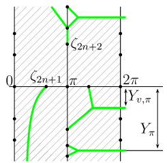
(a) The domain $\mathcal{D}_{\pi}$

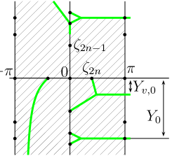
(b) The domain $\mathcal{D}_{0}$

Figure 9. The continuation diagrams

Its boundary consists of the lines bounding $D_{\pi}$ and of the segments of Stokes lines and lines $\{{\rm Re}\,\zeta=C\}$ beginning at the intersection points of Stokes lines. The domain ${\mathcal{D}}_{\pi}$ is simply connected.
Let $\kappa_{\pi}$ be the analytic continuations of $\kappa$ from $S^{p}$ to ${\mathcal{D}}_{\pi}$, i.e., for $\zeta\in{\mathcal{D}}_{\pi}\cap S^{p}$

(7.11) $$\kappa_{\pi}(\zeta)=\kappa(\zeta).$$

Let $\Psi_{+}^{(\pi)}$ be the canonical Bloch solution analytic ${\mathcal{D}}_{\pi}$, normalized at $\pi$ and such that $\kappa_{\pi}$ is its Bloch quasi-momentum. In [9], we have proved

Proposition 7.1 ([9]).

Fix $E=E_{*}\in J$. For sufficiently small $\varepsilon$, there exists $f_{\pi}$, a solution to (5.2), satisfying (5.3) and analytic in the strip $S_{\tilde{Y}}$ that, on ${\mathcal{D}}_{\pi}$, has the standard behavior

(7.12) $$f_{\pi}\sim\exp\left(\frac{i}{\varepsilon}\int_{\pi}^{\zeta}\kappa_{\pi}d\zeta\right)\,\Psi_{+}^{(\pi)}.$$

7.3.2. The solution $f_{0}$

Consider ${\mathcal{D}}_{0}$, the subdomain of the domain $D_{0}=\{|{\rm Im}\,\zeta|<\tilde{Y},\ -\pi<{\rm Re}\,\zeta<\pi\}$ shown in Fig. 9(b). Its boundary consists of the lines bounding $D_{0}$ and of the segments of Stokes lines and lines $\{{\rm Re}\,\zeta=C\}$ beginning at the intersection points of Stokes lines. The domain ${\mathcal{D}}_{0}$ is simply connected.
Let $\kappa_{0}$ be the analytic continuation of $-\kappa$ from $S^{p}$ to ${\mathcal{D}}_{0}$ i.e., for $\zeta\in{\mathcal{D}}_{0}\cap S^{p}$,

(7.13) $$\kappa_{0}(\zeta)=-\kappa(\zeta).$$

Let $\Psi_{+}^{(0)}$ be the canonical Bloch solution analytic ${\mathcal{D}}_{0}$, normalized at $0$ and such that $\kappa_{0}$ is its Bloch quasi-momentum. One has

Proposition 7.2.

Fix $E=E_{*}\in J$. For sufficiently small $\varepsilon$, there exists $f_{0}$, a solution to (5.2), satisfying (5.3) and analytic in the strip $S_{\tilde{Y}}$ that, on ${\mathcal{D}}_{0}$, has the standard behavior

(7.14) $$f_{0}\sim\exp\left(\frac{i}{\varepsilon}\int_{0}^{\zeta}\kappa_{0}d\zeta\right)\,\Psi_{+}^{(0)}.$$

The proof of Proposition 7.2 is similar to that of Proposition 7.1; we omit it.

8. Two consistent bases

In this section, we construct the consistent bases used in the section 5.1.
Fix $\nu\in\{0,\pi\}$. The solution $f_{\nu}^{*}$ is related to $f_{\nu}$ by the transformation (2.10). First, we compute the asymptotics of $f_{\nu}^{*}$. Then, we compute the asymptotic of the Wronskian $w(f_{\nu},f_{\nu}^{*})$. This Wronskian is constant up to a factor of the form $(1+o(1))$. Finally, we correct $f$ so that

1. the Wronskian $w(f_{\nu},f_{\nu}^{*})$ be constant (and, thus, $f_{\nu}$ and $f_{\nu}^{*}$ form a consistent basis),

2. the “new” solutions $f_{\nu}$ and $f_{\nu}^{*}$ have the “old” behavior in the strip $S_{\tilde{Y}}$.

The constructions described here are standard for the adiabatic complex WKB method. The proofs of Lemmas 8.1 and 8.2, and of Theorem 8.1 below essentially repeat the proofs of the analogous statements found in [10] and are therefore omitted.

8.1. Asymptotics of $f_{\nu}^{*}$

To discuss the asymptotic behavior of $f_{\nu}^{*}$, we need some additional material.

8.1.1. Preparation

Define $\mathfrak{z}_{0}=(-\zeta_{2n},\zeta_{2n})\subset{\mathbb{R}}$ and $\mathfrak{z}_{\pi}=(\zeta_{2n+1},2\pi-\zeta_{2n+1})\subset{\mathbb{R}}$. Note that $\mathcal{E}$ maps $\mathfrak{z}_{0}$ into the $n$-th spectral band, and $\mathfrak{z}_{\pi}$ into the $(n+1)$-st spectral band.
Recall that the leading terms of the asymptotics of the solutions having standard asymptotic behavior are fixed up to the choice of $q$, the branch of $\sqrt{k^{\prime}({\mathcal{E}}(\zeta))}$ from the definition of the canonical Bloch solution, see (7.6). Let $q_{\nu}$ be the branch of $q$ from the definition of $\Psi_{+}^{(\nu)}$. Fix it so that

$$q_{\nu}(\zeta)>0\quad\text{for}\quad\zeta\in{\mathfrak{z}}_{\nu}.$$

This choice is possible as, inside any spectral band of the periodic operator, $k_{p}^{\prime}>0$.

8.1.2. The asymptotics

Let ${\mathcal{D}}_{\nu}^{*}$ be the domain symmetric to ${\mathcal{D}}_{\nu}$ with respect to the real line. Note that $\mathfrak{z}_{\nu}\subset\mathcal{D}_{\nu}\cap\mathcal{D}_{\nu}^{*}$. One has

Lemma 8.1.

In $\mathcal{D}_{\nu}^{*}$, the solution $f_{\nu}^{*}$ has the standard behavior

(8.1) $$f_{\nu}^{*}\sim e^{-\frac{i}{\varepsilon}\int_{\nu}^{\zeta}\kappa_{\nu,*}d\zeta}\,\Psi_{-}^{(\nu),*}(x,\zeta).$$

Here, $\kappa_{\nu,*}$ is the branch of the complex momentum analytic in $\mathcal{D}_{\nu}^{*}$ that coincides with $\kappa_{\nu}$ on $\mathfrak{z}_{\nu}$; the function $\Psi_{-}^{(\nu),*}$ is the canonical Bloch solution analytic in $\mathcal{D}_{\nu}^{*}$ that coincides with $\Psi_{-}^{(\nu)}$ (complementary to $\Psi_{+}^{(\nu)}$ from the asymptotics of $f_{\nu}$) on ${\mathfrak{z}}_{\nu}$.

The proof of Lemma 8.1 mimics that of Lemma 6.1 in [10].
Note that $\kappa_{\nu,*}=\kappa_{\nu}^{*}$, and that $\Psi_{-}^{(\nu),*}=(\Psi_{+}^{(\nu)})^{*}$.

8.2. The Wronskian of $f_{\nu}$ and $f_{\nu}^{*}$

The solution $f_{\nu}$ and $f_{\nu}^{*}$ are analytic in the strip $S_{\tilde{Y}}$; so does their Wronskian. As both $f_{\nu}$ and $f_{\nu}^{*}$ satisfy condition (5.3), it is $\varepsilon$-periodic in $\zeta$. One has

Lemma 8.2.

The Wronskian of $f_{\nu}$ and $f_{\nu}^{*}$ admits the asymptotic representation:

(8.2) $$w(f_{\nu},f_{\nu}^{*})=w(\Psi_{+}^{(\nu)},\Psi_{-}^{(\nu)})|_{\zeta=\nu}+g_{\nu},\quad\quad\zeta\in S_{\tilde{Y}}.$$

Here, $g_{\nu}$ is a function analytic in $S_{\tilde{Y}}$ such that, for real $\zeta$ and $E$, ${\rm Re}\,g_{\nu}=0$. Moreover, $g_{\nu}=o(1)$ locally uniformly in any compact of $S_{\tilde{Y}}$ provided that $E$ is in a sufficiently small complex neighborhood of $E_{0}$.

The proof of Lemma 8.2 mimics that of Lemma 6.2 in [10].

Remark 8.1.

Note that $w(\Psi_{+}^{(\nu)},\Psi_{-}^{(\nu)})|_{\zeta=\nu}\neq 0$ as $\mathcal{E}(\nu)\not\in P\cup Q$.

As $g_{\nu}$, the error term in (8.2), may depend on $\zeta$, we redefine the solution $f_{\nu}$ setting

$$f_{\nu}:=f_{\nu}/Q\quad\text{where}\quad Q=\sqrt{1+g/w(\Psi_{+}^{(\nu)},\Psi_{-}^{(\nu)})|_{\zeta=\nu}}.$$

In terms of this new solution $f_{\nu}$, we define the new $f_{\nu}^{*}$. The solutions $(f_{\nu},f_{\nu}^{*})$ form the basis the monodromy matrix of which we study. For these “new” $f_{\nu}$ and $f_{\nu}^{*}$, we have

Theorem 8.1.

The solutions $f_{\nu}$ and $f_{\nu}^{*}$ are analytic in $S_{\tilde{Y}}$, satisfy the condition (5.3), and

(8.3) $$w(f_{\nu},f_{\nu}^{\ast})=w(\Psi_{+}^{(\nu)},\Psi_{-}^{(\nu)})|_{\zeta=\nu}.$$

Moreover, $f_{\nu}$ has the standard behavior, (7.14) or (7.12), in ${\mathcal{D}}_{\nu}$, and $f_{\nu}^{*}$ has the standard behavior (8.1) in $\mathcal{D}_{\nu}^{*}$.

The proof of Theorem 8.1 mimics that of Theorem 6.1 from [10].
Let $\zeta\mapsto\psi_{\pm}(x,{\mathcal{E}}(\zeta))$ be the two branches of the Bloch solution $\zeta\mapsto\psi(x,{\mathcal{E}}(\zeta))$ that are analytic in $\zeta\in S^{p}$ and such that $\kappa$, the branch of the complex momentum defined in the beginning of the section 7.3, is the Bloch quasi-momentum for $\psi_{+}$. By (7.7) and the definitions of the canonical Bloch solutions $\Psi_{\pm}^{\nu}$, one has

(8.4) $$w(\Psi_{+}^{(\nu)},\Psi_{-}^{(\nu)})|_{\zeta=\nu}=s(\nu)k_{p}^{\prime}({\mathcal{E}}(\nu))\,w(\psi_{+},\psi_{-})|_{\zeta=\nu},\quad{\rm where}\quad s(\nu)=\left\{\begin{array}[]{l}1\text{ if }\nu=\pi,\\ -1\text{ if }\nu=0.\end{array}\right.$$

9. Transition matrices

In this section, we compute the asymptotics of the transition matrices $T_{\nu}$ defined by (5.6) for the bases $(f_{\nu},f^{*}_{\nu})$ for $\nu\in\{0,\pi\}$.

9.1. Elementary properties of the transition matrices

One can easily express the coefficients of the transition matrices, see (5.6), via the Wronskians of the basis solutions; formulas (5.6) immediately imply

Lemma 9.1.

One has

(9.1) $$a_{\pi}(\zeta)=\frac{w(f_{\pi}(\cdot,\zeta+2\pi),f_{0}^{*}(\cdot,\zeta))}{w(f_{0}(\cdot,\zeta),f_{0}^{*}(\cdot,\zeta))},\quad b_{\pi}(\zeta)=\frac{w(f_{0}(\cdot,\zeta),f_{\pi}(\cdot,\zeta+2\pi))}{w(f_{0}(\cdot,\zeta),f_{0}^{*}(\cdot,\zeta))}.$$

and

(9.2) $$a_{0}(\zeta)=\frac{w(f_{0}(\cdot,\zeta),f_{\pi}^{*}(\cdot,\zeta))}{w(f_{\pi}(\cdot,\zeta),f_{\pi}^{*}(\cdot,\zeta))},\quad b_{0}(\zeta)=\frac{w(f_{\pi}(\cdot,\zeta),f_{0}(\cdot,\zeta))}{w(f_{\pi}(\cdot,\zeta),f_{\pi}^{*}(\cdot,\zeta))}.$$

For $\nu\in\{0,\pi\}$, by the definition of the standard behavior, the basis $\{f_{\nu},f_{\nu}^{*}\}$ is defined and analytic for $(\zeta,E)\in S_{\tilde{Y}}\times V(\tilde{Y})$ where $V(\tilde{Y})$ is a neighborhood of $E_{*}\in J$; this neighborhood is independent of $\varepsilon$. One has

Lemma 9.2.

Pick $\nu\in\{0,\pi\}$. The matrix $T_{\nu}$ is analytic and $\varepsilon$-periodic in $\zeta\in S_{\tilde{Y}}$ and analytic in $E\in V(\tilde{Y})$. Moreover, $\det T_{\nu}$ is independent of $\zeta$ and does not vanish.

Proof.  As the solutions $f_{\nu}$ and $f_{\nu}^{*}$ are analytic functions of the variables $\zeta$ and $E$, so are the Wronskians in formulae (9.1) and (9.2). Moreover, by (8.3), the Wronskians in the denominators of (9.1) and (9.2) do not vanish. This implies the analyticity of the coefficients of the transition matrices. The periodicity in $\zeta$ follows from the fact that all the solutions satisfy (5.3). Finally, relations (5.6) imply that

(9.3) $$w(f_{\pi}(x,\zeta+2\pi),f_{\pi}^{*}(x,\zeta+2\pi))=\det T_{\pi}\,w(f_{0}(x,\zeta),f_{0}^{*}(x,\zeta)).$$

Now, (8.3) imply that $\det T_{\pi}$ is independent of $\zeta$. Similarly one checks that $\det T_{0}$ is independent of $\zeta$. This completes the proof of Lemma 9.2.∎

9.2. The asymptotics of the transition matrices

We first introduce some notations:

1. For the Fourier coefficients of $a_{\nu}$ and $b_{\nu}$ we use the notations introduced in (5.9), and recall that $p(z)=e^{2\pi|{\rm Im}\,z|}$.

2. Let $Y_{\pi}$, $Y_{v,\pi}$ and $Y_{0}$, $Y_{v,0}$ be the distances marked in Fig. 9(a) and Fig. 9(b) respectively. E.g., $Y_{0}$ is the imaginary part of the point of intersection of the Stokes lines $\overline{``g^{\prime\prime}}$ and $\overline{``h^{\prime\prime}}$ (see Lemma 7.2). Note that, for any $\nu\in\{0,\pi\}$, one has

   (9.4) $$0<Y_{v,\nu}<Y_{\nu}<\tilde{Y}.$$

3. We use the branch $\kappa$ introduced in the beginning of the section 7.3; $\psi_{\pm}$ (resp. $\Omega_{\pm}$) are the branches of $\psi(x,{\mathcal{E}}(\cdot))$ (resp. $\Omega$) such that $\kappa$ is the Bloch quasi-momentum of $\psi_{+}$. When integrating $\kappa$ (resp. integrating $\Omega$ or continuing analytically $\psi$) along a curve, we choose a branch of $\kappa$ (resp. $\Omega$, $\psi$) near the starting point of the curve and then continue it along the curve.

4. Let $\gamma$ be a curve and $g$ be a function continuous on $\gamma$. We denote by $\Delta\arg q|_{\gamma}$ the increment of the argument $q(\zeta)$ along the curve $\gamma$.

The asymptotics of the transition matrices coefficients are described by

Proposition 9.1.

Pick $\nu\in\{0,\pi\}$. Fix $Y$ so that $Y_{v,\nu}<Y<Y_{\nu}$. There exists $V_{\nu}(Y)$, a complex neighborhood of $E_{*}$ independent of $\varepsilon$, such that, for $\varepsilon$ sufficiently small, $j\in\{0,1\}$ and $E\in V_{\nu}(Y)$, one has the uniform asymptotics

(9.5) $$a_{\nu,j}=\exp\left(s\frac{i}{\varepsilon}\int_{\alpha}\kappa d\zeta-j\frac{2\pi(\pi-\nu)i}{\varepsilon}+\int_{\alpha}\Omega_{s}+i\Delta\arg q|_{\alpha}+o(1)\right),\quad\alpha=\alpha_{\nu,j},$$

(9.6) $$b_{\nu,j}=\exp\left(s\frac{i}{\varepsilon}\int_{\beta}\kappa d\zeta-j\frac{2\pi(\pi-\nu)i}{\varepsilon}+\int_{\beta}\Omega_{s}+i\Delta\arg q|_{\beta}+o(1)\right),\quad\beta=\beta_{\nu,j},$$

$$\text{where }\quad s=+1\ \text{if}\quad\nu=\pi,\text{ and }s=-1\ \text{if}\quad\nu=0.$$

In (9.5) and (9.6), one integrates along the curves shown in Fig. 10 chosen such that ${\mathcal{E}}(\zeta)\not\in(P\cup Q)$ along them; for each of the integration curves, $q$ denotes a branch of $\zeta\mapsto\sqrt{k^{\prime}({\mathcal{E}}(\zeta))}$ continuous on this curve.
For $(\zeta,E)\in S(Y)\times V_{\nu}(Y)$, one has the uniform estimates

(9.7) $$a_{\nu,-1}(\zeta)=o(a_{\nu,0}),\quad b_{\nu,-1}(\zeta)=o(b_{\nu,0}),\quad a_{\nu,2}(\zeta)=o(p(\zeta/\varepsilon)a_{\nu,1}),\quad b_{\nu,2}(\zeta)=o(p(\zeta/\varepsilon)b_{\nu,1}).$$

Figure 10. The integrations paths for Theorem 5.1

In the remaining part of the present section, we first explain how Theorem 5.1 is deduced from Proposition 9.1. Then, we turn to the proof of Proposition 9.1. We begin with describing general asymptotic formulae for the Wronskians of two solutions having standard behavior; this material mostly stems from [10]. Then, using these formulae, we compute the Wronskians in the formulae for the transition matrix coefficients (see Lemma 9.1) and, thus, complete the proof of Proposition 9.1. Note that we carry out the analysis only for the asymptotics and the estimates for $a_{0}$ and $b_{0}$. The coefficients $a_{\pi}$ and $b_{\pi}$ are analyzed in a similar way.

9.3. The proof of Theorem 5.1

In section 10, we study the actions $(S_{v,\nu})_{\nu\in\{0,\pi\}}$ and prove

Lemma 9.3.

Pick $E_{*}\in J$. For each $\nu\in\{0,\pi\}$, one has $S_{v,\nu}(E_{*})=2\pi Y_{v,\nu}(E_{*})$.

Lemma 9.3 and the condition (T), see section 1.5, imply that, in Proposition 9.1, we can choose $Y$ so that (1) $2\pi Y>\max_{E\in J}S_{h}(E)$ and (2) $Y_{v,\nu}<Y<Y_{\nu}$ simultaneously for $\nu=0$ and $\nu=\pi$. We then define $V_{*}=V_{0}\cap V_{\pi}$. With this, each of the basis solutions $f_{0}$, $f^{*}_{0}$, $f_{\pi}$ and $f_{\pi}^{*}$ is defined and analytic in the domain (5.5). This and Lemma 9.2 imply the first and the second point of Theorem 5.1.
In section 11, we derive the estimates of the third point of Theorem 5.1 from the asymptotics (9.5) and (9.6).
Finally, the last point of Theorem 5.1 is an immediate consequence of the estimates (9.7). So, Theorem 5.1 is proved.

9.4. General asymptotic formulae

We recall results from section 8 of [10]. Consider equation (7.1) assuming only that $W$ is analytic and that $E$ is fixed, say $E=E_{0}$. Let $h$ and $g$ be two solutions of (7.1) having the standard asymptotic behavior in regular domains $D_{h}$ and $D_{g}$:

(9.8) $$h\sim e^{\frac{i}{\varepsilon}\int_{\zeta_{h}}^{\zeta}\kappa_{h}d\zeta}\,\Psi_{h}(x,\zeta),\quad g\sim e^{\frac{i}{\varepsilon}\int_{\zeta_{g}}^{\zeta}\kappa_{g}d\zeta}\,\Psi_{g}(x,\zeta).$$

Here, $\kappa_{h}$ (resp. $\kappa_{g}$) is a branch of the complex momentum analytic in $D_{h}$ (resp. $D_{g}$), $\Psi_{h}$ (resp. $\Psi_{g}$) is the canonical Bloch solution defined on $D_{h}$ (resp. $D_{g}$) and having the quasi-momentum $\kappa_{h}$ (resp. $\kappa_{g}$), and $\zeta_{h}$ (resp. $\zeta_{g}$) is the normalization point for $h$ (resp. $g$).
As the solutions $h$ and $g$ satisfy the consistency condition, their Wronskian is $\varepsilon$-periodic in $\zeta$. First, following [10], we describe the asymptotics of this Wronskian and of its Fourier coefficients. Then, we develop simple tools to compute some constants coming up in these formulae.

9.4.1. Asymptotics of the Wronskian

Let $d$ be a simply connected domain such that $d\subset D_{h}\cap D_{g}$.
Arcs.  Let $\gamma$ be a curve connecting $\zeta_{g}$ to $\zeta_{h}$ going first from $\zeta_{g}$ to some point in $d$ while in $D_{g}$ and, then, from this point to $\zeta_{h}$ while in $D_{h}$. We call $\gamma$ an arc associated to the triple $(g,h,d)$ and denote it by $\gamma(g,h,d)$.
Two arcs associated to one and the same triple are called equivalent.

Continue $\kappa_{h}$ and $\kappa_{g}$ analytically along $\gamma(g,h,d)$. Then, there exists $m\in{\mathbb{Z}}$ and $\sigma\in\{-1,+1\}$ such that for $\zeta$ close to $\gamma$, one has

(9.9) $$\kappa_{g}(\zeta)=\sigma\kappa_{h}(\zeta)+2\pi m.$$

We call $\sigma=\sigma(g,h,d)$ the signature of $\gamma$, and $m=m(g,h,d)$ the index of $\gamma$. These two integers do not change when we replace the arc $\gamma$ by an equivalent one.
Meeting domains.  A domain $d$ is called a meeting domain if the functions ${\rm Im}\,\kappa_{h}$ and ${\rm Im}\,\kappa_{g}$ do not vanish and are of opposite sign in $d$. One has

Lemma 9.4 ([10]).

Suppose the functions ${\rm Im}\,\kappa_{h}$ and ${\rm Im}\,\kappa_{g}$ do not vanish in $d$. Then, $d$ is a meeting domain if and only if $\sigma(g,h,d)=-1$.

Fourier coefficients.  Let $S(d)$ be the smallest strip of the form $\{C_{1}<{\rm Im}\,\zeta<C_{2}\}$ containing the domain $d$. One has

Proposition 9.2 ([10]).

Fix $E_{0}$. Let $d=d(h,g)$ be a meeting domain for $h$ and $g$, and $m=m(g,h,d)$ be the corresponding index (at energy $E_{0}$). Then, there exists $V_{0}$ a neighborhood of $E_{0}$ such that for $\varepsilon$ sufficiently small, for $E\in V_{0}$ and $\zeta\in S(d)$, the Wronskian of $h$ and $g$ is given by the formulae

(9.10) $$w(h,g)=\tilde{w}_{m}\,e^{\frac{2\pi im}{\varepsilon}(\zeta-\zeta_{h})}(1+o(1)),$$

where

(9.11) $$\tilde{w}_{m}=\left.\left(q_{g}/q_{h}\right)\right|_{\zeta=\zeta_{h}}\,\exp\left(\frac{i}{\varepsilon}\int_{\gamma(g,h,d)}\kappa_{g}d\zeta+\int_{\zeta_{g}}^{\zeta_{h}}\Omega_{g}\right)\,w(\Psi_{+},\Psi_{-})_{|\zeta=\zeta_{g}}.$$

In these formulae:

• $\tilde{w}_{m}$ is independent of $\zeta$;

• we choose the arc $\gamma(g,h,d)$ so that, along it, $\mathcal{E}(\zeta)\not\in P\cup Q$;

• $\zeta\mapsto q_{g}(\zeta)=\sqrt{k^{\prime}(\mathcal{E}(\zeta))}$ and $\zeta\mapsto\Omega_{g}(\zeta)=\Omega_{g}(\mathcal{E}(\zeta))$ are the analytic continuations of the function and the 1-form from the definition of $\Psi_{g}$ along $\gamma(g,h,d)$.

• $\Psi_{+}=\Psi_{h}$, and $\Psi_{-}$ is the canonical Bloch solution “complementary” to $\Psi_{+}$.

Fix $K$, a compact subset of $S(d)$. Then, there exists $V^{K}_{0}$ a neighborhood of $E_{0}$ in $V_{0}$ such that the asymptotics (9.10) is uniform in $K\times V^{K}_{0}$.

The factor $\tilde{w}_{m}$ is the leading term of the asymptotics of the $m$-th Fourier coefficient of $w(h,g)$.

9.4.2. Closed curves and the index $m$

In practice, it is not too difficult to compute the index $m$. However, as one needs to control several Fourier coefficients of each Wronskian, the computations become lengthy. Fortunately, there is an effective way to compare the indexes of two (non-equivalent) arcs. To this end, we define the index of a closed curve.

Closed curves. Let $c$ be an oriented closed curve containing no branch points of the complex momentum. Pick $\zeta_{0}\in c$. In $V_{0}$, a regular neighborhood of $\zeta_{0}$, fix $\kappa$, an analytic branch of the complex momentum. We call the triple $(c,\zeta_{0},\kappa)$ a loop.
We shall consider $c$ as disjoint at $\zeta_{0}$ and speak about its beginning and its end. Continue $\kappa$ analytically along $c$. This yields a new branch of the complex momentum in $V_{0}$. Denote it by $\kappa|_{c}$. Hence, there exists $\sigma\in\{-1,+1\}$ and $m\in{\mathbb{Z}}$ such that, for $\zeta\in V_{0}$

(9.12) $$\kappa|_{c}(\zeta)=\sigma\kappa(\zeta)+2\pi m.$$

The numbers $\sigma=\sigma(c,\zeta_{0},\kappa)$ and $m=m(c,\zeta_{0},\kappa)$ are called the signature and the index of the loop $(c,\zeta_{0},\kappa)$.
Consider two loops $(c_{1},\zeta_{1},\kappa_{1})$ and $(c_{2},\zeta_{2},\kappa_{2})$. Assume that one can continuously deform $c_{1}$ into $c_{2}$ without intersecting any branching point. Assume moreover that, in result of the same deformation, $\zeta_{1}$ becomes $\zeta_{2}$. This deformation defines an analytic continuation of $\kappa_{1}$ to a neighborhood of $\zeta_{2}$. If this analytic continuation coincides with $\kappa_{2}$, we say that the loops are equivalent. The indexes $m$ and $\sigma$ calculated for equivalent loops coincide.

Let us explain how to compute the indexes $m$ and $\sigma$. Let $G$ be the pre-image with respect to $\mathcal{E}$ of the set of the spectral gaps of the periodic operator (0.2). Note that

• on any connected component of $G$, the value of the real part of the complex momentum is constant and belongs to $\{\pi l;\ l\in{\mathbb{Z}}\}$;

• locally, outside $\{\zeta;\ W^{\prime}(\zeta)=0\}$, all the connected components of $G$ are analytic curves.

Now, we can formulate

Lemma 9.5.

Assume that $c$ does not start at a point of $G$. Assume moreover that $c$ intersects $G$ exactly $N$ times ($N<\infty$) and that, at the intersection points, $W^{\prime}\neq 0$. Let $r_{1}$, $r_{2}$, …, $r_{N}$ be the values that ${\rm Re}\,\kappa$ takes consecutively at these intersection points as $\zeta$ moves along $c$ (from the beginning to the end). Then,

(9.13) $$\sigma(c,\zeta_{0},\kappa)=(-1)^{N},\quad\text{ and }\quad m(c,\zeta_{0},\kappa)=\frac{1}{\pi}\,\left(r_{N}-r_{N-1}+r_{N-2}-\dots+(-1)^{N-1}r_{1}\right).$$

The proof of Lemma 9.5 mimics the proof of Lemma 8.2 in [10] which describes the index of a $2\pi$-periodic curve.

Comparing the indexes of arcs. Let $d$ and $\tilde{d}$ be two (distinct) meeting domains for the solutions $h$ and $g$, and let $\gamma$ and $\tilde{\gamma}$ be the corresponding arcs. One can write

(9.14) $$\tilde{\gamma}=c+\gamma,$$

where $c$ is a closed regular curve; its orientation is induced by those of $\gamma$ and $\tilde{\gamma}$.
As $\sigma(g,h,\tilde{d})=\sigma(g,h,d)=-1$, one has $\sigma(c,\zeta_{g},\kappa_{g})=1$. As an immediate consequence of the definitions, we also get

(9.15) $$m(g,\tilde{h},\tilde{d})=m(c,\zeta_{g},\kappa_{g})+m(g,h,d).$$

This formula and Lemma 9.5 give an effective way to compute the indexes of arcs.

9.5. The asymptotics of the coefficient $b_{0}$

The coefficient $b_{0}$ of the matrix $T_{0}$ is given in (9.2). As $w(f_{\pi},f_{\pi}^{*})$ is given by formula (8.3), we have only to compute $w(f_{\pi}(\cdot,\zeta),f_{0}(\cdot,\zeta))$. One applies the constructions of section 9.4 with

$$h(x,\zeta)=f_{\pi}(x,\zeta),\quad g(x,\zeta)=f_{0}(x,\zeta),\quad D_{h}=\mathcal{D}_{\pi},\quad D_{g}=\mathcal{D}_{0};$$

(9.16) $$\zeta_{h}=\pi,\quad\zeta_{g}=0;$$

(9.17) $$\kappa_{h}(\zeta)=\kappa(\zeta)\text{ for }\zeta\sim\pi,\quad\text{and}\quad\kappa_{g}(\zeta)=-\kappa(\zeta)\text{ for }\zeta\sim 0.$$

In (9.17), $\kappa$ is the branch of the complex momentum defined in (7.10).
Let $Y_{0}$ and $Y_{v,0}$ be the distances marked in Fig. 9(b). They satisfy (9.4).

9.5.1. The asymptotics in the strip $\{-Y_{v,0}<{\rm Im}\,\zeta<Y_{0}\}$

Let us describe $d_{0}$, the meeting domain, and $\gamma(f_{0},f_{\pi},d_{0})$, the arc used to compute $w(f_{\pi},f_{0})$ in the strip

$$S_{0}=\{\zeta\in{\mathbb{C}};\ -Y_{v,0}<{\rm Im}\,\zeta<Y_{0}\}.$$

The meeting domain $d_{0}$. It is the subdomain of the strip $S_{0}$ between the lines $\gamma_{1}$ and $\gamma_{2}$ defined by

• the line $\gamma_{1}$ consists of the following lines: the Stokes line $\overline{\text{``e''}}$ symmetric to the Stokes line “e” with respect to the real line, the segment $[0,\zeta_{2n}]$ of the real line, the segment $[0,\zeta_{2n-2}]$ of the imaginary axis and the Stokes line “g” (see Fig. 8);

• the line $\gamma_{2}$ consists of the following lines: the Stokes line $\overline{\text{``a''}}$ symmetric to the Stokes line “a” with respect to the real line, the segment $[\zeta_{2n+1},\pi]$ of the real line, the segment $[\pi,\zeta_{2n+3}]$ of the line ${\rm Re}\,\zeta=\pi$ and the Stokes line “c” (see Fig. 8).

The Stokes lines mentioned here are described by Lemmas 7.1 and 7.2. In particular, these lemmas imply that $\gamma_{1}\cap\gamma_{2}=\emptyset$.
Note that $d_{0}$ does not intersect $Z$, the pre-image of the set of the bands of the periodic operator (0.2) with respect to the mapping $\mathcal{E}$. So, in $d_{0}$, one has ${\rm Im}\,\kappa\neq 0$.

The arc $\gamma(g,h,d_{0})$. It is the curve $\beta_{0,0}$ shown in Fig. 10; it stays in $d_{0}$ and connects $\zeta_{g}=0$ to $\zeta_{h}=\pi$.
Index $m$. In view of (9.17), in $d_{0}$, one has $\kappa_{h}=-\kappa_{g}$. This implies that $m(g,h,d_{0})=0$.
The result.  Proposition 9.2, formulae (9.2) and (8.3) imply that, for $\zeta\in S_{0}$,

(9.18) $$b_{0}=\tilde{b}_{0}(1+o(1)),\quad\tilde{b}_{0}=\exp\left(-\frac{i}{\varepsilon}\int_{\beta}\kappa d\zeta+\int_{\beta}\Omega_{-}+i\Delta\arg q|_{\beta}\right)\text{ where }\beta=\beta_{0,0},$$

and, as $q$, one can take any branch of the function $\zeta\mapsto\sqrt{k^{\prime}({\mathcal{E}}(\zeta))}$ continuous on $\beta$.
When deriving the formula for $\tilde{b}_{0}$, we have used the facts that

• $\Omega_{g}$ is the branch of $\Omega_{-}$ corresponding to the branch $\kappa$ chosen above;

• $(q_{g}/q_{h})(\zeta_{h})=e^{i\Delta\arg q_{g}|_{\beta}}$ as, at $\zeta_{h}$, $q_{h}$ is real and $|q_{g}/q_{h}|=1$;

• the quantity $\Delta\arg q_{g}|_{\beta}$ does not depend on the branch of $q_{g}$ as long as it is continuous on $\beta$.

9.5.2. The asymptotics in the strip $\{-Y_{0}<{\rm Im}\,\zeta<-Y_{v,0}\}$

Let us describe $d_{1}$, the meeting domain, and $\gamma(f_{\pi},f_{0},d_{1})$, the arc used to compute $w(f_{\pi},f_{0})$ in this strip

$$S_{1}=\{\zeta\in{\mathbb{C}};\ -Y_{0}<{\rm Im}\,\zeta<-Y_{v,0}\}.$$

The meeting domain $d_{1}$. Let $d_{1}$ be the subdomain of the strip $S_{1}$ located between the Stokes line $\overline{\text{``a''}}$ (symmetric to “a” with respect to the real line) and $\gamma_{3}$, the curve which consists of the following lines:

• the Stokes line $\overline{\text{``f''}}$ symmetric to the Stokes line “f” with respect to the real line, the segment $[\overline{\zeta_{2n-1}},\overline{\zeta_{2n-2}}]$ of the imaginary axis, and the Stokes line $\overline{\text{``g''}}$ symmetric to the Stokes line “g” with respect to the real line.

The domain $d_{1}$ is a meeting domain in view of

Lemma 9.6.

In $d_{1}$, one has ${\rm Im}\,\kappa_{\pi}=-{\rm Im}\,\kappa_{0}>0$.

Proof.  The sign of ${\rm Im}\,\kappa$ remains the same in any regular domain $D$ such that $D\cap Z=\emptyset$. Moreover, the sign of ${\rm Im}\,\kappa$ flips as $\zeta$ intersects (transversally) a connected component of $Z$ at a point where $W^{\prime}$ does not vanish.
By (7.10) and (7.11), one has ${\rm Im}\,\kappa_{\pi}={\rm Im}\,\kappa={\rm Im}\,\kappa_{p}>0$ in ${\mathcal{D}}_{\pi}\cap\Pi$. As one goes from $\Pi$ to $d_{1}$ in ${\mathcal{D}}_{\pi}$ without intersecting $Z$, we get ${\rm Im}\,\kappa_{\pi}(\zeta)>0$ for $\zeta\in d_{1}$. Similarly, by (7.10) and (7.13), one has ${\rm Im}\,\kappa_{0}=-{\rm Im}\,\kappa_{p}<0$ in ${\mathcal{D}}_{0}\cap\Pi$. Furthermore, to go from $\Pi$ to $d_{1}$ staying in ${\mathcal{D}}_{0}$, one has to intersect two connected components of $Z$, namely, the segment $[-\zeta_{2n},\zeta_{2n}]$ of the real line and the segment $[-\zeta_{2n-1},\zeta_{2n-1}]$ of the imaginary axis. Hence, ${\rm Im}\,\kappa_{0}(\zeta)<0$ for $\zeta\in d_{1}$. This completes the proof of Lemma 9.6. ∎

The arc $\gamma(g,h,d_{1})$. It is the curve $\beta_{0,1}$ shown in Fig. 10; it connects $\zeta_{g}=0$ to $\zeta_{h}=\pi$.

Index $m$. One has

$$\gamma(g,h,d_{1})=c_{0}+\gamma(g,h,d_{0}),$$

where $c_{0}$ is the closed curve shown in Fig. 11. By (9.15), we get

$$m(g,h,d_{1})=m(c_{0},0,\kappa_{g})+m(g,h,d_{0})=m(c_{0},0,\kappa_{g}).$$

Figure 11. The curve $c_{0}$

So, the index $m(g,h,d_{1})$ is equal to the index of the loop $(c_{0},0,\kappa_{g})$. Recall that the indexes of equivalent loops coincide. To compute the index, we pick a point $\zeta_{0}\in c_{0}$ as shown in Fig. 11 and we replace the loop $(c_{0},0,\kappa_{g})$ by the equivalent loop defined by the same curve $c_{0}$ and the point $\zeta_{0}$. The branch of the complex momentum fixed for this new loop is the analytic continuation of the old branch along $c_{0}$ from $0$ to $\zeta_{0}$ in the clockwise direction. For this new branch, we keep the old notation $\kappa_{g}$.
In view of Lemma 9.5, it is sufficient to compute $\kappa_{g}$ at the intersections of $c_{0}$ and $G$. The set $G$ is $2\pi$-periodic and symmetric with respect to the real line and to the imaginary axis. The connected components of $G$ located in the $\{0\leq{\rm Im}\,\zeta,\ 0\leq{\rm Re}\,\zeta\leq\pi\}$ are described in section 7.2.1, part 2.
In Fig. 11, the curve $c_{0}$ intersects two connected components of $G$, the segment $[\overline{\zeta_{2n-1}},\overline{\zeta_{2n-2}}]$ of the imaginary axis and the segment $[\zeta_{2n},\zeta_{2n+1}]$ of the real line. So, Lemma 9.5 implies that

(9.19) $$m(c_{0},0,\kappa_{g})=m(c_{0},\zeta_{0},\kappa_{g})=\frac{1}{\pi}\left({\rm Re}\,\kappa_{g}(\overline{\zeta_{2n-1}})-{\rm Re}\,\kappa_{g}(\zeta_{2n})\right),$$

as ${\rm Re}\,\kappa$ stays constant on any connected component of $G$. As $\kappa_{g}$ is defined by the formulae (9.17) and (7.10), one has

(9.20) $$\kappa_{g}(\zeta_{2n})=-\kappa(\zeta_{2n})=-(\kappa_{p}(\zeta_{2n})-\pi n)=-(\pi n-\pi n)=0.$$

Along the interval $[-\zeta_{2n},\zeta_{2n}]$, one has $\kappa_{g}(\zeta)=-\kappa(\zeta)\in{\mathbb{R}}$; hence,

$$\kappa_{g}(\overline{\zeta_{2n-1}})=-\overline{\kappa(\zeta_{2n-1})}=-\overline{(\kappa_{p}(\zeta_{2n-1})-\pi n)}=-(\pi(n-1)-\pi n)=\pi.$$

Substituting this and (9.20) into (9.19), we finally get

$$m(g,h,d_{1})=m(c_{0},0,\kappa_{g})=1.$$

The result.  Proposition 9.2, formulae (9.2) and (8.3) imply that, for $\zeta\in S_{1}$,

(9.21) $$b_{0}=\tilde{b}_{1}e^{\frac{2\pi i\zeta}{\varepsilon}}(1+o(1)),\quad\tilde{b}_{1}=\exp\left(-\frac{i}{\varepsilon}\int_{\beta}\kappa d\zeta-\frac{2\pi^{2}i}{\varepsilon}+\int_{\beta}\Omega_{-}+i\Delta\arg q|_{\beta}\right)\text{ where }\beta=\beta_{0,1}.$$

Completing the analysis.  The coefficient $b_{0}$ being $\varepsilon$-periodic, we write its Fourier series

(9.22) $$b_{0}(\zeta)=\sum_{l=-\infty}^{\infty}b_{0,l}\,e^{2\pi\,l\,\zeta/\varepsilon}\quad\text{where}\quad b_{0,l}=\frac{1}{\varepsilon}\int_{\tilde{\zeta}}^{\tilde{\zeta}+2\pi}b_{0}(\zeta)e^{-2\pi\,l\,\zeta/\varepsilon}d\zeta\text{ for }l\in{\mathbb{Z}},$$

As $b_{0}$ is analytic in the strip $\{|{\rm Im}\,\zeta|<Y_{0}\}$, $\tilde{\zeta}$ can be taken arbitrarily in the strip $\{|{\rm Im}\,\zeta|<Y_{0}\}$. The asymptotics and the estimates for $b_{0}$ in Proposition 9.1 are obtained by analyzing its Fourier coefficients. To estimate the Fourier coefficients with non-positive index, one uses (9.18) and (9.22) with $\tilde{\zeta}\in S_{0}$. To study the Fourier coefficients with positive index, one uses (9.21) and (9.22) with $\tilde{\zeta}\in S_{1}$. We omit the elementary details and note only that $\tilde{b}_{0}$ in (9.18) is the leading term of the asymptotics of $b_{0,0}$, and that $\tilde{b}_{1}$ in (9.21) is the leading term for $b_{0,1}$.

9.6. The asymptotics of the coefficient $a_{0}$

By (9.2), it suffices to compute the Wronskian $w(f_{0}(\cdot,\zeta),f_{\pi}^{*}(\cdot,\zeta))$. The computations of the coefficient $a_{0}$ follow the same scheme as the ones of $b_{0}$. So, we only outline them. Now,

(9.23) $$h=f_{\pi}^{*},\quad g=f_{0};\quad\quad D_{h}=\mathcal{D}_{\pi}^{*},\quad D_{g}=\mathcal{D}_{0};$$

(9.24) $$\zeta_{h}=\pi,\quad\zeta_{g}=0;$$

(9.25) $$\kappa_{h}(\zeta)=-\overline{\kappa}(\bar{\zeta})\text{ for }\zeta\sim\pi,\quad\text{and}\quad\kappa_{g}(\zeta)=-\kappa(\zeta)\text{ for }\zeta\sim 0.$$

Recall that the complex momentum is real on $[\zeta_{2n+1},2\pi-\zeta_{2n+1}]$. This imply that

(9.26) $$\kappa_{h}(\zeta)=-\kappa(\zeta)\text{ for }\zeta\sim\pi.$$

9.6.1. The asymptotics in the strip $S_{0}$

In this case, the meeting domain $\tilde{d}_{0}$ is the subdomain of the strip $S_{0}$ located between the lines the lines $\gamma_{1}$ and $\overline{\gamma_{2}}$ symmetric to $\gamma_{2}$ with respect to the real line (see section 9.5.1). These two lines do not intersect.
The arc $\gamma(g,h,\tilde{d}_{0})$ is the curve $\alpha_{0,0}$ shown in Fig. 10. One has $m(g,h,\tilde{d}_{0})=0$.
The asymptotics of $a_{0}$ for $\zeta\in S_{0}$ is described by

(9.27) $$a_{0}=\tilde{a}_{0}(1+o(1)),\quad\tilde{a}_{0}=\exp\left(-\frac{i}{\varepsilon}\int_{\alpha}\kappa d\zeta+\int_{\alpha}\Omega_{-}+i\Delta\arg q|_{\alpha}\right)\text{ where }\alpha=\alpha_{0,0}.$$

9.6.2. The asymptotics in the strip $S_{1}$

Now, the meeting domain $\tilde{d}_{1}$ is the subdomain of the strip $S_{1}$ located between the line $\gamma_{3}$ (see section 9.5.2) and the line $\overline{\gamma_{2}}$.
The arc $\gamma(g,h,\tilde{d}_{1})$ is the curve $\alpha_{0,1}$ shown in Fig. 10. One has

$$\gamma(g,h,\tilde{d}_{1})=c_{0}+\gamma(g,h,\tilde{d}_{0}),$$

where $c_{0}$ is the closed curve shown in Fig. 11. The computation done for $b_{0}$ in $S_{1}$ yields

$$m(g,h,\tilde{d}_{1})=m(c_{0},0,\kappa_{g})=1.$$

In result, for $\zeta\in S_{1}$, we get the asymptotic formula

(9.28) $$a_{0}=\tilde{a}_{1}e^{\frac{2\pi i\zeta}{\varepsilon}}(1+o(1)),\quad\tilde{a}_{1}=\exp\left(-\frac{i}{\varepsilon}\int_{\alpha}\kappa d\zeta-\frac{2\pi^{2}i}{\varepsilon}+\int_{\alpha}\Omega_{-}+i\Delta\arg q|_{\alpha}\right)\text{ where }\alpha=\alpha_{0,1}.$$

The asymptotics (9.27) and (9.28) imply the formulae and the estimates for $a_{0}$ in Proposition 9.1.

10. Phase integrals, tunneling coefficients and the iso-energy surface

In this section, we first check the statements found in section 1.3.3. We also prove Lemma 9.3 giving a geometric interpretation of the vertical tunneling coefficients.
Then, we analyze the geometry of the iso-energy curves $\Gamma$ and $\Gamma_{\mathbb{R}}$ (see (0.4) and (0.3)) and justify the interpretation of the phase integrals and tunneling coefficients in terms of these curves.

10.1. The complex momentum on the integration contours

The phase integrals and the tunneling coefficients were defined as contour integrals of the complex momentum along the curves shown in Fig. 3 and 4. We have claimed that, on each of these curves, one can fix a continuous branch of the complex momentum, which we justify in

Lemma 10.1.

Let $\gamma$ be one of the curves $\tilde{\gamma}_{0}$, $\tilde{\gamma}_{\pi}$, $\tilde{\gamma}_{h,0}$, $\tilde{\gamma}_{h,\pi}$, $\tilde{\gamma}_{v,0}$ and $\tilde{\gamma}_{v,\pi}$. Any branch of the complex momentum, analytic in a neighborhood of a point of $\gamma$, can be analytically continued to a single valued function on $\gamma$.

Proof.  The curve $\gamma$ goes exactly around two branch points of the complex momentum. They are of square root type (see section 7.1.1). So, it suffices to check that, at the branch points, the values of the complex momentum coincide. For the curve $\tilde{\gamma}_{h,\pi}$, this follows from the facts that ${\mathcal{E}}$ (defined in (7.8)) bijectively maps the interval $[\zeta_{2n},\zeta_{2n+1}]$ onto the $n$-th spectral gap of the periodic operator, and that the values of a branch of the Bloch quasi-momentum coincide at the ends of a gap. For $\tilde{\gamma}_{\pi}$, this holds as ${\mathcal{E}}$ maps the interval $(\zeta_{2n+1},2\pi-\zeta_{2n+1})$ into the $n$-th spectral band so that both ends are mapped on $E_{2n+1}$. For $\tilde{\gamma}_{v,\pi}$, it holds as ${\mathcal{E}}$ maps the segment $(\zeta_{2n+2},2\pi-\zeta_{2n+2})$ into the $(n+1)$-st spectral band so that both its ends are mapped on $E_{2n+2}$. The analysis of the other curves is done in the same way. ∎

10.2. Independence of the tunneling coefficients and phase integrals on the branch of the complex momentum in their definitions

The independence follows from the observations:

• only the signs of the integrals defining the phase integrals and the tunneling coefficients depend on the choice of the branches of the complex momentum being integrated;

• the branches of the complex momentum being chosen, each of the phase integrals and each of the tunneling action is real and non-zero.

Let us check the first observation. Let $\gamma$ be one of the curves $\tilde{\gamma}_{0}$, $\tilde{\gamma}_{\pi}$, $\tilde{\gamma}_{h,0}$, $\tilde{\gamma}_{h,\pi}$, $\tilde{\gamma}_{v,0}$ and $\tilde{\gamma}_{v,\pi}$. Let $\kappa$ be a branch of the complex momentum continuous on $\gamma$. The formula (7.5) describes all the other branches continuous on $\gamma$. As $\gamma$ is closed, this shows that only the sign of the integral $\oint_{\gamma}\kappa d\zeta$ depends on the choice of the branch $\kappa$.
Recall that $\kappa_{p}$ is analytic in the strip $S^{p}$ (see section 7.3). To prove the second observation, we fix a branch of the complex momentum on each of the integration contours. For $\gamma_{\nu}$ and $\gamma_{h,\nu}$, we fix this branch so that $\kappa=\kappa_{p}-\pi n$ on the parts of the contours in ${\mathbb{C}}_{+}$; for $\gamma_{v,\nu}$, we choose $\kappa=\kappa_{p}-\pi n$ on the parts of the contours in ${\mathbb{C}}_{+}\cap\{\nu<{\rm Re}\,\zeta\}$. We orient the contours $\tilde{\gamma}_{\pi}$, $\tilde{\gamma}_{h,\pi}$ and $\tilde{\gamma}_{v,\pi}$ clockwise, and we orient the contours $\tilde{\gamma}_{0}$, $\tilde{\gamma}_{h,0}$ and $\tilde{\gamma}_{v,0}$ anticlockwise. Then, the second observation follows from

Lemma 10.2.

For $E\in J$, for the above definitions of the integration contours and of the branches of the complex momentum defined on them, each of the functions $\Phi_{\nu}$, $S_{h,\nu}$ and $S_{v,\nu}$ is positive.

Proof.  Begin with $\Phi_{\pi}$. As $\zeta_{2n+1}$ is a square root branch point of $\kappa$, and, as $\kappa(\zeta_{2n+1})=0$, we get

$$\Phi_{\pi}(E)=\int_{\zeta_{2n+1}}^{2\pi-\zeta_{2n+1}}\kappa(\zeta+i0)\,d\zeta,$$

where one integrates along ${\mathbb{R}}$. As ${\mathcal{E}}(\zeta)$ is even, one proves that

(10.1) $$\Phi_{\pi}(E)=2\int_{\zeta_{2n+1}}^{\pi}\kappa(\zeta+i0)\,d\zeta=2\int_{\zeta_{2n+1}}^{\pi}(\kappa_{p}(\zeta)-\pi n)\,d\zeta.$$

Inside the integration interval, one has ${\rm Im}\,\kappa_{p}=0$, and $\pi n<{\rm Re}\,\kappa_{p}<\pi(n+1)$. This implies the positivity of $\Phi_{\pi}$.
Arguing as above, for $S_{h,\pi}$, we get

(10.2) $$S_{h,\pi}(E)=-i\int_{\zeta_{2n}}^{\zeta_{2n+1}}(\kappa_{p}(\zeta)-\pi n)\,d\zeta,$$

where one integrates along ${\mathbb{R}}$. Inside the integration interval, one has ${\rm Re}\,\kappa_{p}=\pi n$ and ${\rm Im}\,\kappa_{p}>0$ so that $S_{h,\pi}>0$.
For $S_{v,\pi}$, one obtains

(10.3) $$S_{v,\pi}(E)=-2i\int_{\zeta_{2n+2}}^{\pi}(\kappa_{p}(\zeta)-\pi(n+1))\,d\zeta,$$

where one integrates along $\pi+i{\mathbb{R}}$. Inside the integration interval, $\pi n<{\rm Re}\,\kappa_{p}<\pi(n+1)$ and ${\rm Im}\,\kappa_{p}=0$ which implies $S_{v,\pi}>0$.
Arguing similarly, one proves the positivity of $\Phi_{0}$, $S_{v,0}$ and $S_{h,0}$. We omit further details. ∎

10.3. Proof of the inequalities (1.4)

One has

$$\Phi_{\pi}(E)=2\int_{\zeta_{2n+1}}^{\pi}(\kappa_{p}(\zeta)-\pi n)\,d\zeta\quad\text{and}\quad\Phi_{0}(E)=-2\int_{0}^{\zeta_{2n}}(\kappa_{p}(\zeta)-\pi n)\,d\zeta.$$

The first equality was established when proving Lemma 10.2. The second is proved similarly. In view of (7.9), we get

$$\Phi_{\pi}^{\prime}(E)=2\int_{\zeta_{2n+1}}^{\pi}k_{p}^{\prime}(E-\alpha\cos\zeta)\,d\zeta\quad\text{and}\quad\Phi_{0}^{\prime}(E)=-2\int_{0}^{\zeta_{2n}}k_{p}^{\prime}(E-\alpha\cos\zeta)\,d\zeta,$$

where $k_{p}$ is the main branch of the Bloch quasi-momentum described in section 6.1.2. As, inside any spectral band of the periodic operator $H_{0}$, the derivative $k^{\prime}_{p}$ is positive, this proves (1.4).

10.4. Proof of (1.9)

We can choose the oriented contours $\tilde{\gamma}_{h,0}$ and $\tilde{\gamma}_{h,\pi}$ so that one be the symmetric of the other with respect to the origin. As ${\mathcal{E}}(\zeta)$ is even, for $\zeta\in\gamma_{h,\pi}$, one has $\kappa(-\zeta)=\kappa(\zeta)$. These two remarks imply relations (1.9).

10.5. Proof of Lemma 9.3

We shall prove the statement of Lemma 9.3 for $\nu=\pi$. For $\nu=0$ the argument is similar. As $S_{v,\pi}(E_{*})\in{\mathbb{R}}$, (10.3) implies that

(10.4) $$S_{v,\pi}(E_{*})={\rm Re}\,S_{v,\pi}(E_{*})=2{\rm Im}\,\int_{\zeta_{2n+2}}^{\pi}(\kappa_{p}(\zeta)-\pi(n+1))\,d\zeta.$$

Let us deform the integration contour in the right hand side so that it go successively

• from $\zeta_{2n+2}$ along the Stokes line “b” to $\zeta_{ba}$, the point of intersection of the Stokes lines “b” and “a” (see Fig. 8),

• from $\zeta_{ba}$ along the Stokes line “a” to $\zeta_{2n+1}$,

• from $\zeta_{2n+1}$ to $\pi$ along the interval $[\zeta_{2n+1},\pi]$ which also is a Stokes line.

As $\kappa_{p}(\zeta_{2n+1})=\pi n$ and $\kappa_{p}(\zeta_{2n+2})=\pi(n+1)$, the definitions of the Stokes lines then imply that

$$S_{v,\pi}(E_{*}) =2{\rm Im}\,\int_{\zeta_{2n+2},{\rm\ along\ ``b^{\prime\prime}}}^{\zeta_{ba}}(\kappa_{p}(\zeta)-\pi(n+1))\,d\zeta+2{\rm Im}\,\int_{\zeta_{ba},{\rm\ along\ ``a^{\prime\prime}}}^{\zeta_{2n+1}}(\kappa_{p}(\zeta)-\pi(n+1))\,d\zeta$$

$$+2{\rm Im}\,\int_{\zeta_{2n+1},{\rm\ along\ }{\mathbb{R}}}^{\pi}(\kappa_{p}(\zeta)-\pi(n+1))\,d\zeta=0+2\pi{\rm Im}\,\zeta_{ba}+0=2\pi{\rm Im}\,\zeta_{ba}.$$

As the set of the Stokes lines is symmetric with respect to both the real line and the line $\pi+i{\mathbb{R}}$, the definition of $Y_{v,\pi}$ implies that ${\rm Im}\,\zeta_{ba}=Y_{v,\pi}(E_{*})$. This and the result of the last computation imply that $S_{v,\pi}(E_{*})=2\pi Y_{v,\pi}(E_{*})$. The proof of Lemma 9.3 is complete.

10.6. The iso-energy curve

The iso-energy curve $\Gamma$ is defined by (0.4). A point $(\zeta,\kappa)\in{\mathbb{C}}^{2}$ belongs to $\Gamma$ if and only if $\kappa$ is one of the values of the complex momentum at the point $\zeta$.
We now discuss the iso-energy curve under the assumptions (H), (O) and (TIBM).

10.6.1. The real branches

Consider the real iso-energy curve $\Gamma_{\mathbb{R}}$ defined by (0.3). Its connected components are the real branches of the iso-energy curve. One has

Lemma 10.3.

The real iso-energy curve is $2\pi$-periodic in both the $\kappa$- and $\zeta$-directions; it is symmetric with respect to each of the lines $\{\kappa=\pi n\}$ and $\{\zeta=\pi m\}$ for $m,n\in{\mathbb{Z}}$.
Any periodicity cell contains exactly two real branches of $\Gamma$. Each of them is homeomorphic to a circle.
There exists $\gamma_{0}$ and $\gamma_{\pi}$, two disjoint connected components of $\Gamma_{\mathbb{R}}$ such that the convex hull of $\gamma_{0}$ contains the point $(0,\pi n)$, and the convex hull of $\gamma_{\pi}$ contains the point $(\pi,\pi n)$.
The curves $\gamma_{0}$ and $\gamma_{\pi}$ are disjoint and are inside the strip $\{\pi(n-1)<\kappa<\pi(n+1)\}$.
Any other real branch of $\Gamma$ can be obtained either from $\gamma_{0}$ or $\gamma_{\pi}$ by $2\pi$-translations in $\kappa$- or/and in $\zeta$-directions.

Proof.  The analysis of $\Gamma_{\mathbb{R}}$ is quite standard. A detailed example can be found in [10]. So, we only outline the proof of Lemma 10.3. The periodicity and the symmetries of $\Gamma_{\mathbb{R}}$ in $\zeta$ follows from the symmetry and periodicity of the cosine and from formula (7.5).
Describe two real branches of $\Gamma$. Recall that one has $\kappa_{p}([\zeta_{2n+1},\pi])\subset[\pi n,\pi(n+1)[$, $\kappa_{p}([0,\zeta_{2n}])\subset]\pi(n-1),\pi n]$ and $\kappa_{p}([\zeta_{2n},\zeta_{2n+1}])\subset\pi n+i{\mathbb{R}}_{+}$. On the first two intervals, $\kappa_{p}$ is monotonously increasing; on the last interval, the imaginary part of $\kappa_{p}$ has only one maximum; this maximum is non degenerate. The graphs of $\kappa_{p}$ on each of the intervals $[0,\zeta_{2n}]$ and $[\zeta_{2n+1},\pi]$ belong to $\Gamma_{\mathbb{R}}$. The real branch $\gamma_{0}$ is obtained from the graph on $[0,\zeta_{2n}]$ by the reflections with respect to the lines $\{\kappa=\pi n\}$ and $\{\zeta=0\}$. The real branch $\gamma_{\pi}$ is obtained from the graph on $[\zeta_{2n+1},\pi]$ by the reflections with respect to the lines $\{\kappa=\pi n\}$ and $\{\zeta=\pi\}$.
We omit further elementary details of the proof. ∎

10.6.2. Complex loops

We prove

Lemma 10.4.

The closed curve $\tilde{\gamma}_{0}$ (resp. $\tilde{\gamma}_{\pi}$, $\tilde{\gamma}_{h,0}$, $\tilde{\gamma}_{h,\pi}$, $\tilde{\gamma}_{v,0}$ and $\tilde{\gamma}_{v,\pi}$) (see figures 3 and 4) is the projection on the $\zeta$-plane of a loop $\gamma_{0}$ (resp. $\gamma_{\pi}$, $\gamma_{h,0}$, $\gamma_{h,\pi}$, $\gamma_{v,0}$ and $\gamma_{v,\pi}$) that is located on $\Gamma$. These loops satisfy:

• the loop $\gamma_{h,\pi}$ connects the real branches $\gamma_{\pi}$ and $\gamma_{0}$;

• the loop $\gamma_{h,0}$ connects the real branches $\gamma_{0}$ and $\gamma_{\pi}-(2\pi,0)$;

• the loop $\gamma_{v,\pi}$ connects the real branches $\gamma_{\pi}$ and $\gamma_{\pi}+(0,2\pi)$;

• the loop $\gamma_{v,0}$ connects the real branches $\gamma_{0}$ and $\gamma_{0}+(0,2\pi)$.

In Fig. 2, we sketched the loops described in Lemma 10.4.
Proof of Lemma 10.4. By Lemma 10.1, the complex momentum can be analytically continued along each of the above closed curves on ${\mathbb{C}}$. This implies that each of them is the projection to ${\mathbb{C}}$ of a loop on $\Gamma$. Fix $\nu\in\{0,\pi\}$. For $d\in\{h,v\}$, the loops discussed in the lemma satisfy:

(10.5) $$\gamma_{\nu}=\{(\zeta,\tilde{\kappa}_{p}(\zeta));\ \zeta\in\tilde{\gamma}_{\nu}\},\quad{\rm and}\quad\gamma_{d,\nu}=\{(\zeta,\tilde{\kappa}_{p}(\zeta));\ \zeta\in\tilde{\gamma}_{d,\nu}\}.$$

Here, for $\gamma_{v,\nu}$, $\tilde{\kappa}_{p}$ denotes the branch of the complex momentum that coincides with $\kappa_{p}$ on the parts of the contours in ${\mathbb{C}}_{+}\cap\{\nu<{\rm Re}\,\zeta\}$; for $\gamma_{\nu}$ and $\gamma_{h,\nu}$, it is the branch that coincides with $\kappa_{p}$ on the parts of the contours in ${\mathbb{C}}_{+}$. Therefore, we note that the curve $\tilde{\gamma}_{h,\pi}$ intersects $\tilde{\gamma}_{0}$ and $\tilde{\gamma}_{\pi}$. At the intersection point of $\tilde{\gamma}_{h,\pi}$ and $\gamma_{\pi}$ (resp. $\gamma_{0}$), the branches of $\tilde{\kappa}_{p}$ fixed on these curves coincide. This implies that $\gamma_{h,\pi}$ connects the real branches $\gamma_{\pi}$ and $\gamma_{0}$.
The analysis of the other loops is done in the same way; we omit further details. ∎

10.6.3. Interpretation of the phase integrals and the tunneling coefficients in terms of the iso-energy curve

Let $E$ be real. Pick $\nu\in\{0,\pi\}$ and $d\in\{v,h\}$. Formula (10.5) shows that, up to the sign, $\Phi_{\nu}$ and $S_{d,\nu}(E)$ coincide with $\frac{1}{2}\oint_{\gamma_{\nu}}\kappa d\zeta$ and $-\frac{i}{2}\oint_{\gamma_{d,\nu}}\kappa d\zeta$. So, choosing the orientations of $\gamma_{\nu}$ and $\gamma_{d,\nu}$ in a suitable way, we get $\Phi_{\nu}=\frac{1}{2}\oint_{\gamma_{\nu}}\kappa d\zeta$ and $S_{d,\nu}(E)=-\frac{i}{2}\oint_{\gamma_{d,\nu}}\kappa d\zeta$.

11. Properties of the Fourier coefficients

We now prove the estimates and the asymptotics of the Fourier coefficients found in Theorem 5.1 which will complete the proof of this result.

11.1. Computing the semi-classical factors

Proposition 9.1 shows that the leading terms of the first Fourier coefficients of $a_{\nu}$ and $b_{\nu}$ contain factors of the form $e^{\frac{i}{\varepsilon}\int_{\gamma}\kappa d\zeta}$. They are computed in

Lemma 11.1.

For $E\in J$, one has

(11.1) $$\exp\left(-\frac{i}{\varepsilon}\int_{\alpha_{0,0}}\kappa\,d\zeta\right)=e^{i\frac{\Phi_{0}+\Phi_{\pi}}{2\varepsilon}}\,t_{h,\pi}^{-1},\quad\exp\left(-\frac{i}{\varepsilon}\int_{\beta_{0,0}}\kappa\,d\zeta\right)=e^{i\frac{\Phi_{0}-\Phi_{\pi}}{2\varepsilon}}\,t_{h,\pi}^{-1},$$

(11.2) $$\exp\left(-\frac{i}{\varepsilon}\int_{\alpha_{0,1}}\kappa\,d\zeta\right)=e^{-i\frac{\Phi_{0}-\Phi_{\pi}-4\pi^{2}}{2\varepsilon}}\,t_{v,0}\,t_{h,\pi}^{-1},\quad\exp\left(-\frac{i}{\varepsilon}\int_{\beta_{0,1}}\kappa\,d\zeta\right)=e^{-i\frac{\Phi_{0}+\Phi_{\pi}-4\pi^{2}}{2\varepsilon}}\,t_{v,0}\,t_{h,\pi}^{-1},$$

(11.3) $$\exp\left(\frac{i}{\varepsilon}\int_{\alpha_{\pi,0}}\kappa\,d\zeta\right)=e^{i\frac{\Phi_{0}+\Phi_{\pi}}{2\varepsilon}}\,t_{h,0}^{-1},\quad\exp\left(\frac{i}{\varepsilon}\int_{\beta_{\pi,0}}\kappa\,d\zeta\right)=e^{-\frac{i}{2\varepsilon}\,(\Phi_{0}-\Phi_{\pi})}\,t_{h,0}^{-1},$$

(11.4) $$\exp\left(\frac{i}{\varepsilon}\int_{\alpha_{\pi,1}}\kappa\,d\zeta\right)=e^{-i\frac{\Phi_{\pi}-\Phi_{0}-4\pi^{2}}{2\varepsilon}}\,t_{v,\pi}\,t_{h,0}^{-1},\quad\exp\left(\frac{i}{\varepsilon}\int_{\beta_{\pi,1}}\kappa\,d\zeta\right)=e^{-i\frac{\Phi_{\pi}+\Phi_{0}-4\pi^{2}}{2\varepsilon}}\,t_{v,\pi}\,t_{h,0}^{-1}.$$

Here, the integration contours are the curves shown in Fig. 10;  in each of the integrals, $\kappa$ is the branch of the complex momentum obtained from the one introduced in the beginning of the section 7.3 by analytic continuation along the integration contour from its beginning to its end.

Proof.  All the formulae (11.1) – (11.4) are proved similarly. Check the first formula in (11.1). Therefore, we deform the curve $\alpha_{0,0}$ so that it go along the real line going around the branch points $\zeta_{2n}$ and $\zeta_{2n+1}$ along infinitesimally small circles. We get

$$-\int_{\alpha_{0,0}}\kappa\,d\zeta=I_{1}+I_{2}+I_{3}$$

where

(11.5) $$I_{1}=-\int_{0}^{\zeta_{2n}}\kappa(\zeta+i0)\,d\zeta,\quad I_{2}=-\int_{\zeta_{2n}}^{\zeta_{2n+1}}\kappa(\zeta+i0)\,d\zeta\quad\text{and}\quad I_{3}=-\int_{\zeta_{2n+1}}^{\pi}\tilde{\kappa}(\zeta-i0)\,d\zeta.$$

Here, in $I_{1}$ and $I_{2}$, we integrate the branch of the complex momentum $\kappa$ introduced in the beginning of the section 7.3, and, in $I_{3}$, $\tilde{\kappa}$ is the branch obtained from $\kappa$ by analytic continuation from the interval $(\zeta_{2n+1},\pi)+i0$ to the interval $(\zeta_{2n+1},\pi)-i0$ around the branch point $\zeta_{2n+1}$ in the anti-clockwise direction.
Consider $I_{3}$. As $\zeta_{2n+1}$ is a square root branch point of $\kappa$ and as $\kappa(\zeta_{2n+1})=0$, we have $\tilde{\kappa}(\zeta-i0)=-\kappa(\zeta+i0)$ for $\zeta\in(\zeta_{2n+1},\pi)\subset{\mathbb{R}}$. So, $\displaystyle I_{3}=\int_{\zeta_{2n+1}}^{\pi}\kappa(\zeta+i0)\,d\zeta=\int_{\zeta_{2n+1}}^{\pi}(\kappa_{p}(\zeta)-\pi n)\,d\zeta$. Comparing this with the right hand side of (10.1), we get $I_{3}=\frac{1}{2}\Phi_{\pi}$. Similarly, one proves that $I_{1}=\frac{1}{2}\Phi_{0}$. In view of (10.2), one has $I_{2}=-iS_{h,\pi}$. Combining the obtained expressions for $I_{1}$, $I_{2}$ and $I_{3}$, we get

$$\exp\left(-\frac{i}{\varepsilon}\int_{\alpha_{0,0}}\kappa\,d\zeta\right)=\exp\left(\frac{i}{\varepsilon}(I_{1}+I_{2}+I_{3})\right)=\exp\left(\frac{i}{2\varepsilon}\,(\Phi_{0}+\Phi_{\pi})+\frac{1}{\varepsilon}\,S_{h,\pi}\right).$$

This and the definition of $t_{h,\pi}$ implies the first formula from (11.1). The second formula is proved similarly.
Describe the computation of the integrals in (11.2). Let $\int_{\gamma}\kappa d\zeta$ be one of them. First, using a symmetry argument, we rewrite the integral in terms of the branch $\kappa_{p}$. As $\kappa$ is real analytic in a neighborhood of $0$, one notes that $\int_{\gamma}\kappa d\zeta=\overline{\int_{\overline{\gamma}}\kappa d\zeta}$, where $\overline{\gamma}$ is the oriented contour symmetric to $\gamma$ with respect to the real line. One expresses the integral $\int_{\overline{\gamma}}\kappa d\zeta$ in terms of the tunneling actions and phase integrals using arguments similar the ones presented above, and, then one computes $\int_{\gamma}\kappa d\zeta$ using the fact that the phase integrals and the actions are real for real $E$. We omit further details.
Describe the computation of the integrals in (11.3) and (11.4). Let $\int_{\gamma}\kappa d\zeta$ be one of them. Again, using a symmetry argument, we rewrite the integral in terms of the branch $\kappa_{p}$. As the function $\zeta\to\kappa(i\zeta)$ is real analytic in a neighborhood of $0$, one notes that $\int_{\gamma}\kappa d\zeta=-\overline{\int_{-\overline{\gamma}}\kappa d\zeta}$, where $-\overline{\gamma}$ is the oriented contour symmetric to $\gamma$ with respect to the imaginary axis. Then, one computes the integral $\int_{-\overline{\gamma}}\kappa d\zeta$ as the integrals in (11.1) and (11.2). We omit further details. This completes the proof of Lemma 11.1.∎

11.2. Proof of (5.10) – (5.12)

Being valid for $E\in J$, formulae (11.1) – (11.4) remain valid in some neighborhood of $J$ independent of $\varepsilon$ (as equalities between analytic functions). The formulae (5.10) and (5.12) follow from the asymptotics (9.5) and (9.6), and from formulae (11.1) – (11.4). To illustrate this, let us prove the formulae for $a_{0,0}$. Let $V_{0}$ be the neighborhood of $E_{*}$ from Proposition 9.1. Using (9.5) and (11.1), for $E\in V_{0}$, we get

(11.6) $$a_{0,0}=t_{h,\pi}^{-1}\,\exp\left(\frac{i}{2\varepsilon}(\Phi_{\pi}+\Phi_{0})+\int_{\alpha_{0,0}}\Omega_{-}+i\Delta\text{Arg}q_{|\alpha_{0,0}}+o(1)\right)=t_{h,0}^{-1}\,\exp\left(\frac{i}{2\varepsilon}(\Phi_{\pi}+\Phi_{0})+O(1)\right),$$

where we have used (1.10) and the fact that $\Omega_{-}$ and $q$ are independent of $\varepsilon$. As $E\mapsto t_{h,\pi}(E)$, $E\mapsto\Phi_{0}(E)$ and $E\mapsto\Phi_{\pi}(E)$ are real analytic, (11.6) implies the representations concerning $a_{00}$ from (5.10) and (5.11).

11.3. Proof of (2.23)

Pick $\nu\in\{0,\pi\}$. Let $V_{*}$ be the neighborhood of $E_{*}$ from Theorem 5.1. By means of (5.44) (5.11) and (5.12), for $E\in V_{*}$, we get $z_{\nu}=O(1/\varepsilon)$. The Cauchy estimates then imply that $z_{\nu}^{\prime}=O(1/\varepsilon)$ in any fixed compact of $V_{*}$. So, at expense of reducing somewhat $V_{*}$, we have proved (2.23).

12. Combinations of Fourier coefficients

Here, we study the asymptotics of the quantities $\theta$, $T_{h}$, $T_{v,0}$, $T_{v,\pi}$, $\check{\Phi}_{0}$, $\check{\Phi}_{\pi}$ and $z_{0}$, $z_{\pi}$. We always use the branches $\kappa$, $\psi_{\pm}$ and $\Omega_{\pm}$ described in the beginning of section 9.2. Also, we systematically use the notations and constructions from section 6.
Let ${\mathcal{E}}_{0}$ be a point in $\mathcal{S}$. Assume that it is not a branch point, and that $\pi({\mathcal{E}}_{0})\in{\mathbb{R}}$. Consider $U$, a neighborhood of $\mathcal{E}_{0}$ where $\pi^{-1}$ is analytic. On $U$, we define the mapping $*:{\mathcal{E}}\mapsto\pi^{-1}(\overline{\pi({\mathcal{E}})})$. For $\gamma$, an oriented curve in ${\mathcal{S}}$ containing no branch points and beginning at ${\mathcal{E}}_{0}$, we continue the map $*$ along $\gamma$ and, thus, define the oriented curve $\gamma^{*}$.

12.1. The constant $\theta$ and the coefficients $T_{h}$, $T_{v,0}$, $T_{v,\pi}$

They are defined in (5.41) and (5.42). The asymptotics (2.21) and (2.20) are obtained in the same way; so, we justify only the asymptotic for $\theta$.
The proof that, for sufficiently small $\varepsilon$, in the case of Theorem 2.2, one has (2.21) with the constant $\theta_{n}$ defined in (6.4), consists of three steps.

12.1.1. Asymptotics of $\left\bracevert\frac{a_{0,0}}{a_{\pi,0}}\right\bracevert$

Let $g$ be a curve on $\mathcal{S}$ that goes around the branch points as shown in Fig. 12, part a, and that, for $\pi({\mathcal{E}})>0$, is on the sheet of $\mathcal{S}$ where $k_{p}(\pi({\mathcal{E}}))$ is the Bloch quasi-momentum of $\psi(x,{\mathcal{E}})$. We check that

Figure 12. The curves $g$ and $\tilde{g}_{n}$

(12.1) $$\left\bracevert\frac{a_{0,0}}{a_{\pi,0}}\right\bracevert=\exp\left(\int_{g}\Omega(\hat{\mathcal{E}})+\int_{g^{*}}\Omega({\mathcal{E}})+o(1)\right).$$

The representations (9.5) and the first formulae from (11.1) and (11.3) imply that

(12.2) $$\textstyle\begin{split}\left\bracevert\frac{a_{0,0}}{a_{\pi,0}}\right\bracevert&=\left\bracevert\frac{t_{h,0}}{t_{h,\pi}}\exp\left(\int_{\alpha_{0,0}}\Omega_{-}(\zeta)-\int_{\alpha_{\pi,0}}\Omega_{+}(\zeta)+o(1)\right)\right\bracevert\\ &=\left\bracevert\exp\left(\int_{\alpha_{0,0}}\Omega_{-}(\zeta)-\int_{\alpha_{\pi,0}}\Omega_{+}(\zeta)+o(1)\right)\right\bracevert\end{split}$$

as $t_{h,\pi}=t_{h,0}$, see (1.9).
Recall that the curves $(\alpha_{\nu,0})_{\nu\in\{0,\pi\}}$ are shown in Fig. 10. We can and do assume that $-\alpha_{\pi,0}$ is the symmetric to $\alpha_{0,0}$ with respect to the origin.
As there are only two different branches of $\zeta\mapsto\Omega(\zeta)$, and as the branch points of $\Omega$ coincide with those of $\kappa$, the analytic continuation of $\Omega_{+}$ along $\alpha_{\pi,0}$, near $0$, the end of $\alpha_{\pi,0}$, coincides with $\Omega_{-}$. Therefore, (12.2) can be rewritten in the form

(12.3) $$\textstyle\left\bracevert\frac{a_{0,0}}{a_{\pi,0}}\right\bracevert=\left\bracevert\exp\left(\int_{\alpha_{0,0}}\Omega_{-}+\int_{-\alpha_{\pi,0}}\Omega_{-}+o(1)\right)\right\bracevert$$

Now, we make the change of variables $\zeta\mapsto{\mathcal{E}}(\zeta)$. It maps each of the curves $\alpha_{0,0}$ and $-\alpha_{\pi,0}$ on $g$, and we get

$$\textstyle\exp\left(\int_{\alpha_{0,0}}\Omega_{-}(\zeta)+\int_{-\alpha_{\pi,0}}\Omega_{-}(\zeta)\right)=\exp\left(2\int_{g}\Omega(\hat{\mathcal{E}})\right),$$

where we have used that, for $\zeta$ near $0$, the branches $\zeta\to\Omega_{\pm}(\zeta)$ correspond to the Bloch solutions $\zeta\mapsto\psi_{\pm}(x,\mathcal{E}(\zeta))$ with the quasi-momenta $\zeta\mapsto\pm k_{p}(\mathcal{E}(\zeta))$. In section 6.2, we have formulated general properties of $\Omega$. The fifth property implies that

(12.4) $$\overline{\int_{g}\Omega(\hat{\mathcal{E}})}=\int_{g^{*}}\Omega({\mathcal{E}}).$$

So,

$$\textstyle\left\bracevert\exp\left(\int_{\alpha_{0,0}}\Omega_{-}(\zeta)+\int_{-\alpha_{\pi,0}}\Omega_{-}(\zeta)\right)\right\bracevert=\exp\left(\int_{g}\Omega(\hat{\mathcal{E}})+\int_{g^{*}}\Omega({\mathcal{E}})\right).$$

This and (12.3) imply (12.1).

12.1.2. Computation of $\det T_{\pi}$

Here, we prove that

(12.5) $$\det T_{\pi}=-\exp\left(-\int_{g}\Omega({\mathcal{E}})+\Omega(\hat{\mathcal{E}})\right).$$

Relations (9.3), (8.3), and (8.4) imply that

(12.6) $$\textstyle\det T_{\pi}=\frac{\left.w(f_{\pi},f^{*}_{\pi})\right|_{\zeta+2\pi}}{\left.w(f_{0},f^{*}_{0})\right|_{\zeta}}=-\frac{k_{p}^{\prime}(E+\alpha)\,w(\psi_{+}(\,\cdot\,,E+\alpha),\psi_{-}(\,\cdot\,,E+\alpha))}{k^{\prime}_{p}(E-\alpha)\,w(\psi_{+}(\,\cdot\,,E-\alpha),\psi_{-}(\,\cdot\,,E-\alpha))}.$$

Furthermore, it follows directly from the definition of $\Omega$ that $\Omega({\mathcal{E}})+\Omega(\hat{\mathcal{E}})=-d\log\int_{0}^{1}\psi(x,{\mathcal{E}})\psi(x,\hat{\mathcal{E}})\,dx$. Note that $\psi(x,{\mathcal{E}})\psi(x,\hat{\mathcal{E}})$ remains the same when we interchange ${\mathcal{E}}$ and $\hat{\mathcal{E}}$. Therefore, it depends only on $E=\pi({\mathcal{E}})$ and is single valued on the complex plane. So, we get

(12.7) $$\textstyle\exp\left(\int_{g}\Omega({\mathcal{E}})+\Omega(\hat{\mathcal{E}})\right)=\frac{\left.\int_{0}^{1}\psi_{+}(x,e)\psi_{-}(x,e)\,dx\right|_{e=E-\alpha}}{\left.\int_{0}^{1}\psi_{+}(x,e)\psi_{-}(x,e)\,dx\right|_{e=E+\alpha}}.$$

On any simply connected domain of ${\mathbb{C}}$ containing no branch points of $\psi$, one has (see, for example, [11])

$$\int_{0}^{1}\psi_{+}(x,E)\psi_{-}(x,E)\,dx=-ik^{\prime}(E)w(\psi_{+}(\cdot,E),\psi_{-}(\cdot,E)),$$

where $\psi_{\pm}$ are two different branches of $\psi$ and $k$ is the Bloch quasi-momentum of $\psi_{+}$. This formula, (12.7) and (12.6) imply (12.5).

12.1.3. Completing the proof of (2.21)

Let $\tilde{g}_{n}\subset\mathcal{S}$ be the curve shown in Fig. 12, part b; its part marked by “$*$” is on the part of $\mathcal{S}$ where $k_{p}(\pi(\mathcal{E}))$ is the Bloch quasi-momentum of $\psi(x,\mathcal{E})$. Relations (12.1), (12.5) and (5.41) imply that $\theta=\exp\left(\oint_{\tilde{g}_{n}}\Omega({\mathcal{E}})+o(1)\right)$.
Now, let us compare $\oint_{\tilde{g}_{n}}\Omega({\mathcal{E}})$ with $\oint_{g_{n}}\Omega({\mathcal{E}})$ where $g_{n}$ is the curve in (6.4). Note that, on ${\mathcal{S}}$, modulo contractible curves, one has $g_{n}=\tilde{g}_{n}$. When deforming on ${\mathcal{S}}$ the curve $\tilde{g}_{n}$ to $g_{n}$, one may intersect poles of $\Omega$. The poles and the residues of $\Omega$ are described in section 6.2. This description implies that the above two integrals coincide modulo $2\pi i$. So, we have $\theta=\exp\left(\oint_{g_{n}}\Omega({\mathcal{E}})+o(1)\right)$. This completes the proof of (2.21).

12.2. The phases $\{\check{\Phi}_{\nu}\}_{\nu=0,\pi}$ and $\{z_{\nu}\}_{\nu=0,\pi}$

These are defined in (5.40) and (5.44). The asymptotics of all the phases (see (2.19) and (2.22)) are obtained in the same way; we justify only the asymptotic for $\check{\Phi}_{\pi}$.
So, we prove here that, for sufficiently small $\varepsilon$, in the case of Theorem 2.2, $\check{\Phi}_{\pi}$ admits the asymptotics (2.19).

The asymptotics (9.5) and (9.6) and formulae (11.1) and (11.3) imply that

(12.8) $$\frac{1}{\varepsilon}\check{\Phi}_{\pi}=\frac{1}{\varepsilon}\Phi_{\pi}+\frac{1}{4i}\left(S-\overline{S}\right)+\frac{1}{2}s+o(1),$$

where

(12.9) $${\textstyle S=\int_{\alpha_{\pi,0}}\Omega_{+}+\int_{\alpha_{0,0}}\Omega_{-}+\int_{\beta_{\pi,0}}\Omega_{+}-\int_{\beta_{0,0}}\Omega_{-},}$$

(12.10) $$s=\left.\Delta\arg q\right|_{\alpha_{\pi,0}}+\left.\Delta\arg q\right|_{\alpha_{0,0}}+\left.\Delta\arg q\right|_{\beta_{\pi,0}}-\left.\Delta\arg q\right|_{\beta_{0,0}},$$

where $(\alpha_{\nu,0},\beta_{\nu,0})_{\varepsilon\in\{0,\pi\}}$ are sketched in Fig. 10. We can and, below, we assume that, as the oriented curve $\alpha_{0,0}$ (resp. $\beta_{0,0}$) is symmetric to the oriented curve $-\alpha_{\pi,0}$ (resp. $-\overline{\beta_{\pi,0}}$) with respect to zero.
First, show that $S-\overline{S}=0$. Arguing as when deducing (12.3) from (12.2), we get

$$\textstyle S=-\int_{-\alpha_{\pi,0}}\Omega_{-}+\int_{\alpha_{0,0}}\Omega_{-}-\int_{-\beta_{\pi,0}}\Omega_{+}-\int_{\beta_{0,0}}\Omega_{-}.$$

Now, we make the change of variables $\zeta\mapsto{\mathcal{E}}(\zeta)$. As ${\mathcal{E}}(\alpha_{0,0})={\mathcal{E}}(-\alpha_{\pi,0})$, and ${\mathcal{E}}(-\beta_{\pi,0})={\mathcal{E}}(\overline{\beta_{0,0}})$, we get

(12.11) $$\textstyle S=-\int_{({\mathcal{E}}(\beta_{0,0}))^{*}}\Omega({\mathcal{E}})-\int_{{\mathcal{E}}(\beta_{0,0})}\Omega(\hat{\mathcal{E}}).$$

As when proving (12.4), we see that the terms in (12.11) differ only by complex conjugation. So, $S$ is real and $S-\overline{S}=0$.

Finally, we show that that $s=0$. This will complete the proof of the asymptotics of $\check{\Phi}_{\pi}$.
When computing the increments of the argument of $q(\zeta)=\sqrt{k^{\prime}({\mathcal{\mathcal{E}}}(\zeta)}$, we choose the (continuous) branch of this function which is positive on the interval $(-\zeta_{2n},\zeta_{2n})$. Then, in a neighborhood of zero, $q^{*}(\zeta)=q(\zeta)$ and $q(-\zeta)=q(\zeta)$. Therefore, and due to our “symmetric” choice of the curves $(\alpha_{\nu,0})_{\nu\in\{0,\pi\}}$ and $(\beta_{\nu,0})_{\nu\in\{0,\pi\}}$, we get

$$\left.\Delta\arg q\right|_{\alpha_{\pi,0}}=-\left.\Delta\arg q\right|_{\alpha_{0,0}}\quad\text{and}\quad\left.\Delta\arg q\right|_{\beta_{\pi,0}}=-\left.\Delta\arg q\right|_{\overline{\beta_{0,0}}}=\left.\Delta\arg q\right|_{\beta_{0,0}}.$$

This and the definition of $s$ implies that $s=0$. ∎

References

- [1] J. Avron and B. Simon. Almost periodic Schrödinger operators, II. the integrated density of states. Duke Mathematical Journal, 50:369–391, 1983.
- [2] J. Bellissard, R. Lima, and D. Testard. Metal-insulator transition for the Almost Mathieu model. Communications in Mathematical Physics, 88:207–234, 1983.
- [3] V. Buslaev and A. Fedotov. On the difference equations with periodic coefficients. Adv. Theor. Math. Phys., 5(6):1105–1168, 2001.
- [4] V. S. Buslaev and A. A. Fedotov. Bloch solutions for difference equations. Algebra i Analiz, 7(4):74–122, 1995.
- [5] E. I. Dinaburg and Ja. G. Sinaĭ. The one-dimensional Schrödinger equation with quasiperiodic potential. Funkcional. Anal. i Priložen., 9(4):8–21, 1975.
- [6] M. Eastham. The spectral theory of periodic differential operators. Scottish Academic Press, Edinburgh, 1973.
- [7] A. Fedotov and F. Klopp. Strong resonant tunneling, level repulsion and spectral type for one-dimensional adiabatic quasi-periodic Schrödinger operator. In progress.
- [8] A. Fedotov and F. Klopp. On the absolutely continuous spectrum of one dimensional quasi-periodic Schrödinger operators in the adiabatic limit. Preprint, Université Paris-Nord, 2001.
- [9] A. Fedotov and F. Klopp. Geometric tools of the adiabatic complex WKB method. To appear in Asymp. Anal, 2004. http://fr.arxiv.org/pdf/math-ph/0304048
- [10] A. Fedotov and F. Klopp. On the singular spectrum of one dimensional quasi-periodic Schrödinger operators in the adiabatic limit. To appear in Ann. H. Poincaré, 2004. http://fr.arxiv.org/pdf/math-ph/0304035
- [11] A. Fedotov and F. Klopp. A complex WKB method for adiabatic problems. Asymptot. Anal., 27(3-4):219--264, 2001.
- [12] A. Fedotov and F. Klopp. Anderson transitions for a family of almost periodic Schrödinger equations in the adiabatic case. Comm. Math. Phys., 227(1):1--92, 2002.
- [13] N. E. Firsova. On the global quasimomentum in solid state physics. In Mathematical methods in physics (Londrina, 1999), pages 98--141. World Sci. Publishing, River Edge, NJ, 2000.
- [14] E. M. Harrell. Double wells. Comm. Math. Phys., 75(3):239--261, 1980.
- [15] B. Helffer and J. Sjöstrand. Multiple wells in the semi-classical limit I. Communications in Partial Differential Equations, 9:337--408, 1984.
- [16] M. Herman. Une méthode pour minorer les exposants de Lyapounov et quelques exemples montrant le caractère local d’un théorème d’Arnol’d et de Moser sur le tore de dimension . Comment. Math. Helv., 58(3):453--502, 1983.
- [17] A. R. It.s and V. B. Matveev. Hill operators with a finite number of lacunae. Funkcional. Anal. i Priložen., 9(1):69--70, 1975.
- [18] Y. Last and B. Simon. Eigenfunctions, transfer matrices, and absolutely continuous spectrum of one-dimensional Schrödinger operators. Invent. Math., 135(2):329--367, 1999.
- [19] V. Marchenko and I. Ostrovskii. A characterization of the spectrum of Hill’s equation. Math. USSR Sbornik, 26:493--554, 1975.
- [20] H. McKean and P. van Moerbeke. The spectrum of Hill’s equation. Inventiones Mathematicae, 30:217--274, 1975.
- [21] H. P. McKean and E. Trubowitz. Hill’s surfaces and their theta functions. Bull. Amer. Math. Soc., 84(6):1042--1085, 1978.
- [22] L. Pastur and A. Figotin. Spectra of Random and Almost-Periodic Operators. Springer Verlag, Berlin, 1992.
- [23] L. Pastur and A. Figotin. Spectra of random and almost-periodic operators, volume 297 of Grundlehren der Mathematischen Wissenschaften [Fundamental Principles of Mathematical Sciences]. Springer-Verlag, Berlin, 1992.
- [24] B. Simon. Instantons, double wells and large deviations. Bull. Amer. Math. Soc. (N.S.), 8(2):323--326, 1983.
- [25] E. Sorets and T. Spencer. Positive Lyapunov exponents for Schrödinger operators with quasi-periodic potentials. Comm. Math. Phys., 142(3):543--566, 1991.
- [26] E.C. Titschmarch. Eigenfunction expansions associated with second-order differential equations. Part II. Clarendon Press, Oxford, 1958.