Finsleroid–Relativistic Space Endowed With Scalar Product

G. S. Asanov
Division of Theoretical Physics, Moscow State University
119992 Moscow, Russia
(e-mail: asanov@newmail.ru)

When a single time-like vector is distinguished geometrically to present the only preferred direction in extending the pseudoeuclidean geometry, the hyperboloid may not be regarded as an exact carrier of the unit-vector image. So under respective conditions one may expect that some time-assymetric figure should be substituted with the hyperboloid. To this end we shall use the pseudo-Finsleroid. The spatial-rotational invariance (the $\cal P$-parity) is retained. The constant negative curvature is the fundamental property of the pseudo-Finsleroid surface. The present paper develops the approach in the direction of evidencing the concepts of angle, scalar product, and geodesics. In Appendices we shortly outline the basic aspects that stem from the choice of the Finsleroid-relativistic metric functions.

1. Introduction

The attempts to introduce the concept of angle in the Minkowski or Finsler spaces [1-5] were steadily encountered with difficulties. In the present paper we follow and realize the idea that the angle should be obtainable from the geodesics through postulating the Cosine Theorem of the standard form.

In the sequel the abbreviations FMF, FMT, and FHF will be used for the Finsleroid metric function, the associated Finsleroid metric tensor, and the associated Finsleroid Hamiltonian function, respectively. The notation ${\cal E}_{g}^{SR}$ will be applied to the Finsleroid-relativistic space with the subscripts $``SR"$ meaning  “special-relativistic”.  The characteristic parameter $g$, which measures the deviation of the ${\cal E}_{g}^{SR}$-geometry from its pseudoeuclidean precursor, may take on the values over the range $(-\infty,+\infty)$;  at $g=0$ the space is reduced to become the ordinary pseudoeuclidean one.

Section 2 is devoted to presenting the key and basic concepts determined by geodesics and angle. The equations (A.30)-(A.31) for the ${\cal E}^{SR}_{g}$-geodesics prove to admit a simple and explicit general solution (the convenient method of solution is to follow closely the method used in the paper [6] in the positive-definite case), from which the angle (Eq. (2.1)) can be obtained. The respective scalar product (Eq. (2.2)) ensues. The solution with fixed points, as well as the initial-date solution, are both presented explicitly. An essential non-pseudoeuclidean feature is that the ${\cal E}^{SR}_{g}$-geodesic curves are not flat in general.

Appendix A gives an account of the notation and conventions for the space ${\cal E}^{SR}_{g}$ and introduces the initial concepts and definitions that are required. The space is constructed by assuming an axial symmetry and, therefore, incorporates a single preferred timelike direction, which we shall often refer as the $T$-axis (or the $R^{0}$-axis). After preliminary introducing a characteristic quadratic form $B$, which is distinct from the pseudoeuclidean quadratic form by presence of a mixed term (see Eq. (A.10)), we define the FMF $F$ for the space ${\cal E}^{SR}_{g}$ by the help of the formulae (A.12)-(A.13). Next, we present the results of calculating the basic tensor quantities of the space. As well as in the pseudoeuclidean geometry the locus of the unit vectors issuing from fixed point of origin is the unit hyperboloid, in the ${\cal E}_{g}^{SR}$-geometry under development the locus is the boundary (surface) of the Finsleroid. We call the boundary the Indicatrix. It can rigorously be proved that the Indicatrix is regular and locally convex. The value of the curvature depends on the parameter $g$ according to the simple law (A.29). The determinant of the associated FMT is strongly negative in accordance with Eqs. (A.18)-(A.19). The consideration can conveniently be converted into the co-approach. The explicit form of the associated FHF is entirely similar to the form of the FMF $F$ up to the substitution of $-g$ with $g$. The ${\cal E}^{SR}_{g}$-space has an auxiliary quasi-pseudoeuclidean structure, which is deeply inherent in the development. Appendix B introduces for the ${\cal E}^{SR}_{g}$-space the quasi-pseudoeuclidean map under which the pseudo-Finsleroid goes into the unit hyperboloid. The quasi-pseudoeuclidean space is simple in many aspects, so that relevant transformations make reduce various calculations.

2. Scalar product, angle and geodesics

Given two four-dimensional vectors $R_{1}\in{\cal V}_{g}$ and $R_{2}\in{\cal V}_{g}$. Let us define the ${\cal E}_{g}^{SR}$–scalar product

$$<R_{1},R_{2}>~{}:=F(g;R_{1})F(g;R_{2})\cosh\Bigl{[}\displaystyle\frac{1}{h}\mathop{\rm arccosh}\nolimits\displaystyle\frac{A(g;R_{1})A(g;R_{2})-h^{2}r_{be}R_{1}^{b}R_{2}^{e}}{\sqrt{B(g;R_{1})}\,\sqrt{B(g;R_{2})}}\Bigl{]}$$ (2.1)

so that the ${\cal E}_{g}^{SR}$–angle

$$\alpha(R_{1},R_{2})~{}:=\displaystyle\frac{1}{h}\mathop{\rm arccosh}\nolimits\displaystyle\frac{A(g;R_{1})A(g;R_{2})-h^{2}r_{be}R_{1}^{b}R_{2}^{e}}{\sqrt{B(g;R_{1})}\,\sqrt{B(g;R_{2})}}$$ (2.2)

is appeared between the vectors $R_{1}$ and $R_{2}$; the functions $B,K$, as well as $A$ can be found in Appendix A.

The general solution

$$R^{p}=R^{p}(s)$$ (2.3)

to the ${\cal E}_{g}^{SR}$-space geodesic equations (presented by Eqs. (A.30)-(A.31)) proves to be given explicitly by means of the components

$$R^{0}(s)=(t^{0}(s)+\displaystyle\frac{1}{2}Gm(s))/k(s),\qquad R^{a}(s)=\displaystyle\frac{1}{h}t^{a}(s)/k(s)$$ (2.4)

with

$$t^{0}(s)=\displaystyle\frac{F_{s}}{\sinh(h\alpha)}\Bigl{[}\displaystyle\frac{A(g;R_{1})}{\sqrt{B(g;R_{1})}}\sinh(h(\alpha-\nu))+\displaystyle\frac{A(g;R_{2})}{\sqrt{B(g;R_{2})}}\sinh(h\nu)\Bigr{]},$$ (2.5)

$$t^{a}(s)=h\displaystyle\frac{F_{s}}{\sinh(h\alpha)}\Bigl{[}\displaystyle\frac{R_{1}^{a}}{\sqrt{B(g;R_{1})}}\sinh(h(\alpha-\nu))+\displaystyle\frac{R_{2}^{a}}{\sqrt{B(g;R_{2})}}\sinh(h\nu)\Bigr{]},$$ (2.6)

where

$$F_{s}=\sqrt{(F(g;R_{1}))^{2}+2bs+s^{2}},$$ (2.7)

$$b=F(g;R_{1})\sqrt{1+\left(\displaystyle\frac{F(g;R_{2})\sinh\alpha}{\Delta s}\right)^{2}},$$ (2.8)

and

$$k(s)=\Bigl{|}\displaystyle\frac{t^{0}(s)-m(s)}{t^{0}(s)+m(s)}\Bigr{|}^{-G/4},\qquad m(s)=\sqrt{r_{ab}t^{a}(s)t^{b}(s)}.$$ (2.9)

The intermediate angle $\nu$ is equal to

$$\nu=\mathop{\rm arctanh}\nolimits\displaystyle\frac{sF(g;R_{2})\sinh\alpha}{F(g;R_{1})\Delta s+[F(g;R_{2})\cosh\alpha-F(g;R_{1})]s}$$ (2.10)

and is showing the property

$$\nu_{{|}_{s=0}}=\alpha.$$

Along the geodesics, we have

$$F(g;R(s))=F_{s},$$ (2.11)

so that the behaviour law for the squared FMF $F^{2}$ is quadratic with respect to the parameter $s$:

$$(F(g;R(s)))^{2}=a^{2}+2bs+s^{2}\equiv(b+s)^{2}-(b^{2}-a^{2});$$ (2.12)

$a$ and $b$ are two constants of integrations with $a=F(g;R_{1})$. It is assumed that

$$b^{2}-a^{2}\geq 0.$$ (2.13)

The picture symbolizes the role which the angles (2.2) and (2.10) are playing in featuring the geodesic line $C$ which joins two points $P_{1}$ and $P_{2}$.

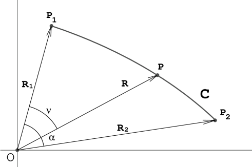
Fig 1: The geodesic $C$ and the angles $\alpha=\angle P_{1}OP_{2}$ and $\nu=\angle P_{1}OP$

On this way the following substantive items can be arrived at.

The ${\cal E}_{g}^{SR}$-Case Two-Point Distance $\Delta s$:

$$(\Delta s)^{2}=(F(g;R_{1}))^{2}+(F(g;R_{2}))^{2}-2F(g;R_{1})F(g;R_{2})\cosh\alpha.$$ (2.14)

The ${\cal E}_{g}^{SR}$-Case Scalar Product

$$<R_{1},R_{2}>=F(g;R_{1})F(g;R_{2})\cosh\alpha.$$ (2.15)

At equal vectors, the reduction

$$<R,R>=(F(g;R))^{2}$$ (2.16)

takes place, that is, the two-vector scalar product (2.1) reduces exactly to the squared FMF.

The ${\cal E}_{g}^{SR}$-Case Orthogonality

$$<R,R^{\perp}>=0.$$ (2.17)

Under the identification

$$|R_{1}\ominus R_{2}|=\Delta s$$ (2.18)

the formula (2.12) can be read as

The ${\cal E}_{g}^{SR}$-Case Cosine Theorem

$$|R_{1}\ominus R_{2}|^{2}=(F(g;R_{1}))^{2}+(F(g;R_{2}))^{2}-2<R_{1},R_{2}>.$$ (2.19)

From this we can also conclude that

The ${\cal E}_{g}^{SR}$-Case Pythagoras Theorem

$$|R\ominus R^{\perp}|^{2}=(F(g;R))^{2}+(F(g;R^{\perp}))^{2}$$ (2.20)

holds fine.

The symmetry

$$|R_{1}\ominus R_{2}|=|R_{2}\ominus R_{1}|$$ (2.21)

is obvious.

NOTE. One can easily execute the formula (2.14) from the representation (2.7) if one inserts (2.8) in (2.7), takes the case $s=\Delta s$, uses the equality

$$F(g;R_{2})=F_{\Delta s}$$

(see (2.11)), and resolves the resultant equation to find ($\Delta s)^{2}$.

Particularly, from (2.2) it directly ensues that the value of the angle $\alpha$ formed by a vector $R$ with the pseudo-Finsleroid $R^{N}$–axis is given by

$$\alpha=\displaystyle\frac{1}{h}\mathop{\rm arccosh}\nolimits\displaystyle\frac{A(g;R)}{\sqrt{B(g;R)}\ },$$ (2.22)

where $A$ is the function defined by Eq. (A.32), and with $(N-1)$–dimensional equatorial $\{{\bf R}\}$–plane of the pseudo-Finsleroid is prescribed as

$$\alpha=\displaystyle\frac{1}{h}\mathop{\rm arccosh}\nolimits\displaystyle\frac{L(g;R)}{\sqrt{B(g;R)}\ },$$ (2.23)

where $L$ is the function given by Eq. (A.33).

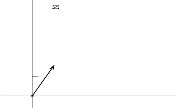
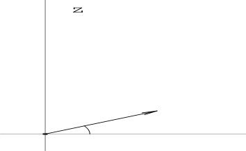
Fig 2: The angle cases (2.22) and (2.23), respectively.

Just the similar relationships are obtained in the co–approach. Given two co-vectors $P_{1}\in\hat{\cal V}_{g}$ and $P_{2}\in\hat{\cal V}_{g}$, the analogue of the formula (2.1) is the $\hat{\cal E}_{g}^{SR}$-scalar product

$$<P_{1},P_{2}>=H(g;P_{1})H(g;P_{2})\cosh\Bigl{[}\displaystyle\frac{1}{h}\mathop{\rm arccosh}\nolimits\displaystyle\frac{\hat{A}(g;P_{1})\hat{A}(g;P_{2})-h^{2}r^{be}P_{1b}P_{2e}}{\sqrt{\hat{B}(g;P_{1})}\,\sqrt{\hat{B}(g;P_{2})}}\Bigl{]},$$ (2.24)

which corresponds to the $\hat{\cal E}_{g}^{SR}$-angle

$$\hat{\alpha}(P_{1},P_{2})=\displaystyle\frac{1}{h}\mathop{\rm arccosh}\nolimits\displaystyle\frac{\hat{A}(g;P_{1})\hat{A}(g;P_{2})-h^{2}r^{be}P_{1b}P_{2e}}{\sqrt{\hat{B}(g;P_{1})}\,\sqrt{\hat{B}(g;P_{2})}}.$$ (2.25)

The complete analogue

$$|P_{1}\ominus P_{2}|^{2}=(H(g;P_{1}))^{2}+(H(g;P_{2}))^{2}-2H(g;P_{1})H(g;P_{2})\cosh\hat{\alpha}$$ (2.26)

to the formula (2.13) and the symmetry

$$|P_{1}\ominus P_{2}|=|P_{2}\ominus P_{1}|$$ (2.27)

hold fine.

In the pseudoeuclidean limit proper, the right-had parts in (2.2) and (2.25) takes on the ordinary pseudoeuclidean form:

$$\alpha(R_{1},R_{2})_{{\Bigl{|}\Bigr{.}}_{g=0}}=\mathop{\rm arccosh}\nolimits\displaystyle\frac{R_{1}^{0}R_{2}^{0}-r_{be}R_{1}^{b}R_{2}^{e}}{\sqrt{(R^{0}_{1})^{2}-r_{be}R_{1}^{b}R_{1}^{e}}\,\sqrt{(R_{2}^{0})^{2}-r_{be}R_{2}^{b}R_{2}^{e}}}$$

$$\hat{\alpha}(P_{1},P_{2})_{{\Bigl{|}\Bigr{.}}_{g=0}}=\mathop{\rm arccosh}\nolimits\displaystyle\frac{P_{10}P_{20}-r^{be}P_{1b}P_{2e}}{\sqrt{(P_{10})^{2}-r^{be}P_{1b}P_{1e}}\,\sqrt{(P_{20})^{2}-r^{be}P_{2b}P_{2e}}}.$$

Using (2.5) and (2.6) in (2.4) yields

$$R^{p}(s)=\displaystyle\frac{F_{s}}{k(s)\sqrt{B(g;R_{1})}}\displaystyle\frac{\sinh(h(\alpha-\nu))}{\sinh(h\alpha)}R^{p}_{1}+\displaystyle\frac{F_{s}}{k(s)\sqrt{B(g;R_{2})}}\displaystyle\frac{\sinh(h\nu)}{\sinh(h\alpha)}R^{p}_{2}+X(s)\delta^{p}_{N}$$ (2.28)

with

$$X(s)=-\displaystyle\frac{1}{2}g\displaystyle\frac{F_{s}}{k(s)}\Bigl{[}\displaystyle\frac{\sinh(h(\alpha-\nu))}{\sinh(h\alpha)}\displaystyle\frac{q_{1}}{\sqrt{B(g;R_{1})}}+\displaystyle\frac{\sinh(h\nu)}{\sinh(h\alpha)}\displaystyle\frac{q_{2}}{\sqrt{B(g;R_{2})}}-\displaystyle\frac{m(s)}{hF_{s}}\Bigr{]}.$$ (2.29)

Since the additional term $X(s)\delta^{p}_{N}$ has appeared in the right-hand part of (2.28), and the right-hand part in (2.29) does not vanish identically, we are to conclude that in general the vector $R^{p}(s)$ is not spanned by two end vectors $R^{p}_{1}$ and $R_{2}^{p}$. Therefore, in general the ${\cal E}_{g}^{SR}$-geodesic curves obtained are not plane curves.

The velocity components

$$U^{p}(s)\stackrel{{\scriptstyle\rm def}}{{=}}\displaystyle\frac{dR^{p}}{ds}$$ (2.30)

can conveniently be deduced from the equalities

$$U^{p}(s)=\mu^{p}_{j}(g;{\bf t}(s))\displaystyle\frac{dt^{j}}{ds},$$ (2.31)

where $\mu^{p}_{j}$ are the functions that are the quasi-pseudoeuclidean functions (B.13). Calculations show that

$$U^{p}(s)=\displaystyle\frac{b+s}{(F_{s})^{2}}R^{p}(s)+\displaystyle\frac{hF(g;R_{1})F(g;R_{2})\sinh\alpha}{k_{s}F_{s}\sinh(h\alpha)\,\Delta s}T^{p}(s)$$ (2.32)

with

$$T^{N}(s)=\displaystyle\frac{A(g;R_{2})}{h^{2}\sqrt{B(g;R_{2})}}\cosh(h\nu)-\displaystyle\frac{A(g;R_{1})}{h^{2}\sqrt{B(g;R_{1})}}\cosh(h(\alpha-\nu))$$ (2.33)

and

$$T^{a}(s)=\displaystyle\frac{1}{\sqrt{B(g;R_{2})}}\left[R_{2}^{a}+\displaystyle\frac{1}{2}g\displaystyle\frac{A(g;R_{2})}{h^{2}q}R^{a}(s)\right]\cosh(h\nu)$$

$$-\displaystyle\frac{1}{\sqrt{B(g;R_{1})}}\left[R_{1}^{a}+\displaystyle\frac{1}{2}g\displaystyle\frac{A(g;R_{1})}{h^{2}q}R^{a}(s)\right]\cosh(h(\alpha-\nu)).$$ (2.34)

It follows that

$${U^{p}(s)}_{{\Bigl{|}\Bigr{.}}_{g=0}}=\displaystyle\frac{R_{2}^{p}-R_{1}^{p}}{\Delta s},$$ (2.35)

and the contraction

$$R_{p}(s)U^{p}(s)=b+s$$ (2.36)

is valid, where $R_{p}$ are the covariant vector components (defined below (A.15)). Also,

$$g_{pq}(g;R(s))U^{p}(s)U^{q}(s)=1.$$ (2.37)

The initial-data solution

$$R_{2}^{p}=R_{2}^{p}(g;R_{1},U_{1},\Delta s)$$ (2.38)

can also be explicitly found, namely we get

$$R^{p}_{2}=\mu^{p}(g;t_{2})$$ (2.39)

with the functions

$$t_{2}^{i}=z(\Delta s)\sigma^{i}(g;R_{1})+n(\Delta s)\sigma^{i}_{q}(g;R_{1})U^{q}_{1},$$ (2.40)

$$z(\Delta s)=\displaystyle\frac{1}{h}\displaystyle\frac{\sinh(h\alpha)}{\sinh\alpha}+\displaystyle\frac{F(g;R_{2})}{F(g;R_{1})}\left[\cosh(h\alpha)-\displaystyle\frac{1}{h}\displaystyle\frac{\sinh(h\alpha)}{\sinh\alpha}\cosh\alpha\right],$$ (2.41)

$$n(\Delta s)=\displaystyle\frac{1}{h}\displaystyle\frac{\sinh(h\alpha)}{\sinh\alpha}\Delta s,$$ (2.42)

$$F(g;R_{2})=\sqrt{(F(g;R_{1}))^{2}+2b\Delta s+(\Delta s)^{2}},$$ (2.43)

$$b=R_{1q}U^{q}_{1},$$ (2.44)

and the angle value $\alpha$ can be taken as

$$\alpha=\mathop{\rm arccosh}\nolimits\displaystyle\frac{(F(g;R_{1}))^{2}+b\Delta s}{F(g;R_{1})F(g;R_{2})}.$$ (2.45)

The functions $\sigma^{i}$ and $\sigma^{i}_{q}$ are the inverses to $\mu^{i}$ and $\mu^{q}_{i}$, respectively.

Appendix A. Basic properties of the space ${\cal E}_{g}^{SR}$

Searching for extension of the pseudoeuclidean geometry in due Finsler-relativistic way, we should adapt constructions to the following decomposition

$${\cal V}_{g}={\cal S}_{g}^{+}\cup\Sigma_{g}^{+}\cup{{\cal R}_{g}}\cup\Sigma_{g}^{-}\cup{\cal S}_{g}^{-},$$ (A.1)

which sectors relate to the cases when the contravariant vector $R\in{\cal V}_{g}$ is respectively future–timelike, future–isotropic, spacelike, past–isotropic, and past–timelike. The respective co-analogue for the covariant vectors (momenta) $P\in\hat{\cal V}_{g}$ reads

$$\hat{\cal V}_{g}=\hat{\cal S}_{g}^{+}\cup\hat{\Sigma}_{g}^{+}\cup\hat{\cal R}_{g}\cup\hat{\Sigma}_{g}^{-}\cup\hat{\cal S}_{g}^{-}.$$ (A.2)

With this purpose, we introduce the following convenient notation:

$$G=g/h,$$ (A.3)

$$\qquad h\stackrel{{\scriptstyle\rm def}}{{=}}\sqrt{1+\displaystyle\frac{1}{4}g^{2}},$$ (A.4)

$$g_{+}=-\displaystyle\frac{1}{2}g+h,\qquad g_{-}=-\displaystyle\frac{1}{2}g-h,$$ (A.5)

$$G_{+}=g_{+}/h\equiv-\displaystyle\frac{1}{2}G+1,\qquad G_{-}=g_{-}/h\equiv-\displaystyle\frac{1}{2}G-1,$$ (A.6)

$$g^{+}=1/g_{+}=-g_{-},\qquad g^{-}=1/g_{-}=-g_{+},$$ (A.7)

$$g^{+}=\displaystyle\frac{1}{2}g+h,\qquad g^{-}=\displaystyle\frac{1}{2}g-h,$$ (A.8)

$$G^{+}=g^{+}/h\equiv\displaystyle\frac{1}{2}G+1,\qquad G^{-}=g^{-}/h\equiv\displaystyle\frac{1}{2}G-1.$$ (A.9)

We shall decompose vectors to select the timelike components and the three-dimensional spatial components: $R=\{R^{0},{\bf R}\}$ $P=\{P_{0},{\bf P}\}.$ In terms of the forms

$$B(g;R)=-\left(R^{0}+g_{-}|{\bf R}|\right)\left(R^{0}+g_{+}|{\bf R}|\right)\equiv-\left((R^{0})^{2}-gR^{0}\mbox{$|{\bf R}|$}-\mbox{$|{\bf R}|$}^{2}\right),$$ (A.10)

$$\hat{B}(g;P)=-\left(P_{0}-\displaystyle\frac{|{\bf P}|}{g^{+}}\right)\left(P_{0}-\displaystyle\frac{|{\bf P}|}{g^{-}}\right)\equiv-\left((P_{0})^{2}+gP_{0}\mbox{$|{\bf P}|$}-\mbox{$|{\bf P}|$}^{2}\right),$$ (A.11)

all the sectors entered the decompositions (A.1) and (A.2) can be embraced by one FMF

$$F(g;R)=\sqrt{|B(g;R)|}\,j(g;R)=\left|R^{0}+g_{-}|{\bf R}|\right|^{G_{+}/2}\left|R^{0}+g_{+}|{\bf R}|\right|^{-G_{-}/2},$$ (A.12)

where

$$j(g;R)=\left|\displaystyle\frac{R^{0}+g_{-}|{\bf R}|}{R^{0}+g_{+}|{\bf R}|}\right|^{-G/4},$$ (A.13)

and one FHF

$$H(g;P)=\sqrt{|\hat{B}(g;P)|}\,\hat{j}(g;P)=\left|P_{0}-\displaystyle\frac{|{\bf P}|}{g^{+}}\right|^{G^{+}/2}\left|P_{0}-\displaystyle\frac{|{\bf P}|}{g^{-}}\right|^{-G^{-}/2},$$ (A.14)

where

$$\hat{j}(g;P)=\left|\displaystyle\frac{P_{0}-\displaystyle\frac{|{\bf P}|}{g^{+}}}{P_{0}-\displaystyle\frac{|{\bf P}|}{g^{-}}}\right|^{G/4}.$$ (A.15)

By following the methods of the Finsler geometry, we use the definitions for the covariant vector

$$R_{p}\stackrel{{\scriptstyle\rm def}}{{=}}\displaystyle\frac{1}{2}\displaystyle\frac{\partial{F^{2}(g;R)}}{\partial{R^{p}}}\equiv P_{p}$$

and the FMT

$$g_{pq}(g;R)\stackrel{{\scriptstyle\rm def}}{{=}}\displaystyle\frac{1}{2}\,\displaystyle\frac{\partial^{2}F^{2}(g;R)}{\partial R^{p}\partial R^{q}}=\displaystyle\frac{\partial R_{p}(g;R)}{\partial R^{q}}.$$

Thus we get the Finsleroid-relativistic space

$${\cal E}_{g}^{SR}=\{{\cal V}_{g};\,F(g;R);\,g_{pq}(g;R);\,R\in{\cal V}_{g}\}$$ (A.16)

and the Finsleroid-relativistic co-space

$$\hat{\cal E}_{g}^{SR}=\{\hat{\cal V}_{g};\,H(g;P);\,g^{pq}(g;P);\,P\in\hat{\cal V}_{g}\}.$$ (A.17)

Special calculations can be used to verify the equalities

$$\det(g_{pq}(g;R))=-[j(g;R)]^{8}$$ (A.18)

and

$$\mathop{\rm sign}\nolimits(g_{pq})=\mathop{\rm sign}\nolimits(g^{pq})=(+---).$$ (A.19)

The following assertion is valid: for the Finsleroid space ${\cal E}_{g}^{SR}$ the Cartan torsion tensor

$$C_{pqr}\stackrel{{\scriptstyle\rm def}}{{=}}\displaystyle\frac{1}{2}\displaystyle\frac{\partial{g_{pq}}}{\partial{R^{r}}}$$

is of the special algebraic form

$$C_{pqr}=\displaystyle\frac{1}{N}\left(h_{pq}C_{r}+h_{pr}C_{q}+h_{qr}C_{p}-\displaystyle\frac{1}{C_{t}C^{t}}C_{p}C_{q}C_{r}\right),$$ (A.20)

where

$$C_{t}C^{t}=-\displaystyle\frac{N^{2}g^{2}}{4F^{2}}$$ (A.21)

and $N=4$.

Proof is gained by straightforward calculations on the basis of the explicit form of components of the FMT and the Cartan tensor (see more detail in [9–11]). Inserting (A.20)–(A.21) in the general expression for the curvature tensor

$$S_{pqrs}=C_{tqr}{C}_{p}^{t}{}_{s}-C_{tqs}{C}_{p}^{t}{}_{r}$$

yields the following simple result after rather simple straightforward calculations:

$$S_{pqrs}=S^{*}(h_{pr}h_{qs}-h_{ps}h_{qr})/F^{2}$$ (A.22)

with the constant

$$S^{*}=\displaystyle\frac{1}{4}g^{2}.$$ (A.23)

The tensor

$$h_{pr}\stackrel{{\scriptstyle\rm def}}{{=}}g_{pr}-l_{p}l_{r}$$ (A.24)

has been used, where $l_{p}=R_{p}/F(g;R)$ – the unit vector components.

The FMF (A.12) defines the pseudo-Finsleroid

$${\cal F}^{Relativistic}_{g}~{}:=\{R\in{\cal V}_{g}:F(g;R)\leq 1\}.$$ (A.25)

The associated indicatrix ${\cal I}_{g}$ defined by

$${\cal I}_{g}:=\{R\in{\cal V}_{g}:F(g;R)=1\}$$ (A.26)

is the surface of the pseudo-Finsleroid. With the given FHF (A.14), the body

$$\hat{\cal F}^{Relativistic}_{g}:=\{\hat{R}\in\hat{\cal V}_{g}:H(g;\hat{R})\leq 1\}$$ (A.27)

is called the co-pseudo-Finsleroid. The respective figuratrix introduced according to

$$\hat{\cal I}_{g}:=\{\hat{R}\in\hat{\cal V}_{g}:H(g;\hat{R})=1\}$$ (A.28)

is called the co-indicatrix.

From (A.22)–(A.24) it follows that in case of the Finsleroid space ${\cal E}_{g}^{SR}$ the indicatrix is a space of the constant negative curvature which value is equal to

$$R_{\rm Ind}=-\left(1+\displaystyle\frac{1}{4}g^{2}\right)\leq-1.$$ (A.29)

The respective equation of ${\cal F}_{g}$-geodesics is of the form

$$\frac{d^{2}R^{p}}{ds^{2}}+{C}_{q}^{p}{}_{r}(g;R)\displaystyle\frac{dR^{q}}{ds}\displaystyle\frac{dR^{r}}{ds}=0,$$ (A.30)

where $s$ is the parameter of the arc-length defined in accordance with the rule

$$ds\stackrel{{\scriptstyle\rm def}}{{=}}\sqrt{g_{pq}(g;R)dR^{p}dR^{q}}.$$ (A.31)

The use of the functions

$$A(g;R)=R^{0}-\displaystyle\frac{1}{2}g\mbox{$|{\bf R}|$},\qquad\hat{A}(g;P)=P_{0}+\displaystyle\frac{1}{2}g\mbox{$|{\bf P}|$}$$ (A.32)

and

$$L(g;R)=\mbox{$|{\bf R}|$}-\displaystyle\frac{1}{2}gR^{0},\qquad\hat{L}(g;P)=\mbox{$|{\bf P}|$}+\displaystyle\frac{1}{2}gP_{0}$$ (A.33)

is often convenient in various calculations.

In the limit $g\to 0$ the considered space degenerates to the ordinary pseudoeuclidean case:

$$B|_{{}_{g=0}}=-[(R^{0})^{2}-{\bf R}^{2}],\quad\hat{B}|_{{}_{g=0}}=-[(P_{0})^{2}-{\bf P}^{2}],$$

$$j|_{{}_{g=0}}=\hat{j}|_{{}_{g=0}}=1,\,F|_{{}_{g=0}}=\sqrt{|(R^{0})^{2}-{\bf R}^{2}|},$$

$$H|_{{}_{g=0}}=\sqrt{|(P_{0})^{2}-{\bf P}^{2}|},\quad g_{pq}|_{{}_{g=0}}=e_{pq},$$

$$g^{pq}|_{{}_{g=0}}=e^{pq},\quad C_{pqr}|_{{}_{g=0}}=0,\quad R_{\rm Ind}|_{{}_{g=0}}=-1.$$

Since at $g=0$ the space ${\cal E}_{g}^{SR}$ is pseudoeuclidean, then ${\cal I}_{g=0}$ is the ordinary unit hyperboloid.

Appendix B. Quasi-pseudoeuclidean transformation

Let us introduce the nonlinear transformation

$$t^{i}=\sigma^{i}(g;R)$$ (B.1)

with the functions

$$\sigma^{0}=\left|\displaystyle\frac{R^{0}+g_{-}|{\bf R}|}{R^{0}+g_{+}|{\bf R}|}\right|^{-G/4}\left(R^{0}-\displaystyle\frac{1}{2}g\mbox{$|{\bf R}|$}\right),\qquad\sigma^{a}=h\left|\displaystyle\frac{R^{0}+g_{-}|{\bf R}|}{R^{0}+g_{+}|{\bf R}|}\right|^{-G/4}R^{a};$$ (B.2)

$i,j,...=0,1,2,3$ and $a,b,...=1,2,3$. With the help of the transformartion, we can go over to from the variables $\{R^{p}\}$ to the new variables $\{t^{i}\}$. The inverse transformation

$$R^{p}=\mu^{p}(g;t)$$ (B.3)

involves the functions

$$\mu^{0}=\left|\displaystyle\frac{t^{0}-m}{t^{0}+m}\right|^{G/4}(t^{0}+\displaystyle\frac{1}{2}Gm),\qquad\mu^{a}=\displaystyle\frac{1}{h}\left|\displaystyle\frac{t^{0}-m}{t^{0}+m}\right|^{G/4}t^{a},$$ (B.4)

so that

$$t^{i}\equiv\sigma^{i}\left(g;\mu(g;t)\right),\qquad R^{p}\equiv\mu^{p}\left(g;\tau(g;R)\right).$$ (B.5)

The notation

$$m=\sqrt{|r_{ab}t^{a}t^{b}|}\in[0,\infty)$$

has been used; the constant $h$ is given by the formula (A.4).

Let us introduce the pseudoeuclidean metric function

$$S(t)\stackrel{{\scriptstyle\rm def}}{{=}}\sqrt{|e_{ij}t^{i}t^{j}|}\equiv\sqrt{|(t^{0})^{2}-m^{2}|}$$ (B.6)

$(e_{ij}={\rm diag}(1,-1,-1,-1)$ – the pseudoeuclidean metric tensor). It can readily be verified that the insertion of the the functions (B.2) in (B.6) yields the identity

$$F(g;R)=S(t)$$ (B.7)

with the function $F(g;R)$ which is exactly the FMF (A.12). In this way, we call (B.1)–(B.2) the quasi-pseudoeuclidean transformation.

The functions (B.2) are obviously homogeneous of degree 1 with respect to the variable  $R$:

$$\sigma^{i}(g;bR)=b\sigma^{i}(g;R),\qquad b>0,$$ (B.8)

from which it ensues that the derivatives

$$t_{p}^{i}(g;R)\stackrel{{\scriptstyle\rm def}}{{=}}\displaystyle\frac{\partial{\sigma^{i}(g;R)}}{\partial{R^{p}}}\equiv\sigma_{p}^{i}(g;R)$$ (B.9)

obey the identity

$$t_{p}^{i}(g;R)R^{p}=t^{i}.$$ (B.10)

Calculating the determinant gives merely

$$\det(t_{p}^{i})=j^{4}h^{3}.$$ (B.11)

Similarly,

$$\mu^{p}(g;bt)=b\mu^{p}(g;t),\qquad b>0,$$ (B.12)

$$\mu_{i}^{p}(g;t)\stackrel{{\scriptstyle\rm def}}{{=}}\displaystyle\frac{\partial{\mu^{p}(g;t)}}{\partial{t^{i}}},$$ (B.13)

and

$$\mu_{i}^{p}(g;t)t^{i}=R^{p}.$$ (B.14)

Next, let us now construct the tensor

$$n^{ij}(g;t)\stackrel{{\scriptstyle\rm def}}{{=}}t_{p}^{i}t_{q}^{j}g^{pq}.$$ (B.15)

Straightforward rather lengthy calculations result in the following simple representations

$$n^{ij}(g;t)=h^{2}e^{ij}-\displaystyle\frac{1}{4}g^{2}l^{i}l^{j},\qquad n_{ij}(g;t)=\displaystyle\frac{1}{h^{2}}e_{ij}+\displaystyle\frac{1}{4}G^{2}l_{i}l_{j}$$ (B.16)

($e_{ij}e^{jm}=\delta_{i}^{m}$ $n_{ij}n^{jm}=\delta_{i}^{m}$), where

$$l^{i}\stackrel{{\scriptstyle\rm def}}{{=}}t^{i}/S(t),\qquad l_{i}\stackrel{{\scriptstyle\rm def}}{{=}}e_{ij}l^{j}$$ (B.17)

are respective pseudoeuclidean unit vectors. For them the equalities

$$l^{i}l_{i}=1,\quad n_{ij}l^{j}=l_{i},\quad n^{ij}l_{j}=l^{i},\quad n_{ij}l^{i}l^{j}=1,\quad n_{ij}t^{i}t^{j}=S^{2}$$

are valid. The inversion of (B.15) can be written in the form

$$g_{pq}(g;R)=n_{ij}\left(g;\sigma(g;R)\right)t_{p}^{i}(g;R)t_{q}^{j}(g;R).$$ (B.18)

We also obtain

$$\det(n_{ij})=-h^{6}.$$ (B.19)

We call the tensor $\{n\}$ with the components (B.16) quasi-pseudoeuclidean metric tensor, and the very space

$${\cal K}_{g}:=\{{\cal Q};\,S(t);\,n_{ij}(g;t);\,t\in{\cal Q}\}$$ (B.20)

quasi-pseudoeuclidean space. The formulas (B.7) (B.15) show explicitly that space defined is quasi-pseudoeuclidean image of the Finsleroid-relativistic space ${\cal E}_{g}^{SR}$, such that when using the quasi-pseudoeuclidean transformations the studied Finsleroid-relativistic space ${\cal E}_{g}^{SR}$ transforms in the quasi-pseudoeuclidean space ${\cal K}_{g}=\sigma({\cal F}_{g})$ differed essentially from the pseudoeuclidean space ${\cal E}\equiv{\cal K}_{g=0}$.

Let us evaluate from the tensor (B.16) the associated Christoffel symbols

$${N}_{m}^{i}{}_{n}=n^{mk}N_{ikj},\quad N_{ikj}=\displaystyle\frac{1}{2}(n_{ik,j}+n_{jk,i}-n_{ij,k}).$$ (B.21)

We have subsequently

$$n_{ik,j}\stackrel{{\scriptstyle\rm def}}{{=}}\displaystyle\frac{\partial{n_{ik}}}{\partial{t^{j}}}=\displaystyle\frac{1}{4}g^{2}(H_{ij}L_{k}+H_{kj}L_{i})/S,$$ (B.22)

$$H_{mi}=e_{mi}-L_{m}L_{i}\equiv h^{2}(n_{mi}-L_{m}L_{i}),$$ (B.23)

$$L^{i}H_{ij}=0,$$ (B.24)

$$N_{mjn}=\displaystyle\frac{1}{4}G^{2}H_{mn}L_{j}/S,\qquad{N}_{m}^{i}{}_{n}=\displaystyle\frac{1}{4}G^{2}H_{mn}L^{i}/S,$$ (B.25)

and

$${N}_{i}^{m}{}_{j}(t)=\displaystyle\frac{1}{4}G^{2}L^{m}H_{ij}/S.$$ (B.26)

This entails the properties

$$t^{i}{N}_{i}^{m}{}_{j}=0,\qquad{N}_{i}^{j}{}_{j}=0.$$

References

[1]

H.  Busemann: Canad. J. Math. 1 (1949), 279.

[2]

H.  Rund: The Differential Geometry of Finsler spaces, Springer-Verlag, Berlin 1959.

[3]

G.S.  Asanov: Finsler Geometry, Relativity and Gauge Theories, D. Reidel Publ. Comp., Dordrecht 1985.

[4]

D. Bao, S.S.  Chern, and Z.  Shen: An Introduction to Riemann-Finsler Geometry,  Springer, N.Ẏ., Berlin, 2000.

[5]

G.S.  Asanov: Rep. Math. Phys. 45 (2000), 155; 47 (2001), 323.

[6]

G.S.  Asanov: arXiv:hep-ph/0306023, 2003; arXiv:math.MG/0402013, 2004;