$p$-Adic wavelet transform and quantum physics

Abstract

$p$-Adic wavelet transform is considered as a possible tool for the description of hierarchic quantum systems.

1 Introduction

Wavelet transform (WT) (see any general textbook [Dau92, Mal99] for the detailed review of the subject), as a generalization of windowed Fourier transform is widely used in various branches of physics, computing and image processing. Its tremendous success in localizing the singularities of fields and signals is mainly due to its mutual locality in coordinate and momentum: a local disturbance of wavelet coefficients affects the reconstructed image only locally, without spoiling the whole picture.

Formally the wavelet decomposition of a vector $\nu$ in a Hilbert space $\mathcal{H}$ is a decomposition with respect to the square-integrable representation $U(g)$ of the affine group

$$G:x^{\prime}=ax+b,\quad a,b\in\mathbb{R},a\neq 0,$$ (1)

acting transitively on $\mathcal{H}$ [GJP85], written as follows:

$$|\nu\rangle=\int_{G}U(g)|\psi\rangle d\mu_{L}(g)\langle\psi|U(g)|\nu\rangle,$$

where $d\mu_{L}(g)=\frac{dadb}{a^{2}}$ is a left-invariant measure on $G$ and $\psi\in\mathcal{H}$ is an appropriately chosen vector, called a basic wavelet.

In practical applications, $\mathcal{H}$ usually is the space of square-integrable functions ${L^{2}(\mathbb{R})}$, and the basic wavelet $\psi$ is a certain compactly supported function in it. The power of the wavelet transform is due to the fact that the analyzing window function $[U(a,b)\psi](x)=|a|^{-1/2}\psi\left(\frac{x-b}{a}\right)$ has the width varying with the scale parameter $a$, and thus works as a microscope that locally analyzes the details of a given scale.

Bearing in mind the application to the functions of $p$-adic argument rather than ${L^{2}(\mathbb{R})}$, we modify the definitions of direct and inverse WT in ${L^{1}(\mathbb{R})}$-norm as follows:

$$(W_{\psi}f)(a,b) = \int\frac{1}{a}\bar{\psi}\left(\frac{x-b}{a}\right)f(x)dx$$ (2)

$$f(x) = \frac{2}{C_{\psi}}\int_{0}^{\infty}\frac{da}{a^{2}}\int db(W_{\psi}f)(a,b)\psi\left(\frac{x-b}{a}\right),$$ (3)

where

$$C_{\psi}=\|\psi\|^{-2}\int d\mu_{L}(g)|\langle\psi|U(g)|\psi\rangle|^{2}.$$

For the case of affine group (1) $C_{\psi}=\int\frac{|\tilde{\psi}(\omega)|^{2}}{|\omega|}d\omega$, where tilde means the Fourier transform.

Before defining wavelet transform in $\mathcal{Q}_{p}$, it is worth noting that both wavelet transform and $p$-adic numbers provide hierarchic description of reality. Say, $p$-adic integers, defined by (10) below, for $p\!=\!2$ describe a point of the unit interval $[0,1)\!\in\!\mathbb{R}$ in terms of the embedded set of its vicinities, halved in size at each step. To some extent, a $p$-adic integer (10) labels an analog point in a $(d\!=p\!-\!2)$-dimensional simplex partitioned in a self-similar way into $p$ parts on each iteration, see Fig. 1 for two dimensional example. Since the $d$-dimensional sphere $S^{d}$ is homeomorphic to the boundary of $(d\!+\!1)$ dimensional simplex, it is possible to label the points of $S^{d}$ using the coordinates on that simplex.

The remainder of this paper is organized as follows. In Section 2 we review the basic facts on $p$-adic numbers, their geometrical interpretation and consider a few constructions of $p$-adic wavelet transform. An implementation of the $p$-adic WT with the Haar wavelet is presented. In Section 3, we define $p$-adic WT with Haar wavelet. Section 4 presents the Hilbert space of states of hierarchic quantum systems and considers possible links to $p$-adic wavelet transform. A generalization of quantum computation on qubit states is extended in Section 5 to quantum systems constructed from elementary units with $p\!>\!2$ states.

2 p-Adic wavelet transform

Prior to defining $p$-adic wavelet transform, let us review the basic facts about $p$-adic numbers. The results of any physical measurement can be expressed in terms of rational numbers $\mathbb{R}$. The construction of a theoretical model, first of all a description in terms of differential equations, ultimately requires an extension of this field. The first extension (made by Dedekind, viz. equivalence classes) means the incorporation of rational numbers. It is a completion of the field $\mathbb{Q}$ with respect to the standard norm $\mathbb{Q}\stackrel{{\scriptstyle|\cdot|}}{{\rightarrow}}\mathbb{R}$. However, this completion does not exhaust all possibilities. It is also possible to extend the field $\mathbb{Q}$ using the p-adic norm $|\cdot|_{p}$ (to be explained below):

$$\mathbb{R}\stackrel{{\scriptstyle|\cdot|}}{{\leftarrow}}\mathbb{Q}\stackrel{{\scriptstyle|\cdot|_{p}}}{{\rightarrow}}\mathcal{Q}_{p}.$$ (4)

This completion is called the field of $p$-adic numbers $\mathcal{Q}_{p}$. No other extensions of $\mathbb{Q}$ except those two exist due to the Ostrovski theorem [Ost18, BS66].

The $p$-adic norm $|\cdot|_{p}$ is defined as follows. Any nonzero rational number $x\in\mathbb{Q}$ can be uniquely written in the form

$$x=\frac{m}{n}p^{\gamma},$$ (5)

where integers $m$ and $n$ are not divisible by the prime integer $p\neq 1$, and $\gamma$ is an integer. The decomposition (5) provides a possibility to supply the field $\mathbb{Q}$ with the norm

$$|x|_{p}={\left|\frac{m}{n}p^{\gamma}\right|}_{p}\stackrel{{\scriptstyle def}}{{=}}p^{-\gamma},\qquad|0|_{p}\stackrel{{\scriptstyle def}}{{=}}0,$$ (6)

different from the standard one. The algebraic closure of the field $\mathbb{Q}$ in the norm $|\cdot|_{p}$ forms the field of $p$-adic numbers $\mathcal{Q}_{p}$.

Any $p$-adic number can be uniquely written in the form

$$x=\sum_{n=k_{min}}^{\infty}a_{n}p^{n},\qquad a_{n}\in\{0,1,\ldots,p-1\},\quad k_{min}>-\infty.$$ (7)

It is easy to see that $|xy|_{p}=|x|_{p}|y|_{p},$ but $|\cdot|_{p}$ is stronger than $|\cdot|$:

$$|x+y|_{p}\leq max(|x|_{p},|y|_{p})\leq|x|_{p}+|y|_{p},$$ (8)

and induces a non-Archimedian metric

$$d(x,y) := |x-y|_{p}$$ (9)

$$d(x,z) \leq max(d(x,y),d(y,z))\leq d(x,y)+d(y,z),$$

often called an ultrametric [RTV86]. With respect to the metric (9), the $\mathcal{Q}_{p}$ becomes a complete metric space. The maximal compact subring of $\mathcal{Q}_{p}$

$$\mathbb{Z}_{p}=\{x\in\mathcal{Q}_{p}:|x|_{p}\leq 1\}$$ (10)

is referred to as a set of p-adic integers. The field $\mathcal{Q}_{p}$ admits a positive Haar measure, unique up to normalization

$$d(x+a)=dx,\quad d(cx)=|c|_{p}dx,\quad x,a,c\in\mathcal{Q}_{p}.$$ (11)

The normalization is often chosen as $\int_{\mathcal{Z}_{p}}dx\equiv 1$.

The geometry induced by the distance $|x-y|_{p}$ is quite different from the Euclidean one: all $p$-adic triangles are equilateral; two $p$-adic balls may either be one within another or disjoint.

There is no unique definition of differentiation in the field $\mathcal{Q}_{p}$, but the Fourier transform exists and is used in $p$-adic field theory to construct the pseudo-differential operator

$$D\phi(x)\to|k|_{p}\tilde{\phi}(k).$$

The construction of the $p$-adic Fourier transform is essentially based on the group structure of the field $\mathcal{Q}_{p}$, viz. the group of additive characters

$$\chi_{p}(x):=\exp\bigl{(}2\pi\imath\{x\}_{p}\bigr{)},\quad\chi_{p}(a+b)=\chi_{p}(a)\chi_{p}(b),$$ (12)

(where $\{x\}_{p}$ denotes the fractional part of $x$: $\{x\}_{p}=a_{min}p^{k_{min}}+\ldots+a_{-1}p^{-1}$), is used to construct the Fourier transform

$$\tilde{\psi}(\xi)=\int_{\mathcal{Q}_{p}}\psi(x)\chi_{p}(\xi x)dx,\quad\psi(x)=\int_{\mathcal{Q}_{p}}\tilde{\psi}(\xi)\chi_{p}(-\xi x)d\xi.$$ (13)

The $n$-dimensional generalization is straightforward.

$$\mathcal{Q}_{p}\to\mathcal{Q}_{p}^{n},\quad x\to(x_{1},\ldots,x_{n}),\quad\xi\to(\xi_{1},\ldots,\xi_{n}),\quad\xi x\to(\xi,x)=\sum_{i}\xi_{i}x_{i}.$$

Now, let us show how $p$-adic coordinates can be used to label the points of ($d\!=\!p\!-\!2$)-dimensional manifolds. Let us consider a ($d\!=\!p\!-\!2$)-dimensional simplex, a triangle for $d\!=\!2$ is shown in Fig. 1.

Figure 1: The partition of a d-dimensional simplex ($d\!=\!p\!-\!2$) into $p$ equal parts.The case of $d\!=\!2$ is shown. If the the unit measure is assigned to the initial simplex, the volume of each subpart coincides with the norm of the $p$-adic number it is labeled by.

We can divide our 2d simplex, shown in Fig. 1, into into $p\!=\!4$ equal equilateral triangles and label them by 0,1,2,3. The initial triangle is therefore subdivided into $p\!=\!d\!+\!2$ equal parts; since the same procedure can be also applied to its parts we can move down ad infinum and label these parts as $a_{0},a_{1},\ldots$, where $0\leq a_{i}<p$. If we ascribe a measure $\mu(T_{0})=1$ to the initial triangle, when at the first stage we have $p$ triangles of the measure $1/p$ each, at the second stage $p^{2}$ triangles of the measure $1/p^{2}$ and so on. To meet this natural definition of the measure, we can label the sequences $\{a_{i}\}$ by $p$-adic integers. Generally, a $d$-dimensional simplex can be divided into $p=d+1$ equal parts, but to some extent we can consider $p$-adic balls as vicinities of points in a compact ultrametric space with a geometry similar to $S^{d}$ partitioning shown in Fig. 1.

Having defined the integration in $\mathcal{Q}_{p}$ by (11), we can formally generalize the continuous wavelet transform to the affine group acting in $\mathcal{Q}_{p}$ [Alt97]:

$$G:x^{\prime}=ax+b,\quad a,x,b\in\mathcal{Q}_{p},\quad a\neq 0.$$ (14)

As it follows from the group multiplication law

$$(a,b)(a^{\prime},b^{\prime})=(aa^{\prime},ab^{\prime}+b),$$

the left invariant measure on $p$–adic affine group (14), up to normalization, has the form

$$d\mu_{L}(a,b)=\frac{dadb}{|a|_{p}^{2}},$$ (15)

which provides

$$d\mu_{L}(aa^{\prime},ab^{\prime}+b)=\frac{|a|_{p}da^{\prime}|a|_{p}db^{\prime}}{|aa^{\prime}|_{p}^{2}}=\frac{da^{\prime}db^{\prime}}{|a^{\prime}|_{p}^{2}}.$$

To construct a counterpart wavelet transform (2,3) for the $p$-adic affine group (14), we use an obvious definition scalar product of complex-valued functions of $p$-adic arguments,

$$\langle f,g\rangle=\int_{\mathcal{Q}_{p}}\bar{f}(x)g(x)dx,$$

which provides a functional norm $\|f\|^{2}\equiv\langle f,f\rangle$. Thus the direct generalization of (2,3) takes the form

$$(W_{\psi}f)_{\mathcal{Q}_{p}}(a,b) = \int_{\mathcal{Q}_{p}}\frac{1}{a}\bar{\psi}\left(\frac{x-b}{a}\right)f(x)dx$$ (16)

$$f(x) = \frac{1}{C_{\psi}}\int_{\mathcal{Q}_{p}^{*}\times\mathcal{Q}_{p}}\psi\left(\frac{x-b}{a}\right)(W_{\psi}f)_{\mathcal{Q}_{p}}(a,b)\frac{dadb}{|a|_{p}^{2}},$$ (17)

where $\mathcal{Q}_{p}^{*}\equiv\mathcal{Q}_{p}\setminus 0$.

An analog of the complex-valued Morlet wavelet have been constructed by S.Kozyrev [Koz02].This complex valued wavelet is constructed from additive character (12) of the field $\mathcal{Q}_{p}$ used in $p$-adic Fourier transform, and has the form

$$\psi(x)=\chi(p^{-1}x)\Omega(|x|_{p}),\quad x\in\mathcal{Q}_{p},$$ (18)

where $\Omega(\cdot)$ is characteristic function of the unit interval in $\mathbb{R}$. The Kozyrev wavelets (18) are eigenfunctions of the Vladimirov p-adic pseudoderivative [VVZ94]:

$$D^{\alpha}\psi(x)=p^{\alpha}\psi(x),\quad D^{\alpha}f(x):=\frac{p^{\alpha}-1}{1-p^{-1-\alpha}}\int_{\mathcal{Q}_{p}}\frac{f(x)-f(y)}{|x-y|_{p}^{1+\alpha}}dy,$$ (19)

where $dy$ is the Haar measure on $\mathcal{Q}_{p}$.

3 p-Adic wavelet transform with Haar wavelet

Concerning the discrete implementation of the $p$-adic wavelet transform, the most evident implementation is that with Haar wavelet. Haar wavelet is the simplest case of the basic wavelet

$$h(x)=\begin{cases}1:&0<x<1/2\\ -1:&1/2\leq x<1\\ 0:&{\rm elsewhere}.\cr\end{cases}$$ (20)

Using the scale factor $a\!=\!2$, we easily obtain the discrete representation of the affine group (${L^{1}(\mathbb{R})}$ norm is used)

$$h^{j}_{k}(x)=2^{-j}h(2^{-j}x-k)$$

and the wavelet coefficients

$$d^{j}_{k}[f]=\int 2^{-j}h(2^{-j}x-k)f(x)dx.$$

Then, forward and backward discrete wavelet transform with the Haar wavelet can be then easily evaluated using the Laplacian pyramidal scheme

$$\begin{array}[]{lllllll}s^{0}&\to&s^{1}&\to&s^{2}&\to&\ldots\\ &\searrow&&\searrow&&\searrow&\\ &&d^{1}&&d^{2}&&\ldots\end{array},$$

where $s^{0}$ is the initial data set, and two projections

$$s_{k}^{j+1}=\frac{s^{j}_{2k}+s^{j}_{2k+1}}{2},\quad d_{k}^{j+1}=\frac{s^{j}_{2k}-s^{j}_{2k+1}}{2}$$ (21)

are evaluated on each step; $s^{j+1}$ is evidently the “blurred” version of the previous level coefficients $s^{j}$, with $d^{j+1}$ being the details blurred out. The reconstruction from the Haar wavelet decomposition (21) is

$$s^{j}_{2k+1}=s^{j+1}_{k}-d^{j+1}_{k},\quad s^{j}_{2k}=s^{j+1}_{k}+d^{j+1}_{k}.$$ (22)

Similar fast algorithms can be constructed for a $p$-adic Haar wavelet. We define an analog of the Haar wavelet in $\mathcal{Q}_{p}$ as

$$h(x)=\begin{cases}1&|x|_{p}<1\\ ``-1^{\prime\prime}&|x|_{p}\geq 1\end{cases},\quad x\in\mathcal{Q}_{p}$$ (23)

where “-1” means $(-1\!\in\!\mathbb{R})$ or $\bar{1}\!=\!(p-1)+(p-1)p+(p-1)p^{2}+\ldots$, depending on whether $h$ is a complex-valued $h:\mathcal{Q}_{p}\to\mathbb{C}$ or a $p$-adic-valued function $h:\mathcal{Q}_{p}\to\mathcal{Q}_{p}$ . In the latter case, the pyramidal algorithm (21,22) for the Haar wavelet is exactly reproduced in $p$-adic arithmetics

$$s_{k}^{j+1}=s_{2k+1}^{j}+s_{2k}^{j},\quad d_{k}^{j+1}=s_{2k+1}^{j}-s_{2k}^{j}\equiv s_{2k+1}^{j}+\bar{s}_{2k}^{j},$$ (24)

with the reconstruction formulae

$$s^{j}_{2k+1}=\frac{s^{j+1}_{k}+d^{j+1}_{k}}{2},\quad s^{j}_{2k}=\frac{s^{j+1}_{k}+\bar{d}^{j+1}_{k}}{2}.$$ (25)

4 Hierarchic states of quantum systems

The quantum mechanical description based on the Schrödinger equation is formally applicable to any physical system from elementary particles to macroscopic bodies. However, it is technically impossible to account for each electron wave function in a living cell or in a microprocessor, or even in a big cluster of atoms. The methods of quantum statistical mechanics are of little use here, for most quantum systems of practical interest are far from statistical equilibrium.

At the same time, the problem of quantum description of mesoscopic objects, such as clusters of atoms and living cells, are becoming of steady practical interest for high-performance computing and biotechnology. Fortunately, there is a way to construct the wave functions of composite objects without taking the direct product of all component wave functions. As we always see, the Nature has clearly manifested its hierarchic structure: an electron is part of atom, an atom is part of a molecule etc.. This suggests that instead of taking the direct product of the component wave functions, we can represent the wave function of a composite system in a hierarchic form, successively taking into account the states of all systems our system is part of.

This suggests an idea of the hierarchic wave function [Alt03]. Let the system $C_{1}$ consist of two subsystems $B_{1}$ and $B_{2}$, each of those in turn consists of two subsystems, etc., see Fig. 2.

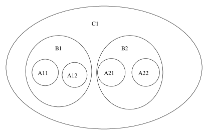
Figure 2: The structure of binary hierarchic system

To describe the binary hierarchic system shown in Fig. 2, we need a collection of wave functions

$$\Psi=\{\psi_{C_{1}},\{\psi_{C_{1}B_{1}},\psi_{C_{1}B_{2}}\},\{\psi_{C_{1}B_{1}A_{11}},\psi_{C_{1}B_{1}A_{12}},\psi_{C_{1}B_{2}A_{21}},\psi_{C_{1}B_{2}A_{22}}\}\},$$ (26)

where $\psi_{C_{1}}$ is the wave function of the whole (labeled by $C_{1}$), and $\psi_{C_{1}B_{1}}$ is the wave function of a component $B_{1}$ belonging to the entity $C_{1}$. The subsystem $B_{1}$ of $C_{1}$ described by the wave function $\psi_{C_{1}B_{1}}$ is not the same as a free system $B_{1}$ described by wave function $\psi_{B_{1}}$; e.g. an electron in atom is not the same as a free electron. The component wave function, that completely determines the state of the subsystem $A_{11}$ is then $(\psi_{C_{1}},\psi_{C_{1}B_{1}},\psi_{C_{1}B_{1}A_{11}})$. If required, the density matrix of such a system can be obtained by averaging over degrees of freedom of $C_{1}$ and $B_{1}$, but not the $B_{2}$, see [Alt03] for details.

Evidently, the binary tree structure presented above is a mathematical idealization: there is no a priory reason for the subsystem to have exactly the same number of parts as the system it is part of. This idealization, however, seems to be a good starting point to build a Hilbert space of states of hierarchic system. Having the same number of parts at each hierarchy level, and thus being self-similar, the presented construction of the hierarchic wave function gives us a quantum mechanics on $\mathcal{Q}_{p}$, where $p$ is the number of subparts.

Let us consider the Hilbert space of hierarchic wave functions [Alt03]. If $\Psi_{1}$ and $\Psi_{2}$ are two hierarchic wave functions (describing the same type hierarchic objects), then the superposition principle requires their linear combination to be in the same Hilbert space

$$\Psi_{1},\Psi_{2}\in\mathcal{H},a,b\in\mathbb{C}\Rightarrow\Psi=a\Psi_{1}+b\Psi_{2}\in\mathcal{H}.$$

For instance, if

$$\Psi_{1} = \{\psi_{B_{1}},\{\psi_{B_{1}A_{1}},\ldots,\psi_{B_{1}A_{N}}\},\ldots\},$$

$$\Psi_{2} = \{\psi_{D_{1}},\{\psi_{D_{1}C_{1}},\ldots,\psi_{D_{1}C_{N}}\},\ldots\},$$

then their linear combination is

$$\Psi=a\Psi_{1}+b\Psi_{2}=\{a\psi_{B_{1}}\!+\!b\psi_{D_{1}},\{a\psi_{B_{1}A_{1}}\!+\!b\psi_{D_{1}C_{1}},\ldots,a\psi_{B_{1}A_{N}}\!+\!b\psi_{D_{1}C_{N}}\},\ldots\}.$$ (27)

The scalar product is defined componentwise:

$$\langle\Psi_{1}|\Psi_{2}\rangle=\langle\psi_{B_{1}}|\psi_{D_{1}}\rangle+\sum_{i=1}^{N}\langle\psi_{B_{1}A_{i}}|\psi_{D_{1}C_{i}}\rangle+\ldots.$$ (28)

The norm of the vector in hierarchic space defined by scalar product is a sum of norms of all components:

$$||\Psi||^{2}=\langle\Psi_{1}|\Psi_{1}\rangle=\langle\Psi_{B_{1}}|\Psi_{B_{1}}\rangle+\sum_{i=1}^{N}\langle\Psi_{B_{1}A_{i}}|\Psi_{B_{1}A_{i}}\rangle+\ldots.$$ (29)

For a self-similar partitioning, if the number ($p$) of subparts is the same at all hierarchic levels, we can easily cast the properties (27-29) for the wave functions of $p$-adic argument $x\in\mathcal{Z}_{p}$. Let

$$x=a_{0}+a_{1}p+a_{2}p^{2}+\ldots,\quad 0\leq a_{i}<p$$ (30)

Then, we can define the hierarchic wave function component as

$$\Psi(x\in\mathcal{Z}_{p})=\{\psi_{a_{0}},\psi_{a_{0},a_{1}},\psi_{a_{0},a_{1},a_{2}},\ldots\}.$$ (31)

with normalization condition

$$\int_{\mathcal{Z}_{p}}\bar{\Psi}(x)\Psi(x)dx=1.$$ (32)

At this point we ought to mention the geometric aspect of the hierarchic wave function (31). If $x\!=\!a_{0}$ labels an entity, and $x^{\prime}\!=\!a_{0}\!+\!a_{1}p$ labels the parts of this entity, then the Haar measure $dx$ normalized as $\int_{\mathcal{Z}_{p}}dx\!=\!1$ provides that the measure the wave function $\psi_{a_{0}a_{1}}$ is integrated over is exactly $1/p$ of the measure of the entity $a_{0}$. This impose a particular geometry to the quantum mechanics of hierarchic wave functions $\eqref{pvf}$, which may, or may not, correspond to physical reality.

The second quantization on hierarchic states also has its own peculiarities. To create a state vector (26) of a hierarchic state, we have first to create the entity ($C_{1}$), and only then, we can create its parts acting by appropriate creation operators to the state $|C_{1}\rangle$.

$$a^{+}(C_{1})|0\rangle=|C_{1}\rangle,a(C_{1})|C_{1}\rangle=|0\rangle,a(C_{1})|0\rangle=0|0\rangle,$$

$$a^{+}(B_{i})|C_{1}\rangle=\{|C_{1}\rangle,|C_{1}B_{i}\rangle\},a(C_{1})\{|C_{1}\rangle,|C_{1}B_{i}\rangle\}=|B_{i}\rangle.$$ (33)

The latter equation (33) means the annihilation of the entity $C_{1}$ in a system comprised by components $B_{i}$: this is a decay of $C_{1}$ into components. The possible action of annihilation operator of a part $B_{i}$ in entity $C_{1}$

$$a(B_{i})\{|C_{1}\rangle,|C_{1}B_{i}\rangle\}=|C_{1}\rangle\quad(?)$$

is questionable.

If a toy model with the same number of parts at each hierarchy level is considered, the second quantization rules (33) provide a second quantization for the state vectors labeled by $p$-adic numbers. The hierarchic state vector can be created by sequential action of creation operators

$$|x\rangle=|a_{0}a_{1}a_{2}\ldots\rangle=\ldots a^{+}(a_{2})a^{+}(a_{1})a^{+}(a_{0})|0\rangle,$$ (34)

where second quantization $[a(i),a^{+}(j)]=\delta_{ij}$ is defined on the cyclic group $Z_{p}$ rather than a ring of $p$-adic integers.

5 Qubits and $p$-qubits

Qubit, a quantum analog of a classical bit, is a superposition of any two orthogonal quantum states, labeled as “0” and “1” for definiteness

$$|x\rangle=\alpha_{0}|0\rangle+\alpha_{1}|1\rangle.$$ (35)

Qubit is an elementary unit of quantum information. Strings of qubits

$$|x_{1},\ldots,x_{n}\rangle\equiv|x_{1}\rangle\otimes\ldots\otimes|x_{n}\rangle$$

are considered as analogues of classical computer registers. The general review in quantum information can be found elsewhere, see e.g. [NC00].

The idea of qubit, a superposition of two quantum states, comes from the fact that it is easy to prepare such states, e.g. a spin system or a two-level atom. Nevertheless, quantum systems with more than two orthogonal states are also known: the Potts model, atoms with 3 and more states etc.. Interestingly, it is very likely that the processing of genetic information in living cell operates as a quantum information processing in mod 4 or mod 5 arithmetics [AFO03]. So, we need a generalization of qubit to a superposition of ($p\!>\!2$) orthogonal quantum states. We will call it $p$-qubit.

A particular generalization of this type, a pentabit $p\!=\!5$, has been proposed in [AFO03]

$$|\phi\rangle=\alpha_{0}|0\rangle+\alpha_{1}|A\rangle+\alpha_{2}|C\rangle+\alpha_{3}|T\rangle+\alpha_{4}|G\rangle,$$ (36)

where $A,C,T,G$ stand for the four nucleotides (adenine, cytosine, thymine, guanine), and $0$ means the vacuum state, or a gap in a nucleotide sequence. The particular correspondence between nucleotides and the cyclic group $Z_{5}$ comes from biochemical properties of four nucleotides. Since $A$ and $G$ are purines and $C$ and $T$ are pyrimidines, the wave functions of $A$ and $G$ ($C$ and $T$, respectively) should not be very different from each other [Pat01]; thus it seems reasonable to use representation providing $A+G=0,T+C=0$, as chosen above in (36).

A string of such p-qubits can be subjected to all standard operations of quantum computing, including quantum Fourier transform and quantum wavelet transform, with the only exception that mod 2 operations will be substituted by mod $p$ operations. If a nucleotide sequence is considered as such a string ($p=5$), $p$-adic quantum computing may be a biocomputing.

Computational basis.

Similar to the traditional binary quantum computing, we can define functions and operators acting on $p$-qubits. Let

$$|x\rangle\otimes|s\rangle,\quad x,s=0,\ldots,p-1$$ (37)

be a computational basis. Let $f(x)$ be a mapping $Z_{p}\to Z_{p}$. The function $f$ can be then represented by an operator

$$U_{f}|x\rangle\otimes|s\rangle=|x\rangle\otimes|s\oplus f(x)\rangle.$$ (38)

Walsch-Hadamard transform.

For each $p$-qubit $|x\rangle$ we can define a Hadamard transform

$$|x\rangle\to H|x\rangle=\frac{1}{\sqrt{p}}\sum_{y=0}^{p-1}(-1)^{x\otimes y},|y\rangle$$ (39)

where $\otimes$ means mod $p$ product. The Hadamard state $H|x\rangle$ for a $p$-qubit $|x\rangle$ is therefore a quantum superposition of all $p$-qubit states, labeled by $0\!\leq\!y\!<p$, each taken with its parity with respect to $|x\rangle$. For a sequence of $n$ p-qubits $|X\rangle=|x_{1},\ldots,x_{n}\rangle$, therefore, the Hadamard transform is given by

$$|X\rangle\to H|X\rangle=\frac{1}{\sqrt{p^{n}}}\sum_{y\in\omega}(-1)^{\bar{x}\cdot\bar{y}}|Y\rangle,$$ (40)

where $\bar{x}\cdot\bar{y}$ is bitwise dot product mod p and the sum is taken over all $p^{n}$ sequences $|Y\rangle$ consisting of $n$ p-qubits.

Quantum Fourier transform.

Starting from standard form of the Fourier transform of a vector in Hilbert space used in quantum computing

$$F|x\rangle=\sum_{y}|y\rangle\exp(2\pi\imath\frac{xy}{\omega})$$ (41)

which is used for the sequences of fixed length of $n$ $p$-qubits (the total number of all this sequences is $\omega=p^{n}$), we can produce Fourier transform of any function

$$\begin{array}[]{lcl}F|\Psi_{f}\rangle&=&F\sum_{x}|x\rangle\otimes|f(x)\rangle=\sum_{x}F|x\rangle\otimes|f(x)\rangle\\ &=&\sum_{x,y}|y\rangle\exp(2\pi\imath\frac{xy}{\omega})\otimes|f(x)\rangle=\sum_{y}|y\rangle\otimes|g(y)\rangle,\end{array}$$ (42)

where $g(y)$ is the Fourier transform of $f(x)$. Further applications of $p$-qubits to quantum computing, quantum database search, quantum cryptography etc.can be considered in a straightforward way following the known algorithms for traditional qubits ($p=2$).

6 Conclusion

The origin of space-time geometry from a set of relations between discrete objects by Big Bang or by other scenario is a challenging problem of quantum field theory and cosmology. The studies in this field give rise both to the development of new field theoretical methods related to quantum cosmology and to the development of new mathematical methods based on number theory, that can be used in different fields from information protection and coding theory to molecular biology. This paper, being partially based on physical intuition rather than rigorous axiomatics, makes in attempt to outline some multiscale methods based on on the $p$-adic generalization of the wavelet transform, the tool widely used in signal processing and data compression. We hope this research will be followed by more rigorous mathematical consideration of problems and algorithms outlined above in this paper.

The other point of this paper was to attract attention to the possible generalization of quantum computing ideas to the quantum systems with $p>2$ orthogonal quantum states. Such systems, if organized in hierarchic structures, could be used for the hierarchic information storage. From mathematical point of view, the quantum states of those hierarchic structures can be discribed by wave functions depending on $p$-adic argument, and thus providing a new intriguing application of $p$-adic quantum mechanics.

References

• [AFO03] M.V. Altaisky, F.P. Filatov, and V.Yu. Ovodkov. Genetic information and quantum computing. Vestn. Novykh Med. Tekhnol., 10(4):5–8, 2003.
• [Alt97] M.V. Altaiski. $p$-adic wavelet decomposition vs fourier analysis on spheres. Indian J. of Pure and Appl. Math., 28(2):195–207, 1997.
• [Alt03] M.V. Altaisky. Quantum states of hierarchic systems. Int. J. Quantum Information, 1(2):269–278, 2003.
• [BS66] Z.I. Borevich and I.R. Schafarevich. Number Theory. Academic Press, New York, 1966.
• [Dau92] I.Β Daubechies. Ten lectures on wavelets. S.I.A.M., Philadelphie, 1992.
• [GJP85] A.Β Grossmann, Morlet J., and T.Β Paul. Transforms associated to square integrable group representations. i. general results. J. Math. Phys., 26:2473–2479, 1985.
• [Koz02] S.Β Kozyrev. Wavelet analysis as a p-adic spectral analysis. Izvestia Akademii Nauk Seria Math., 66(2):149–158, 2002.
• [Mal99] S.Β Mallat. A wavelet tour of signal processing. Academic Press, 1999.
• [NC00] M.A. Nielsen and I.L. Chuang. Quantum computation and quantum information. Cambridge University Press, 2000.
• [Ost18] A.Β Ostrowski. Acta Math., 41:271, 1918.
• [Pat01] A.Β Patel. Why genetic information processing could have a quantum basis. J.Biosciences., 26:145–151, 2001.
• [RTV86] R.Β Ramal, G.Β Toulouse, and M.A. Virasoro. Ultrametricity for physisists. Rev. Mod. Phys., 58:765–788, 1986.
• [VVZ94] V.S. Vladimirov, I.V. Volovich, and E.I. Zelenov. $p$–Adic numbers in mathematical physics. World Scientific, Singapore, 1994.