Integral representation of one dimensional three particle scattering for $\delta$ function interactions

A. Amaya-Tapia1, G. Gasaneo2,3, S. Ovchinnikov4, J. H. Macek2,4 and S. Y. Larsen5
Abstract

The Schrรถdinger equation, in hyperspherical coordinates, is solved in closed form for a system of three particles on a line, interacting via pair delta functions. This is for the case of equal masses and potential strengths. The interactions are replaced by appropriate boundary conditions. This leads then to requiring the solution of a free-particle Schrรถdinger equation subject to these boundary conditions. A generalized Kontorovich - Lebedev transformation is used to write this solution as an integral involving a product of Bessel functions and pseudo-Sturmian functions. The coefficient of the product is obtained from a three-term recurrence relation, derived from the boundary condition. The contours of the Kontorovich-Lebedev representation are fixed by the asymptotic conditions. The scattering matrix is then derived from the exact solution of the recurrence relation. The wavefunctions that are obtained are shown to be equivalent to those derived by McGuire. The method can clearly be applied to a larger number of particles and hopefully might be useful for unequal masses and potentials.

1 Centro de Ciencias Fรญsicas, UNAM, AP 48-3,Cuernavaca, Mor. 62251, Mรฉxico.

2 Department of Physics and Astronomy, University of Tennessee, Knoxville, TN 37996-1501, USA.

3 Departamento de Fรญsica, Universidad Nacional del Sur, Av. Alem 1253, (8000) Bahรญa Blanca, Buenos Aires, Argentina.

4 Oak Ridge National Laboratory, PO Box 2008, Oak Ridge, Tennessee 37831, USA

5 100 Forest Place, Apt. 1305, Oak Park, IL 60301, USA.

Introduction

Three-body systems and processes are of fundamental interest in physics [1]. One of these, with which a number of us have been concerned, is the recombination of three-particles to a dimer plus a free particle, in a many body system forming a Bose-Einstein condensate [2]. The condensate is not the lowest state of the system, but a metastable state. The 3-body recombination is the dominant mechanism for cooling and lowering the overall energy of the system.

Experimental and theoretical studies have shown that this recombination rate depends mainly on the two-body scattering length $a$ [3, 4, 5, 6, 2], as the collision energy is low and the interaction is weak - owing to large interparticle distances, and on the bound state energies.

This would suggest that zero-range potentials (ZRP), defined in terms of the scattering length [7],

$$\lim_{r\rightarrow 0}\left[\frac{1}{r\psi}\frac{\partial\left(r\psi\right)}{\partial r}\right]=-1/a.$$ (1)

can be applied to model the interaction between the particles of the condensate. It has been shown by Nielsen and Macek using the hidden crossing technique that the ZRP describes properly the recombination transition in a system of three 4He atoms [2]. Also, Gasaneo and Macek showed that the ZRP gives a quite good representation for the adiabatic potential of the same system [8]. A closed form solution for a system of three-particles interacting via a ZRP has been recently presented by Gasaneo et al [9]. The fragmentation process ย 4He${}_{2}+\leavevmode\nobreak\ ^{4}$He$\longrightarrow\leavevmode\nobreak\ ^{4}$He$+\leavevmode\nobreak\ ^{4}$He$+\leavevmode\nobreak\ ^{4}$He was studied and relatively good agreement was found when compared with the hidden crossing calculations.

In this paper, we seek to apply our techniques to a famous model: 3 particles in one dimension, subject to pair delta-function interactions. For this model, introduced by McGuire [10], one can obtain exact solutions for the wave functions, the scattering matrix and the binding energies, in the case of particles of identical masses and equally weighted interactions. As such it has been extended to a larger number of particles [11], using Betheโ€™s Ansatz [12], and also found to be exceedingly useful when used as a test-bed for the development of a number of different methods (pertubative, Faddeev, hyperspherical adiabatic, etc.) [13].

Here, we note that using ZRP and (1), in 3-dimensions, leads to the Thomas effect and the collapse of the 3-body ground state [14]. However, in one dimension, an equation similar to (1) - with $a$ not the scattering length - provides boundary conditions which correctly characterizes the wave functions and replace the use of the $\delta$-function interactions, and should therefore again give us exact results. One of these, though, is that the recombination rate, for this model, is exactly zero.

In section II we propose a solution, written in integral form, for the free particle Schrรถdinger equation, written in hyperspherical coordinates. A linear combination of free particle solutions can then be found to satisfy the boundary condition that we alluded to earlier, and thus provide us with the solution of the problem with interaction. The requirement that the wave function satisfy the boundary conditions leads us to one of the important results of this paper, namely that the weight of the free particle solutions, in the integral form, satisfies a recurrence relation similar to that obtained in the refs. [15] and [9].

In section III the method is applied to a particular case in which two of the particles are bound. It is shown that the recurrence relation, defining the coefficient of the free-particle expansion, can be solved in closed form and, thus, the scattering matrix is also obtained in a closed form. This allows us to have a detailed test of our method. In this section it is also shown that the wave function obtained is equivalent to the McGuire plane wave solution, and that our expression for the ${\mathcal{S}}$ matrix is the matrix obtained by McGuire, in the particular case discussed in this paper. In section IV the relation between the hyperspherical adiabatic approach and the present one is discussed.

In Appendix A, the pseudo-Sturmian functions are derived. In Appendix B, the wave function is written as the symmetric wave plane in cartesian coordinates.

Exact Integral Representation

To begin the study of the three identical-particle system (therefore with equal masses), consider the center of mass and Jacobi coordinates,

$\displaystyle r$ $\displaystyle=$ $\displaystyle\frac{1}{3}(x_{1}+x_{2}+x_{3}),$
$\displaystyle\eta$ $\displaystyle=$ $\displaystyle\sqrt{\frac{1}{2}}(x_{1}-x_{2}),$
$\displaystyle\xi$ $\displaystyle=$ $\displaystyle\sqrt{\frac{2}{3}}\left(\frac{x_{1}+x_{2}}{2}-x_{3}\right)$ (2)
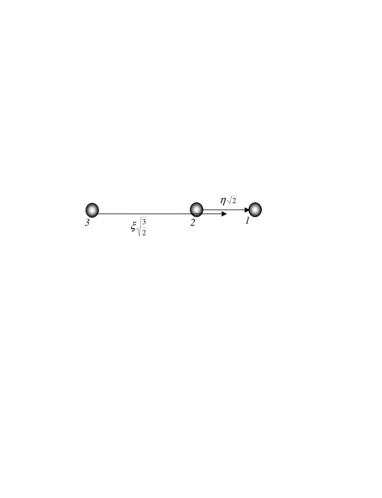
Figure 1: One of three sets of Jacobi coordinates for the three particles.
Refer to caption

the $x_{i}\,$ give us the locations of the 3 particles along the line, see Fig. 1 . Using polar coordinates, the 2 Jacobi variables allow us to define, in turn, a hyper radius $R$ and an angle $\theta$ as

$$\eta=R\cos\theta\qquad\qquad\xi=R\sin\theta$$ (3)

where $-\pi<\theta\leq\pi\,\,$and$0\leq R<\infty$. In terms of these coordinates the Schrรถdinger equation for the โ€˜relativeโ€™ system can be written as

$$H\Psi\left(R,\theta\right)=(\frac{2m}{\hbar^{2}})\,E\Psi\left(R,\theta\right)$$ (4)

where

$$H=-\left(\frac{1}{R}\frac{\partial}{\partial R}R\frac{\partial}{\partial R}+\frac{1}{R^{2}}\frac{\partial^{2}}{\partial\theta^{2}}\right)+\frac{1}{R}C\left(\theta\right).$$ (5)

The function $C\left(\theta\right)$ is defined by

$$C\left(\theta\right)=\frac{\pi}{3}c\sum\limits_{j=0}^{5}\,\delta\left(\theta-\theta_{j}\right),$$ (6)

where the coefficient $c$ equals $(3/\pi\sqrt{2})(2m/\hbar^{2})g$, $g$ being the strength of the interactions. This $c$ is negative for attractive interactions and positive for repulsive ones. The angles $\theta_{j}$ equal $(2j+1)\pi/6$. The lines $\theta=\theta_{j}$ divide the $(\rho,\theta)$ plane in six regions. In each region the order of particles is fixed, so that between $\theta_{4}$ and $\theta_{5}$, $x_{1}<x_{2}<x_{3}$, etc. A different permutation of particles is associated to each region. >From now on, we will choose the units such that $2m=1$ and $\hbar=1$. In each sector, we now seek a free particle solution that satisfies the boundary condition that will replace the effect of the potential, i.e.

$$\lim_{\theta^{-}\rightarrow\theta_{j}}\left[\frac{1}{R\Psi(R,\theta)}\frac{\partial\Psi(R,\theta)}{\partial\theta}\right]=-\frac{1}{a},$$ (7)

where $\theta^{-}=\theta<\theta_{j}\;j=0,1,...,5$. In Eq.(7) $a=(6/\pi c)$ does not depend on $j$ because all the strengths of the interactions and all the masses are equal. Writing a solution for the free particle system as the product $\psi_{free}\left(R,\theta\right)=\Theta\left(\nu,\theta\right)R^{1/2}{\mathcal{R}}_{\nu}\left(\mathrm{K}R\right)$, where $\mathrm{K}^{2}=E$, leads to the set of free particle equations

$\displaystyle\left.\frac{R^{2}}{R^{-1/2}Z_{\nu}\left(\mathrm{K}R\right)}\left[\frac{\partial^{2}}{}{\partial R^{2}}+\mathrm{K}^{2}\right]R^{-1/2}Z_{\nu}\left(\mathrm{K}R\right)\right.$
$\displaystyle\left.=\frac{-1}{\Theta(\nu,\theta)}\left(\frac{\partial^{2}}{}{\partial\theta^{2}}+\frac{1}{4}\right)\Theta(\nu,\theta)=\nu^{2}-\frac{1}{4}\right.,$ (8)

where $Z_{\nu}\left(\mathrm{K}R\right)=R^{1/2}{\mathcal{R}}_{\nu}\left(\mathrm{K}R\right)$ is a Bessel function and $\nu$ a separation constant. If for the $\Theta\left(\nu,\theta\right)$ functions we choose the pseudo-Sturmian functions $S(\nu,\theta)$, defined, for fixed $\nu$, as the solutions of

$$-\left[\frac{\partial^{2}}{\partial\theta^{2}}+\frac{1}{4}-\rho\left(\nu\right)C\left(\theta\right)\right]S(\nu,\theta)=\left(\nu^{2}-\frac{1}{4}\right)S(\nu,\theta),$$ (9)

then the functions $\psi_{free}\left(\theta,R\right)=S(\nu,\theta)Z_{\nu}\left(\mathrm{K}R\right)$ are solutions of the Schrรถdinger equation Eq.(4) for values of $\rho\left(\nu\right)=R.$ Note that Eq.(9) may be replaced by the relation

$$\left[\frac{\partial^{2}}{\partial\theta^{2}}+\nu^{2}\right]S(\nu,\theta)=0$$ (10)

subject to the boundary conditions

$$\lim_{\theta^{-}\rightarrow\theta_{j}}\left[\frac{1}{\rho\left(\nu\right)}\frac{1}{S(\nu,\theta)}\frac{\partial S}{\partial\theta}(\nu,\theta)\right]=-\frac{1}{a},\;j=0,1,...,5.$$ (11)

In the last equation, we assumed that $S(\nu,\theta)$ is symmetric about each line $\theta=\theta_{j}$.

We now propose to write the general wave function of the system as a Kontorovich-Lebedev transform, in terms of the base functions just discussed, that is, as

$$\Psi(R,\theta)=\int_{\varsigma}d\nu A(\nu)S\left(\nu,\theta\right)Z_{\nu}(\mathrm{K}R),$$ (12)

provided that its derivative satisfies the boundary conditions, i.e. Eq.(7). The contour of integration must be chosen so that the wave function has the correct asymptotic behaviour.

Following the reasoning of Gasaneo et al [8], we will now show that the boundary conditions, Eq.(7), โ€†โ€†can be transformed into a recurrence relation for $A\left(\nu\right)$. First, we substitute Eq.(12) in Eq.(7), and then interchange the order in which the integral and the derivative are taken, to obtain for each $j$

$\displaystyle\left.\lim_{\theta^{-}\rightarrow\theta_{j}}\int_{\varsigma}d\nu A(\nu)\left[\frac{1}{R}Z_{\nu}(\mathrm{K}R)\frac{\partial S(\nu,\theta)}{\partial\theta}\right.\right.$
$\displaystyle\left.\left.+\frac{1}{a}S(\nu,\theta)Z_{\nu}(\mathrm{K}R)\right]=0.\right.$ (13)

Second, we use Eq.(11) and the identity $(2\nu/z)Z_{\nu}(z)$ $=Z_{\nu+1}(z)-Z_{\nu-1}(z)$ to transform the equation to

$\displaystyle\lim_{\theta^{-}\rightarrow\theta_{j}}$ $\displaystyle\left\{\int_{\varsigma}d\nu A(\nu)\frac{1}{\nu}\left[-\rho\left(\nu\right)/a\right]S(\nu,\theta)\right.$ (14)
$\displaystyle\times\left[Z_{\nu+1}(KR)-Z_{\nu-1}(KR)\right]$
$\displaystyle\left.\left.+\frac{2}{Ka}\int_{\varsigma}d\nu A(\nu)S(\nu,\theta)Z_{\nu}(KR)\right\}=0.\right.$

We assumed in the previous equation that $\mathrm{K}=iK$ and $K\geq 0$, because we are mainly interested in negative energies. By selecting the appropriate contours we can now transform the last equation to

$\displaystyle\lim_{\theta^{-}\rightarrow\theta_{j}}$ $\displaystyle\int_{\varsigma}d\nu\left[A(\nu-1)\frac{1}{\nu-1}\rho(\nu-1)S(\nu-1,\theta)\right.$ (15)
$\displaystyle-A(\nu+1)\frac{1}{\nu+1}\rho(\nu+1)S(\nu+1,\theta)$
$\displaystyle\left.\left.-\frac{2}{K}A(\nu)S(\nu,\theta)\right]Z_{\nu}(KR)=0\right.$

Since the set of Bessel functions forms a complete set of basis functions, the function within the square brackets should be zero at the limit. We arrive, finally, at the recurrence relation that we are looking for,

$\displaystyle B(\nu-1)\rho(\nu-1)S(\nu-1,\theta_{j})$ (16)
$\displaystyle\left.-B(\nu+1)\rho(\nu+1)S(\nu+1,\theta_{j})=\frac{2\nu}{K}B(\nu)S(\nu,\theta_{j})\right.$

where $B(\nu)=A(\nu)/\nu$. In the following section, we will apply this approach to a particular case of this three body system and show that we can obtain the wave function and the $\mathcal{S}$-matrix.

2+1 System

Consider now the case where two of the particles are bound. The wave function $\psi(R,\theta)$ can still be written in terms of the Kontorovich-Lebedev representation, Eq.(12). The unnormalized angle pseudo-Sturmian function $S(\nu,\theta)$, a six-fold symmetric function, is defined by the Eqs.(10) and (11). As can be seen in Appendix A, the function $S(\nu,\theta)$ may written as

$$S(\nu,\theta)=\cos\left[\left(\theta-j\frac{\pi}{3}\right)\nu\right]\qquad\left|\theta-j\frac{\pi}{3}\right|<\frac{\pi}{6},\;$$ (17)

with $j=0,1,...,5$, where $\rho(\nu)$ satisfies the relation

$$\nu\tan(\nu\frac{\pi}{6})=\frac{1}{\left(6/\pi c\right)}\,\rho(\nu).$$ (18)

>From the previous section, we can immediately conclude that $A(\nu)$ satisfies the recurrence relation

$\displaystyle A(\nu+1)\sin\left[\left(\nu+1\right)\frac{\pi}{6}\right]-A(\nu-1)\sin\left[\left(\nu-1\right)\frac{\pi}{6}\right]$
$\displaystyle=-\frac{\pi c}{3K}A(\nu)\cos\left[\nu\frac{\pi}{6}\right],$ (19)

.

Solution of the recurrence relation

The recurrence relation, displayed in Eq.(19), can be written as

$\displaystyle e^{i\left(\pi/6\right)\nu}\left[A\left(\nu+1\right)e^{i\left(\pi/6\right)}-A(\nu-1)e^{-i\left(\pi/6\right)}\right.$
$\displaystyle\left.+\frac{i\pi c}{3K}A(\nu)\right]+e^{-i\left(\pi/6\right)\nu}\left[-A\left(\nu+1\right)e^{-i\left(\pi/6\right)}\right.$
$\displaystyle\left.\left.+A(\nu-1)e^{i\left(\pi/6\right)}+\frac{i\pi c}{3K}A(\nu)\right]=0.\right.$ (20)

An inspection, of the solution of the recurrence relation - Eq.(25) in ref. [8], leads us to propose a coefficient in the form of the series

$\displaystyle A\left(\nu\right)$ $\displaystyle=$ $\displaystyle e^{-\beta\nu}\left[e^{-i\left(\pi/3\right)\nu}+\mathcal{S}e^{i\left(\pi/3\right)\nu}\right.$ (21)
$\displaystyle\left.+\mathcal{S}_{1}e^{-i\left(\pi/6\right)\nu}+\mathcal{S}_{2}e^{i\left(\pi/6\right)\nu}+\mathcal{S}_{3}\right]$

Substituting this expression in Eq.(20), and equating to zero the coefficients of exponentials, with different arguments that depend on $\nu$, we obtain the following values for the parameters:

$\displaystyle\mathcal{S}$ $\displaystyle=$ $\displaystyle\tan\left(\frac{\pi}{6}-i\beta\right)\cot\left(\frac{\pi}{6}+i\beta\right)$
$\displaystyle\mathcal{S}_{3}$ $\displaystyle=$ $\displaystyle-\cot\frac{\pi}{6}\cot\left(\frac{\pi}{6}+i\beta\right)$ (22)
$\displaystyle\cos\left(i\beta\right)$ $\displaystyle=$ $\displaystyle-\frac{\pi c}{6K}$
$\displaystyle\sin\left(i\beta\right)$ $\displaystyle=$ $\displaystyle i\,\frac{k}{K}.$ (23)

Consequently, the solution for the coefficient can be written as

$$A\left(\nu\right)=e^{-\beta\nu}\left(e^{\left(-i\pi/3\right)\nu}+\mathcal{S}\,e^{\left(i\pi/3\right)\nu}+\mathcal{S}_{3}\,\right),$$ (24)

or

$$A\left(\nu\right)=2\,e^{-\beta\nu}\left[\cos\left(\frac{\pi}{3}\nu+\delta\right)+\alpha\right]$$ (25)

where

$$\mathcal{S}=e^{2i\delta}$$ (26)

and

$$\alpha=-\frac{1}{2}\cot\frac{\pi}{6}\sqrt{\cot\left(\frac{\pi}{6}-i\beta\right)\cot\left(\frac{\pi}{6}+i\beta\right)}$$ (27)

In the next section, we demonstrate that $\mathcal{S}$ represents the scattering matrix and, accordingly, $\delta$ the phase shift. We should stress the remarkable fact that the S-matrix appears explicitly in the solution of the recurrence relation. In the next subsection it is shown that the expression obtained for $\mathcal{S}$ in this work is equivalent to the formula for the exact symmetric $\mathcal{S}$-matrix for the 2 + 1 process, given in Ref. [17].

Asymptotic wave function

To be specific we will restrict the following discussion to the case of total negative energies, and will write $K=\sqrt{(\pi c)^{2}/36-k^{2}}\geq 0$, in which $-(\pi c)^{2}/36$ is the two-body bound energy and $k^{2}$ is the effective energy. Next, we will show that the imaginary axis is the appropriate contour to obtain the correct asymptotic behaviour of the wave function. Substituting the coefficients $A(\nu)$ defined in Eqs.(22) and (24), the pseudo-Sturmian functions given in Eq.(17) and the modified Bessel functions $K_{\nu}(KR)$, into Eq.(12), as well as choosing the imaginary axis as the contour of integration, we find

$\displaystyle\Psi=$
$\displaystyle\int_{\varsigma}d\nu\left(\cosh\left[\left(i\pi/3+\beta\right)\nu\right]-\sinh\left[\left(i\pi/3+\beta\right)\nu\right]\right)$
$\displaystyle\times\cos\left[\left(\theta-j\frac{\pi}{3}\right)\nu\right]K_{\nu}(KR)$
$\displaystyle+\mathcal{S}\int_{\varsigma}d\nu\left(\cosh\left[\left(i\pi/3-\beta\right)\nu\right]+\sinh\left[\left(i\pi/3-\beta\right)\nu\right]\right)$
$\displaystyle\times\cos\left[\left(\theta-j\frac{\pi}{3}\right)\nu\right]K_{\nu}(KR).$
$\displaystyle+\mathcal{S}_{3}\int_{\varsigma}d\nu\left(\cosh\left[\beta\nu\right]-\sinh\left[\beta\nu\right]\right)$
$\displaystyle\times\cos\left[\left(\theta-j\frac{\pi}{3}\right)\nu\right]K_{\nu}(KR).$ (28)

Note that in the above expression the exponentials in the coefficients have been written in terms of hyperbolic functions. The integral over the odd terms vanishes, leaving only the even terms in the integrand. After a trigonometric identity, this leads to

$\displaystyle\Psi=$
$\displaystyle\frac{1}{2}\left\{\int_{\varsigma}d\nu\cosh\left(\left[\beta+i\left(\theta-\left[j-1\right]\frac{\pi}{3}\right)\right]\nu\right)K_{\nu}(KR)\right.$
$\displaystyle+\int_{\varsigma}d\nu\cosh\left(\left[-\beta+i\left(\theta-\left[j+1\right]\frac{\pi}{3}\right)\right]\nu\right)K_{\nu}(KR)$
$\displaystyle+\mathcal{S}\left[\int_{\varsigma}d\nu\cosh\left(\left[-\beta+i\left(\theta-\left[j-1\right]\frac{\pi}{3}\right)\right]\nu\right)K_{\nu}(KR)\right.$
$\displaystyle+\;\left.\int_{\varsigma}d\nu\cosh\left(\left[\beta+i\left(\theta-\left[j+1\right]\frac{\pi}{3}\right)\right]\nu\right)K_{\nu}(KR)\right]$
$\displaystyle+\mathcal{S}_{3}\left[\int_{\varsigma}d\nu\cosh\left(\left[-\beta+i\left(\theta-j\frac{\pi}{3}\right)\right]\nu\right)K_{\nu}(KR)\right.$
$\displaystyle+\left.\int_{\varsigma}d\nu\cosh\left(\left[\beta+i\left(\theta-j\frac{\pi}{3}\right)\right]\nu\right)K_{\nu}(KR)\right]$ (29)

Using the Kontorovich-Levedev Transforms [16], we obtain

$\displaystyle\Psi$ $\displaystyle=$ $\displaystyle\frac{i\pi}{2}\left(\exp\left\{-KR\cosh\left(\beta+i\left[\theta-\left(j-1\right)\frac{\pi}{3}\right]\right)\right\}\right.$ (30)
$\displaystyle+\exp\left\{-KR\cosh\left(-\beta+i\left[\theta-\left(j+1\right)\frac{\pi}{3}\right]\right)\right\}$
$\displaystyle+\mathcal{S\,}\left[\exp\left\{-KR\cosh\left(\beta+i\left[\theta-\left(j+1\right)\frac{\pi}{3}\right]\right)\right\}\right.$
$\displaystyle\left.+\exp\left\{-KR\cosh\left(-\beta+i\left[\theta-\left(j-1\right)\frac{\pi}{3}\right]\right)\right\}\right]$
$\displaystyle+\mathcal{S}_{3}\left[\exp\left\{-KR\cosh\left(-\beta+i\left[\theta-j\frac{\pi}{3}\right]\right)\right\}\right.$
$\displaystyle\left.+\exp\left\{-KR\cosh\left(\beta+i\left[\theta-j\frac{\pi}{3}\right]\right)\right\}\right]$

Introducing $\beta$ from Eq.(23) into this expression, yields

$\displaystyle\Psi$ $\displaystyle=\frac{i\pi}{2}$ $\displaystyle\left(\exp\left\{\frac{\pi c}{6}R\cos\left[\theta-\left(j-1\right)\frac{\pi}{3}\right]\right.\right.$ (31)
$\displaystyle\left.-ikR\sin\left[\theta-\left(j-1\right)\frac{\pi}{3}\right]\right\}$
$\displaystyle+\exp\left\{\frac{\pi c}{6}R\cos\left[\theta-\left(j+1\right)\frac{\pi}{3}\right]\right.$
$\displaystyle\left.ikR\sin\left[\theta-\left(j+1\right)\frac{\pi}{3}\right]\right\}$
$\displaystyle+\mathcal{S\,}$ $\displaystyle\left[\exp\left\{\frac{\pi c}{6}R\cos\left[\theta-\left(j+1\right)\frac{\pi}{3}\right]\right.\right.$
$\displaystyle\left.-ikR\sin\left[\theta-\left(j+1\right)\frac{\pi}{3}\right]\right\}$
$\displaystyle+\exp\left\{\frac{\pi c}{6}R\cos\left[\theta-\left(j-1\right)\frac{\pi}{3}\right]\right.$
$\displaystyle\left.\left.ikR\sin\left[\theta-\left(j-1\right)\frac{\pi}{3}\right]\right\}\right]$
$\displaystyle+\mathcal{S}_{3}$ $\displaystyle\left[\exp\left\{\frac{\pi c}{6}R\cos\left[\theta-j\frac{\pi}{3}\right]\right.\right.$
$\displaystyle\left.ikR\sin\left[\theta-j\frac{\pi}{3}\right]\right\}$
$\displaystyle+\exp\left\{\frac{\pi c}{6}R\cos\left[\theta-j\frac{\pi}{3}\right]\right.$
$\displaystyle\left.\left.\left.-ikR\sin\left[\theta-j\frac{\pi}{3}\right]\right\}\right]\right),$
$\displaystyle j=0,1,...,5$

From Eq.(17) it is easily seen that this wave function is fully symmetric under the interchange of particles. The function is invariant under the addition of $\pi/3$ to $\theta$, together with the addition of one unit to $j,$ which is what should be done to move from one region in the $\left(\rho,\theta\right)$plane to its next counterclockwise neighbour. Remember that for each region there is a specific order of the particles.

We can also see that the real part of each of the exponential arguments is negative, except when $\theta-\left(j\mp 1\right)\pi/3=\pm\pi/2,$ that is on the lines $\theta=\theta_{j},$ where its value is zero. Thus, when $R$ is large, the wave function is negligible except near the lines $\theta=\theta_{j}.$ Note that only the first 4 terms give a significant contribution in the asymptotic region. We can be conclude that the form of the wave function is that of products of bound state functions, associated with two particles, with oscillatory functions, which describe the location of the third particle with respect to the 2 bound ones. Evaluating, then, the wave function for large values of $R$, its asymptotic form can be written as

$$\Psi(R,\theta^{\prime})\sim e^{\left\{\frac{\pi c}{6}R\cos\theta^{\prime}\right\}}\left(e^{\left\{-ikR\sin\theta^{\prime}\right\}}+\mathcal{S\,}e^{\left\{ikR\sin\theta^{\prime}\right\}}\right)$$

where $\pi/6<\theta^{\prime}=\theta-\left(j-1\right)\frac{\pi}{3}<\pi/2,\;j=0,1,...,5$. This asymptotic expression consists of a wave representing a two particles bound state multiplied by an incoming wave, together with an outgoing wave multiplied by ${\mathcal{S}}$.

>From the expression in Eq.(22) the matrix $\mathcal{S}$ can be written as

$\displaystyle S$ $\displaystyle=$ $\displaystyle\frac{\sin\left(\frac{\pi}{6}+i\beta\right)\cos\left(\frac{\pi}{6}-i\beta\right)}{\cos\left(\frac{\pi}{6}+i\beta\right)\sin\left(\frac{\pi}{6}-i\beta\right)}$ (32)
$\displaystyle=$ $\displaystyle\frac{\sin\frac{\pi}{3}-\sin\left(-2i\beta\right)}{\sin\frac{\pi}{3}+\sin\left(-2i\beta\right)}$
$\displaystyle=$ $\displaystyle\frac{\sin\frac{\pi}{3}+2\sin\left(i\beta\right)\cos\left(i\beta\right)}{\sin\frac{\pi}{3}-2\sin\left(i\beta\right)\cos\left(i\beta\right)}.$

In terms of $K$,

$$\cos\left(i\beta\right)\sin\left(i\beta\right)=-\frac{\pi c}{6K}\,\frac{ik}{K}=\frac{-i\pi ck}{6\left(\pi^{2}c^{2}/36-k^{2}\right)}.$$ (33)

Therefore

$$\mathcal{S}=\frac{1-36\left(k/\pi c\right)^{2}-i\left(24/\sqrt{3}\right)\left(k/\pi c\right)}{1-36\left(k/\pi c\right)^{2}+i\left(24/\sqrt{3}\right)\left(k/\pi c\right)}$$ (34)

This is, precisely, the scattering matrix

$$S=\frac{\left[-1-i\left(6\sqrt{3}/\pi c\right)k\right]\left[3+i\left(6\sqrt{3}/\pi c\right)k\right]}{\left[3+i\left(6\sqrt{3}/\pi c\right)k\right]\left[-1+i\left(6\sqrt{3}/\pi c\right)k\right]},$$ (35)

given as Eq.(61) in Ref. [17]. It corresponds to the symmetric S matrix calculated for the specific process 2 +1.

The matrix $\mathcal{S}_{3}$, see again (22), has the following form as a function of k

$$\mathcal{S}_{3}=\frac{3+i\left(6\sqrt{3}/\pi c\right)k}{}{-1+i\left(6\sqrt{3}/\pi c\right)k}.$$ (36)

$\mathcal{S}_{3}$ multiplies the shorter ranged part of the exact wave function, that goes to zero when $R$ goes to $\infty$.

Additional insight can be gained, by following the reasoning of McGuire [10]. The scattering of 3 asymptotically free particles, to 3 also asymptotically free particles, requires 3 (successive) collisions, and yields the part of the wave function associated with the calculation of the S-matrix. Intermediate stages, associated with fewer collisions, give rise to the shorter ranged part of the wave functions. A similar reasoning holds for the $2+1$ processes.

In conclusion, we have shown that this integration contour, and the choice of Bessel functions, have imparted the correct asymptotic behaviour. Furthermore, we can deduce from the asymptotic expression that the coefficient $\mathcal{S}$ represents the S-matrix.

Relation to Adiabatic Theory

The eigenfunctions of the following eigenvalue equation [17] form a complete set of orthogonal hyperspherical adiabatic basis functions. Changing, a bit, the usual notation:

$$\left[\frac{1}{R^{\prime 2}}\left(\frac{\partial^{2}}{\partial\theta^{2}}+\frac{1}{4}\right)-\frac{1}{R^{\prime}}C\left(\theta\right)+\Lambda_{\kappa}\left(R^{\prime}\right)\right]B_{\kappa}(\theta;R^{\prime})=0,$$ (37)

where $R^{\prime}$, a real parameter in this equation, is held fixed; $\kappa=0,6,12,...$ and $\Lambda_{\kappa}\left(R^{\prime}\right)\rightarrow(\kappa^{2}-1/4)/R^{\prime 2}$ as the interaction is turned off. The unnormalized eigenfunctions

$$B_{\kappa}(\theta;R^{\prime})=\cos\left[q_{\kappa}\left(\theta-\frac{j\pi}{}{3}\right)\right],$$ (38)

where $j$ is an integer such that $\left|\theta-j\frac{\pi}{}{3}\right|<\frac{\pi}{6}$ and $q_{\kappa}$ satisfies

$$q_{\kappa}\tan\left(\frac{\pi}{6}q_{\kappa}\right)=\frac{\pi R^{\prime}c}{6}.$$ (39)

In the adiabatic approach the parameter $R^{\prime}$ is identified with the hyper radius $R$. For $E<0$ there is only one open channel, labeled by $\kappa=0$. For large $R$, the channel function is concentrated along the lines defined by $\theta=\theta_{j}$. Accordingly it can represent the two-body bound state. For $E>0$, there is an infinite number of open channels, labeled by the successive numbers $\kappa$, equal and greater than zero. They describe, asymptotically, three free particles or a two-body bound state, together with a free particle.
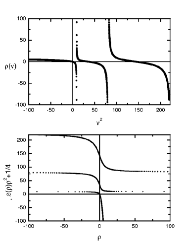
Note that the function $\rho(\nu)$, Eq.(18), is a real function if, and only if, $\nu$ takes on values along the imaginary or the real axis, see Fig. 2. It can be seen that the pseudo-Sturmian function defined in Eq.(9) coincides, apart from normalization constants, with the lowest adiabatic function $B_{0}(\theta;R^{\prime})$ when $\nu=q_{0}$ is an imaginary number and $\rho(\nu)=R^{\prime}(q_{0})$. Also, if $\nu=q_{\kappa}$ are in the real intervals $\left(3+\left[\kappa-6\right],9+\left[\kappa-6\right]\right)$ with $\kappa=6,12,...$, then $\rho(\nu)=R^{\prime}(q_{\kappa})$ and the pseudo-Sturmian functions become equal, except for the normalization constants, to the adiabatic eigenfunctions $B_{\kappa}(\theta;R^{\prime})$.

Thus, in the case of the example considered in this paper, that is $E<0$ and the $2+1$ system, the integral Eq.(12), along the imaginary axis in the complex $\nu$ plane, can be written in terms of the lowest adiabatic function as

$$\Psi(R,\theta)=\int_{\varsigma}d\nu A(\nu)B_{0}\left(\theta;R^{\prime}(\nu)\right)Z_{\nu}(KR),$$ (40)

where $\nu$ runs from $-i\infty$ to $i\infty$ . The most important contribution of the adiabatic functions to the integral, at large $R$, comes from the lines $\theta=\theta_{j}$, where two of the particles are joined. When these adiabatic functions are multiplied by the appropriate Bessels functions, their linear combination (Eq. (40)) should have the correct asymptotic behaviour, and will represent a two-body bound system in the colliding with a third particle.

Figure 2: Plot of the pseudo-Sturmian eigenvalue $\rho(\nu)$. In (a) we plot $\rho(\nu)$ as a function of $\nu^{2}$. In (b) the plot of (a) is rotated and flipped to give $\nu^{2}$ as a function of $\rho.$ For $\rho$ positive, $\nu^{2}=\Lambda(\rho)\rho^{2}+\frac{1}{4}$.
Refer to caption

Conclusions and Outlook

We have shown that the integral representation approach within the hyperspherical context, when applied to McGuireโ€™s model, offers a reliable tool to study the collisional dynamics of the 3-body system. We have obtained several interesting results, namely:

-An exact solution to the corresponding Schrรถdinger equation.

-A closed form for the angular basis for this system, the pseudo-Sturmian functions.

-A recurrence relation for the coefficients, in the expansion of the wave function in terms of the free-particle basis.

-The S-matrix, obtained directly from the solution of the recurrence relation.

-The relation of the present approach to the traditional adiabatic approach.

-The relation of the present solution to the known plane wave exact solution.

The simplicity of the approach as compared with the adiabatic one, promises to be very useful in extending it to more complicated situations, like the system with different masses and systems with more particles, currently under research, or systems in three dimensions modeled by ZRP potentials. In the last case, the method can be applied to a wide kind of systems to obtain asymptotic solutions which can be matched to solutions obtained with methods like the R-matrix one, simplifying substantially the calculations.

Acknowledgments

Oak Ridge National Laboratory, is managed by UT-Battelle, LLC under contract number DE-AC05-00OR22725. Support by the National Science Foundation under grant number PHY997206 is gratefully acknowledged. AAT thanks to CONACyT, project 4877-E for partial support and gratefully acknowledges the financial support from the National Science Foundation under grant number PHY997206 together with the hospitality of the University of Tennessee. SYL also thanks the University for making possible a visit. One of us, G.G. thanks the support under the PICT Nro. 0306249 of the ANPCyT.


APPENDIX A: Pseudo-Sturmian Functions

Fixing $\nu$, the general solution for the eigenvalue equation

$$\left[\frac{\partial^{2}}{\partial\theta^{2}}+\nu^{2}\right]\varphi(\theta)=\left[\rho\left(\nu\right)\frac{\pi c}{3}\sum_{j=0}^{5}\delta\left(\theta-\theta_{j}\right)\right]\varphi(\theta),$$ (41)

with $\theta_{j}=\left(2j+1\right)\pi/6$, can be written as the free angular wave solution $\varphi(\theta)=D_{\nu}\cos\left[\nu\left(\theta-\gamma_{j}\right)\right],\;j=0,1,...,5,$ provided that it be continuous through the boundary lines $\theta=\theta_{j}$ , that is,

$$\cos\left[\nu\left(\theta_{j}-\gamma_{j+1}\right)\right]=\cos\left[\nu\left(\theta_{j}-\gamma_{j}\right)\right],$$ (42)

and satisfies the boundary conditions

$\displaystyle\lim_{\zeta\rightarrow 0}$ $\displaystyle\int_{\theta_{j}-\zeta}^{\theta_{j}+\zeta}\left\{d\theta\left[\frac{\partial^{2}}{\partial\theta^{2}}+\nu^{2}\right]\varphi(\theta)\right.$ (43)
$\displaystyle\left.\left.-\left[\rho\left(\nu\right)\frac{\pi c}{3}\sum_{l=0}^{5}\delta\left(\theta-\theta_{l}\right)\right]\varphi(\theta)\right\}=0,\right.\;\;$

with $j=0,1,...,5\leavevmode\nobreak$ . $D_{\nu}$, which does not depend on $j$ for the symmetric solution, determined by normalizing the wave function[18]. The requirement of continuity leads to the conditions $\gamma_{j}+\gamma_{j+1}=2\theta_{j}=\left(j+\left[j+1\right]\right)\pi/3$ or to $\gamma_{j-1}=\gamma_{j}$. The second condition does not satisfy (43) so we shall use the first one, which can be written as $\gamma_{j}=j\;\pi/3$. Now to focus on Eq.( 43). Continuity implies that the integral of the second term gives zero. For each $j$, the first and the third terms give

$\displaystyle\lim_{\zeta\rightarrow 0}$ $\displaystyle\left(\frac{\partial}{\partial\theta}\left(\cos\nu\left[\theta-\gamma_{j+1}\right]\right)_{\theta=\theta_{j}+\varsigma}\right.$ (44)
$\displaystyle-\left.\frac{\partial}{\partial\theta}\left(\cos\nu\left[\theta-\gamma_{j}\right]\right)_{\theta=\theta_{j}-\varsigma}\right)$
$\displaystyle-\rho\left(\nu\right)\frac{\pi c}{3}\cos\nu\left[\theta_{j}-\gamma_{j}\right]=0.$

If we select a symmetric solution, then

$$-\frac{\partial}{\partial\theta}\cos\left(\nu\left[\theta_{j}+\varsigma-\gamma_{j+1}\right]\right)=\frac{\partial}{\partial\theta}\cos\left(\nu\left[\theta_{j}-\varsigma-\gamma_{j}\right]\right),$$ (45)

and taking the limit in Eq.(44), we obtain the desired form of the boundary condition

$$\lim_{\theta^{-}\rightarrow\theta_{j}}\frac{1}{\rho\left(\nu\right)\cos\left(\nu\left[\theta-\gamma_{j}\right]\right)}\frac{\partial}{\partial\theta}\cos\left(\nu\left[\theta-\gamma_{j}\right]\right)=-\frac{\pi c}{6},$$ (46)

where $\;j=0,1,...,5$. Calculating the derivative and the limit in Eq. (46) yields

$$\frac{6}{\pi c}v\tan\nu\pi/6=\rho\left(\nu\right).$$ (47)

We conclude that $\cos\left[\nu\left(\theta-j\pi/3\right)\right],\;j=0,1,...,5$, satisfies Eq.(41), provided that $\rho\left(\nu\right)$ satisfies Eq.(47).


APPENDIX B: Derivation of the plane wave representation in terms of cartesian coordiantes

For the $2+1$ system, and aside from an ultimate normalization, the incoming wave function from Eq.(31) can be written in terms of cartesian coordinates, as

$\displaystyle\psi^{i}$ $\displaystyle=$ $\displaystyle\exp\left\{\frac{\pi c}{6}\left(\frac{x_{1}-x_{2}}{\sqrt{2}}\cos\left[\left(j-1\right)\frac{\pi}{3}\right]\right.\right.$ (48)
$\displaystyle+\left.\frac{x_{1}+x_{2}-2x_{3}}{\sqrt{6}}\sin\left[\left(j-1\right)\frac{\pi}{3}\right]\right)$
$\displaystyle-ik\left(\frac{x_{1}+x_{2}-2x_{3}}{\sqrt{6}}\cos\left[\left(j-1\right)\frac{\pi}{3}\right]\right.$
$\displaystyle-\left.\left.\frac{x_{1}-x_{2}}{\sqrt{2}}\sin\left[-\left(j-1\right)\frac{\pi}{3}\right]\right)\right\}$
$\displaystyle+\exp\left\{-\frac{\pi c}{6}\left(\frac{x_{1}-x_{2}}{\sqrt{2}}\cos\left[\left(j+1\right)\frac{\pi}{3}\right]\right.\right.$
$\displaystyle+\left.\frac{x_{1}+x_{2}-2x_{3}}{\sqrt{6}}\sin\left[\left(j+1\right)\frac{\pi}{3}\right]\right)$
$\displaystyle-ik\left(\frac{x_{1}+x_{2}-2x_{3}}{\sqrt{6}}\cos\left[\left(j+1\right)\frac{\pi}{3}\right]\right.$
$\displaystyle-\left.\left.\frac{x_{1}-x_{2}}{\sqrt{2}}\sin\left[-\left(j+1\right)\frac{\pi}{3}\right]\right)\right\}$

Evaluating the trigonometric functions for $j=0$ in the above expression, the argument of the first exponential function takes the form

$\displaystyle i\left[\right.$ $\displaystyle-$ $\displaystyle\frac{2}{\sqrt{6}}k\;x_{1}+\left(-i\frac{\pi c}{6\sqrt{2}}+i\frac{1}{\sqrt{6}}k\right)\;x_{2}$ (49)
$\displaystyle+$ $\displaystyle\left.\left(i\frac{\pi c}{6\sqrt{2}}+i\frac{1}{\sqrt{6}}k\right)\;x_{3}.\right]$

By labeling the particle wave numbers as in [17],

$\displaystyle k_{1}$ $\displaystyle=$ $\displaystyle i\frac{\pi c}{6\sqrt{2}}-\frac{1}{\sqrt{6}}k,$
$\displaystyle k_{2}$ $\displaystyle=$ $\displaystyle-i\frac{\pi c}{6\sqrt{2}}-\frac{1}{\sqrt{6}}k,$
$\displaystyle k_{3}$ $\displaystyle=$ $\displaystyle\sqrt{\frac{2}{3}}k,$ (50)

the incoming wave takes the form

$\displaystyle\psi^{i}$ $\displaystyle=$ $\displaystyle\exp\left\{-i\left(k_{3}x_{1}+k_{2}x_{2}+k_{1}x_{3}\right)\right\}_{j=0}$
$\displaystyle+$ $\displaystyle\exp\left\{i\left(k_{2}x_{1}+k_{3}x_{2}+k_{1}x_{3}\right)\right\}_{j=0}$

The outgoing wave for $j=0$ can be obtained from the incoming one by substituting $k$ by $-k$, which in turns means interchanging $k_{1}\leftrightharpoons k_{2}$ and inverting the sign of the whole argument within all exponentials, that is,

$\displaystyle\mathcal{S}$ $\displaystyle\left[\exp\left\{-i\left(k_{1}x_{1}+k_{3}x_{2}+k_{2}x_{3}\right)\right\}_{j=0}\right.$
$\displaystyle+$ $\displaystyle\left.\exp\left\{i\left(k_{3}x_{1}+k_{1}x_{2}+k_{2}x_{3}\right)\right\}_{j=0}\right].$

The wave associated to the factor $\mathcal{S}_{3}$ can be written as

$\begin{array}[]{cc}exp&\left\{-i\left(k_{1}x_{1}+k_{2}x_{2}+k_{3}x_{3}\right)\right\}_{j=0}\\ +&\left.\exp\left\{i\left(k_{2}x_{1}+k_{1}x_{2}+k_{3}x_{3}\right)\right\}_{j=0}\right].\end{array}$

The above results correspond to the sector $j=0$ in the $(\rho,\theta)$ plane, in which the order of particles is given by $x_{2}<x_{3}<x_{1}$. The waves in different sectors can be obtained by the appropriate permutation of the set of coordinates $\left\{x_{1},x_{2},x_{3}\right\}$. The completely symmetric wave plane may then be written as

$\displaystyle\psi=\Sigma_{p}$ $\displaystyle\left[\left\{\exp\left[-i\left(k_{3}x_{1}+k_{2}x_{2}+k_{1}x_{3}\right)\right]_{j=j_{p}}\right.\right.$
$\displaystyle+\left.\exp\left[i\left(k_{2}x_{1}+k_{3}x_{2}+k_{1}x_{3}\right)\right]_{j=j_{p}}\right\}$
$\displaystyle+\mathcal{S}(p)$ $\displaystyle\left\{\exp\left[-i\left(k_{1}x_{1}+k_{3}x_{2}+k_{2}x_{3}\right)\right]_{j=j_{p}}\right.$
$\displaystyle\left.+\exp\left[i\left(k_{3}x_{1}+k_{1}x_{2}+k_{2}x_{3}\right)\right]_{j=j_{p}}\right\}$
$\displaystyle+\mathcal{S}_{3}(p)$ $\displaystyle\left\{\exp\left[-i\left(k_{1}x_{1}+k_{2}x_{2}+k_{3}x_{3}\right)\right]_{j=j_{p}}\right.$ (51)
$\displaystyle+\left.\left.\exp\left[i\left(k_{2}x_{1}+k_{1}x_{2}+k_{3}x_{3}\right)\right]_{j=j_{p}}\right\}\right]$

where the sum runs over all permutations of the set $\left\{x_{1},x_{2},x_{3}\right\}$.

References

  • [1] XVIIth European Conference on Few-Body Problems in Physics. Conference Handbook. Ed.: A. Stadler et al. Evora 2000.
  • [2] E. Nielsen and J. H. Macek, Phys. Rev. Lett 83, 1566 (1999).
  • [3] S. Inouye, M. R. Andrews, K Stenger, H.J. Miesner, D. M. Stamper-Kurn and W. Ketterle, Nature (London) 392, 151 (1998).
  • [4] A. J. Moerdijk, H. M. J. M. Boesten and B. J. Verhaar, Phys. Rev. A 53, R916 (1996).
  • [5] B. D. Esry, C. H.. Greene, Y. Zhou and C. D. Lin, J. Phys. B 29, L51 (1996).
  • [6] P. O. Fedichev, M. W. Reynolds and G. V. Shlyapnikov, Phys. Rev. Lett. 77, 2921 (1996).
  • [7] Yu. N. Demkov and V. N. Ostrovsky, Zero-Range Potentials and Their Applications in Atomic Physics. Plenum Press, NY, 1988.
  • [8] G. Gasaneo and J. H Macek, Jour. Phys. B 35 2239-2250 (2002).
  • [9] G. Gasaneo, S. Yu. Ovchinnikov and J. H. Macek, Phys. Rev. A submitted (2002).
  • [10] J. B. McGuire, J. Math. Phys. 5, (1964) 622.
  • [11] C. N. Yang, Phys. Rev. Lett. 19, 1312 (1967); C. N. Yang, Phys. Rev. 168, 1920 (1968).
  • [12] H. A. Bethe, Z. Phys. 71, (1931) 205.
  • [13] L. R. Dodd, J. Math. Phys. 11, (1970) 207; H. B. Thacker, Phys. Rev. D 11, (1975) 838; A. Amaya-Tapia, S.Y. Larsen and J. Popiel, Few-Body Sys. 23, (1997) 87; S. I. Vinitsky, S. Y. Larsen, D. V. Pavlov, D. V. Proskurin. Phys. At. Nucl. 64, 27 (2001); O. Chuluunbaatar, A. A. Gusev, S. Y. Larsen, S. I. Vinitsky. J. Phys. A35, L513 (2002)
  • [14] L. H. Thomas, Phys. Rev. 47, 903 (1935).
  • [15] G. Gasaneo, S. Yu. Ovchinnikov and J. H. Macek, Jour. of Phys. A34, (2001) 8941.
  • [16] I. S. Gradshteyn and I. M. Ryzhik, Table of Integrals, Series and Products. Academic Press, NY, 1965, p.773.
  • [17] A. Amaya-Tapia, S.Y. Larsen and J. Popiel, Few-Body Sys. 23, (1997) 87; W. Gibson, S. Y. Larsen and J. J. Popiel, Phys. Rev. A 35 (1987) 4919.
  • [18] S.Y. Larsen, in Few Body Methods: Principles and Applications. T. K. Lim, C. G. Bao, D. P. Hou and H. S. Huber, eds. p. 467, Singapore, World-Scientific 1986.