The period of a classical oscillator

Abstract

We develop a simple method to obtain approximate analytical expressions for the period of a particle moving in a given potential. The method is inspired to the Linear Delta Expansion (LDE) and it is applied to a large class of potentials. Precise formulas for the period are obtained.

In this letter we consider the problem of calculating the period of a unit mass moving in a potential $V(x)$. Although it is possible to solve this problem analytically only in a few cases, depending upon the form of the potential, several methods to find approximate results have been devised in the past. Many of the techniques that are used to solve this kind of problems are based on a perturbative expansion in some small parameter that appears in the equations of motion. This is the case of the Lindstedt-Poincaré method and of the multiple-scale method. Unfortunately the validity of these approaches is restricted to the domain of weak couplings and the series obtained rapidly diverge when larger couplings are considered. Recently, one of the authors and collaborators devised a non-perturbative version of the Lindstedt-Poincaré method, based on the ideas of the Linear Delta Expansion (LDE)lde , which allows to obtain very accurate results in a wide class of non linear problemsAA1:03 ; AA2:03 ; AM:04 . In this letter we propose a different method, also inspired by the LDE, whose application is much simpler and for which convergence to the exact result can be proven.

Let us describe the method in detail. We consider a unit mass moving in a potential $V(x)$. The total energy $E=\frac{\dot{x}^{2}}{2}+V(x)$ is conserved during the motion. The exact period of the oscillations will be given by:

$$T=\int_{x_{-}}^{x_{+}}\frac{\sqrt{2}}{\sqrt{E-V(x)}}dx,$$ (1)

where $x_{\pm}$ are the inversion points, obtained by solving the equation $E=V(x_{\pm})$.

Only in few cases it is possible to evaluate the integral (1) analytically. In the spirit of the Linear Delta Expansion (LDE) we interpolate the full potential $V(x)$ with a solvable one $V_{0}(x)$ defined as $V_{\delta}(x)=V_{0}(x)+\delta\ (V(x)-V_{0}(x))$.

We want to perform this interpolation without moving the inversion points; for this reason we ask that $x_{\pm}$ be the inversion points also of the potential $V_{0}(x)$. As a result, the energy $E_{0}$ that the particle would possess if it was moving only in the potential $V_{0}(x)$ will be given by $E_{0}=V_{0}(x_{\pm})$.

We are now in position to rewrite eq. (1) as

$$T_{\delta}=\\ \int_{x_{-}}^{x_{+}}\frac{\sqrt{2}}{\sqrt{E_{0}-V_{0}(x)+\delta\big{[}E-E_{0}-V(x)+V_{0}(x)\big{]}}}dx.$$ (2)

We notice that Eq. (2) reduces to Eq. (1) for $\delta=1$; for $\delta=0$ this formula yields the period of oscillation between the points $x_{\pm}$ in the potential $V_{0}(x)$. We will treat the term proportional to $\delta$ as a perturbation and expand in powers of $\delta$. Since $V_{0}(x)$ depends upon one or more arbitrary parameters (which we will indicate with $\lambda$) a residual dependence upon these parameters shows up in the period when the expansion is carried out to a finite order. In order to eliminate such unnatural dependence we impose the Principle of Minimal Sensitivity (PMS) Ste81 by requiring that

$$\frac{\partial T}{\partial\lambda}=0.$$

Finally, we can write explicitly the period by performing an expansion in $\delta$ and obtain

$$T_{\delta} = \int_{x_{-}}^{x_{+}}\frac{\sqrt{2}}{\sqrt{E_{0}-V_{0}(x)}}\ \frac{dx}{\sqrt{1+\delta\ \Delta(x)}}$$ (3)

$$= \int_{x_{-}}^{x_{+}}\frac{\sqrt{2}}{\sqrt{E_{0}-V_{0}(x)}}$$

$$\times\sum_{n=0}^{\infty}\frac{(2n-1)!!}{n!2^{n}}(-1)^{n}\delta^{n}\left[\Delta(x)\right]^{n}dx,$$

where

$$\Delta(x)=\frac{E-E_{0}-V(x)+V_{0}(x)}{E_{0}-V_{0}(x)}.$$ (4)

$T_{\delta}$ can be written as

$$T_{\delta}=\sum_{n=0}^{\infty}\frac{(2n-1)!!}{n!\ 2^{n}}(-1)^{n}\delta^{n}\int_{x_{-}}^{x_{+}}\frac{\sqrt{2}\ \big{(}\Delta(x)\big{)}^{n}}{\sqrt{E_{0}-V_{0}(x)}}dx$$ (5)

provided that the series in Eq. (3) converges uniformly, which is the case if $|\Delta(x)|<1$ for every $x$, $x_{-}\leq x\leq x_{+}$.

We now apply Eq. (5) to a few cases. We start with the Duffing oscillator, which corresponds to the potential $V(x)=\frac{1}{2}\ x^{2}+\frac{\mu}{4}\ x^{4}$. Although the period of the Duffing oscillator can be calculated explicitly in terms of elliptic functions, we use this example to illustrate our method and to prove its efficiency.

We choose the interpolating potential to be $V_{0}(x)=\frac{1+\lambda^{2}}{2}\ x^{2}$ and obtain

$$\Delta(x)=\frac{2}{1+\lambda^{2}}\ \left[\frac{\mu}{4}\ (A^{2}+x^{2})-\frac{\lambda^{2}}{2}\right]\ .$$

Hence the series in Eq. (5) converges to the exact period for $\lambda>\lambda_{0}\equiv\sqrt{\frac{\mu A^{2}}{2}}\ \sqrt{1-\frac{1}{\mu A^{2}}}$, since $|\Delta(x)|<1$ uniformly for such values of $\lambda$ and $|x|\leq A$.

The period of the Duffing oscillator calculated to first order using (5) is then

$$T^{(0)}_{\delta}+\delta\ T^{(1)}_{\delta}=\\ \frac{2\pi}{\sqrt{1+\lambda^{2}}}\left\{1-\frac{\delta}{1+\lambda^{2}}\ \left[\frac{3}{8}\mu A^{2}-\frac{\lambda^{2}}{2}\right]\right\}$$

By setting $\delta=1$ and applying the PMS we obtain the optimal value of $\lambda$, $\lambda_{PMS}=\frac{\sqrt{3\mu}}{2}A$, which remarkably coincides with the one obtained in AA1:03 by using the LPLDE method to third order. The period corresponding to the optimal $\lambda$ is

$$T_{PMS}=\frac{4\pi}{\sqrt{4+3\mu A^{2}}},$$

which provides an error less than $2.2\%$ to the exact period for any value of $\mu$ and $A$.

It is useful to compare this result with the one in He03 , which differs from our result only for a numerical factor under the square root. The result of He03 yields a much larger error ($16\%$) over the period. This is expected, since our first order formula complies with the PMS.

Let us now come to the issue of convergence: since $\lambda_{PMS}>\lambda_{0}$ we can write

$$T_{\delta}=\sum_{n=0}^{\infty}\delta^{n}T_{\delta}^{(n)},$$ (6)

where

$$T_{\delta}^{(n)}=\frac{(-1)^{n}\pi(2n-1)!!}{2^{2n-1}n!\sqrt{1+\lambda^{2}}}\left(\frac{A^{2}\mu-2\lambda^{2}}{1+\lambda^{2}}\right)^{n}\times\\ {}_{2}F_{1}\left(\frac{1}{2},-n,1,\frac{A^{2}\mu}{2\lambda^{2}-A^{2}\mu}\right).$$ (7)

${}_{2}F_{1}$ is the hypergeometric function. Since Eq. (7) is essentially a power series, it converges exponentially to the exact result, which is precisely what we observe in Figure 1, where we plot the error $\Xi\equiv\left[\frac{T_{PMS}-T_{exact}}{T_{exact}}\right]\ \times 100$ for three different values of the parameter $\lambda$ as a function of the order in the expansion. $T_{exact}$ is the exact period of the Duffing oscillator. Corresponding to the optimal value of the parameter, $\lambda_{PMS}=\sqrt{3\ \mu A^{2}}/2$, the rate of convergence is maximal.

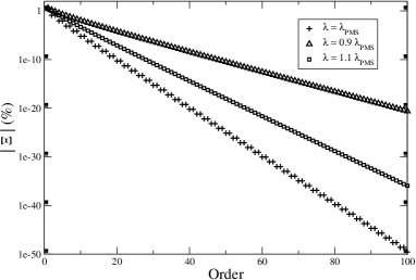
Figure 1: Error over the period (in absolute value), defined as $\Xi\equiv\left[\frac{T_{PMS}-T_{exact}}{T_{exact}}\right]\ \times 100$, for $A=10$ and $\mu=1$ as a function of the order. The three sets are obtained by using the optimal value $\lambda_{PMS}=\sqrt{3\ \mu A^{2}}/2$ (plus), a value $\lambda=0.9\ \lambda_{PMS}$ (triangle) and $\lambda=1.1\ \lambda_{PMS}$ (square).

We now consider the general anharmonic potential $V(x)=\frac{1}{2}\ x^{2}+\rho\ \frac{x^{2N}}{2N}$ and obtain

$$\Delta(x)=\frac{2}{1+\lambda^{2}}\left[\frac{\rho}{2N}\frac{A^{2N}-x^{2N}}{A^{2}-x^{2}}-\frac{\lambda^{2}}{2}\right].$$

To first order, Eq. (5) gives

$$T^{(0)}_{\delta}+\delta T^{(1)}_{\delta}=\frac{2\pi}{\sqrt{1+\lambda^{2}}}\ \times\\ \bigg{\{}1+\frac{\delta}{1+\lambda^{2}}\Big{(}-\rho\ A^{2(N-1)}\frac{\Gamma(N+1/2)}{\sqrt{\pi}\Gamma(N+1)}+\frac{\lambda^{2}}{2}\Big{)}\bigg{\}},$$

in which case the optimal value of $\lambda$ is given by:

$$\lambda_{PMS}=\sqrt{\frac{2\rho\Gamma(N+1/2)}{\sqrt{\pi}\Gamma(N+1)}}A^{N-1}.$$

This time, these values of $\lambda$ do not coincide with the ones obtained with the LPLDE method to third order for $N=3$ and $N=4$ AM:04 . With such $\lambda$ one obtains the expression

$$T_{PMS}=\frac{2\pi}{\sqrt{1+\displaystyle\frac{2\rho A^{2(N-1)}\Gamma(N+1/2)}{\sqrt{\pi}\Gamma(N+1)}}}.$$ (8)

We have tested Eq. (8) for moderate values of $\rho$ and $A$ and seen that it provides a very good approximation to the exact period, even when the anharmonicity exponent $N$ gets very large.

We consider now the nonlinear pendulum, whose potential is given by $V(\theta)=1-\cos\theta$. By choosing the interpolating potential to be $V_{0}(\theta)=\frac{1+\lambda^{2}}{2}\theta^{2}$ we obtain

$$\Delta(\theta)=-\frac{2}{1+\lambda^{2}}\frac{\cos\Theta-\cos\theta}{\Theta^{2}-\theta^{2}}-1,$$

where $\Theta$ is the amplitude of the oscillations. To first order our formula yields

$$T_{\delta}=\frac{2\pi}{\sqrt{1+\lambda^{2}}}\Big{(}1+\frac{\delta}{2}\Big{)}-\frac{2\pi\delta}{(1+\lambda^{2})^{3/2}}\frac{J_{1}(\Theta)}{\Theta},$$

where $J_{1}$ is the Bessel function of the first kind of order 1. The optimal value of $\lambda$ in this case is given by

$$\lambda_{PMS}=\sqrt{\frac{2J_{1}(\Theta)}{\Theta}-1}$$

and the period to first order is then

$$T_{PMS}=\pi\sqrt{\frac{2\ \Theta}{J_{1}(\Theta)}}.$$ (9)

Eq. (9) provides an excellent approximation to the exact period over a wide range of amplitudes.

We now apply our expansion to two problems in General Relativity: the calculation of the deflection of the light by the Sun and the calculation of the precession of a planet orbiting around the Sun. We use the notation of Weinberg Weinberg :

$$B(r)=A^{-1}(r)=1-\frac{2GM}{r}.$$

The angle of deflection of the light by the Sun is given by the expression

$$\Delta\phi=2\int_{r_{0}}^{\infty}\sqrt{A(r)}\left[\left(\frac{r}{r_{0}}\right)^{2}\frac{B(r_{0})}{B(r)}-1\right]^{-1/2}\frac{dr}{r}-\pi$$

where $r_{0}$ is the closest approach.

With the change of variable $z=1/r$ we obtain

$$\Delta\phi=2\ r_{0}^{3/2}\int_{0}^{1/r_{0}}\frac{dz}{\sqrt{r_{0}-r_{0}^{3}z^{2}-2GM(1-r_{0}^{3}z^{2})}}-\pi,$$

which is exactly in the form required by our method. We introduce the potential $V_{0}(z)=(r_{0}^{3}-\lambda^{2})\ z^{2}$ to obtain

$$\Delta(z)=\frac{r_{0}(1-r_{0}^{2}z^{2})-2GM\ (1-r_{0}^{3}z^{3})}{(r_{0}^{3}+\lambda^{2})\left(\frac{1}{r_{0}^{2}}-z^{2}\right)}.$$

By applying our method to first order we obtain

$$\Delta\phi^{(0)}_{\delta}+\delta\Delta\phi^{(0)}_{\delta}=\\ -\pi+\frac{\pi\left(2+\displaystyle\frac{\left(2+\delta\right)\lambda^{2}}{r_{0}^{3}}\right)+\displaystyle\frac{8\delta GM}{r_{0}}}{2{\left(1+\displaystyle\frac{{\lambda}^{2}}{{{r_{0}}}^{3}}\right)}^{\frac{3}{2}}}.$$ (10)

The optimal value of the parameter $\lambda$ obtained by the PMS is given by

$$\lambda_{PMS}=2i\sqrt{\frac{2GM}{\pi}}r_{0}.$$

The deflection angle corresponding to this value of $\lambda$ reads

$$\Delta\phi_{PMS}=-\pi+\sqrt{\frac{\pi}{1-\displaystyle\frac{8GM}{r_{0}\pi}}}.$$ (11)

The surface corresponding to the closest approach for which $\Delta\phi$ diverges is known as photon sphere and for the Schwartzchild metric takes the value $r_{0}=3GM$. It is remarkable that Eq. (11), despite its simplicity, is able to predict a slightly smaller photon sphere, corresponding to $r_{0}=8GM/\pi$. Clearly, this feature is completely missed in a perturbative approach.

In Figure 2 we compare Eq. (11) with the exact numerical result, the post-post-Newtonian (PPN) result of Epstein and with the asymptotic result for very small values of $r_{0}$ (close to the photon sphere). In Figure 3 we plot the error over the deflection angle obtained by using Eq. (11) or the PPN result in a range of $r_{0}$ of practical interest. Our formula gives an error which is two orders of magnitude smaller than the one obtained with the PPN.

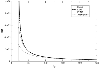
Figure 2: Deflection angle of light obtained assuming $G/c^{2}=7.425\times 10^{-30}\ m/kg$ and $M=1.97\times 10^{30}\ kg$ as function of the closest approach $r_{0}$. The solid line is the exact (numerical) result, the dashed line is obtained with Eq. (11), the dotted line is the post-post-Newtonian result of Epstein , the dot-dashed line is the asymptotic result ($r_{0}\rightarrow\infty$). The vertical line marks the location of the photon sphere, where the deflection angle diverges.

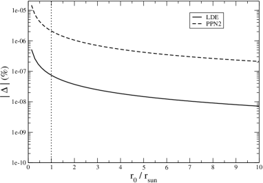
Figure 3: Absolute value of the error over the deflection angle as a function of the closest approach in units of the sun radius ($r_{sun}=6.95\times 10^{8}\ m$), assuming $G/c^{2}=7.425\times 10^{-30}\ m/kg$ and $M=1.97\times 10^{30}\ kg$. The error is defined as $\Delta\equiv\frac{\Delta\phi_{approx}-\Delta\phi_{exact}}{\Delta\phi_{exact}}$. The solid line is the error obtained with eq. (11), while the dashed line is the error obtained using the PPN approximation of Epstein . The vertical line marks the solar radius.

Finally we consider the problem of calculating the precession of the perihelion of a planet orbiting around the Sun. The angular precession is given by Weinberg

$$\Delta\theta=-2\pi-2\int_{r_{-}}^{r_{+}}\frac{\sqrt{A(r)}\ dr}{r^{2}\sqrt{\displaystyle\frac{1}{J^{2}B(r)}-\frac{E}{J^{2}}-\frac{1}{r^{2}}}}$$ (12)

where $E=\left(\frac{r_{+}^{2}}{B(r_{+})}-\frac{r_{-}^{2}}{B(r_{-})}\right)/\left(r_{+}^{2}-r_{-}^{2}\right)$ and $J^{2}=\left(\frac{1}{B(r_{+})}-\frac{1}{B(r_{-})}\right)/\left(\frac{1}{r_{+}^{2}}-\frac{1}{r_{-}^{2}}\right)$. $r_{\pm}$ are the shortest (perielia) and largest (afelia) distances from the sun. By the change of variable $z=1/r$ we can write Eq. (12) as

$$\Delta\theta=-2\int_{z_{-}}^{z_{+}}\frac{1}{\sqrt{(z_{+}-z)(z-z_{-})}}\times\\ \frac{dz}{\sqrt{(1-2GM(z+z_{-}+z_{+}))}}-2\pi,$$

where $z_{\pm}\equiv 1/r_{\mp}$.

We write

$$\Delta\theta_{\delta}=-2\int_{z_{-}}^{z_{+}}\frac{1}{\sqrt{(z_{+}-z)(z-z_{-})}}\times\\ \frac{dz}{\sqrt{(1-\lambda^{2}+\delta(-2GM(z+z_{-}+z_{+})+\lambda^{2}))}}-2\pi.$$

As usual we treat the term proportional to $\delta$ as a perturbation and expand to third order. The optimal value of $\lambda$ is obtained by using the PMS

$$\lambda_{PMS}=\sqrt{\frac{6GM}{L}},$$

and yields the precession

$$\Delta\theta=\\ \frac{\pi(3G^{2}LM^{2}+a(-4L^{2}+48GLM-147G^{2}M^{2}))}{4a(L-6GM)^{2}\sqrt{1-\displaystyle\frac{6\ G\ M}{L}}},$$ (13)

where $a$ is the semimajor axis of the ellipse, given by $a\equiv(r_{-}+r_{+})/2$, and $L$ is the semilatus rectum of the ellipse, given by $1/L=(1/r_{+}+1/r_{-})/2$.

In Figure 4 we plot the precession of the orbit calculated through the exact formula (solid line), through Eq. (13) (dashed line) and through the leading order result Weinberg $\Delta\theta_{0}=\frac{6\pi GM}{L}$ (dotted line) . Once again we find excellent agreement with the exact result.

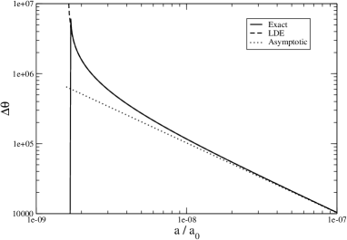
Figure 4: Precession of the orbit of a planet assuming the values $M=1.97\times 10^{30}\ kg$, $G/c^{2}=7.425\times 10^{-30}\ m/kg$ and $\varepsilon=0.2506$ (eccentricity). The scale of reference $a_{0}$ is taken to be the semimajor axis of Mercury’s orbit ($a_{0}=5.971\times 10^{10}\ m$). The solid line is the exact result, the dashed line is the result of Eq. (13) and the dotted line is the leading term in the perturbative expansion.

In conclusion, we have devised a method to calculate with high accuracy a certain class of integrals, which are very common in many physical problems. The convergence of our expansion to the exact result is easy to verify, as we have explicitly shown in one special case. Moreover the lowest order results obtained by applying our method already provide an excellent agreement with the full exact results. Work is currently in progress to apply this technique to a wider class of problems.

References

(1) A. Okopińska, Phys. Rev. D 35, 1835 (1987); A. Duncan and M. Moshe,
Phys. Lett. B 215, 352 (1988)
(2) Amore P and Aranda A,
Phys. Lett. A316 218
(3) Amore P and Aranda A,
Preprint math-ph/0303052
(4) Amore P and Montes H,
accepted for publication on Physics Letters A,
Preprint math-ph/0310060
(5) P. M. Stevenson,
Phys. Rev. D 23, 2916 (1981).
(6) J. He, Phys. Rev. Lett.90 174301 (2003)
(7) S. Weinberg, Gravitation and cosmology, J.Wiley and Sons, 1972
(8) R. Epstein and I. Shapiro, Phys. Rev. D 22, 2947 (1980);
E. Fischbach and B. Freeman, Phys. Rev. D 22, 2950 (1980)