Boundary condition at the junction

1 Introduction

Practical calculation of transport properties of quantum networks is often reduced to the scattering problem for a one-dimensional differential operator on a quantum graph, see for instance [1, 2, 3, 4, 5]. Quantum graph plays a role of a solvable model for a two-dimensional network, see [6, 7, 8]. Basic detail of the model is a star-shape element with a self-adjoint boundary condition at the node. It was commonly expected that the realistic boundary condition is defined by the angles between the wires at the node. For instance the boundary conditions for the T-junction, [1], is presented in terms of limit values of the wave-function on the wires $\left\{\psi_{i}\right\}^{3}_{i=1}:=\vec{\psi}$ and the values of the corresponding outward derivative $\left\{\psi^{\prime}_{i}\right\}^{3}_{i=1}:=\vec{\psi^{\prime}}$ at the node:

$$\beta^{-1}\psi_{1}=\psi_{2}=\psi_{3}\,,\quad\beta\psi^{\prime}_{1}+\psi^{\prime}_{2}+\psi^{\prime}_{3}=0,$$ (1)

or in the form

$$P_{0}^{\perp}\vec{\psi}=0\,,\quad P_{0}\vec{\psi}^{\prime}=0$$ (2)

with the projection

$$P_{0}=\frac{1}{\beta^{2}+2}\left(\begin{array}[]{ccc}\beta^{2}&\beta&\beta\\ \beta&1&1\\ \beta&1&1\end{array}\right).$$

The scattering matrix of such a junction is $S=I-2P_{0}$, see [1, 4, 10]. In [1] $\beta$ is interpreted as a free parameter describing the strength of coupling between the leg and the bar of the T-junction. In [11] the condition ( 2) is used for analysis of spin-dependent transmission across the quantum ring.

We derive the boundary condition (2) and similar condition for any junction from [13] and interpret the corresponding free parameters $\beta,P_{0}$.

2 Intermediate Hamiltonian

Consider one body scattering problem on the junction $\Omega$ formed by few 2-d equivalent semi-infinite wires $\Omega_{j},\,\,s=1,2,\dots$, attached to the quantum well $\Omega_{int}$ via the orthogonal bottom sections $\Gamma_{s}$. The corresponding one-body Hamiltonian for the spin-less electron is scaled, via replacement of energy $E$ by the spectral parameter $\lambda=\hbar^{-2}2m*E$, to the standard Schrödinger operator with zero conditions on the boundary $\partial\Omega$, and a constant potential in the wires $q|_{\Omega_{s}}=q_{\infty}$:

$${\cal L}\psi=-\bigtriangleup\psi+q\psi.$$ (3)

We assume, following [13], that the potential on the well is defined by the scaled constant electric field $\cal{E}$: $q|_{\Omega_{int}}=q_{int}(x)=\langle\cal{E},x\rangle,x\in\Omega_{int}$. The role of the non-perturbed Hamiltonian is played by the Schrödinger operator ${\cal L}_{out}$ on the wires with zero boundary conditions on the union $\Gamma=\cup_{s}\Gamma_{s}$ of the bottom sections, which play roles of solid walls, separating the well from the wires:

$$\psi|_{\Gamma}=0.$$ (4)

The eigenfunctions of ${\cal L}_{out}$ in the wires $\Omega_{s}:0<x_{s}=x<\infty,\,0<y_{s}=y<\delta$ are combined of running waves

$$\exp(\pm i\sqrt{\lambda-\pi^{2}l^{2}\delta^{-2}-q_{\infty}}x)\,\sqrt{2/\delta}\sin\pi ly/\delta$$

$$:=\exp(\pm i{p_{l}}x)\,\,\,e_{s}^{l}.$$

Hereafter we use on the wires the local coordinates $x,y,\,\,0<x,\infty,\,0<y<\delta$. The eigenfunctions of the operator $L_{int}$ defined by (3,4) on the quantum well $\Omega_{int}$ are standing waves. Replacement of the solid wall condition (4) by the matching condition is a strong perturbation blending the standing waves on the quantum well with the running waves in the wires. This is a perturbation on the continuous spectrum, so the convergence of the corresponding series can’t be estimated in spectral terms of self-adjoint operators. In [13] we suggested a modified analytic perturbation procedure based on introduction of an Intermediate Hamiltonian obtained via appropriate splitting, see [15] of ${\cal L}$.

Assume that the Fermi level in the vires lies in the middle of the first spectral band $2m*E_{F}\hbar^{-2}:=\lambda_{F}=\pi^{2}\delta^{-2}5/2+q_{\infty}$. In that case all branches of the continuous spectrum with thresholds $\pi^{2}l^{2}\delta^{-2}+q_{\infty},\,l\geq 2,$ are closed, that is all exponential solutions $\exp\pm i{p_{l}}x\,\,\,e_{s}^{l},\,,\,l\geq 2,$ of the homogeneous equation $-\bigtriangleup\psi+q\psi=\lambda\psi$ in the wires are exponentially decreasing. Impose, additionally to (1) the semi-transparent boundary condition on the bottom section

$$u|_{\Gamma}\bot E_{+},\,\,E_{+}=\bigvee_{s=1}^{3}e_{s}^{1},$$ (5)

This boundary condition prevents excitations from the first channel ${\cal H}_{+}=E_{+}\times L_{2}(R_{+})$ in the wires from entering into the quantum well, and, vice versa, exiting from the quantum well into the wires, but does not stop the excitations from the closed channels ${\cal H}_{-}=[\bigvee_{l>1}e_{s}^{l}]\times L_{2}(R_{+})$. The corresponding operator ${\cal L}^{F}$ is split into the orthogonal sum of the trivial operator in the open first channel ${\cal H}_{+}$

$$l^{F}u=-\frac{d^{2}u}{dx^{2}}+[q_{\infty}+\pi^{2}\delta^{-2}]u,\,\,,$$

with zero boundary condition on $\Gamma$, and the intermediate Hamiltonian $L^{F}$ in the orthogonal complement ${\cal H}^{F}=\left\{L_{2}(\Omega)\ominus{\cal H}_{+}\right\}$. The spectrum $\sigma_{a}(l^{F})$ coincides with the first spectral branch and the continuous spectrum $\sigma_{a}(l^{F})$ of $L^{F}$ is $[4\pi^{2}/\delta^{2}+q_{\infty},\,\infty)$.

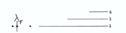
Figure 1: Spectrum of $L^{F}$

There is a finite number of eigenvalues of $L^{F}$ situated inside the first spectral band $\Delta_{1}=[\pi^{2}/\delta^{2}+q_{\infty},\,4\pi^{2}/\delta^{2}+q_{\infty}]$ and a countable number of embedded eigenvalues of $\lambda^{F}_{r}\in\sigma_{a}(L^{F})$ accumulating at infinity.

3 Scattering matrix via Intermediate DN map

Usually the Scattering matrix on the quantum network is obtained via matching exponential solutions in the wires to the solutions of the homogeneous Schrödinger equation inside the vertex domain,see, for instance [16]. This approach requires solving an infinite algebraic system. We consider the boundary problem for the intermediate equation:

$$-\bigtriangleup\psi+q\psi=\lambda\psi,\,\psi\in L_{2}(\omega),$$

$$\psi|_{\Gamma}=\psi_{\Gamma}\in E_{+},\,\,\Im\lambda\neq 0.$$ (6)

The solution $\psi$ exists for all complex $\lambda$ and has normal limit values on the continuous spectrum. We introduce the Dirichlet-to-Neumann map of the intermediate Hamiltonian (DN-map) as

$${\cal DN}^{F}:\psi_{\Gamma}\longrightarrow P_{+}\frac{\partial\psi}{\partial n}\psi_{\Gamma},$$ (7)

with $P_{+}:=P_{E_{+}}$. It is a $3\times 3$ matrix-function which is obtained via differentiation with respect to exterior normal of the resolvent of the intermediate operator restricted onto $\Omega_{int}$ and framed by $P_{+}$. It has the kernel:

$${\cal DN}^{F}(y,\eta)=-P_{+}\frac{\partial^{2}G_{\lambda}(y,\eta)}{\partial n_{y}\partial n_{\eta}}P_{+}.$$

It has the spectral representation on the complement of the spectrum of $\sigma(L^{F})$

$${\cal DN}^{F}(\lambda)=\sum_{r}\frac{P_{+}\frac{\partial\phi_{r}(\xi)}{\partial n}\rangle\,\langle P_{+}\frac{\partial\phi_{{}_{r}}(\xi^{\prime})}{\partial n}}{\lambda-\lambda_{r}}+{\cal K}^{F}(\lambda),$$ (8)

where the summation is extended over discrete spectrum of $L^{F}$ and ${\cal K}^{F}(\lambda)$ contains an integral over the continuous spectrum of $L^{F}$. The scattering matrix of ${\cal L}$ is obtained via matching of the scattering Ansatz on the open channel in wires with $p=p_{1}$:

$$e^{{}^{ip\xi}}e_{{}_{+}}+e^{{}^{-ip\xi}}S(p)e_{{}_{+}}$$ (9)

to the limit values on the spectrum, $\Im\lambda\to 0$ of the solution of the above intermediate boundary problem (7):

$$ip\left[e_{{}_{+}}-S(p)e_{{}_{+}}\right]={\cal DN}^{F}(\lambda)\,\left[e_{{}_{+}}+S(p)e_{{}_{+}}\right].$$

Solving this equation we obtain, see [13], the formula for the scattering matrix of the operator ${\cal L}$ on the first spectral band $\Delta=[\pi^{2}/\delta^{2}+q_{infty},\,4\,\pi^{2}/\delta^{2}+q_{infty},\,]$ in terms of ${\cal L}^{F}$ by the formula

$$S(p)=\frac{{\cal DN}^{F}(\lambda)+ipP_{+}}{-{\cal DN}^{F}(\lambda)+ipP_{+}}.$$ (10)

The DN-map ${\cal DN}^{{}^{F}}$ of the intermediate Hamiltonian $L_{{}_{F}}$ is connected with the standard [12] DN-map $\Lambda$ of the operator $L_{int}$ on the quantum well $\Omega$ by the formula

$${\cal DN}^{{}^{F}}=P_{+}{\cal DN}P_{+}-P_{+}{\cal DN}P_{{}_{-}}\,\,{\bf D}^{-1}P_{-}{\cal DN}P_{+}.$$ (11)

Here

$${\bf D}=P_{-}{\cal DN}P_{-}-\,K_{{}_{-}},\,\,$$

with

$$K_{-}=-\oplus\sum_{l>1}p_{l}P_{l},\,|K_{-}|\geq\pi\delta^{-1}\sqrt{3/2}.$$

and $P_{-}:=\oplus\sum_{l>1}\sum_{s}e_{s}^{l}\rangle\langle e_{s}^{l}$. Near the eigenvalue $\lambda_{0}$ of $L_{int}$ the DN-map can be decomposed as

$${\cal DN}^{F}(\lambda)=\frac{\phi_{{}_{0}}\rangle\langle\phi_{{}_{0}}}{\lambda-{\lambda_{0}}}+\sum_{s\neq 0}\frac{\phi_{{}_{s}}\rangle\langle\phi_{{}_{s}}}{\lambda-{\lambda_{s}}}:=\frac{\phi_{{}_{0}}\rangle\langle\phi_{{}_{0}}}{\lambda-{\lambda_{0}}}+{\cal K}_{{0}},$$ (12)

where $\phi_{{}_{s}}=P_{{}_{-}}\frac{\partial\Phi_{{}_{s}}}{\partial n}|_{{\Gamma}},\,s=0,1,\dots$ are the boundary currents of eigenfunctions $\Phi_{{}_{s}},\,s=0,1,2\dots$ of the operator $L_{int}$, $\lambda_{{s}}$ - the corresponding eigenvalues. Spacing between the eigenvalues of $L_{int}$ is connected to the diameter $d_{int}$ of $\Omega_{int}$ as $\rho_{0}=\min_{r\neq 0}|\lambda_{0}-\lambda_{r}|=O(d_{int}^{-2}$. Due to the spectral estimate $|{\cal K}_{{0}}(\lambda_{0})|\approx\rho_{0}^{-1}$. For relatively thin networks the analytic perturbation procedure can be developed based on (11), with the small parameter $\delta/d_{int}$, to obtain ${\cal DN}^{F}$. Denote by ${\cal K}_{\pm,\pm}$ the matrix elements $P_{\pm}{\cal K}_{{0}}P_{\pm}$ with respect to the orthogonal decomposition $L_{2}(\Gamma)=E_{+}\oplus E_{-}$. If only one eigenvalue $\lambda_{0}$ of $L_{int}$ is situated of the essential spectral interval $\Delta_{T}=[\lambda^{F}-2\hbar^{2}m^{*}\kappa T,\,\lambda^{F}+2\hbar^{2}m^{*}\kappa T$, we can represent the denominator $\bf D$ of (12) near $\lambda_{0}$, with $P_{-}\phi_{0}:={\phi}^{{-}}_{0}$ with a controllable error $k$:

$${\bf D}(\lambda)=\frac{{\phi}^{{-}}_{0}\rangle\langle{\phi}^{{-}}_{0}}{{\lambda}-{\lambda_{0}}}+{{\cal K}}_{--}-K_{-}:=\frac{{\phi}^{{-}}_{0}\rangle\langle{\phi}^{{-}}_{0}}{{\lambda}-{\lambda^{0}_{0}}}+k$$

so that the whole expression (11) can be calculated via analytic perturbation procedure, since $k\approx\delta^{-1}[1+d_{int}^{-2}]>>1$:

$$\Lambda^{{}^{F}}\approx\frac{\phi_{{}_{0}}^{{}^{F}}\rangle\,\langle\phi_{0}^{{}^{F}}}{\lambda-\lambda_{0}^{F}},$$ (13)

with $\lambda_{0}^{F}={\lambda}_{0}+\langle P_{-}\phi_{0},\,k^{{}^{-1}}\,\,\,P_{-}\phi_{0}\rangle\approx\lambda_{0}$ and $\phi_{0}^{F}=P_{+}\phi_{0}-{\cal K}_{{+-}}k^{{-1}}\,\,P_{-}\phi_{0}\approx P_{+}\phi_{0}$. For low temperature only electrons with energy close to Fermi level $E_{F}$ contribute to transport phenomena. Hence ${\cal DN}^{F}$ may be substituted by the single resonance term $\frac{P_{0}{\phi}^{-}_{{0}}\rangle\,\langle P_{0}{\phi}_{{}_{0}}}{\lambda_{0}-\lambda},$ thus resulting in the approximate expression for the scattering matrix on $\Delta_{T}$ :

$$S_{approx}(\lambda)=\frac{ipP_{0}-\frac{{P_{0}\phi}_{{0}}\rangle\,\langle{P_{0}\phi}_{{0}}}{\lambda_{0}-\lambda}}{ipP_{0}+\frac{P_{0}{\phi}_{{0}}\rangle\,\langle P_{0}{\phi}_{{0}}}{\lambda_{0}-\lambda}},$$ (14)

see [13] and more details in [17].

4 Boundary condition at the junction

The approximate scattering matrix can be obtained from the energy-dependent boundary condition at the vertex imposed onto the scattering Ansatz (9) in the wires:

$$ip[I-S_{approx}(\lambda)]\vec{\psi}=[I+S_{approx}(\lambda)]\vec{\psi}^{\prime}.$$ (15)

The polar terms in the numerator and in the denominator of (14) have the dimension $cm^{-1}$ and can be represented via the relevant one-dimensional orthogonal projection $P_{{}_{0}}:=\vec{e}_{{}_{0}}\rangle\,\langle\vec{e}_{{}_{0}}$ with $\vec{e}_{{}_{0}}:=(e_{0}^{1},e_{0}^{2},\dots e_{0}^{n})=\parallel\vec{\phi}_{{}_{0}}\parallel^{-1}\vec{\phi}_{{}_{0}}:=\alpha^{-1}\vec{\phi}_{{}_{0}}$. Then $\vec{\phi}_{{}_{0}}\rangle\,\langle\vec{\phi}_{{}_{0}}=\alpha^{{}^{2}}P_{{}_{0}}$. Denoting by $P^{{}^{\bot}}_{{}_{0}}$ the complementary projection $I-P^{{}^{\bot}}_{{}_{0}}$ in $L_{2}(\Gamma)$, we obtain

$$S_{approx}(\lambda)=P^{{}^{\bot}}_{{}_{0}}+\left[\frac{ip(\lambda-\lambda_{0})+\alpha^{{}^{2}}}{ip(\lambda-\lambda_{0})-\alpha^{{}^{2}}}\right]P_{{}_{0}}$$ (16)

$$\equiv P^{{}^{\bot}}_{{}_{0}}+\Theta(\lambda)\,P_{{}_{0}}.$$

The factor $\Theta$ is close to $-1$ on the essential spectral interval $\Delta_{T}$, for low temperature $2\pi m*\sqrt{3/2}\kappa T<<\delta\alpha^{2}\hbar^{2}$. Then, in first approximation, the energy-dependent boundary condition (15) is reduced on $\Delta_{T}$ to $iP^{{\bot}}_{{0}}\psi-P_{{0}}\psi^{\prime}\approx 0$, or, due to orthogonality of $P_{{0}},P^{{\bot}}_{{0}}$, to $P^{{\bot}}_{{0}}\vec{\psi}\approx 0;\,P_{{}_{0}}\vec{\psi}^{\prime}\approx 0$. This condition coincides with the above Datta condition (1) presented in form (2). Our analysis reveals the meaning of the projection $P_{0}$: it coincides with the projection onto the one-dimensional subspace defined by the vector $P_{+}\frac{\partial\phi_{0}(\xi)}{\partial n}|_{\Gamma}$ of boundary values of the normal derivatives of the resonance eigenfunction, projected onto $E_{+}$. This formula is valid also for general junctions.

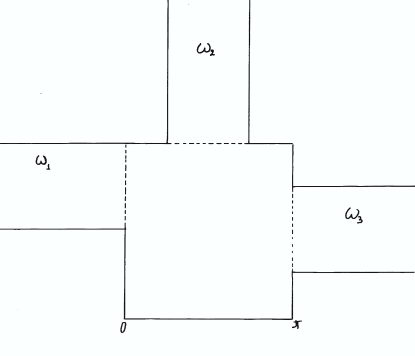
Figure 2: Simplest asymmetric T-junction

5 Example

Consider a two-dimensional quantum network constructed as a simplest asymmetric T-junction of three straight quantum wires width $\pi/2$ attached to the quantum well - the square $\Omega_{int}$ on $\xi$-plane : $0<\xi_{{}_{1}}<\pi,\,0<\xi_{{}_{2}}<\pi$. Assume that the first wire $\omega_{{1}}=\left\{-\infty<\xi_{{}_{1}}<0,\,\pi/2<\xi_{{}_{2}}<\pi\right\}$ is attached orthogonally to the left side of $\partial\Omega$ on $\Gamma_{{1}}=\left\{\xi_{{1}}=0,\,\pi/2<\xi_{{2}}<\pi\right\}$,  the second wire $\omega_{{}_{2}}=\left\{0<\xi_{{1}}<\pi/2,\,\pi<\xi_{{2}}<\infty\right\}$ is attached in the middle of the upper side, and the third wire $\omega_{{}_{3}}=\left\{\pi<\xi_{{}_{1}}<\infty,\,0<\xi_{{}_{2}}<\pi\right\}$ is attached to the middle of the right side of $\Omega_{int}$. On the constructed quantum network $\Omega=\Omega_{int}\cup\omega_{{1}}\cup\omega_{{2}}\cup\omega_{{3}}$ consider the scattering problem for Laplacian with homogeneous Dirichlet boundary condition at the boundary. The cross-section eigenfunctions in the first channel in the wires $\omega 1,\,\omega-2,\,\omega_{3}$ are :

$$e^{1}\bigg{|}_{\Gamma_{1}}=\frac{2}{\sqrt{\pi}}\sin 2\xi_{2},\,\,e^{2}\bigg{|}_{\Gamma_{2}}=\frac{2}{\sqrt{\pi}}\cos 2\xi_{1},\,\,$$

$$e^{3}\bigg{|}_{\Gamma_{3}}=\frac{2}{\sqrt{\pi}}\cos 2\xi_{2}$$

The Dirichlet Laplacian on $\Omega_{int}$ has on the first spectral band $\Delta_{1}=[4,16]$ the eigenvalues $\lambda_{{}_{0}}=5$ ,$\lambda_{1}=8$, $\lambda_{{}_{2}}=10$ and $\lambda_{{}_{3}}=13$ with eigenfunctions $\Phi_{0},\Phi_{1},\Phi_{2}.\Phi_{3}$, $\Phi_{0}=\frac{2}{\pi}\sin\xi_{1}\sin 2\xi_{2}$. The boundary currents of $\Phi_{0}$ are

$$\frac{\partial\Phi_{0}}{\partial n}\bigg{|}_{\Gamma_{1}}=-\frac{2}{\pi}\sin 2\xi_{2},\,\frac{\partial\Phi_{0}}{\partial n}\bigg{|}_{\Gamma_{2}}=-\frac{4}{\pi}\sin\xi_{1},\,$$

$$\frac{\partial\Phi_{0}}{\partial n}\bigg{|}_{\Gamma_{3}}=\frac{2}{\pi}\sin 2\xi_{2}.$$

Assume that the Fermi level of the material is situated between the first and the second thresholds of the network $4<E_{{}_{F}}<16$ close to the eigenvalue $\lambda_{0}=5\,\,cm^{{}^{-2}},\,\lambda^{F}=4.33\,\,cm^{-2}$. The electrons are supplied to the network in the first spectral band from the second wire across the bottom section $\Gamma_{2}$ and exit across $\Gamma_{1},\,\Gamma_{3}$. Due to orthogonality of the cross-section eigenfunction of the open channel to the boundary currents of the eigenfunctions $\Phi^{\prime}_{{0}},\,\Phi^{\prime}_{{3}}$ the corresponding modes are not excited. An essential link to the closed channels is supplied only by $\Phi_{{0}}$, the contribution from other eigenfunctions either vanish or are suppressed due to the factors $(\lambda_{{0}}-\lambda_{s})$ in the denominator. The link of $\Phi_{{0}}$ only to the closed channel in $\omega_{{3}}$ gives a scalar equation for the re-normalized eigenvalue $\hat{\lambda}_{{0}}$ of the intermediate Hamiltonian, since only the contribution from $\Gamma_{{}_{3}}$ is non-trivial:

$$\frac{1}{\hat{\lambda}_{0}-5}\int_{{}_{\Gamma_{{}_{3}}}}\bigg{|}P_{{}_{-}}\frac{\partial\Phi_{{}_{0}}}{\partial n}\bigg{|}^{{}^{2}}d\Gamma_{{}_{3}}+\sqrt{16-5}:={\bf D}_{{}_{-}}(\hat{\lambda}_{0})=$$

$$\sqrt{11}\,\,[0.67+\hat{\lambda}_{0}-5]$$ (17)

From this equation we obtain the resonance eigenvalue of the intermediate Hamiltonian: $\hat{\lambda}_{0}=4.33=\lambda^{{F}}$. The boundary current of the corresponding eigenfunction essentially coincides with the boundary current of the normalized resonance eigenfunction $\Phi_{{}_{0}}$ of the Dirichlet Laplacian on $\Omega_{{0}}$. The projections of the resonance boundary currents onto $E_{+}$ are

$$\phi_{0}^{1}=\int_{{\Gamma_{{1}}}}\,\frac{\partial\Phi_{{0}}}{\partial n}\bigg{|}_{{\Gamma_{{1}}}}\,e^{{1}}_{{+}}\bigg{|}_{{\Gamma_{{1}}}}d\xi_{{}_{2}}=-\frac{1}{\sqrt{\pi}}=-0.56,$$

$$\phi_{0}^{2}=\int_{{}_{\Gamma_{{2}}}}\,\frac{\partial\Phi_{{0}}}{\partial n}\bigg{|}_{{\Gamma_{{2}}}}\,e^{{2}}_{{}_{+}}\bigg{|}_{{\Gamma_{{2}}}}d\xi_{{1}}=\frac{16\,\sqrt{2}}{3\pi\sqrt{\pi}}=0.43,$$

$$\phi_{0}^{3}=\int_{{\Gamma_{{3}}}}\,\frac{\partial\Phi_{{0}}}{\partial n}\bigg{|}_{{\Gamma_{{3}}}}\,e^{{}^{3}}_{{+}}\bigg{|}_{{\Gamma_{{3}}}}d\xi_{{2}}=0.$$

Then the normalized vector of the boundary current is $e_{{0}}=\left(-0.8,\,0.6,\,0\right)$, and the boundary conditions at the junction for low temperatures are represented by the formulae (2) with $P_{{0}}=e_{{0}}\rangle\,\langle e_{{}_{0}}$, which is different from the condition for a symmetric junction suggested in [1] for symmetric T-junction. For the higher temperatures the boundary condition is energy dependent and can be represented in form (15), with the approximate scattering matrix

$$S_{{appr}}(p)=\frac{i\sqrt{\lambda-4}P_{{+}}-0.15\frac{P_{{0}}}{\lambda-4.33}}{i\sqrt{\lambda-4}P_{{+}}+0.15\frac{P_{{0}}}{\lambda-4.33}},$$

with $P_{0}=e_{0}\rangle\langle e_{0}$.

References

- [1] S. Datta. Electronic Transport in Mesoscopic systems. Cambridge University Press, Cambridge, 1995.
- [2] F. Meijer, A. Morpurgo, and T. Klapwijk. Phys. Rev. B, 66:033107, 2002.
- [3] J. Nitta, F. E. Meijer, and H. Takayanagi. Appl. Phys. Lett., 75:695–697, 1999.
- [4] I. A. Shelykh, N. G. Galkin, and N. T. Bagraev. Phys. Rev.B 72,235316 (2005)
- [5] J. Splettstoesser, M. Governale, and U. Zülicke. Phys. Rev. B, 68:165341, 2003.
- [6] P. Kuchment Waves in Periodic and Random Media, 12,1 (2002)
- [7] V. Kostrykin and R. Schrader. J. Math. Phys, 42:1563–1598, 2001.
- [8] V. Kostrykin and R. Schrader. Commun. Math. Phys., 237:161–179, 2003.
- [9] M. Harmer. Journal of Physics A: Mathematical and General, 33:9193–9203, 2000.
- [10] T. Taniguchi and M. Büttiker. Phys. Rev. B, 60:13814, 1999.
- [11] M. Harmer. The Rashba Ring. In preparation.
- [12] J. Sylvester, G. Uhlmann. Proceedings of the Conference “ Inverse problems in partial differential equations (Arcata,1989)”, SIAM, Philadelphia, 101 (1990)
- [13] N. Bagraev, A. Mikhailova, B. S. Pavlov, L. V. Prokhorov, and A. Yafyasov. Phys. Rev. B, 71:165308, 2005.
- [14] B. Pavlov, I. Antoniou. J. Phys. A: Math. Gen. 38 (2005) pp 4811-4823.
- [15] I. Glazman Direct methods of qualitative spectral analysis of singular differential operators Translated from the Russian by the IPST staff (Israel Program for Scientific Translations), Jerusalem, 1965; Daniel Davey & Co., Inc., New York 1966
- [16] R. Mittra, S. Lee Analytical techniques in the theory of guided waves The Macmillan Company, NY, Collier-Macmillan Limited, London71, 323p.
- [17] A. Mikhailova, B. Pavlov, L. Prokhorov arXiv math-ph/031238, 2004, 69 p.