Optimal Swimming at low Reynolds numbers

Abstract

Efficient swimming at low Reynolds numbers is a major concern of microbots. To compare the efficiencies of different swimmers we introduce the notion of “swimming drag coefficient” which allows for the ranking of swimmers. We find the optimal swimmer within a certain class of two dimensional swimmers using conformal mappings techniques.

Motivation: Swimming at low Reynolds numbers is the theory of the locomotion of small microscopic organisms [1, 2, 3, 4, 5, 6, 7, 8, 9]. It is also relevant to the locomotion of small robots [10]. Although microbots do not yet exist, they are part of the grand vision of nano-science [11, 12, 13] and it is important to understand the physical constraints that underline their locomotion. Microbots must swim much faster than bacteria if they are to interface with the macroscopic world. A micron-size robot swimming $100$ times as fast as a bacterium, at the modest speed of 1 mm per second, has Reynolds number $Re=\rho UL/\mu=O(10^{-3})$, and, since power scales like $U^{2}$, consumes $10^{4}$ more power than a bacterium. Microbots must therefore attempt to swim as effectively as possible, and the problem we address is how to search for effective swimming styles.

Microscopic organisms use a variety of swimming techniques: Amoeba make large deformations of their bodies, e-coli beat flagella, paramecia use cilliary motion, and cyanobacteria travelling surface waves [4]. One of our aims is to formulate a criterium that can be used to compare different swimming styles and strokes.

We show, in the context of a two dimensional model reminiscent of Amoeba swimming, how one can find the optimal swimmer in a class of swimmers. A movie of the optimal swimmer, can be viewed in [14]. Our notion of optimality is closely related to a notion of efficiency which has been extensively used in the locomotion of microorganisms [1, 5, 10] but is more general and is applicable also to swimmers whose shape changes substantially during the swimming stroke. It is different from a notion of optimality introduced by Shapere and Wilczek [9], though the two notions become equivalent when the amplitudes of the stroke is constrained to be small. However, as we shall see, small strokes are never optimal.

The theoretical framework: Swimming results from a periodic change of shape. We first need to recall [3] what is meant by a shape and a located-shape. A located-shape is a closed surface in three dimensions (or a closed curve in two dimensions). The surface is parameterized so each point is marked and can be identified with a specific point of a fixed reference, see fig. 3. A shape is an equivalence class of congruent located-shapes that differ by translation and rotation. The space of all shapes consists of all such equivalence classes. It is an infinite dimensional space with a non-trivial topology. There is no a-priori metric on the space of shapes but, as we shall see, dissipation can be used to define a natural metric on it.

A swimming stroke is a closed path in the space of shapes but, in general, an open path in the space of located-shapes. We denote the latter $\gamma(t)$, $0\leq t\leq\tau$. $\tau$ is the period of the stroke. When a stroke is small the shape of the swimmer throughout the stroke changes only a little. Once the swimmer has completed a stroke, it is back to its original shape except that it is translated by $X(\gamma)$ and rotated. In the problem we consider the rotation vanishes by symmetry.

To compute the swimming step, $X(\gamma)$, and the dissipation $D(\gamma)$ associated to the stroke $\gamma$ one needs to solve the (incompressible) Stokes equations for the velocity field $v$ of the ambient liquid:

$$\mu\Delta v=\nabla p,\quad\nabla\cdot v=0$$ (1)

subject to the boundary conditions that $v$ vanishes at infinity and satisfies a no-slip condition on the surface of the swimmer. The no slip condition relates the liquid flow $v$ to the swimmer movement. The latter has two parts: One comes from the rate of change of shape and one comes from the locomotion. Using internal forces, the swimmer directly controls only its shape. The locomotion is determined from the requirement that at all times the total force and torque on the swimmer vanish [3].

The two dimensional case has certain special features related to the Stokes paradox. Specifically the condition that the total force vanishes is satisfied automatically and needs to be traded for the condition that a regular solution of Eq. (1) satisfying the boundary conditions exists, which only in two dimensions is not automatic.

Optimal swimming: Optimal swimming comes from minimizing the energy dissipated per unit swimming distance, $D(\gamma)/X(\gamma)$, while keeping the average speed $X(\gamma)/\tau$ fixed. (By swimming sufficiently slowly one can always make the dissipation arbitrarily small.) Since both the dissipation per unit length, $D(\gamma)/X(\gamma)$, and the velocity, $X(\gamma)/\tau$ scale as $1/\tau$ a measure for the inefficiency of the stroke which is invariant under scaling of $\tau$ is

$$\delta(\gamma)=\frac{\big{(}D(\gamma)/X(\gamma)\big{)}}{4\pi\mu\big{(}X(\gamma)/\tau\big{)}}\ .$$ (2)

The smaller $\delta(\gamma)$ the more efficient the swimmer. We call $\delta(\gamma)$ the swimming drag coefficient. $\delta(\gamma)$ is a dimensionless number in two dimensions and differs from the usual drag coefficient [15] by a factor of $Re$. In $d$ dimensions $\delta$ has dimension $L^{d-2}$. This means that (geometrically) similar swimmers, have the same efficiency in two dimensions, while in three dimensions smaller swimmers are more efficient.

$\delta$ reduces to the notion of efficiency used in the studies of flagellar locomotion [1] (up to numerical and geometric factors). It is, however, different from a notion of optimality introduced by Shapere and Wilczek [9], where the dissipation per unit length is minimized while keeping the stroke period, rather than the velocity, fixed.

Let $|\gamma|$ be the length of the stroke $\gamma$ in shape space measured using some metric. When a stroke is small, both $X(\gamma)$ and $D(\gamma)$ scale like $|\gamma|^{2}$, independently of the choice of metric. It follows that $\delta(\gamma)$ diverges like $1/|\gamma|^{2}$ for small strokes. Small strokes are therefore inefficient. This is in contrast with the Shapere-Wilczek criterion which determines the optimal stroke only up to an overall scale and does not penalize small strokes.

A model swimmer with a finite dimensional shape space: Shapere and Wilczek [3] introduced a class of soluble models in two dimensions with a finite dimensional shape space. The swimmer we consider is given by the image of the unit disc, $|\zeta|\leq 1$, under a Riemann map

$$z(\zeta)=W\zeta+X+\frac{Y}{\zeta}+\frac{Z}{\sqrt{2}\,\zeta^{2}}\,.$$ (3)

As $\zeta$ traces the unit circle $z=x+iy$ traces the boundary of the (located) shape in the complex plane (see Fig. 1 for examples). The space of located-shapes is four dimensional with coordinates $\{W,X,Y,Z\}$. $X$ is naturally interpreted as the position of the swimmer, since $\{W,X,Y,Z\}$ and $\{W,0,Y,Z\}$ describe congruent curves that differ by translation by $X$. Similarly, $\{W,Y,Z\}$ and $e^{i\phi}\{W,Y,Z\}$, $\phi\in\mathbb{R}$, describe congruent closed curves that differ by a rotation by $\phi$. The shape space of the model is a space of three complex parameters defined up to a global phase.

When $Z=0$ and $|W|\neq|Y|$ the shape is an ellipse. (When $|W|=|Y|$ the ellipse degenerates to an interval.) A symmetry argument shows that an elliptic swimmer can turn but can not swim. In this sense the model with $Z\neq 0$ is a minimal model of a swimmer.

For the sake of simplicity we shall, from now on, restrict $\{W,Y,Z\}$ to be real. The shapes in this space are symmetric under mirror reflection. (This follows from $\bar{z}(\zeta;t)-X=z(\bar{\zeta};t)-X$ where $\bar{z}$ denote the complex conjugate of $z$.) A swimmer that maintains its reflection symmetry during the stroke can not turn and can only swim in the $x$ direction. Hence, without loss, $X(t)$ may be taken to be real as well, and the space of shapes of Eq. (3) with real parameters, can then be identified with the three dimensional Euclidean space $\{W,Y,Z\}\in\mathbb{R}^{3}$.

The solution of the model: The stroke $\gamma$ is a (parameterized) closed path in $\mathbb{R}^{3}$, i.e. $\gamma=\big{\{}\big{(}W(t),Y(t),Z(t)\big{)}|0\leq t\leq\tau\big{\}}$. It generates a flow in the fluid surrounding the swimmer, which fills the domain corresponding to $|\zeta|\geq 1$. The solution of the Stokes equations, Eq. (1), can then be obtained by conformal mapping methods [3, 16]:

$$v=f_{1}(\zeta)+\overline{f_{2}(\zeta)}-z(\zeta)\,\overline{\left(\frac{f_{1}^{\prime}(\zeta)}{z^{\prime}(\zeta)}\right)},\quad v=v_{x}+iv_{y}\,,$$ (4)

with

$$f_{1}=\frac{\dot{Y}}{\zeta}+\frac{\dot{Z}}{\sqrt{2}\zeta^{2}}\,;$$ (5)

$$f_{2}=\dot{{X}}-\frac{\frac{W}{\zeta}+X+Y\zeta+\frac{{Z}\zeta^{2}}{\sqrt{2}}}{W-\frac{Y}{\zeta^{2}}-\frac{\sqrt{2}\,Z}{\zeta^{3}}}\left(\frac{\dot{Y}}{\zeta^{2}}+\frac{\dot{Z}\sqrt{2}}{\zeta^{3}}\right)+\frac{\dot{W}}{\zeta}\,,$$ (6)

where dot denotes time derivative. The flow vanishes at infinity provided $f_{2}(\infty)=f_{1}(\infty)=0$. From Eq. (6) one finds that this is the case provided:

$$\kern-1.00006pt{\raise 3.44444pt\hbox{ -}}\kern-6.00006pt{d}X=A\,dY,\qquad A=\frac{Z}{\sqrt{2}W}\ .$$ (7)

This is the basic relation between the swimming (the response), $\kern-1.00006pt{\raise 3.44444pt\hbox{ -}}\kern-6.00006pt{d}X$, and the change in shape (the controls), $\{W,Y,Z\}$. The notation $\kern-1.00006pt{\raise 3.44444pt\hbox{ -}}\kern-6.00006pt{d}X$ stresses that $X$ does not integrate to a function of $\{W,Y,Z\}$. Geometrically, this relation is interpreted as a connection on the space of shapes [3]. Note that $A(W,Y,Z)$ is a homogeneous function of degree zero.

The power $P$ dissipated by the swimmer is calculated by integrating the stress times the velocity on the surface of the swimmer:

$$P=\mathop{\mathrm{missing}}{Im}\oint\bar{v}\left(\mu\left(\frac{\partial v}{\partial\bar{z}}\right)d\bar{z}-pdz\right)\ ,$$ (8)

where $p$ is the fluid pressure, $p=-4\mu\mathop{\mathrm{missing}}{Re}f_{1}^{\prime}(z)$. Using the explicit solution given by Eqs. (4,5,6), one obtains

$$P=4\pi\mu\,\big{(}\dot{W}^{2}+\dot{Y}^{2}+\dot{Z}^{2}\big{)}\,.$$ (9)

The dissipation of a stroke is then

$$D(\gamma)=4\pi\mu\,\int_{0}^{\tau}\big{(}\dot{W}^{2}+\dot{Y}^{2}+\dot{Z}^{2}\big{)}dt\ .$$ (10)

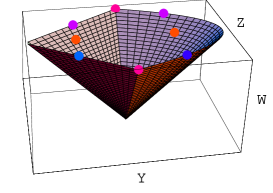
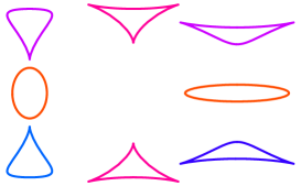
Figure 1: Each point $\{W,Y,Z\}$ in the cone on the left corresponds to a two dimensional curve that does not self intersect shown on the right. The colors of the shapes (right) matches the color of the dots (left). The two ellipses correspond to the two interior points. The six shapes with cusps correspond to the six points on the boundary of the physical cone.

The Physical cone: A physical shape does not self-intersect. Since there are points $\{W,Y,Z\}\in\mathbb{R}^{3}$ which represent curves that self-intersect, e.g. $Z=0$, $W=\pm Y$, we need to remove them. The physical shapes make a cone, for if $\{W,Y,Z\}$ does not self-intersect neither does $\lambda\{W,Y,Z\}$ with $\lambda>0$. The shapes associated with points in the interior of the cone are smooth. Points on its boundary correspond to shapes with cusp-like singularities (precursors of self-intersections). The boundary of the physical cone is given by those $\{W,Y,Z\}$ for which there exists $\zeta$ of unit modulus such that $z^{\prime}(\zeta)=0$. One finds that the physical cone around the $W$ axis is bounded by two planes and a quadratic surface and is given by , see Fig. 1,

$$W\geq Y\pm\sqrt{2}\,Z\,,\quad WY\geq 2Z^{2}-W^{2}\ .$$ (11)

Optimization and orbits in magnetic fields: Admissible strokes are closed paths $\gamma$ that lie in the physical cone. Consider the problem of minimizing the dissipation, $D(\gamma)$, of Eq. (9) subject to the constraint that the step size is

$$X(\gamma)=\oint_{\gamma}A\,dY\,.$$ (12)

This is a standard problem in variational calculus. Note that since one may set $\tau=1$ without loss, fixing the average speed is equivalent to fixing the step size $X(\gamma)$. The minimizer, $\gamma(t)$, must then either follow the boundary, or solve the Euler-Lagrange equation of the functional

$$S_{q}(\gamma)=4\pi\mu\,\int_{0}^{\tau}\big{(}\dot{W}^{2}+\dot{Y}^{2}+\dot{Z}^{2}\big{)}dt+q\int_{0}^{\tau}A\,\dot{Y}\,dt,$$ (13)

where $q$ is a Lagrange multiplier. $S_{q}$ can be interpreted as the action of a non-relativistic particle whose mass is $8\pi\mu$ and whose charge is $q$ moving in three dimensions under the action of a magnetic field with vector potential $A\hat{Y}$. $X(\gamma)$ may be interpreted as the flux of $B(W,Y,Z)=\nabla\times(A\hat{Y})$ through the closed path $\gamma$.

The parameterized stroke $\gamma(t)$ that minimizes $S_{q}$ has constant velocity $|\dot{\gamma}|=const$. (This follows from the fact that the flux $X(\gamma)$ is independent of parametrization and that the action of a free particle along a one dimensional curve is minimized at constant speed.) The dissipation is then $D(\gamma)=4\pi\mu\frac{|\gamma|^{2}}{\tau}$, where $|\gamma|$ is the length of the orbit, and the drag $\delta(\gamma)$ is simply:

$$\delta(\gamma)=\left(\frac{|\gamma|}{X(\gamma)}\right)^{2}\ .$$ (14)

Since the variational problem is for a domain with non-smooth boundaries, Fig. 1, one may worry if the minimizer fails to be smooth. This is not the case. For if $\gamma(t)$ has a corner, smoothing the corner on a scale $\varepsilon$ shortens the length $|\gamma|$ by $O(\varepsilon)$ while $|X(\gamma)|$ varies by $O(\varepsilon^{2})$. In particular, it follows that the minimizer avoids the corners of the physical cone. Moreover, whenever it hits or leaves the boundary of the physical cone, it does that tangentially, without corners.

Incompressible swimmers: Incompressible swimmers make a natural (and biologically important) class of swimmers. In two dimensions incompressibility implies constant area. The area of the swimmer whose shape is given by Eq. (3) is

$$\frac{1}{2}\,\mathop{\mathrm{missing}}{Im}\,\oint\bar{z}\,dz=\pi(W^{2}-Y^{2}-Z^{2})\,.$$ (15)

Fixing the area of the swimmer corresponds to restricting the stroke to a hyperboloid in shape space. We choose the unit of area so that the area of the swimmer is $\pi$. The intersection of the constant area hyperboloid with the cone of physical shapes is the Big-Ben shaped surface shown in Fig. 2. Physical strokes are represented by closed paths that lie inside this domain, and our aim is to find the stroke that minimizes the swimming drag $\delta(\gamma)$.

Large strokes are inefficient: The model admits strokes that extend to arbitrarily large values of $Y$ and $W$. Since, by Eqs. (7,11,12), the total flux of $B$ through the Big-Ben shaped region of Fig. 2 is infinite, the swimmer can swim arbitrarily large distances with a single stroke. However, as we presently show, large strokes are inefficient. The domain of physical incompressible shapes for a swimmer of area $\pi$ is contained in the strip $|Z|\leq 1$. Since $A=O(\frac{1}{Y})$, for $Y$ large, a long excursion, of order $\ell$, in the $Y$ direction contributes $O(\log\ell)$ to $X(\gamma)$, but $O(\ell)$ to $|\gamma|$. Therefore, as $\ell\to\infty$ the drag coefficient $\delta$ diverges like $\ell/\log\ell$.

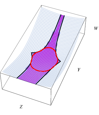
Figure 2: The Big-Ben shaped surface is the intersection of the physical cone (no self-intersection) with the hyperboloid of shapes with fixed area. The boundary of the domain of incompressible non-self-intersecting shapes is drawn black. The inscribed red curve is the optimal stroke as computed numerically.

The minimizer: Since the drag diverges for small strokes and also for large strokes (for an incompressible physical swimmer) the minimizer of $\delta$ is a finite stroke. It can be computed numerically using the following procedure: Since the minimizer is independent of the period $\tau$, one may, without loss, restrict oneself to orbits with fixed energy, say $E=1$. Pick the charge $q$ and find a smooth and closed orbit on the hyperboloid of constant area with (four) sections in the interior of the cone of physical shapes and (four) sections on its boundary. There is a unique such orbit $\gamma_{q}$ for all $q$ that are small enough. For each such orbit one computes, numerically, $X(\gamma_{q})$, and $|\gamma_{q}|$ to get $\delta(\gamma_{q})$ from Eq. (14). What remains is a minimization problem in one variable, $q$, which yields the optimal stroke. The optimal stroke in shape space is shown in Fig. 2 while snapshots of the corresponding swimming motion in real space are shown in Fig. 3. For the optimal stroke we find $\delta_{\rm{optimal}}\approx 9.12\ .$ For the sake of comparison with a squirming circle consider $\gamma$ which is a small circle of radius $r$ in the $Y-Z$ plane, centered at $Y=Z=0,W=W_{0}$. One readily finds from Eqs. (7,14) that $\delta=8(W_{0}/r)^{2}$. A squirmer that changes it shape by 10% has, $r/W_{0}=0.1$, and $\delta=800$.

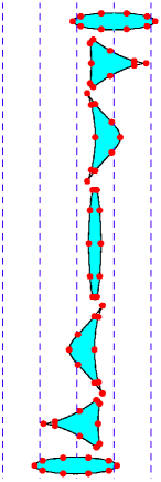
Figure 3: Snapshots of the optimal swimmer shifted vertically for visibility. The top and bottom snapshots are related by a (horizontal) translation. The shapes with cusps correspond to those parts of the stroke that lie on the boundary of the domain of simple shapes. The (red) dots are fixed reference points in the body. When the swimmer is approximately triangular, the base of the triangle functions as an anchor that pushes or pulls the opposite vertex.

Perspective: The optimal swimmer we have found is optimal within the class of Riemann maps of Eq. (3) satisfying incompressibility. Enlarging the class of Riemann maps, would allow for better swimmers. It is conceivable that there are superior swimmers that use quite different swimming styles. The importance of the model lies in that it demonstrates a scheme for a systematic search of efficient swimmers, and provides benchmark for $\delta$ for better swimmers to beat.

Acknowledgment: We thank E. Braun , G. Kosa, and D. Weihs for useful discussions, E. Yariv for pointing out ref. [10] and U. Sivan for proposing the problem. This work is supported in part by the EU grant HPRN-CT-2002-00277.

References

- [1] J. Lighthill, Mathematical Biofluiddynamics, SIAM, Philadelphia (1975); J. R. Blake, Math. Meth. Appl. Sci. 24, 1469 (2001).
- [2] E.M. Purcell, Am. J. Physics 45, 3-11 (1977); H. C. Berg, Physics Today, 24, January (2000).
- [3] A. Shapere and F. Wilczek, J. Fluid Mech., 198, 557-585 (1989).
- [4] H. C. Berg, Random walks in Biology, Princeton, (1983)
- [5] W. Ludwig, Zeit. f. Vergl. Physiolg. 13, 397-503, (1930); G. Taylor, Proc. Roy. Soc. (London) A 211 225-239, (1952); J. Lighthill, Comm. Pure. App. Math. 5, 109-118 (1952); J.R. Blake, J. Fluid. Mech. 46, 199-208 (1971); J. R. Blake, Bull. Austral Math. soc. 3 255 (1971).
- [6] S. Childress, Mechanics of swimming and flying, Cambridge (1981)
- [7] K. M. Ehlers, A.D. Samuel, H.C. Berg and R. Montgomery, PNAS 93, 8340-8343 (1996).
- [8] B.U. Felderhof and R.B. Jones, Physica A 202, 94, (1994); ibid 119 (1994). J. Koiller, R. Montgomery and K. Ehlers, J. Nonliear Sci. 6, 507-541 (1996); J, Koiller, M. Raup, M. Delgado, J. Ehlers and K.M. Montgomery, Comm. App. Math 17 3 (1998); H.A. Stone and A.D. Samuel, Phys. Rev. Lett. 77, 4102-4104 (1996); S. Trachtenberg, D. Fishlov, M. Ben-Artzi, Biophys. J. 85, 1345, (2003)
- [9] A. Shapere and F. Wilczek, J. Fluid Mech., 198, 587-599 (1989).
- [10] L.E. Becker, S.A. Koehler and H.A. Stone, J. Fluid Mech. 490, 15 (2003).
- [11] R. Feynman, Plenty of rooom at the bottom, APS annual meeting (1959), http://www.its.caltech.edu/ feynman/plenty.html
- [12] T. Fukuda et. al. , Proc. of Micro Electro Mechanical Systems, 300-305, (1995); S. Guo et. al. , Proc. of the 2002 Int’l Symposium on Micromechatronics and Human Science, 93-98 (2002); G. Kosa, http://robotics.technion.ac.il/ .
- [13] M. Frederick Hawthorne et. al., Science, 303, 1849 (2004).
- [14] http://physics.technion.ac.il/~avron/geometric.html
- [15] L.D. Landau and E.M. Lifshitz, Fluid Mechanics, Pergamon (1959)
- [16] N.I. Muskhelishvili, Some basic problems of the mathematical theory of elasticity, P. Noordhoff, (1963)