Hidden topological structure in the continuous Heisenberg spin chain

Abstract

In order to study the spin configurations of the classical one-dimensional Heisenberg model, we map the normalized unit vector, representing the spin, to a space curve. We show that the total chirality of the configuration is a conserved quantity. When the space curve forms a knot, this defines a new class of topological spin configurations for the Heisenberg model.

It is well known that the two-dimensional continuous Heisenberg model has very nice topological properties (Belavin and Polyakov 1975) BP . The order parameter is a normalized vector field ${\bf n}^{2}=1$ (therefore the order parameter manifold is $S^{2}$). If we impose homogenous boundary conditions on the vector field ${\bf n(r)}_{r\to\infty}={\bf n}_{0}$ ( constant vector field ), we can compactify the plane $R^{2}$ into $S^{2}$ and therefore the possible field configurations are classified by $\pi_{2}(S^{2})=\bf Z$. The energy in each class is bounded from below $H\geq nJ$, where $n$ is the number of times $S^{2}$ is wrapped around $S^{2}$, and $J$ is the coupling constant in the Heisenberg spin hamiltonian. Unfortunately the one dimensional Heisenberg model does not have this nice topological property. Under homogeneous boundary conditions the line $R^{1}$ may be compactified to $S^{1}$, and now $\pi_{1}(S^{2})=0$ and there are no different classes of configurations based on homotopy. In order to find out if there is a hidden topological structure in the one dimensional case one has to analyze the Heisenberg hamiltonian in more details. The vector field is normalized and therefore we will use the following representation for ${\bf n}=(\sin\theta\cos\phi,\sin\theta\sin\phi,\cos\theta)$. In $\theta$ and $\phi$ variables the hamiltonian has the form:

$$H=J\int_{-\infty}^{+\infty}(\theta_{s}^{2}+\sin\theta^{2}\phi_{s}^{2})ds$$

where the subscript $s$ stands for $\frac{d}{ds}$ and $s$ denotes the coordinate along $R^{1}$. This hamiltonian is not symmetric under homotety transformation $s\to\lambda s$ and therefore the spin configurations are not metastable like in the $2D$ case. The equations of motion for this spin hamiltonian have been established (Tjon and Wright 1977)) TW in taking $\phi$ and $\cos\theta$ to be the conjugated generalized coordinate and momentum so that the Poisson bracket gives $[\phi(x),\cos\theta(y)]=\delta(x-y)$. The generator of translations (momentum) is given by the following expression (Tjon and Wright 1977) TW :

$$P=\int_{-\infty}^{+\infty}(1-\cos\theta)\phi_{s}ds$$

where the third component of the normalized generator of rotations (magnetization) is given by (Tjon and Wright 1977)TW :

$$M=\int_{-\infty}^{+\infty}(\cos\theta-1)ds$$

The quantities $P$ and $M$ are constants of the motion. For our analysis of the possible spin configurations it is useful to map the unit vector $\bf n$ to the unit tangent of a space curve (Balakrishnan et al. 1990) BBD . Now different space curves will represent different spin configurations. We will impose homogeneous boundary conditions, which will assure that the energy is finite and the curves representing the different spin configurations will tend to the straight line as $s\to\pm\infty$ Now we will concentrate on the geometrical and topological quantities characterizing a space curve. Of special interest for us will be the writhe of a curve (which characterizes the chirality of the curve). It is defined as follows:

$$Wr=\frac{1}{4\pi}\int_{-\infty}^{+\infty}ds\int_{-\infty}^{+\infty}ds^{\prime}\frac{(\bf r-\bf r^{\prime}).(\bf n-\bf n^{\prime})}{|\bf r-\bf r^{\prime}|}$$

The tip of the radius vector $\bf r$ draws the curve, while $\bf n$ is the unit tangent. A theorem by Fuller (Fuller 1978)Ful allows to express $Wr$ as an integral of a local quantity. We will express $Wr$ with respect of a reference curve $C_{0}$( Fain and Rudnick 1997)DNA :

$$Wr=Wr_{0}+\frac{1}{2\pi}\int_{-\infty}^{+\infty}\frac{{\bf n}_{0}\times{\bf n}.\frac{d}{ds}({\bf n}_{0}+{\bf n})}{(1+{\bf n}_{0}.{\bf n})}ds$$

where $Wr_{0}$ is the writhe of the reference curve. The simplest choice is the straight line $C_{0}=(0,0,s)$, then ${\bf n}_{0}=(0,0,1)$ and $Wr_{0}=0$( Fain and Rudnick 1997)DNA . A simple calculation gives the following expression for the writhe:

$$Wr=\frac{1}{2\pi}\int_{-\infty}^{+\infty}(1-\cos\theta)\phi_{s}ds$$

Our first observation is that the writhe $Wr$ for the spin configurations (quantity that characterizes the chirality of the spin configuration) coincides with the total momentum $P$. The total momentum $P$ is a conserved quantity - it follows that $Wr$ is a conserved quantity too. This will lead us to a new class of possible excitations for the continuous classical spin Heisenberg model. We will note first that the writhe $Wr$ suffers discontinuity when one region of the curve crosses another and the jump is always +2(Frank-Kamenetskii and Vologodskii)Uspehi . This means that all configurations that belong to the configuration of the ground state ($\theta=0$) are separated from all other classes of configurations by a jump of the writhe $Wr$. Let us consider one such configuration: the space curve representing the spin configuration forms a knot with a loop which follows the semi-circle at infinity and then comes back from $s=\pm\infty$ as a straight line and goes into the actual knot. One can imagine also a knot which is cut at $s=s_{0}$ and then both ends are pulled to $+\infty$ and $-\infty$ and are put together over the infinite semi-circle (see Fig.1). The writhe is zero for both straight segments when $s\to\pm\infty$ and for the infinite semi-circle. This geometrical construction does not change the writhe of the actual knot. Such a knot belongs to a whole class of configurations which deform smoothly from one to another and who are separated from the ground state class by a jump in the writhe $Wr$. Belonging to the knot configuration will have consequences for the energy of the spin configuration too. Let us consider the following Cauchy-Schwarz inequality:

$$\int_{-\infty}^{+\infty}\sin^{2}\frac{\theta}{2}ds\int_{-\infty}^{+\infty}\phi_{s}^{2}\sin^{2}\frac{\theta}{2}\geq$$

$$\geq\left(\int_{-\infty}^{+\infty}\phi_{s}\sin^{2}\frac{\theta}{2}ds\right)^{2}=\frac{P^{2}}{4}$$

The energy satisfies the obvious inequality:

$$J\int_{-\infty}^{+\infty}(\theta_{s}^{2}+\sin^{2}\theta\phi_{s}^{2})ds=J\int_{-\infty}^{+\infty}(\theta_{s}^{2}+4\sin^{2}\frac{\theta}{2}\phi_{s}^{2})ds\geq$$

$$\geq J\int_{-\infty}^{+\infty}4\sin^{2}\frac{\theta}{2}\phi_{s}^{2}ds$$

Combining inequalities (7) and (8) leads to the following inequality for the energy:

$$H\geq J\frac{P^{2}}{M}$$

Let us note here that $M=0$ only for the ground state $\theta=0$ and that $P\neq 0$ for curves in the knot configuration. Thus the energy is limited from below for such a configuration.

We have shown that there are topological configurations for the Heisenberg spin model even in the one-dimensional case. One should investigate the different knot configurations in order to elaborate a classification of such configurations according to the type of knot they represent.

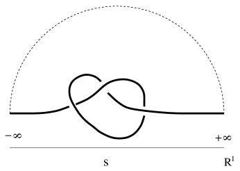
Figure 1: Spin configuration

References

- (1) A A Belavin and A M Polyakov, (1975), JETP Lett. 22, 245.
- (2) J. Tjon and Jon Wright, (1977), Phys. Rev. B 15, 3470.
- (3) Radha Balakrishnan, A.R. Bishop, and R. Dandoloff, (1990), Phys.Rev.Lett., 64, 2107.
- (4) F.B. Fuller, (1978), Proc.Natl.Acad.Sci.USA 75 , 3357.
- (5) B.Fain and J. Rudnick, (1997), Phys.Rev. E, 55, 7364.
- (6) M.D. Frank-Kamenetskii and A.V. Vologodskii, (1981), Sov.Phys.Usp. 24(8), 679.