Whitham hierarchy in growth problems

We discuss the recently established equivalence between the Laplacian growth in the limit of zero surface tension and the universal Whitham hierarchy known in soliton theory. This equivalence allows one to distinguish a class of exact solutions to the Laplacian growth problem in the multiply-connected case. These solutions corerespond to finite-dimensional reductions of the Whitham hierarchy representable as equations of hydrodynamic type which are solvable by means of the generalized hodograph method.

1 Introduction

Dynamics of a moving front (an interface) between two distinct phases driven by a harmonic scalar field often appears in different physical and mathematical contexts and has a number of important practical applications. Processes of this type are unified by the name of Laplacian growth. Their key common feature is a harmonic field which serves as a potential for the growth velocity field.

The most extensively studied is the case of two-dimensional spatial geometry. To be definite, we shall speak about an interface between two immiscable and incompressible fluids with very different viscosities on the plane. In practice the 2D geometry is realized in a narrow gap between two parallel glass plates (the Hele-Shaw cell). In this version, the problem is also known as the Saffman-Taylor problem. For a review, see [1].

To be more precise, consider a compact plane domain occupied by a fluid with a negligible viscosity (water). We call it water droplet. Let its exterior be occupied by a viscous fluid (oil). The oil/water interface is assumed to be a smooth closed contour. Oil is sucked out with a constant rate through a sink (a pump) placed at some fixed point (which may be at infinity) while water is injected into the water droplet. More generally, one may consider several oil pumps and several disconnected water droplets. In this general setting the problem was discussed in [2]-[6].

In the oil domain, the local velocity $\vec{V}=(V_{x},V_{y})$ of the fluid is proportional to the gradient of pressure $p=p(x,y)$ (Darcy’s law):

$$\vec{V}=-\kappa\nabla p$$

where $\kappa$ is called the filtration coefficient. It is inversely proportional to viscosity of the fluid. For future convenience, we choose units in such a way that $\kappa$ for oil be equal to $\frac{1}{4}$. In particular, the Darcy law holds on the outer side of the interface thus governing its dynamics: $V_{n}=-\frac{1}{4}\partial_{n}p$. Here $V_{n}$ is the growth velocity, which is by definition normal to the interface, and $\partial_{n}$ is the normal derivative. Since the fluids are incompressible ($\nabla\vec{V}=0$) the Darcy law implies that pressure $p$ is a harmonic function in the exterior (oil) domain except at the point where the oil pump is placed. There is a logarithmic singularity at this point.

So, the pressure field is a solution of the time-dependent boundary value problem for the Laplace operator $\Delta=\partial_{x}^{2}+\partial_{y}^{2}$ with a prescribed logarithmic singularity and with certain condition on the boundary of the growing domain. This condition is fixed by the following reasoning. If viscosity of water is small enough, pressure is uniform inside water droplets ($p=\mbox{const}$). Hereafter, we assume that pressure does not jump across the boundary, so the function $p(x,y)$ is constant along it. This means that the surface tension is set to be zero. To summarize, the mathematical formulation of the Laplacian growth, in the limit of zero surface tension, is:

$$\begin{array}[]{l}V_{n}=-\frac{1}{4}\partial_{n}p\,,\\ \Delta p=0\quad\mbox{in oil with $dp=0$ along the boundary,}\\ p(x,y)=\log\rho^{2}+...\quad\mbox{as $\rho\to 0$}\end{array}$$ (1)

Here $\rho$ is the distance between the sink and the point $x,y$. If the sink is at infinity, what is often assumed in the outer growth problem, the last condition is replaced by the asymptotics $p=-\log(x^{2}+y^{2})+\ldots$ very far away from the droplet. If the oil domain is multiply-connected (i.e., there are more than one water droplet), this formulation should be supplemented by some additional physical conditions for pressure in the water droplets, which we do not discuss here. The problem consists in finding the time evolution of the interface between the fluids.

The simply-connected case (one water droplet) allows for an effective application of the conformal mapping technique (see, e.g., [1, 5]). Passing to the complex coordinates $z=x+iy$, $\bar{z}=x-iy$, one may describe the growth process in terms of a time dependent conformal map $z=f(w,T)$ from a fixed domain of a simple form, say the exterior of the unit disk, onto the evolving oil domain. The interface itself is the image of the unit circle $w=e^{i\phi}$, $0\leq\phi\leq 2\pi$. The dynamics (1) is then translated to a nonlinear partial differential equation for the function $f(w,T)$, referred to as the Laplacian growth equation. If the oil sink is at infinity, it reads

$$2{\rm Im}\,\left(\frac{\partial f(e^{i\phi},T)}{\partial\phi}\,\overline{\frac{\partial f(e^{i\phi},T)}{\partial T}}\right)=1$$ (2)

It first appeared in 1945 in the works [7] on the mathematical theory of oil production.

Later, some exact finite dimensional reductions of the Laplacian growth equation were found. Asuming that the derivative of the conformal map $f$ is a rational function, it reduces, upon a direct substitution, to a finite dynamical system for parameters of this function (say, for its poles, zeros or residues). See [8], [9] for different versions of such dynamical systems. Moreover, it turnes out that these systems can be actually integrated in the sense that all time derivatives are removable. As a result, the poles are represented as implicit functions of time.

Existence of finite-dimensional reductions was a serious motivation for searching an underlying integrable structure of the model. In case of one water droplet, such a structure was identified in [10] to be the 2D Toda hierarchy in the limit of zero dispersion. The Laplacian growth equation is the string equation of the Toda hierarchy. The conformal map plays the role of the Lax function.

The vector field $\partial/\partial T$ in the space of domains defines a particular flow of the Toda hierarchy. Other flows are “frozen” until oil is sucked by a single pump only. To “unfroze” them, one should allow oil pumps to work at any point in the plane. In general there are as many flows as types and locations of oil pumps. It is convenient to associate to each pump its own time variable which is the total amount of oil sucked by the pump. It is known [6] that the result of the Laplacian growth evolution, in the case of several pumps, depends only on the total amount of oil sucked by each of them and does not depend on the order in which they operate. In the context of integrable systems, this fact reflects commutativity of flows of the Toda hierarchy.

Recently, this approach was extended [11] to the Laplacian growth of several water droplets. In this case the dynamics turns out to be equivalent to the universal Whitham hierarchy on the moduli space of genus $g$ Riemann surfaces, where $g$ is the number of water droplets minus 1. In full generality, this hierarchy was introduced by Krichever [12, 13] in the context of slow modulations of exact periodic solutions to soliton equations. The dispersionless Toda hierarchy is its simplest particular case at $g=0$. The universal Whitham hierarchy is known to have a lot of meaningful finite-dimensional reductions for any $g$. They are systems of differential equations of hydrodynamic type which can be implicitly solved by the generalized hodograph method [14]. Applying these results to the Laplacian growth problem, we obtain a large family of solutions in the multiply-connected case. The infinite dimensional contour dynamics for them is reduced to finite systems of differential equations which can be integrated.

The aim of the present paper is to study this class of finite-dimensional reductions and to clarify their algebro-geometric meaning.

2 Laplacian flows and the universal Whitham hierarchy

In this section we explain the precise meaning of the statement that the Laplacian growth is described by the Whitham equations.

We use the following notation (Fig. 1). Let ${\sf D_{\rm oil}}$ be the region of the plane occupied by oil (a non-compact domain containing infinity), and ${\sf D}$ be the region occupied by water. We assume that there are $g+1$ water droplets, which are compact domains bounded by smooth non-intersecting closed contours $\gamma_{\alpha}$, $\alpha=0,1,\ldots,g$. Let ${\sf D}_{\alpha}$ be the $\alpha$-th water droplet, so that ${\sf D}$ is their union. By $\gamma$ we denote the union of the $\gamma_{\alpha}$’s: $\gamma=\cup_{\alpha=0}^{g}\gamma_{\alpha}$. Our assumptions imply that no contour $\gamma_{\alpha}$ lies inside another.

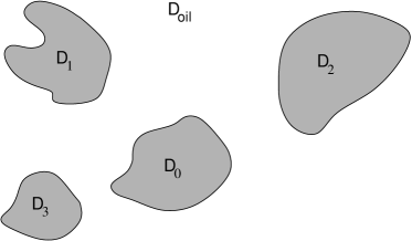
Figure 1: Water droplets ${\sf D}_{\alpha}$ ($g=3$).

2.1 Commutativity of Laplacian flows

Any growth process defines a flow in the space of contours, or, in the infinitesimal version, a vector field. Integral curves of this vector field are just one-parametric families of contours $\gamma(T)$ obtained from any initial contour $\gamma(0)$ by the evolution in the time $T$.

Flows corresponding to the Laplacian growth (Laplacian flows) are determined by location of oil pumps. Namely, given an oil sink at a point $a\in{\sf D_{\rm oil}}$, the solution of the boundary value problem

$$\Delta p(z)=4\pi\delta^{(2)}(z-a)\,,\quad\quad dp=0\;\mbox{on $\gamma$}$$ (3)

in ${\sf D_{\rm oil}}$ (here $\delta^{(2)}(z-a)$ is the two-dimensional delta-function supported at the point $a$), with some additional conditions on the boundaries of ${\sf D}_{\alpha}$’s in case of more than one water droplet (see [11] for details), uniquely defines an infinitesimal deformation of $\gamma$ by setting the vector of normal velocity to be $-\frac{1}{4}\partial_{n}p$. Such a deformation is a tangent vector to the space of contours. For brevity, in this paper we do not discuss other types of Laplacian flows considered in [11].

Given a Laplacian flow, a natural parameter along the trajectories in the space of contours is the amount of oil, $T$, sucked by the pump which defines the flow. Since the both fluids are assumed to be incompressible, $T$ is simply the change of the total area of the water droplets. (If the pumping rate is constant, $T$ can be also identified with time.) Let $\partial_{T}$ be the corresponding vector field. It is defined in an invariant way, i.e., it does not depend on the choice of local coordinates in the space of contours.

As is common, we identify vector fields with derivatives along them. The derivative of any functional $F$ on the space of contours along the vector field (the Lie derivative) is defined as follows:

$$\partial_{T}F=\lim_{\epsilon\to 0}\frac{F(\gamma(T+\epsilon))-F(\gamma(T))}{\epsilon}$$

If there are several sinks (at the points $a$, $b$, etc), we write $\partial_{T^{(a)}}$, $\partial_{T^{(b)}}$, etc for the corresponding vector fields.

The notation is justified by the following theorem [6].

Theorem 1. The vector fields $\partial_{T^{(a)}}$, $\partial_{T^{(b)}}$ commute for all $a,b\in{\sf D_{\rm oil}}$.

It is an infinitesimal formulation of the fact that the result of the Laplacian growth evolution (i.e., the shape of ${\sf D_{\rm oil}}$) depends only on the amounts of oil $T^{(a)}$, $T^{(b)}$ sucked from the points $a$, $b$ and does not depend on other details of the process (assuming that no topological change or singularity occurs). In its turn, this fact follows from the reduction of the Laplacian growth to the inverse potential problem in two dimensions and from local uniqueness of solutions to the latter. For more details see [6].

This result suggests to treat $\partial_{T^{(a)}}$ as a partial derivative in a space with coordinates $T^{(a)}$. To construct a simple example of such a space, fix $N$ points $a_{j}$ and consider the variety of contours which can be obtained from some initial configuration as a result of all Laplacian growth processes with oil pumps at the points $a_{j}$. The resulting shape of the droplets is uniquely determined (if no singularity occurs) by amounts of oil sucked out of each point $a_{j}$, i.e., by the quantities $T^{(a_{j})}$. This configuration space is $N$-dimensional and $T^{(a_{j})}$ are local coordinates in it.

2.2 The Schottky double

Our next task is to carry the Laplacian flows over to compact Riemann surfaces with a real structure. To do that we need the Schottky double construction [15] which we recall here.

With the domain ${\sf D_{\rm oil}}$ (as well as with any plane domain with a boundary) one canonically associates its Schottky double

$${\mit\Sigma}={\sf D_{\rm oil}}\cup\gamma\cup{\sf D}_{\rm oil}^{*}$$

where ${\sf D}_{\rm oil}^{*}$ is another copy of ${\sf D_{\rm oil}}$ (its “opposite side”) attached to it along the boundary $\gamma$. In what follows, we shall call ${\sf D_{\rm oil}}$ and ${\sf D}_{\rm oil}^{*}$ the front side and the back side of the double, respectively. Formally speaking, a point $P\in{\mit\Sigma}$ is a pair $P=(z,\sigma)$, where $z\in{\sf D_{\rm oil}}$ and $\sigma=\pm$ indicates front or back side. If $z\in\gamma$, the pairs $(z,\pm)$ represent the same point. There is a natural projection ${\mit\Sigma}\rightarrow{\sf D_{\rm oil}}$ which sends a point $P=(z,\sigma)\in{\mit\Sigma}$ to the point $z\in{\sf D_{\rm oil}}$. In the sequel, we sometimes write simply $z$ for $(z,+)$ and $z^{*}$ for $(z,-)$.

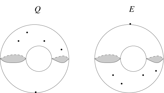
Figure 2: Poles of the functions $Q$ and $E$ on the Schottky double ($g=1$). The upper and lower halves of the torus give a schematic view of the front and back sides of the double, respectively.

By adding a point at infinity for each copy of ${\sf D_{\rm oil}}$, ${\mit\Sigma}$ becomes a compact surface naturally endowed with a complex structure. The complex structure on the front side is the same as in ${\sf D_{\rm oil}}$ while the back side has the opposite complex structure. In other words, the holomorphic coordinate is $z$ on ${\sf D_{\rm oil}}$ and $\bar{z}$ on ${\sf D}_{\rm oil}^{*}$. Whence ${\mit\Sigma}$ is a compact Riemann surface with the antiholomorphic involution $P\mapsto P^{*}$ which sends $(z,\sigma)$ to $(z,-\sigma)$. The two sides of the double are in a sense mirror images of each other, so we shall call points connected by the involution mirror-symmetric points. Boundaries of the droplets are fixed points of the involution. A schematic view of the Schottky double see in Fig. 2 below.

If the contours $\gamma_{\alpha}$ are smooth, the double is, by construction, a smooth Riemann surface of genus $g$. Indeed, each point of ${\mit\Sigma}$, including points of the boundary of ${\sf D_{\rm oil}}$, has a disk-like neighborhood.

Note that the set of fixed points of the involution consists of exactly $g+1$ closed contours, which is the maximal possible number for surfaces of genus $g$. Riemann surfaces with antiholomorphic involution having this property are called real.

In what follows it is implied that a canonical basis of ${\sf a}$ and ${\sf b}$-cycles on the double is fixed. This can be done in many ways. For example, one may take ${\sf a}_{\alpha}$-cycles to be boundaries of the droplets ${\sf D}_{\alpha}$ for $\alpha=1,\ldots,g$ and take ${\sf b}_{\alpha}$-cycles to be some paths connecting the boundary of the $0$-th droplet with the $\alpha$-th one on the front side and going back through the opposite side of the double. Each choice of the basis of cycles corresponds to certain physical conditions in the water droplets which are discussed in detail in [11]. For our purpose here it is enough to imply that one or another basis is fixed.

Any pair of meromorphic functions $\varphi,\tilde{\varphi}$ (which are functions on ${\sf D_{\rm oil}}$ and on the complex congugate domain respectively) such that $\varphi(z)=\tilde{\varphi}(\bar{z})$ on the boundary defines a meromorphic function on the double. Namely, this function takes the value $\varphi(z)$ at the point $z$ on the front side and the value $\tilde{\varphi}(\bar{z})$ at the mirror-symmetric point $z^{*}$ on the back side. Similarly, a meromorphic differential on the double is represented by a pair of meromorphic differentials $\varphi(z)dz$ and $\tilde{\varphi}(\bar{z})d\bar{z}$ such that $\varphi(z)dz=\tilde{\varphi}(\bar{z})d\bar{z}$ along the boundary contours.

If a meromorphic differential $d\omega(z)$ on ${\sf D_{\rm oil}}$ is purely imaginary along the boundary, the analytic continuation to the opposite side of the double is especially simple. Indeed, in accord with the Schwarz reflection principle, its meromorphic extension to the back side is $-\overline{d\omega(z)}$, so for each pole of such a globally defined differential there is a mirror pole on the opposite side. In this case we shall say that $d\omega$ is a symmetric differential on ${\mit\Sigma}$.

2.3 Abelian differentials on the double

To each pump we assign an Abelian differential on ${\mit\Sigma}$. On the front side it is the differential $\partial_{z}pdz$, where $p$ is the pressure field generated by the pump in the viscous fluid. Since $dp=\partial_{z}pdz+\partial_{\bar{z}}pd\bar{z}=0$ on the boundary, $\partial_{z}pdz$ is purely imaginary along the boundary. So, its analytic continuation to the back side of the double is $-\partial_{\bar{z}}pd\bar{z}$. Conversely, given a symmetric Abelian differential on ${\mit\Sigma}$, we place pumps at its poles on the front side. Strengths of the pumps are determined by the residues.

Note also that any symmetric Abelian differential $d\Omega$ on ${\mit\Sigma}$ defines a tangent vector to the space of contours via setting the normal velocity at any point of the contour to be

$$V_{n}=-\frac{1}{2}\partial_{n}\,{\rm Re}\int^{z}d\Omega$$

If poles of $d\Omega$ are fixed in the $z$-plane, this defines a vector field corresponding to a Laplacian flow.

For example, if oil is sucked (with a unit rate) from a point $a\in{\sf D_{\rm oil}}$, then

$$p(z)=2G(a,z)$$

where $G$ is the Green function of the Dirichlet problem in ${\sf D_{\rm oil}}$. The Green function is defined as a solution of the Laplace equation in ${\sf D_{\rm oil}}$ with the logarithmic singularity of the form $G(a,z)\to\log|z-a|$ as $z\to a$ and such that $dG=0$ on the boundaries. Therefore, the differential $dW^{(a)}(z)=\partial_{z}pdz$ has a simple pole at $z=a$ with the residue 1 and no other singularities in ${\sf D_{\rm oil}}$. The analytic continuation of this differential to the back side is $-\overline{dW^{(a)}(z)}$ which gives a simple pole at the mirror point $a^{*}$ with the residue $-1$. The differential constructed is a symmetric Abelian differential of the third kind (a dipole differential):

$$dW^{(a)}=\left\{\begin{array}[]{cc}2\partial_{z}G(a,z)dz&\mbox{on the front side}\\ &\\ -2\partial_{\bar{z}}G(a,z)d\bar{z}&\mbox{on the back side}\end{array}\right.$$ (4)

Remark. For $g\geq 1$ these conditions do not yet define the differential uniquely. To fix it, a normalization is needed. We normalize the differential $dW^{(a)}$ by the condition that it has zero ${\sf a}$-periods. Depending on the choice of cycles, this means certain physical conditions: for instance, fixed injecting rates or fixed pressures in the water droplets. See [11] for details.

2.4 The Whitham hierarchy

The Whitham hierarchy structure reveals itself in evolution of the Abelian differentials under Laplacian flows ${\mit\Sigma}\to{\mit\Sigma}(T)$.

The holomorphic coordinate $z$ on the front side of ${\mit\Sigma}$ is independent of time by construction. It defines a connection in the space of real Riemann surfaces of genus $g$. Correspondingly, the Abelian differentials become time dependent: $dW=dW(z,T)$. At any fixed $z$, $dW(z)$ is a functional on the space of contours, so one can take derivatives along Laplacian vector fields.

In [11], it was shown that the Laplacian growth of ${\sf D_{\rm oil}}$, with zero surface tension, is equivalent to the system of Whitham equations for symmetric Abelian differentials of the third kind $dW^{(a)}$ on the Schottky double of ${\sf D_{\rm oil}}$. The main result is the following theorem [11]:

Theorem 2. For any pair of pumps (at the points $a,b\in{\sf D_{\rm oil}}$), the following relations hold:

$$\partial_{T^{(a)}}\,dW^{(b)}=\partial_{T^{(b)}}\,dW^{(a)}$$ (5)

This statement follows from (4) and the Hadamard variational formula [16] for the Green function $G(z,a)$. The Hadamard formula implies that $\partial_{T^{(a)}}G(b,c)$ is symmetric under permutations of the points $a,b,c$.

The theorem allows one to identify Laplacian flows with Whitham flows on the (extended) moduli space of real Riemann surfaces. Equations (5) constitute the universal Whitham hierarchy [13]. In the soliton theory, they are obtained by averaging solutions of soliton equations over fast oscillations [17].

Since the Laplacian vector fields commute, one may look for a general solution to equations (5) in the form

$$dW^{(a)}=-\partial_{T^{(a)}}d\Omega$$ (6)

where $d\Omega$ is called the generating differential.

Remark. In general, singularities of the generating differential may be of a very complicated nature. Equations (6) mean, however, that all of them do not move under the Laplacian flows. In other words, they are integrals of motion. The only parameter that changes in the course of the Laplacian growth with a sink at the point $a$ is the residue of $d\Omega$ at the pole at $a$. This means, in particular, that the Laplacian flows with point-like pumps can only add simple poles to singularities of $d\Omega$.

In the next section we consider an important special case when all singularities of the generating differential are poles, i.e., $d\Omega$ is meromorphic on ${\mit\Sigma}$.

3 Algebraic domains

Families of special solutions to the Whitham equations with a meromorphic generating differential were constructed in [12]. In [11], it has been shown that they describe Laplacian growth of algebraic domains. It is clear that an algebraic domain remains algebraic under Laplacian flows with point-like pumps. This fact allows one to reduce the infinite dimensional configuration space of contours to a finite dimensional one.

3.1 The Schwarz function

For a more explicit characterization of the class of algebraic domains that we are going to deal with, consider the analytic continuation of the function $z$ defined in ${\sf D_{\rm oil}}$ to the back side of the Shottky double.

Definition. The domain ${\sf D_{\rm oil}}$ is said to be algebraic if the function $z$ is extendable to a meromorphic function on the Schottky double of ${\sf D_{\rm oil}}$.

To clarify the meaning of this definiton, we recall the notion of the Schwarz function [18]. Given a bounded plane domain, the Schwarz function is the analytic continuation of the function $\bar{z}$ away from the boundary. Note that for such an analytic continuation to exist, the boundary needs to be analytic, not only smooth. By definition, the Schwarz function, $S(z)$, is a function analytic in some neighborhood of the boundary contour (contours) such that

$$S(z)=\bar{z}\;\;\;\;\mbox{on the contour}$$

If it exists, the Schwarz function must obey the “unitarity condition”

$$S(\overline{S(z)})=\bar{z}$$

which means that the function $\overline{S(\bar{z})}$ is inverse to $S(z)$. In general, the analytic continuations from different components of the boundary of a multiply-connected domain may lead to different functions. Algebraic domains correspond to a rather special situation when they lead to a common function which is well-defined everywhere in ${\sf D_{\rm oil}}$.

If the Schwarz function exists, the analytic continuation of the function $z$ to the back side is just $\overline{S(z)}$. Therefore, a plane domain is algebraic if and only if the Schwarz function is extendable to a meromorphic function in it.

Let $P\in{\mit\Sigma}$ be a point on the Schottky double of an algebraic domain. Consider the function $Q(P)$ on ${\mit\Sigma}$ defined as follows:

$$Q(P)=\left\{\begin{array}[]{cc}S(z)&\;\;\mbox{if $P$ is on the front side}\\ &\\ \bar{z}&\;\;\mbox{if $P$ is on the back side}\end{array}\right.$$

Here $z=z(P)$ is the $z$-coordinate of the point $P=(z,\sigma)$ on ${\mit\Sigma}$. By definition of the Schwarz function, $Q(P)$ extends continuously across the contour $\gamma$ and so it is a well-defined meromorphic function on ${\mit\Sigma}$. Along with the $Q(P)$, we introduce a “mirror-symmetric” function

$$E(P)=\left\{\begin{array}[]{cc}z&\;\;\mbox{if $P$ is on the front side}\\ &\\ \overline{S(z)}&\;\;\mbox{if $P$ is on the back side}\end{array}\right.$$

which is meromorphic on ${\mit\Sigma}$ as well. It provides the above mentioned meromorphic extension of the function $z$ to the whole double. Note that the functions $Q$, $E$ are connected by the relation

$$S(E(P))=Q(P)$$ (7)

and transform one into another (with complex conjugation) under the antiholomorphic involution:

$$Q(P^{*})=\overline{E(P)}$$ (8)

Suppose that the Schwarz function in ${\sf D_{\rm oil}}$ has poles at some points $p_{j}\in{\sf D_{\rm oil}}$ with multiplicities $n_{j}$. Hereafter, the points $p_{j}$ are assumed to be in general position. Set $N=\sum_{j}n_{j}$. Then the number of droplets can not exceed $N+1$, or, what is the same, genus of the Schottky double is less or equal to $N$:

$$g\leq N=\sum_{j}n_{j}$$

This rough estimate follows from the fact that any nontrivial function on a Riemann surface of genus $g$ has at least $g+1$ poles counted with multiplicities (if everything is in general position). Applying this statement to the function $Q$, we get the estimate.

To summarize, on the Schottky double of an algebraic domain there exist two meromorphic functions connected by the involution as in (8). The notation $Q$, $E$ is chosen to emphasize the similarity with the approach developed in [13].

Remark. The class of algebraic domains introduced here and in [6] coincides with the class of “quadrature domains” from [19]. The class of domains corresponding to “algebraic orbits” of the Whitham equations [13] is broader. It includes domains for which the generating differential is meromorphic on ${\mit\Sigma}$ with “jumps” across certain cycles.

3.2 A complex curve associated with an algebraic domain

For algebraic domains, the Schwarz function is an algebraic function, i.e., it satisfies a polynomial equation $R(S(z),z)=0$. The easiest way to see this is to consider the analytical continuations of the functions $z$, $S(z)$ to the whole double, i.e., the functions $E,Q$.

If $S(z)$ has $N$ poles in ${\sf D_{\rm oil}}$ (counting multiplicities), then the function $Q$ has $N+1$ poles on ${\mit\Sigma}$ ($N$ poles on the front side and a simple pole at infinity on the back side). Similarly, the function $E$ also has $N+1$ poles. Therefore, we have two meromorphic functions with $N+1$ poles on a smooth Riemann surface. A simple theorem of algebraic geometry states that these functions are connected by a polynomial equation of degree $N+1$ in each variable:

$$R(Q,E)=\sum_{n,m=0}^{N+1}A_{nm}Q^{n}E^{m}=0$$ (9)

Symmetry under the involution implies that the matrix of coefficients is Hermitian: $A_{nm}=\overline{A_{mn}}$. Restricting the relation between $Q$ and $E$ to the front side of the double, we get the polynomial equation

$$R(S(z),z)=0$$

The unitarity condition for the Schwarz function is equivalent to the hermiticity of coefficients of this polynomial.

The equation $R(\tilde{z},z)=0$ defines a complex algebraic curve ${\mit\Gamma}$ which may serve as another realization of the Riemann surface ${\mit\Sigma}$. The boundary contour is recovered as the set of real solutions $x,y$ to the equation $R(x-iy,\,x+iy)=0$. It is the real section of the curve ${\mit\Gamma}$.

Remark. We see that the boundary of any algebraic domain is always described by a polynomial equation. The converse is not true. An arbitrary polynomial equation with hermitian coefficients in general does not define an algebraic domain.

Despite of the fact that ${\mit\Sigma}$ is a smooth surface, the curve ${\mit\Gamma}$ is not smooth for $N>0$. It contains singular points (double points in case of general position). This is seen from comparing genus of the double with the upper bound of genus of the curve ${\mit\Gamma}$. For a generic smooth curve of the form (9) genus equals $N^{2}$, so the fact that the genus does not actually exceed $N$ just gives evidence for the presence of singular points on the curve ${\mit\Gamma}$.

How do the singular points emerge? Consider the map $P\mapsto(Q(P),E(P))$ from ${\mit\Sigma}$ to ${\mit\Gamma}$ which takes a point $P$ to the pair of complex numbers $(Q(P),E(P))$ connected by the polynomial equation. If two different points of ${\mit\Sigma}$ are mapped to one point of ${\mit\Gamma}$ (i.e. values of the both functions $Q,E$ are the same at these points), then this point is clearly a singular point of the curve, namely, a self-crossing (or double) point. This situation is illustrated in Fig. 3. In short, we say that the map from the Schottky double to the curve glues some points together. This means that ${\mit\Sigma}$ in general can not be realized as a smooth algebraic curve in ${\bf C}^{2}$.

Let us give a more precise characterization of the points that can be glued together. Two distinct points $P_{1},P_{2}\in{\mit\Sigma}$ are glued together if $Q(P_{1})=Q(P_{2})$ and $E(P_{1})=E(P_{2})$. As is readily seen, this is possible only if $P_{1}$ and $P_{2}$ are on different sides of the double. Let $P_{1}=(z_{1},+)$, $P_{2}=(z_{2},-)$ with $z_{1,2}\in{\sf D_{\rm oil}}$. Then these points are glued together if $S(z_{1})=\bar{z}_{2}$ and $S(z_{2})=\bar{z}_{1}$. It might seem that the second equality follows from the first one by virtue of the unitarity condition. However, the unitarity condition holds for the whole algebraic function $S(z)$ while $S(z)$ in the both equalities above means one and the same branch of the Schwarz function obtained as the analytic continuation of $\bar{z}$ to ${\sf D_{\rm oil}}$. So, we have two independent conditions to determine the points $z_{1,2}$. To put it differently, $z_{1}$ (or $z_{2}$) is a point in ${\sf D_{\rm oil}}$ where two (or more) branches of the Schwarz function take same value.

Nevertheless, the (smooth) Schottky double always has a realization as a smooth complex curve $\tilde{\mit\Gamma}$ in a higher dimensional space. This curve can be obtained from ${\mit\Gamma}$ as a result of the desingularization process. In the case of a self-crossing point this simply amounts to incorporating a third meromorphic function on ${\mit\Sigma}$, say $K(P)$, such that it takes different values at the points to be glued together by the map $P\mapsto(Q(P),E(P))$ (see Fig. 3). The curve is then defined by a system of polynomial equations $R_{1}(Q,K)=0$, $R_{2}(K,E)=0$ in ${\bf C}^{3}$. If this curve is still singular, the process should be repeated until one arrives at a smooth curve $\tilde{\mit\Gamma}$.

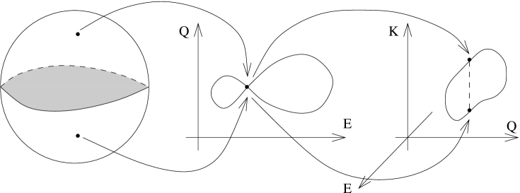
Figure 3: From a smooth Schottky double to a singular curve ${\mit\Gamma}$ and then to the smooth curve $\tilde{\mit\Gamma}$.

The so obtained smooth curve $\tilde{\mit\Gamma}$ is isomorphic to the Riemann surface of the Schwarz function. The latter can be also realized as a branched covering of the $z$-plave. In this realization, the antiholomorphic involution is the Schwarz reflection

$$z\mapsto\overline{S(z)}$$

which sends a point $z$ to its “mirror” with respect to the boundary contour.

3.3 The generating differential

The explicit form of the generating differential for algebraic domains is:

$$d\Omega=QdE=\left\{\begin{array}[]{l}S(z)dz\quad\mbox{on the front side}\\ \\ \bar{z}d\overline{S(z)}\quad\mbox{on the back side}\end{array}\right.$$

To prove this, one should check equations (6) for all vector fields $\partial_{T^{(a)}}$. These equations immediately follow from the behaviour of singularities of the Schwarz function under Laplacian flows.

Proposition. The location of poles of the Schwarz function of any algebraic domain remains unchanged under Laplacian flows with point-like pumps. The residues remain unchanged as well, except for the residue at the pole where the pump is placed:

$$\partial_{T^{(b)}}\,{\rm res}\,_{z=a}(S(z)dz)=\left\{\begin{array}[]{c}0\;\;\;\;\;\mbox{if}\quad b\neq a\\ -1\;\;\;\mbox{if}\quad b=a\end{array}\right.$$ (10)

Remark. If $S(z)$ is initially regular at a point $a$, the Laplacian flow with the sink at $a$ generates a simple pole at this point with the residue $-T^{(a)}$.

One of the methods to prove this proposition is to consider the function

$$C(z)=\oint_{\gamma}\frac{\bar{\xi}d\xi}{z-\xi}$$

whose variation under Laplacian flows can be found by a direct calculation. On the other hand, as it follows from the properties of Cauchy integrals, singularities of the Schwarz function outside $\gamma$ (i.e. in ${\sf D_{\rm oil}}$) coincide with singularities of the analytic continuation of the $C(z)$ from inside to outside $\gamma$.

It follows from the proposition that the only singularity of the differential $\partial_{T^{(a)}}(QdE)$ on the front side is the simple pole at $a$ with residue $-1$. The unitarity condition means that this differential is purely imaginary on $\gamma$. Indeed, acting by $\partial_{\bar{z}}$ and $\partial_{T}$ on the unitarity condition $S\,(\overline{S(z,T)},\,T)=\bar{z}$, we get the identities

$$S^{\prime}(\overline{S(z)})\,\,\overline{S^{\prime}(z)}=1$$ (11)

$$\partial_{T}S(\overline{S(z)},\,T)+S^{\prime}(\overline{S(z)})\,\partial_{T}\overline{S(z,T)}=0$$ (12)

(here $\partial_{T}$ means any of $\partial_{T^{(a)}}$). Combining them, we obtain:

$$\partial_{T}\overline{S(z,T)dz}=-\partial_{T}S(\overline{S(z)},T)d\overline{S(z)}$$

which yields $\overline{\partial_{T}Sdz}=-\partial_{T}Sdz$ on $\gamma$. Taking into account the normalization condition, we conclude that

$$\partial_{T^{(a)}}(QdE)=-dW^{(a)}\;\;\;\;\mbox{for all $a\in{\sf D_{\rm oil}}$}$$ (13)

Let us fix $a$ and set $T=T^{(a)}$, $W=W^{(a)}$. If one takes the function $W=W(z,T)$ as a connection in the space of real Riemann surfaces, instead of the function $z$, i.e. keeps $W$ constant when applying the vector field $\partial_{T}$, then equation (13) acquires the form

$$\partial_{T}E(W,T)dQ-\partial_{T}Q(W,T)dE=dW$$ (14)

In the simply-connected case, it turns, after the restriction to $\gamma$ and the identification $E=f$, $Q=\bar{f}$, $iW=\phi$, into the Laplacian growth equation (2).

4 Whitham equations for Laplacian growth of algebraic domains

In this section we represent the Whitham hierarchy (5) as a finite system of differential equations for branch points of the Schwarz function and give a general form of the generalized hodograph solution of this system.

4.1 Branch points of the Schwarz function

Given an algebraic domain, consider zeros of the differential $dE$ on the Schottky double. Since $E=z$ on the front side, all these zeros are on the back side. Let us denote them by $\lambda_{k}^{*}=(\lambda_{k},-)$, so $\lambda_{k}$’s are their projections on the $z$-plane. Since $0=dE(\lambda_{k}^{*})=d\overline{S(\lambda_{k})}$, $\lambda_{k}$’s are zeros of the derivative of the Schwarz function in ${\sf D_{\rm oil}}$:

$$S^{\prime}(\lambda_{k})=0\,,\;\;\;\;\lambda_{k}\in{\sf D_{\rm oil}}$$

Given poles of the Schwarz function and the number of droplets, the number of such points can be found from the following reasoning. The differential $dE$ has poles of orders $n_{j}+1$ at the points $(p_{j},-)$ on the back side of the double (recall that $p_{j}$ are poles of the Schwarz function) and the second order pole at infinity on the front side. The total number of poles is $2+\sum_{j}(n_{j}+1)$, counting multiplicities. For any meromorphic differential on a smooth genus-$g$ Riemann surface the difference between the numbers of its zeros and poles equals $2g-2$. Therefore, the number $M$ of zeros of $dE$ is given by

$$M=2g+\sum_{j}(n_{j}+1)$$ (15)

In particular, if all poles $p_{j}$ of the Schwarz function are simple ($n_{j}=1$), then

$$M=2(g+N)$$ (16)

In general position zeros of the differential $dE$ are all simple. Assuming this, the critical values of the function $E$, i.e., values of $E$ at the zeros of $dE$,

$$E_{k}:=E(\lambda_{k}^{*})=\overline{S(\lambda_{k})}$$ (17)

play the role of local coordinates in the space of algebraic domains with given $N$ and $g$ (see [12]). They are images of the points $\lambda_{k}$ under the Schwarz reflection. Their geometric meaning is clarified by expanding the unitarity condition in a vicinity of the points $\lambda_{k}$ (or $E_{k}$). As a result, we obtain:

$$S(z)=S(E_{k})+\alpha_{k}\sqrt{z-E_{k}}+\ldots\,\,,\;\;\;\;\;z\to E_{k}$$ (18)

Therefore, $E_{k}$’s are branch points of the Schwarz function. In general position they are of order two. If all poles of the Schwarz function are simple, then all the $2(g+N)$ branch points (see (16)) are inside water droplets. In this case a single-valued branch of the Schwarz function can be defined by making $g+N$ cuts between them.

4.2 Dynamics of the branch points

Here we derive differential equations for dynamics of the branch points of the Schwarz function $E_{i}=E_{i}(T)$.

Let us expand the equality (5) on ${\mit\Sigma}$ at the points where $E$ fails to be a good local parameter, i.e., at zeros $\lambda_{k}^{*}$ of the differential $dE$. Near these points the local parameters are $\sqrt{E-E_{k}}$, so the expansions have the form:

$$W^{(a)}=W^{(a)}(\lambda_{k}^{*})+C^{(a)}_{k}\sqrt{E-E_{k}}+O(E-E_{k})$$

$$\partial_{T^{(b)}}\,dW^{(a)}=\frac{C^{(a)}_{k}\partial_{T^{(b)}}E_{k}\,dE}{2(E-E_{k})^{3/2}}\,+O\left(\frac{dE}{\sqrt{E-E_{k}}}\right)$$

and similarly for $W^{(b)}$. Comparing the singular parts near the branch points, we obtain the equalities

$$C^{(b)}_{k}\,\partial_{T^{(a)}}E_{k}=C^{(a)}_{k}\,\partial_{T^{(b)}}E_{k}\,,\;\;\;\;C^{(b)}_{k}\,dW^{(a)}(\lambda_{k}^{*})=C^{(a)}_{k}\,dW^{(b)}(\lambda_{k}^{*})$$

for all $k$. Dividing one by another, we obtain a closed system of differential equations of the hydrodynamic type for the branch points $E_{k}$:

$$\partial_{T^{(a)}}E_{k}=V^{(ab)}_{k}(E_{1},\ldots\,,E_{M})\,\partial_{T^{(b)}}E_{k}\,,\;\;\;\;k=1,\ldots,M$$ (19)

Here the “group velocities” $V^{(ab)}_{k}$ are given by:

$$V^{(ab)}_{k}=\left(\frac{dW^{(a)}(z)}{dW^{(b)}(z)}\right)_{z=E_{k}}$$ (20)

In general they are complicated nonlinear functions of $E_{k}$. The system (19) is diagonal with respect to the $E_{k}$’s, so the branch points of the Schwarz function are Riemann invariants.

Admissible Cauchy data for the system (19) are given by the ordinary differential equations of the form

$$\partial_{T^{(a)}}E_{k}=\left(\frac{dW^{(a)}(z)}{dS(z)}\right)_{z=E_{k}}$$ (21)

which is equivalent to the “string equation” (14). Similarly to the calculation given above, these equations are obtained by expanding (14) near zeros of $dE$. Note that $\partial_{T}E(W,T)$ at any zero $\lambda_{k}^{*}$ of $dE$ is equal to $\partial_{T}E_{k}$.

Solutions of these equations can be constructed by means of the generalized hodograph method [14, 12]. In the version of [12], these solutions are obtained by the representation of the generating differential in the form

$$QdE=d\Lambda-T^{(a)}dW^{(a)}-T^{(b)}dW^{(b)}$$ (22)

where $d\Lambda$ is a differential with $T$-independent singularities: $\partial_{T}(\Delta\Lambda(z))=0$ ($\Delta$ is the Laplace operator). For algebraic domains, $d\Lambda$ is a meromorphic differential with fixed principal parts at all poles. Since $Q$ is a regular function on the back side of ${\mit\Sigma}$ (except for infinity), the r.h.s. of (22) must vanish at the points $\lambda_{k}^{*}$. This requirement leads to the “hodograph relations”

$$T^{(a)}dW^{(a)}(E_{k})+T^{(b)}dW^{(b)}(E_{k})=d\Lambda(E_{k})$$

or, equivalently,

$$T^{(b)}+V_{k}^{(ab)}T^{(a)}=U_{k}^{(b)}$$ (23)

for all $k=1,\ldots,M$, where

$$U_{k}^{(b)}=\left(\frac{d\Lambda(z)}{dW^{(b)}(z)}\right)_{z=E_{k}}$$

They give an implicit solution to the Whitham equations (19) and to the “string equation” (21). The Laplacian growth with a sink at the point $b$ corresponds to changing $T^{(b)}$ with keeping $T^{(a)}$ fixed.

As a rool, the solutions constructed have bifurcation points. In applications to nonlinear waves, such a point means that the wave front turns over. In the Laplacian growth, the bifurcation points correspond to the unphysical singularities (cusps) of the moving interface, which are however typical [1, 8] in the limit of zero surface tension.

5 Example: $N=1$

Consider an example, where the Schwarz function has a simple pole at a point $p\in{\sf D_{\rm oil}}$ and is regular everywhere else in ${\sf D_{\rm oil}}$ ($N=1$). Here we follow refs. [20]. In the vicinity of the pole we have

$$S(z)=\frac{\mu}{p-z}+O(1)\,,\;\;\;\;\;z\to p,\;\;\;\;p\in{\sf D_{\rm oil}}$$

where the residue is put equal to $-\mu$. According to the general argument, $S(z)$ for $N=1$ obeys an algebraic equation

$$\sum_{l,k=0}^{2}A_{lk}S^{l}(z)z^{k}=0$$

which is quadratic in each variable. Therefore, the Riemann surface of the Schwarz function has two sheets over the $z$-plane. One of them is “physical”. It is the sheet where the relation $S(z)=\bar{z}$ holds on the contour. In what follows, we call it the first (or upper) sheet. The pole $p$ is on this sheet. The analytic continuation of the Schwarz function inside water droplets has another pole at a point which is the value of the function $E$ at the simple pole of the function $Q$ at $\infty$ on the back side of the Schottky double. This pole, $q$, lies on the second (unphysical) sheet. To summarize, the poles of the Schwarz function are as follows:

$$S(z)=\left\{\begin{array}[]{l}\displaystyle{\frac{\mu}{p-z}}+O(1)\,,\;\;\;\;\;z\to p\;\;\mbox{on the 1-st (physical) sheet}\\ \\ \displaystyle{\frac{\nu}{q-z}}+O(1)\,,\;\;\;\;\;z\to q\;\;\mbox{on the 2-nd sheet}\end{array}\right.$$ (24)

The unitarity condition implies that

$$S(z)=\left\{\begin{array}[]{l}\displaystyle{\bar{q}-\frac{\bar{\nu}}{z}}+O(z^{-2})\,,\;\;\;\;\;z\to\infty\;\;\mbox{on the 1-st sheet}\\ \\ \displaystyle{\bar{p}-\frac{\bar{\mu}}{z}}+O(z^{-2})\,,\;\;\;\;\;z\to\infty\;\;\mbox{on the 2-nd sheet}\end{array}\right.$$ (25)

Therefore, all singularities of the differential $Sdz$ on the Riemann surface of the Schwarz function are two simple poles at $p$ and $q$ on different sheets (with residues $-\mu$, $-\nu$) and two second order poles at two infinities (with residues $\bar{\nu}$ and $\bar{\mu}$). Sum of the residues must be zero, so $\mu+\nu$ is a real number:

$$\mu+\nu=\bar{\mu}+\bar{\nu}$$ (26)

Substituting the principal parts of the Schwarz function (24) into the equation

$$\tilde{z}^{2}z^{2}+b\tilde{z}^{2}z+\bar{b}\tilde{z}z^{2}+c\tilde{z}z+d\tilde{z}^{2}+\bar{d}z^{2}+e\tilde{z}+\bar{e}z+h=0$$ (27)

where $\tilde{z}=S(z)$, we can fix all the unknown coefficients except for the free term $h$ (cf. [21]):

$$\begin{array}[]{l}b=-p-q\\ \\ c=|p+q|^{2}+\mu+\nu\\ \\ d=p\,q\\ \\ e=-p\,q\,(\bar{p}+\bar{q})-p\nu-q\mu\end{array}$$

(it is implied that $\mu,\nu\neq 0$).

How many droplets may exist for $N=1$? Equation (27) in general defines a smooth curve of genus $1$ (an elliptic curve). The real section of this curve (the set of points such that $\tilde{z}=\bar{z}$) consists of at most two disjoint closed contours on the plane. If there are two contours, a detailed analysis shows (see, e.g., the proof of Theorem 7 in [19] or the corresponding example in [20]) that one of them necessarily lies on the unphysical sheet. Therefore, two droplets are impossible for $N=1$. In other words, all algebraic domains with $N=1$ are simply-connected. In this case the curve (27) is a rational (genus-0) curve with singular points (a smooth genus-1 curve of the form (27) can not be birationally equivalent to the genus-0 Schottky double of a simply-connected domain). Given the coefficients $b,c,d,e$, this condition determines $h$.

Solving the quadratic equation (27), we obtain the Schwarz function in a more explicit form:

$$S(z)=\frac{1}{2}(\bar{p}+\bar{q})+\frac{p\nu+q\mu-(\mu+\nu)z+(\bar{q}-\bar{p})\sqrt{P_{4}(z)}}{2(z-p)(z-q)}$$ (28)

Here $P_{4}(z)$ is a polynomial of 4-th degree with the leading term $z^{4}$. Generally speaking, the function $\sqrt{P_{4}(z)}$ has four branch points which are simple roots of the polynomial $P_{4}$. The degeneration of the curve occurs when two roots, say $E_{3}$ and $E_{4}$, merge:

$$\sqrt{P_{4}(z)}=(z-E_{3})\sqrt{P_{2}(z)}\,,\;\;\;\;\;P_{2}(z)=(z-E_{1})(z-E_{2})$$

so there is only one cut between $E_{1}$, $E_{2}$ and the curve is of genus 0. The second cut degenerates into the double point of the curve. Comparing with (25), one can see that the 1-st (physical) sheet corresponds to the branch of $\sqrt{P_{2}(z)}$ such that $\sqrt{P_{2}(z)}\to z$ as $z\to\infty$.

Endpoints of the cut $E_{1}$, $E_{2}$ in general can not be found explicitly in a simple form (in the case at hand one has to solve the equation of 4-th degree). We know, however, that they obey the equations of the hydrodynamic type and the solutions can be represented in the hodograph form (22).

Figure 4: The Riemann surface of the Schwarz function for $N=1$ is a two-sheeted covering of the $z$-plane. The map $E:{\mit\Sigma}\to{\bf P}={\bf C}\cup\{\infty\}$ is a two-sheeted covering, i.e., each point $z\in{\bf P}$ has two pre-images (counting multiplicities). The image of the front side of the double is the domain ${\sf D_{\rm oil}}$ on the first sheet. The image of the back side of the double is the rest part of the two-sheeted Riemann surface. Namely, it is the interior of the boundary contour on the first sheet (the domain ${\sf D}$) and the whole second sheet.

The hodograph relation follows from the analytic properties of the differential $Sdz$. It is a meromorphic differential on the 2-sheeted Riemann surface with a branch cut between $E_{1}$, $E_{2}$. It has two simple poles and two poles of second order. The simple poles are $p$ on the 1-st sheet and $q$ on the 2-nd sheet with residues $-\mu$, $-\nu$ respectively. The second order poles are $\infty^{(1)}$ ($\infty$ on the 1-st sheet) and $\infty^{(2)}$ ($\infty$ on the 2-nd sheet) with residues $\bar{\nu}$ and $\bar{\mu}$ respectively. Therefore, we can write

$$Sdz=\bar{q}dW_{+}+\bar{p}dW_{-}-\mu dW_{p^{(1)},\,\infty^{(1)}}+\bar{\mu}dW_{\infty^{(2)},\,q^{(2)}}-(\bar{\mu}-\nu)dW_{\infty^{(1)},\,q^{(2)}}$$ (29)

Here $dW_{\pm}$ are meromorphic differentials with the only pole of second order at infinity on the first and second sheets respectively with the principal part $(1+O(z^{-2}))dz$ as $z\to\infty$ and $dW_{a,b}$ is the dipole meromorphic differential with simple poles at $a$ and $b$ with residues $\pm 1$ respectively. The upper indices indicate the sheet where the points lie. For example, $dW_{\infty^{(1)},q^{(2)}}$ is the dipole differential with poles at infinity on the first sheet and $q$ on the second sheet. Explicitly, these differentials are:

$$dW_{\pm}=\left[\sqrt{P_{2}(z)}\pm\Bigl{(}z-\frac{E_{1}+E_{2}}{2}\Bigr{)}\right]\frac{dz}{2\sqrt{P_{2}(z)}}$$

$$dW_{a,b}=\left(\frac{\sqrt{P_{2}(z)}+\sqrt{P_{2}(a)}}{z-a}-\frac{\sqrt{P_{2}(z)}+\sqrt{P_{2}(b)}}{z-b}\right)\frac{dz}{2\sqrt{P_{2}(z)}}$$

Plugging the explicit formulas for the differentials into (29), we represent $S(z)$ in the form

$$S(z)=f_{1}(z)+\frac{f_{2}(z)}{\sqrt{P_{2}(z)}}$$

where

$$\begin{array}[]{l}\displaystyle{2f_{1}(z)=\bar{p}+\bar{q}+\frac{\mu}{p-z}+\frac{\nu}{q-z}}\\ \\ \displaystyle{2f_{2}(z)=\frac{1}{2}(\bar{q}-\bar{p})(2z-E_{1}-E_{2})+\bar{\mu}-\bar{\nu}+\mu\,\frac{\sqrt{P_{2}(p)}}{z-p}+\nu\,\frac{\sqrt{P_{2}(q)}}{z-q}}\end{array}$$

The hodograph equations follow from the fact that the values $S(E_{1})$ and $S(E_{2})$ are finite, i.e., $f_{2}(E_{1})=f_{2}(E_{2})=0$.

If all the parameters are real and $q<E_{1},E_{2}<p$, the system of hodograph equations acquires the form

$$\left\{\begin{array}[]{l}\displaystyle{\mu\left(\sqrt{\frac{p-E_{2}}{p-E_{1}}}-\sqrt{\frac{E_{2}-q}{E_{1}-q}}\right)+T\left(\sqrt{\frac{E_{2}-q}{E_{1}-q}}-1\right)=\frac{1}{2}(E_{2}-E_{1})(p-q)}\\ \\ \displaystyle{\mu\left(\sqrt{\frac{p-E_{1}}{p-E_{2}}}-\sqrt{\frac{E_{1}-q}{E_{2}-q}}\right)+T\left(\sqrt{\frac{E_{1}-q}{E_{2}-q}}-1\right)=-\,\frac{1}{2}(E_{2}-E_{1})(p-q)}\end{array}\right.$$ (30)

where square roots of positive numbers are assumed to be positive. The real parameters $\mu$, $T$, where

$$T=\mu-\bar{\nu}=\frac{1}{2\pi i}\oint_{\gamma}S(z)dz=\frac{\mbox{Area}\,({\sf D})}{\pi}$$

are local coordinates in the two-dimensional variety of contours obtained from a circle (of radius $r_{0}$) by Laplacian growth processes with oil pumps located at $p$ and $\infty$. In this interpretation, $T-r_{0}^{2}$ is the total amount of sucked oil and $\mu$ is the amount of oil sucked from the point $p$.

References

- [1] D.Bensimon, L.P.Kadanoff, S.Liang, B.I.Shraiman and C.Tang, Rev. Mod. Phys. 58 (1986) 977-999
- [2] S.Richardson, J. Fluid Mech. 56 (1972) 609-618
- [3] S.Richardson, Euro. J. of Appl. Math. 5 (1994) 97-122; Phil. Trans. R. Soc. London A 354 (1996) 2513-2553; Euro. J. of Appl. Math. 12 (2001) 571-599
- [4] P.Etingof, Dokl. Akad. Nauk SSSR 313 (1990) 42-47
- [5] S.Howison, Euro. J. of Appl. Math. 3 (1992) 209-224
- [6] P.Etingof and A.Varchenko, Why does the boundary of a round drop becomes a curve of order four, University Lecture Series, 3, American Mathematical Society, Providence, RI, 1992
- [7] L.A.Galin, Dokl. Akad. Nauk SSSR 47 (1945) 250-253; P.Ya.Polubarinova-Kochina, Dokl. Akad. Nauk SSSR, 47 (1945) 254-257;
- [8] B.Shraiman and D.Bensimon, Phys. Rev. A 30 (1984) 2840-2842
- [9] M.Mineev-Weinstein and S.P.Dawson, Phys. Rev. E 50 (1994) R24-R27; S.P.Dawson and M.Mineev-Weinstein, Physica D 73 (1994) 373-387
- [10] M.Mineev-Weinstein, P.Wiegmann and A.Zabrodin, Phys. Rev. Lett. 84 (2000) 5106
- [11] I.Krichever, M.Mineev-Weinstein, P.Wiegmann and A.Zabrodin, e-print archive: nlin.SI/0311005
- [12] I.Krichever, Funct. Anal Appl. 22 (1989) 200-213; I.M.Krichever, Russian Math. Surveys, 44 (1989) 145-225
- [13] I.Krichever, Comm. Pure. Appl. Math. 47 (1992) 437-476
- [14] S.Tsarev, Dokl. Akad. Nauk SSSR 282 (1985) 534-537
- [15] M.Schiffer and D.C.Spencer, Functionals of finite Riemann surfaces, Princeton University Press, 1954
- [16] J.Hadamard, Mém. présentés par divers savants à l’Acad. sci. (1908) 33; P.Levy, Problems concrets d’analyse fonctionalle, Gauthier-Villars, Paris, 1951
- [17] G.B.Whitham, Linear and nonlinear waves, Wiley Interscience, NY, 1974; H.Flashka, M.Forest and D.McLaughlin, Commun. Pure Appl. Math. 33 (1980) 739
- [18] P.J.Davis, The Schwarz function and its applications, The Carus Math. Monographs, No. 17, The Math. Assotiation of America, Buffalo, N.Y., 1974
- [19] B.Gustafsson, Acta Applicandae Mathematicae 1 (1983) 209-240
- [20] E.Bettelheim, unpublished notes (May 2002); R.Teodorescu, E.Bettelheim, O.Agam, A.Zabrodin and P.Wiegmann, e-print archive: hep-th/0401165
- [21] V.Kazakov and A.Marshakov, J. Phys. A. 36 (2003) 4629-4640