ArXiv: math-ph/0402068 v2

THE THREE-STEP MASTER EQUATION: CLASS OF PARAMETRIC STATIONARY SOLUTIONS

Haret C. Rosu^a, Marco A. Reyes ^b, F. Valencia^a

We examine the three-step master equation from the standpoint of the general solution of the associated discrete Riccati equation. We report by this means stationary master solutions depending on a free constant parameter, denoted by $D$, that should be negative in order to assure the positivity of the solution. These solutions correspond to different discrete Markov processes characterized by the value of $D$, which is related to specific renormalizations of the transition rates of the chain of states.

In general, the three-step population master equation is used by physicists in many studies of diffusion processes of microscopic particles on one-dimensional lattices [1], but this simple discrete equation has extensive and interesting applications in other fields as well, most recently to Hubbell’s neutral theory in ecology [2]. In the following, we shall use a population interpretation. It reads

$$\frac{dp_{n}}{dt}=d_{n+1}p_{n+1}-\sigma_{n}p_{n}+b_{n-1}p_{n-1}~{},\qquad\qquad\sigma_{n,}=b_{n}+d_{n}~{},$$ (1)

where $b_{n}$ is the transition rate for the birth-type jump $n\rightarrow n+1$ and $d_{n}$ is the death-type rate for the backward jump $n\rightarrow n-1$, while $p_{n}$ is the probability to have $n$ individuals at the instant $t$. Employing the initial conditions $b_{-1}=d_{0}=0$, the known stationary solution is, [3]

$$P_{n}^{{\rm st}}=P_{0}\Bigg{(}\prod_{j=0}^{n-1}\frac{b_{j}}{d_{j+1}}\Bigg{)}~{},$$ (2)

where $P_{0}$ is a scaling constant that through the probabilistic normalization condition can be written as $P_{0}=\Bigg{(}1+\sum_{n=1}^{N}\prod_{j=0}^{n-1}\frac{b_{j}}{d_{j+1}}\Bigg{)}^{-1}$ (see, [4]).

We proceed now to show that stationary solutions which are different of Eq. (2) can be obtained that are based on the general solution of the discrete Riccati equation connected to the master equation. Indeed, performing the transformation

$$y_{n-1}=\frac{P_{n-1}}{P_{n}}+\frac{1-\sigma_{n}}{b_{n-1}}~{},\qquad n\neq 0~{},$$ (3)

in Eq. (1) leads to the following discrete Riccati equation

$$y_{n}=b_{n-1}y_{n}y_{n-1}-\frac{b_{n-1}}{b_{n}}(1-\sigma_{n+1})y_{n-1}+d_{n+1}+\frac{1-\sigma_{n+1}}{b_{n}}~{},$$ (4)

with the particular solution

$$y_{n}^{0}=\frac{1-b_{n+1}}{b_{n}}~{}.$$ (5)

However, it is easy to check that one can write a more general solution of Eq. (4) as follows

$$y_{n}^{1}=y_{n}^{0}+\frac{f_{n}}{D-\sum_{k=0}^{n}\frac{f_{k}b_{k+1}}{d_{k+2}}}~{},\qquad f_{n}=\prod_{i=0}^{n}\frac{b_{i}d_{i+2}}{b^{2}_{i+1}}~{},$$ (6)

where $D$ is a real constant.

Using simple discrete algebra, one can obtain the recurrence relationship

$$P_{n+1}=P_{n}\left(y_{n}+\frac{\sigma_{n+1}-1}{b_{n}}\right)^{-1}$$ (7)

leading to stationary solutions of the following form

$$P_{n}(D)=\tilde{P_{0}}\prod_{i=0}^{n-1}\frac{b_{i}}{d_{i+1}}\Bigg{(}1+\frac{f_{i}b_{i}/d_{i+1}}{|D|+\sum_{j=0}^{i}\frac{f_{j}b_{j+1}}{d_{j+2}}-\frac{f_{i}b_{i}}{d_{i+1}}}\Bigg{)}$$ (8)

where the normalization constant reads

$$\tilde{P_{0}}=\Bigg{[}1+\sum_{n=1}^{N}\prod_{i=0}^{n-1}\frac{b_{i}}{d_{i+1}}\Bigg{(}1+\frac{f_{i}b_{i}/d_{i+1}}{|D|+\sum_{j=0}^{i}\frac{f_{j}b_{j+1}}{d_{j+2}}-\frac{f_{i}b_{i}}{d_{i+1}}}\Bigg{)}\Bigg{]}^{-1}~{}.$$ (9)

Examining Eq. (8) with normalization (9), we first notice that for $D\rightarrow-\infty$ we recover the known case of stationary master solution with the common normalization. In addition, we notice that the factor

$$\Bigg{(}1+\frac{f_{i}b_{i}/d_{i+1}}{|D|+\sum_{j=0}^{i}\frac{f_{j}b_{j+1}}{d_{j+2}}-\frac{f_{i}b_{i}}{d_{i+1}}}\Bigg{)}$$

looks like a renormalization factor for the transition rates of the original stationary Markov process. A reasonable interpretation of $D$ depends on the specific application and in general is related to initial conditions, boundary conditions, or external applied fields. In addition, for a physical solution one requires positivity implying

$$\frac{b_{i}}{d_{i+1}}\geq\frac{b_{i-1}}{d_{i}}~{}.$$

This is a strong condition and in particular cases it could be relaxed.

a). The most trivial case is $b_{k}=d_{k}={\rm const}<1,\,k=0,...,n$. This implies $P_{k}^{st}=P_{0}$; the Riccati solution is $y_{k}=b^{-1}-1$. The $D$-dependent solution will be

$$P_{k}=\tilde{P}\left(1+\frac{k}{D}\right)$$ (10)

and with the normalization explicitly calculated

$$P_{k}=\frac{1}{n+1}\left(\frac{1+\frac{k}{D}}{1+\frac{n}{2D}}\right)~{}.$$ (11)

A plot of $P_{k}$ for various values of the parameter $D$ is shown in Fig. (1).

b). For the asymmetric case we take $b_{n}=\frac{1}{2}(1+\epsilon),\,d_{n}=\frac{1}{2}(1-\epsilon),\,q=\frac{1-\epsilon}{1+\epsilon}<1,\,n=0,...N$, and the parametric solution reads

$$P_{n}=\tilde{P}_{0}q^{-n}\prod_{i=0}^{n-1}\frac{(1-q)(D+q^{i})+1-q^{i}}{(1-q)D+1-q^{i}}~{},$$ (12)

and the normalization constant can be easily written down from Eq. (9). Plots for this case are displayed in Fig. (2).

c). Various other cases are presented in Figures (3) - (5) for exponential parametrizations of the jump rates.

In summary, we report one-parameter stationary solutions of the three-step master equation that are based on the corresponding discrete Riccati general solution. In the continuous case, the mathematical method we employ here corresponds to Mielnik’s procedure in supersymmetric quantum mechanics [5]. The parameter of these solutions could be fixed in applications by initial/boundary conditions or through external perturbations of the underlying birth-death Markov process.

It is well known that the stationary solution of the master equation of a discrete Markov process is uniquely defined if the process contains only one class of ergodic states. In this case, the stationary solution does not depend on the initial condition. The discrete Riccati mathematical procedure leads to modified transition rates and consequently to different stationary solutions that belongs to different master equations. Modifying the rates at the ends of the chain of states corresponds to a probability current flow through the system, i.e., to a driven system. Thus, the physical interpretation of this class of parametric master solutions is that they are a specific type of current-carrying solutions that are important non-equilibrium steady states in many mesoscopic and macroscopic systems, such as Becker-Döring nucleation processes [6], or superconductivity, where as stated by Geller [7], “it is now understood that supercurrent-carrying states are in fact, metastable non-equilibrium states … with an extremely long lifetime”. The latter states are essential for the tunable supercurrent of Josephson junction technology [8].

If, for example, we place us in a population (ecology) context, the difference with respect to the original master equation is already at the level of the $d_{0}$ rate. For a finite $D$ the rate $d_{0}$ is not zero. Thus, for positive $d_{0}$, one can interpret this rate as an initial immigration rate, while for negative values as an initial emigration rate.

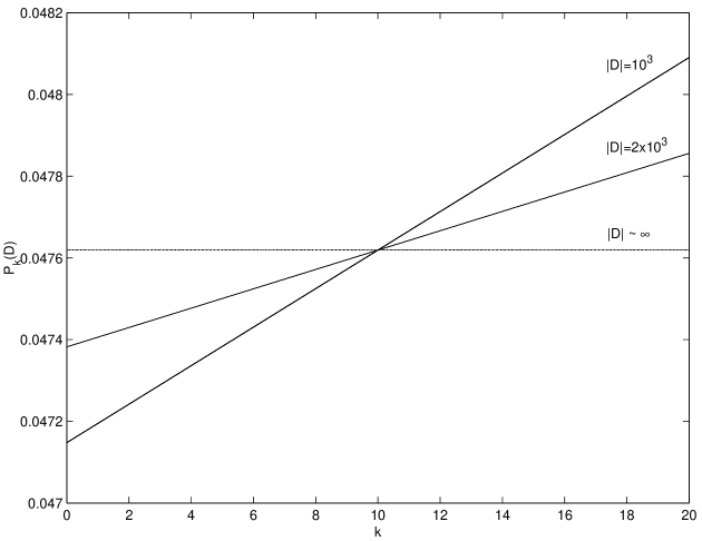
Figure 1: $P_{k}(-1000)$, $P_{k}(-2000)$ and $P_{k}(-\infty)$ for $b_{i}=d_{i}={\rm const}<1$ and $n=20$.

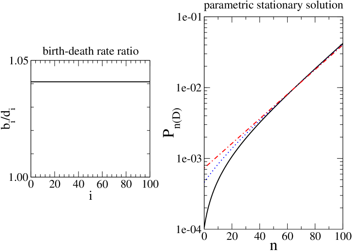
Figure 2: $P_{n}(-4)$ - black straight line; $P_{n}(-40)$ - blue dotted line; $P_{n}(-\infty)$ - red-dotted line, all of them for $\epsilon=0.02$.

Figure 3: Black straight line - $P_{n}(-4)$; blue-dotted line is $P_{n}(-4000)$; red-dotted-dashed line is $P_{n}(-\infty)$- for $b_{i}=0.1+\exp[-0.12\,i]$ and $d_{i}=0.1+\exp[-0.15\,i]$.

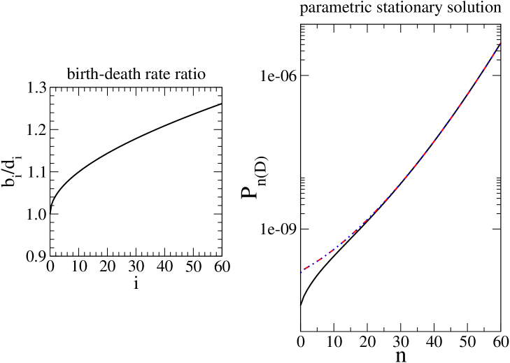
Figure 4: $P_{n}(-4)$ - black straight line; $P_{n}(-4000)$ - blue dotted line; $P_{n}(-\infty)$ - red-dotted line, for $b_{i}=\exp[-0.12\,i^{1/2}]$ and $d_{i}=\exp[-0.15\,i^{1/2}]$.

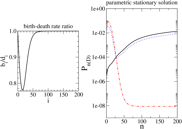
Figure 5: $P_{n}(-4)$ - black straight line; $P_{n}(-4000)$ - blue dotted line; $P_{n}(-\infty)$ - red-dotted line, for $b_{i}=0.01+\exp[-0.15\,i]$ and $d_{i}=0.01+\exp[-0.12\,i]$.

References

- [1] I. Derényi, C. Lee, and A.L. Barabási, Phys. Rev. Lett. 80, 1473 (1998); H.R. Jauslin, Phys. Rev. A 41, 3407 (1990); H.C. Rosu and M. Reyes, Phys. Rev. E 51, 5112 (1995); M.A. Reyes and H.C. Rosu, Nuovo Cimento B 114, 717 (1999).
- [2] I. Volkov, J.R. Banavar, S.P. Hubbell, and A. Maritan, Nature 424, 1035 (2003); A. McKane, D. Alonso, and R.V. Solé, Phys. Rev. E 62, 8466 (2000).
- [3] C.W. Gardiner, Handbook of stochastic methods (Berlin: Springer-Verlag, 1985).
- [4] D.T. Gillespie, Am. J. Phys. 61, 595 (1993).
- [5] B. Mielnik, J. Math. Phys. 25, 3387 (1984).
- [6] See for example, J.A.D. Wattis, J. Phys. A 37, 7823 (2004) and references therein.
- [7] M.R. Geller, Phys. Rev. B 53, 9550 (1996).
- [8] J.J.A. Baselmans, A.F. Morpurgo, B.J. Van Wees, T.M. Klapwijk, Superlattices and Microstructures 25, 973 (1999).