Averaging versus Chaos in Turbulent Transport?

Abstract

In this paper we analyze the transport of passive tracers by deterministic stationary incompressible flows which can be decomposed over an infinite number of spatial scales without separation between them. It appears that a low order dynamical system related to local Peclet numbers can be extracted from these flows and it controls their transport properties. Its analysis shows that these flows are strongly self-averaging and super-diffusive: the delay $\tau(r)$ for any finite number of passive tracers initially close to separate till a distance $r$ is almost surely anomalously fast ($\tau(r)\sim r^{2-\nu}$, with $\nu>0$). This strong self-averaging property is such that the dissipative power of the flow compensates its convective power at every scale. However as the circulation increase in the eddies the transport behavior of the flow may (discontinuously) bifurcate and become ruled by deterministic chaos: the self-averaging property collapses and advection dominates dissipation. When the flow is anisotropic a new formula describing turbulent conductivity is identified.

1 Introduction

In this paper we study the passive transport in $\mathbb{R}^{d}$ ($d\geq 2$) of a scalar $T$ by a divergence free steady vector field $v$ characterized by the following partial differential equation. ($\kappa>0$ being the molecular conductivity)

$$\partial_{t}T+v\nabla T=\kappa\Delta T$$ (1)

We will assume $v$ to be given by an infinite (or large) numbers of spatial scales without any assumption of self-similarity [Ave96]. It will be shown that one can extract from the flow a low order dynamical system related to local Peclet tensors which controls the transport properties of the flow. Based on the analysis of this dynamical system we will show that the transport is almost surely super-diffusive, that is to say, the time of separation of any finite number of passive tracers driven by the same flow and independent thermal noise behave like $r^{2-\nu}$ with $\nu>0$. Similar programs of investigations have shown that the mean squared displacement of a single particle is anomalously fast when averaged with respect to space, time and the randomness of the flow ([Pit97], [KO02], [Fan02]). The point here is to show that the transport is strongly self-averaging: the diffusive properties are anomalously fast (before being averaged with respect to the thermal noise, or a probability law of the flow), moreover the pair separation is also anomalously fast. The fast behavior of the transport of a single particle can be created by long distance correlations in the structure of the velocity field but this is not sufficient to produce fast pair separation. In this paper non-asymptotic estimates will be given, showing that the transport is controlled by a never-ending averaging phenomenon ([Owh01a], [Owh01b], [BO02a], [BO02b]). The analysis of the low order dynamical system allows to obtain a formula linking the minimal and maximal eigenvalues of the turbulent eddy diffusivity. It will be shown that the transport properties depend only on the power law in $v$ and not on its particular geometry (which is not a priori obvious since we consider a quenched model). However, depending on the geometrical characteristics of the eddies at each scale, as the flow rate is increased in these eddies we observe that the super-diffusive behavior may bifurcates towards a Chaotic transport: the multi-scale averaging picture collapses and the flow becomes highly unstable, sensitive to the characteristics of the microstructure and dominated by convective terms.

2 The Model

We want to analyze the properties of the solutions of the following stochastic differential equation which is the Lagrangian formulation of the passive transport equation (1).

$$dy_{t}=\sqrt{2\kappa}d\omega_{t}+\nabla.\Gamma(y_{t})\,dt.$$ (2)

Here $\kappa>0$ is the molecular conductivity of the flow, $\omega_{t}$ a standard Brownian Motion on $\mathbb{R}^{d}$ related to the thermal noise, $\Gamma$ is a skew-symmetric matrix on $\mathbb{R}^{d}$ called stream matrix of the flow and $\nabla.\Gamma$ its divergence. Thus $\nabla.\Gamma$ is the divergence free drift defined by $(\nabla.\Gamma)_{i}=\sum_{j=1}^{d}\partial_{j}\Gamma_{ij}$. We assume that $\Gamma$ is given by an infinite sum of periodic stream matrices with (geometrically) increasing periods and increasing amplitude.

$$\Gamma=\sum_{k=0}^{\infty}\gamma_{k}E^{k}(\frac{x}{R_{k}}).$$ (3)

In the formula (3) we have three important ingredients: the stream matrices $E^{k}$ (also called eddies), the scale parameters $R_{k}$ and the amplitude parameters $\gamma_{k}$ (the stream matrices $E^{k}$ are dimension-less and the parameters $\gamma_{k}$ have the dimension of a conductivity). We will now describe the hypothesis we make on these three items of the model. Let us write $T^{d}:=\mathbb{R}^{d}/\mathbb{Z}^{d}$ the torus of dimension $d$ and side one and for $\alpha\in[0,1]$, $\mathcal{S}^{\alpha}(T^{d})$ the space of $d\times d$ skew-symmetric matrices on $T^{d}$ with $\alpha$-Holder continuous coefficients and $\|.\|_{\alpha}$ the norm associated to that space. For $E\in\mathcal{S}^{\alpha}(T^{d})$

$$\|E\|_{\alpha}:=\sup_{i,j\in\{1,\ldots,d\}}\sup_{x\not=y}|E_{ij}(x)-E_{ij}(y)|/|x-y|^{\alpha}.$$ (4)

1. Hypotheses on the stream matrices $E^{k}$
   There exists $0<\alpha\leq 1$ such that for all $k\in\mathbb{N}$

   $$E^{k}\in\mathcal{S}^{\alpha}(\mathbb{T}^{d}).$$ (5)

   The $\mathcal{S}^{\alpha}$-norm of the $E^{k}$ are uniformly bounded, i.e.

   $$K_{\alpha}:=\sup_{k\in\mathbb{N}}\|E^{k}\|_{\alpha}<\infty.$$ (6)

   Moreover for all $k$,

   $$E^{k}(0)=0.$$ (7)

   Observe that the $\mathcal{S}^{0}$-norms of the $E^{k}$ are uniformly bounded and we will write

   $$K_{0}:=\sup_{k\in\mathbb{N}}\sup_{i,j\in\{1,\ldots,d\}}\|E^{k}\|_{0}$$ (8)

2. Hypotheses on the scale parameters $R_{k}$
   $R_{k}$ is a spatial scale parameter growing exponentially fast with $k$, more precisely we will assume that $R_{0}=r_{0}=1$ and that the ratios between scales defined by

   $$r_{k}=R_{k}/R_{k-1}\in\mathbb{R}^{*}$$ (9)

   for $k\geq 1$, are reals uniformly bounded away from $1$ and $\infty$: we will denote by

   $$\rho_{\min}:=\inf_{k\in\mathbb{N}^{*}}r_{k}\quad\text{and}\quad\rho_{\max}:=\sup_{k\in\mathbb{N}^{*}}r_{k}$$ (10)

   and assume that

   $$\rho_{\min}\geq 2\quad\text{and}\quad\rho_{\max}<\infty.$$ (11)

3. Hypotheses on the flow rates $\gamma_{k}$
   $\gamma_{k}$ is an amplitude parameter (related to the local rate of the flow) growing exponentially fast with the scale $k$, more precisely we will assume that $\gamma_{0}=1$ and that their ratios $\gamma_{k}/\gamma_{k-1}$ for $k\geq 1$, are positive reals uniformly bounded away from $1$ and $\infty$: we will denote by

   $$\gamma_{\min}:=\inf_{k\in\mathbb{N}^{*}}(\gamma_{k}/\gamma_{k-1})\quad\text{and}\quad\gamma_{\max}:=\sup_{k\in\mathbb{N}^{*}}(\gamma_{k}/\gamma_{k-1})$$ (12)

   and assume that

   $$\gamma_{\min}>1\quad\text{and}\quad\gamma_{\max}<\rho_{\min}^{\alpha}.$$ (13)

Remark 2.1.

The uniform $\alpha$-Holder continuity of the stream matrices $E^{k}$ is sufficient to obtain a well defined $\alpha$-Holder continuous stream matrix $\Gamma$, however $\Gamma$ is not differentiable in general. In this case the stochastic differential equation (2) is formal. For the simplicity of the presentation and to start with, when referring to the SDE (2) we will assume that

$$\alpha=1\quad\text{and that the stream matrices $E^{k}$ are uniformly $C^{1}$.}$$ (14)

It follows from the hypothesis I, IIand III   that $\Gamma$ is a well defined uniformly $C^{1}$ skew-symmetric matrix on $\mathbb{R}^{d}$, thus the Stochastic Differential Equation 2 is well defined and admits a unique solution.
The differentiability hypothesis (14) though convenient in order to define the process $y_{t}$ is in fact useless, the theorems are also meaningful and true for $0<\alpha<1$ (since they will refer to the diffusion associated to the weakly defined operator $\nabla.(\kappa+\Gamma)\nabla$).

Remark 2.2.

Observe that the power law of the flow in this paper is not Kolmogorov. Indeed if $v(l)$ is the velocity of the eddies of size $l$ and $\mathcal{E}(k)$ the kinetic energy distribution in the Fourier modes then with the Kolmogorov law one should have

$$v(l)\sim l^{\frac{1}{3}}\quad\text{and}\quad\mathcal{E}(k)\sim k^{-\frac{5}{3}}.$$

In our Model we have

$$v(l)\sim l^{\frac{\ln\gamma}{\ln\rho}-1}\quad\quad\mathcal{E}(k)\sim k^{1-2\frac{\ln\gamma}{\ln\rho}}.$$

Thus to be consistent with a Kolmogorov spectrum one should have $\gamma=\rho^{\frac{4}{3}}$ this case will be analyzed in a forthcoming paper.

As an example, we have illustrated in the figure 1 the contour lines of a two scale flow with stream function $h_{0}^{2}(x,y)=\sum_{k=0}^{2}\gamma^{k}h(\frac{x}{\rho^{k}},\frac{y}{\rho^{k}})$ , with $\rho=3$, $\gamma=1.1$ and $h(x,y)=2\sin(2\pi x+3\cos(2\pi y-3\sin(2\pi x+1)))\sin(2\pi y+3\cos(2\pi x-3\sin(2\pi y+1)))$

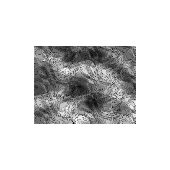
Figure 1: A simple example of the multiscale flow

3 A reminder on the eddy conductivity

We write $\mathcal{M}_{d,{\operatorname{sym}}}$ the space of $d\times d$ symmetric elliptic constant matrices and $\mathcal{S}_{L^{\infty}}(\mathbb{T}^{d}_{R})$ the space of skew-symmetric matrices with coefficients in $L^{\infty}(\mathbb{T}^{d}_{R})$ ($\mathbb{T}^{d}_{R}:=R\mathbb{T}^{d}$ stands for the torus of dimension d and side $R$). For $a\in\mathcal{M}_{d,{\operatorname{sym}}}$ and $E$ a skew symmetric matrix with bounded coefficients the heat kernel associated to the passive transport operator $\nabla.(a+E)\nabla$ (defined in a weak sense) is Gaussian by Aronson estimates [Nor97]. We will now assume $E$ to be periodic: $E\in\mathcal{S}_{L^{\infty}}(\mathbb{T}^{d}_{R})$. In this case the process associated to the operator $L=\nabla.(a+E)\nabla$ exhibits self-averaging properties and we will note $\sigma_{{\operatorname{sym}}}(a,E)$ the effective conductivity associated to the homogenization of that operator [BLP78], [JKO91]. Writing $p(t,x,y)$ the heat kernel associated to $L$, it is well known that $\sigma_{{\operatorname{sym}}}(a,E)$ is a $d\times d$ elliptic symmetric matrix satisfying, for all $x,l\in\mathbb{R}^{d}$

$$|l|^{2}_{\sigma_{{\operatorname{sym}}}(a,E)}=\frac{1}{2}\lim_{t\rightarrow\infty}t^{-1}\int_{\mathbb{R}^{d}}p(t,x,y)(y.l)^{2}\,dy.$$ (15)

We have used the notation $|l|_{a}^{2}:={{}^{t}lal}$. If $z_{t}$ is the process generated by $L$, then as $\epsilon\downarrow 0$, $\epsilon z_{t/{\epsilon^{2}}}$ converges in law to a Brownian motion with covariance matrix $D(a,E)$ called effective diffusivity and proportional to the effective conductivity.

$$D(a,E)=2\sigma_{{\operatorname{sym}}}(a,E).$$ (16)

Let us remind that $\sigma_{{\operatorname{sym}}}(a,E)$ is given by the following variational formula ([Nor97] lemma 3.1): for $\xi\in\mathbb{R}^{d}$

$$|\xi|_{\sigma_{{\operatorname{sym}}}^{-1}(a,E)}^{2}=\inf_{(f,H)\in C^{\infty}(\mathbb{T}^{d}_{R})\times\mathcal{S}(\mathbb{T}^{d}_{R})}R^{-d}\int_{\mathbb{T}^{d}_{R}}|\xi-\nabla.H+(a+E)\nabla f|_{a^{-1}}^{2}\,dx.$$ (17)

Where we have written $\mathcal{S}(\mathbb{T}^{d}_{R})$ the space of skew symmetric matrices with coefficients in $C^{\infty}(\mathbb{T}^{d}_{R})$.
The symmetric tensor $\sigma_{{\operatorname{sym}}}(a,E)$ is also called eddy conductivity: after averaging the information on particular geometry of the eddies associated to $E$ is lost and the conductivity of the flow is replaced by an increased conductivity $\sigma_{{\operatorname{sym}}}(a,E)$. Let us define for $P\in\mathcal{S}_{L^{\infty}}(\mathbb{T}^{d})$ and $\rho\in\mathbb{R}^{*}$, $S_{\rho}P\in\mathcal{S}_{L^{\infty}}(\mathbb{T}^{d}_{\frac{1}{\rho}})$ by

$$S_{\rho}P(x):=P(\rho x).$$ (18)

It is important to note that the effective conductivity is invariant by scaling, i.e. $\sigma_{{\operatorname{sym}}}(a,S_{\rho}P)=\sigma_{{\operatorname{sym}}}(a,P)$; thus we can assume for simplicity that $R=1$ and $E\in\mathcal{S}_{L^{\infty}}(\mathbb{T}^{d})$. When $E$ is smooth $\sigma_{{\operatorname{sym}}}(a,E)$ is given [BLP78] by solving the following cell problem:

$$\nabla.(a+E)(l-\nabla\chi_{l}^{a,E})=0.$$ (19)

Where $l\in\mathbb{R}^{d}$, $\chi_{l}^{a,E}\in C^{\infty}(\mathbb{T}^{d})$ and $\int_{\mathbb{T}^{d}}\chi_{l}^{a,E}(x)\,dx=0$. Write $F_{l}^{a,E}=l.x-\chi_{l}^{a,E}(x)$, observe that $F_{l}^{a,E}$ is linear in $l$, thus we will write $F^{a,E}$ the vector field $(F^{a,E})_{i}:=F_{e_{i}}^{a,E}$ and $\nabla F^{a,E}$ the matrix $(\nabla F^{a,E})_{ij}:=\partial_{i}F^{a,E}_{e_{j}}$. The eddy conductivity is then given by

$$\sigma_{{\operatorname{sym}}}(a,E)=\int_{\mathbb{T}^{d}}{{}^{t}\nabla F^{a,E}(x)a\nabla F^{a,E}(x)}\,dx.$$ (20)

Let us remind that the matrix $\sigma(a,E)$ defined by

$$\sigma(a,E):=\int_{\mathbb{T}^{d}}(a+E(x))\nabla F^{a,E}(x)\,dx$$ (21)

is called the flow effective conductivity [FP94] and is also given by the following variational formula [Nor97]: for $\xi,l\in\mathbb{R}^{d}$

$$\begin{split}|\xi-\sigma(a,E)l|_{\sigma_{sym}^{-1}(a,E)}^{2}:=\inf_{(f,H)\in C^{\infty}(\mathbb{T}^{d})\times\mathcal{S}(\mathbb{T}^{d})}\int_{\mathbb{T}^{d}}|\xi-\nabla.H-(a+E)(l-\nabla f)|_{a^{-1}}^{2}\,dx.\end{split}$$ (22)

It is easy to check that $\sigma_{{\operatorname{sym}}}(a,E)$ is the symmetric part of $\sigma(a,E)$ which implies the following variational formulation for the eddy conductivity

$$|l|_{\sigma_{{\operatorname{sym}}}}^{2}=\inf_{\xi\perp l,(f,H)\in C^{\infty}(\mathbb{T}^{d})\times\mathcal{S}(\mathbb{T}^{d})}\int_{\mathbb{T}^{d}}|\xi-\nabla.H-(a+E)(l-\nabla f)|^{2}_{a^{-1}}\,dx.$$ (23)

Where we have written $\xi\perp l$ is the subspace of $\xi\in\mathbb{R}^{d}$ orthogonal to the vector $l$: $\xi.l=0$.

4 Main results

4.1 Averaging with two scales

Let $a\in\mathcal{M}_{d,{\operatorname{sym}}}$, $P\in\mathcal{S}_{L^{\infty}}(\mathbb{T}^{d})$ and $K\in\mathcal{S}^{\alpha}(\mathbb{T}^{d})$. We will prove in subsection 5.1 the following estimate of $\sigma_{{\operatorname{sym}}}(a,S_{R}P+K)$ the effective conductivity for a two-scale medium when $R$ is an integer (and $S_{R}$ is the scaling operator (18)).

Theorem 4.1.

There exists a function $f:\mathbb{R}^{2}\rightarrow\mathbb{R}^{+}$ increasing in each of its arguments such that for $a\in\mathcal{M}_{d,{\operatorname{sym}}}$, $R\in\mathbb{N}^{*}$, $P\in\mathcal{S}_{L^{\infty}}(\mathbb{T}^{d})$ and $K\in\mathcal{S}^{\alpha}(\mathbb{T}^{d})$

$$\begin{split}\left(1+\epsilon\left(R\right)\right)^{-4}\sigma_{{\operatorname{sym}}}\big{(}\sigma_{{\operatorname{sym}}}(a,P),K\big{)}\leq\sigma_{{\operatorname{sym}}}(a,S_{R}P+K)\leq\sigma_{{\operatorname{sym}}}\big{(}\sigma_{{\operatorname{sym}}}(a,P),K\big{)}(1+\epsilon(R))^{4}.\end{split}$$ (24)

$$\begin{split}\text{With}\quad\epsilon(R)=\big{(}\frac{\|K\|_{\alpha}}{R^{\alpha}\lambda_{\min}(a)}\big{)}^{\frac{1}{2}}f(d,\frac{\|a+P\|_{\infty}}{\lambda_{\min}(a)}).\end{split}$$ (25)

Remark 4.2.

Theorem 4.1 implies obviously that

$$\begin{split}\sigma_{{\operatorname{sym}}}\big{(}\sigma_{{\operatorname{sym}}}(a,P),K\big{)}=\lim_{R\rightarrow\infty}\sigma_{{\operatorname{sym}}}(a,S_{R}P+K).\end{split}$$ (26)

Thus $\sigma_{{\operatorname{sym}}}\big{(}\sigma_{{\operatorname{sym}}}(a,P),K\big{)}$ should be interpreted as the effective conductivity of the two-scale flow with a complete separation of scales. So we will also write it $\sigma_{{\operatorname{sym}}}(a,S_{\infty}P+K)$. Naturally $\sigma_{{\operatorname{sym}}}\big{(}\sigma_{{\operatorname{sym}}}(a,P),K\big{)}$ is also computable from an explicit cell problem (see (20)).

Averaging versus chaotic coupling

The equation (24) basically says that when $\epsilon(R)$ is small, the mixing length of the smaller scale $P(Rx)$ is smaller than scale at which the fluctuations of the larger scale $K(x)$ start to be felt. Now it is very important to observe that as $\lambda_{\min}(a)\downarrow 0$, $\epsilon(R)$ explode towards infinity and this collapse of the two-scale averaging is not an artefact, it is easy to see that the estimate (25) is sharp. What happens is a transition from averaging to a chaotic coupling between the two scales. More precisely as $\lambda_{\min}(a)\downarrow 0$, the mixing length of the smaller scale explode well above the visibility length of the larger scale, the two scales are no longer separated in the averaging and their particular geometry can no longer be ignored (collapse of the averaging paradigm). Moreover writing for $y\in[0,1]^{d}$, $\Theta_{y}$ the translation operator acting on functions $f$ of $\mathbb{R}^{d}$ by $\Theta_{y}f(x)=f(x+y)$, observe that in the limit of complete separation between scales the two-scale averaging is invariant with respect to a relative translation of one scale with respect to an other:

$$\begin{split}\lim_{R\rightarrow\infty}\sigma_{{\operatorname{sym}}}(a,S_{R}\Theta_{y}P+K)=\lim_{R\rightarrow\infty}\sigma_{{\operatorname{sym}}}(a,S_{R}P+K).\end{split}$$ (27)

But the limit $\lambda_{\min}(a)\downarrow 0$ is singular and this invariance by translation is lost: for $l\in\mathbb{R}^{d}$

$$\begin{split}\Big{(}{{}^{t}l}\sigma_{{\operatorname{sym}}}(a,S_{R}\Theta_{y}P+K)l-{{}^{t}l}\sigma_{{\operatorname{sym}}}(a,S_{R}P+K)l\Big{)}\Big{(}{{}^{t}l}\sigma_{{\operatorname{sym}}}(a,S_{R}P+K)l\Big{)}^{-1}.\end{split}$$ (28)

may explode towards infinity. Indeed it is easy to see that for any $R\in\mathbb{N}^{*}$, there exist $P,K\in\mathcal{S}^{1}(\mathbb{T}^{d})$ with $\|P\|_{1}\leq C_{d}$, $\|K_{1}\|\leq C_{d}$ such that there exists $y\in[0,1]^{d}$ and $l\in\mathbb{R}^{d}$ with

$$\begin{split}\lim_{\zeta\downarrow 0}\Big{(}{{}^{t}l}\sigma_{{\operatorname{sym}}}(\zeta I_{d},S_{R}\Theta_{y}P+K)l\Big{)}\Big{(}{{}^{t}l}\sigma_{{\operatorname{sym}}}(a,S_{R}P+K)l\Big{)}^{-1}=\infty.\end{split}$$ (29)

We have illustrated this symmetry breaking in the figures 2 representing a two scale flow. In figure 2(a) the larger eddies are surrounded by a non void region where the flow is null and asymptotic behavior of the effective conductivity at vanishing molecular conductivity is given by

$$\begin{split}\sigma_{{\operatorname{sym}}}(\zeta I_{d},S_{R}P+K)\sim C_{1}\zeta I_{d}.\end{split}$$ (30)

In figure 2(b) we have operated a small translation of the smaller scale with respect to the larger one. The result of this relative translation is the percolation of stream lines of the flow: a particle driven by the flow can go to infinity by following them. It follows after this small perturbation that asymptotic behavior of the effective conductivity of the two scale flow at vanishing molecular conductivity is given by

(31).

$$\begin{split}\sigma_{{\operatorname{sym}}}(\zeta I_{d},S_{R}\Theta_{y}P+K)\sim C_{2}\zeta^{\frac{1}{2}}I_{d}.\end{split}$$ (31)

We call this sensibility with respect to the relative translation $\Theta_{y}$, chaotic coupling between scales.

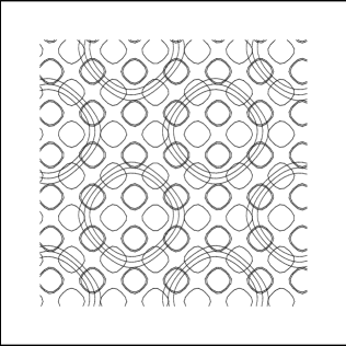
(a) stream lines of $S_{R}P$ and $K$.

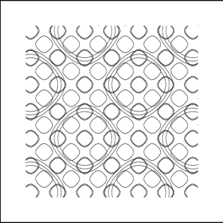
(b) stream lines of $S_{R}\Theta_{y}P$ and $K$.

Figure 2: Two scales flow.

The asymptotic (31) can be understood from a boundary layer analysis (see [Chi79] and [FP94]).

4.2 Multiscale eddy conductivity and the renormalization core.

Let us write

$$\Gamma^{0,n}=\sum_{k=0}^{n}\gamma_{k}E^{k}(\frac{x}{R_{k}}).$$ (32)

For this subsection we will use the following hypothesis

IV

Hypothesis on the ratios between scales: for all $k\in\mathbb{N}$, $r_{k}\in\mathbb{N}^{*}$.

Our objective is to obtain quantitative estimates the multi-scale eddy viscosities $\big{(}\sigma(\Gamma^{0,n})\big{)}_{n\in\mathbb{N}}$; observe that under the hypothesis IV, $\Gamma^{0,n}$ is periodic, thus its effective conductivity is well defined by equation (17) (that is its only utility, we will not need this hypothesis to prove super-diffusion). These estimates (theorem 4.4) will be proven by induction on the number of scales. The basic step in this induction is the estimate (24) on the effective conductivity for a two scale periodic medium. We will need to introduce a dynamical system called the renormalization core which will play a central role in the transport properties of the stochastic differential equation (2).

Definition 4.3.

We propose to call ”renormalization core” the dynamical system $(A^{n})_{n\in\mathbb{N}}$ of $d\times d$ symmetric strictly elliptic matrices defined by

$$A^{0}=\frac{\kappa}{\gamma_{0}}I_{d}\quad\text{and}\quad A^{n+1}=\frac{\gamma_{n}}{\gamma_{n+1}}\sigma_{sym}(A^{n},E^{n}).$$ (33)

For $B$ a $d\times d$ symmetric coercive matrix let us define the function $g(B)$ by

$$g(B):=\big{(}\frac{K_{\alpha}}{\lambda_{\min}(B)(1-\gamma_{\max}/\rho_{\min}^{\alpha})}\big{)}^{\frac{1}{2}}f\big{(}d,(\lambda_{\max}(B)+K_{0})/\lambda_{\min}(B)\big{)}.$$ (34)

Where $f$ is the function appearing in theorem 4.1. We will prove in the subsection 5.2 the following theorem.

Theorem 4.4.

Under hypotheses I, II, IIIand IVfor all $n\in\mathbb{N}^{*}$

$$\begin{split}\gamma_{n+1}A^{n+1}\prod_{p=1}^{n}(1+\epsilon_{p})^{-4}\leq\sigma_{sym}(\kappa I_{d},\Gamma^{0,n})\leq\gamma_{n+1}A^{n+1}\prod_{p=1}^{n}(1+\epsilon_{p})^{4}\end{split}$$ (35)

with

$$\epsilon_{p}=\Big{(}\frac{\gamma_{p}}{\gamma_{p-1}r_{p}^{\alpha}}\Big{)}^{\frac{1}{2}}g(A^{p-1}).$$ (36)

$A^{n}$ being the renormalization core (33)

Observe that $\gamma_{n+1}A^{n+1}$ is the etimate given by reiterated homogenization under the assumption of complete separation between scales, i.e. $\rho_{\min}\rightarrow\infty$ and the error term $\prod_{p=1}^{n}(1+\epsilon_{p})^{4}$ controlled by the renormalization core $A^{k}$ which reflects the interaction between the scales $k$ and $k+1$. As $\lambda_{\min}(A_{k})\downarrow 0$ one passes from a separation of the scales $k$ and $k+1$ to a chaotic coupling between this two scales. Moreover it is easy to obtain from theorem 4.4 that

$$\lim_{r_{1},\ldots,r_{n-2}\rightarrow\infty}\sigma_{sym}(\kappa I_{d},\Gamma^{0,n})=\gamma_{n-1}\sigma_{sym}(A^{n-1},S_{r_{n}}E^{n-1}+\frac{\gamma_{n}}{\gamma_{n-1}}E^{n}).$$ (37)

Assume that the multi-scale averaging scenario holds and $\rho_{\min}<\infty$. In that scenario, $\sigma_{sym}(\kappa I_{d},\Gamma^{0,n})$ can be approximated by its limit at asymptotic separation between scales. We obtain a contradiction if $\liminf_{n\rightarrow\infty}\lambda_{\min}(A^{n})=0$ from (37) and the collapse of the two-scale averaging scenario given in subsection 4.1 and figure 2. In other words if $\liminf_{n\rightarrow\infty}\lambda_{\min}(A^{n})=0$ then the self-averaging property of the flow collapses towards a chaotic coupling between all the scales which is characterized by the breaking of the invariance by relative translation between the scales.

4.2.1 What is the renormalization core?

First observe that it is a dimensionless tensor. At the limit of infinite separation between scales the eddy conductivity created by the scales $0,\ldots,n-1$ is $\lim_{\rho_{\min}\rightarrow\infty}\sigma_{{\operatorname{sym}}}(\kappa I_{d},\Gamma^{0,n-1})$. The typical scale length associated to the scale $n$ is $R_{n}$ and the velocity of the flow at this scale is of the order of $\gamma_{n}R_{n}^{-1}$ (we assume $K_{1}$ to be of order one). Thus at the scale $n$ one can define a local renormalized Peclet tensor $\bf{Pe}^{n}$ by:

$$\bf{Pe}^{n}:=R_{n}\times\frac{\gamma_{n}}{R_{n}}\times\big{(}\lim_{\rho_{\min}\rightarrow\infty}\sigma_{{\operatorname{sym}}}(\kappa I_{d},\Gamma^{0,n-1})\big{)}^{-1}.$$ (38)

But at the limit of complete separation between scales $(A^{n})^{-1}$ is equal to the ratio between the convective strength $\gamma_{n}$ of the scale $n$ and the local turbulent conductivity at the scale $n-1$:

$$(A^{n})^{-1}=\lim_{\rho_{\min}\rightarrow\infty}\gamma_{n}\big{(}\sigma_{{\operatorname{sym}}}(\kappa I_{d},\Gamma^{0,n-1})\big{)}^{-1}.$$ (39)

It follows that

$$(A^{n})^{-1}=\bf{Pe}^{n}.$$ (40)

Thus one can interpret the renormalization core as the inverse of the Peclet tensor of the flow at the scale $n$ assuming that all the smaller scales have been completely averaged.

Definition 4.5.

We call ”local renormalized Peclet tensor” $(\bf{Pe}^{n})_{n\in\mathbb{N}}$ the inverse of the renormalization core

$$\bf{Pe}^{n}=(A^{n})^{-1}.$$ (41)

4.2.2 Pathologies of the renormalization core.

Definition 4.6.

We call stability of the renormalization core (33) the sequence

$$\lambda^{-}_{n}:=\inf_{0\leq p\leq n}\lambda_{\min}(A^{p}).$$ (42)

We write

$$\lambda^{-}_{\infty}:=\lim_{n\rightarrow\infty}\lambda^{-}_{n}\quad\text{and}\quad\lambda^{-}:=\liminf_{n\rightarrow\infty}\lambda_{\min}(A^{n}).$$ (43)

The renormalization core is said to be stable if and only if $\lambda^{-}>0$.

Definition 4.7.

We call anisotropic distortion of the renormalization core (33) the sequence

$$\mu_{n}=\sup_{0\leq p\leq n}\big{(}\lambda_{\max}(A^{p})/\lambda_{\min}(A^{p})\big{)}.$$ (44)

We write

$$\mu_{\infty}:=\lim_{n\rightarrow\infty}\mu_{n}\quad\text{and}\quad\mu:=\limsup_{n\rightarrow\infty}\big{(}\lambda_{\max}(A^{n})/\lambda_{\min}(A^{n})\big{)}.$$ (45)

The renormalization core (33) is said to have unbounded (bounded) anisotropic distortion if and only if $\mu=\infty$ ($\mu<\infty$).

Definition 4.8.

We call ubiety of the renormalization core (33) the sequence

$$\lambda^{+}_{n}:=\sup_{0\leq p\leq n}\lambda_{\max}(A^{p}).$$ (46)

We write

$$\lambda^{+}_{\infty}:=\lim_{n\rightarrow\infty}\lambda^{+}_{n}\quad\text{and}\quad\lambda^{+}:=\limsup_{n\rightarrow\infty}\lambda_{\max}(A^{n}).$$ (47)

The renormalization core is said to be vanishing if and only if $\lambda^{+}=0$

Definition 4.9.

The renormalization core (33) is said to be bounded if and only if $\lambda^{+}<\infty$.

The renormalization core is gifted with remarkable properties which will be analyzed in details in subsection 4.4. Before proceeding to super-diffusion we will give a first theorem stressing the role of the stability of the renormalization core, that is to say the fact that the local renormalized Peclet tensor stays bounded away from infinity. Indeed, it follows from theorem 4.4 that the averaging paradigm for our model is valid if the renormalization core is stable, and has bounded anisotropic distortion. We may naturally wonder whether the fact that the local renormalized Peclet tensor stays bounded away from infinity is sufficient, the answer is positive as shown by the following theorem which will be proven in subsection 5.3.

Theorem 4.10.

Writing $C=C_{d}K_{0}^{2}(1-1/\gamma_{\min})^{-1}$ we have

1. If the renormalization core is not bounded ($\lambda^{+}=\infty$) then it is not stable ($\lambda^{-}=0$)

2. If the renormalization core is stable ($\lambda^{-}>0$) then it is bounded and

   $$\lambda^{+}\leq\frac{C}{\lambda^{-}}.$$ (48)

3. The renormalization core has unbounded anisotropic distortion ($\mu=\infty$) if and only if it is not stable ($\lambda^{-}=0$)

4. If the renormalization core is stable ($\lambda^{-}>0$) then it has bounded anisotropic distortion ($\mu<\infty$) and

   $$\mu\leq\frac{C}{(\lambda^{-})^{2}}.$$ (49)

Combining theorem 4.10 and 4.4 we obtain that if the renormalization core is stable then the local turbulent eddy conductivity diverges towards infinity like $\gamma_{n}$ independently of the geometry of the eddies (if it is not stable the behavior of the local turbulent eddy conductivity depends on the geometry of the eddies ). More precisely we have the following theorem.

Theorem 4.11.

Under hypotheses I, II, IIIand IV, if the renormalization core is stable then there exists $C$ such that for $\rho_{\min}^{\alpha}>C\gamma_{\max}$ one has

$$\begin{split}\limsup_{n\rightarrow\infty}\frac{\ln\Big{(}\lambda_{\max}\big{(}\sigma_{sym}(\kappa I_{d},\Gamma^{0,n})\big{)}\Big{)}}{\ln\gamma_{n}}\leq 1+\epsilon\end{split}$$ (50)

and

$$\begin{split}\liminf_{n\rightarrow\infty}\frac{\ln\Big{(}\lambda_{\min}\big{(}\sigma_{sym}(\kappa I_{d},\Gamma^{0,n})\big{)}\Big{)}}{\ln\gamma_{n}}\geq 1-\epsilon\end{split}$$ (51)

with $\epsilon:=0.5\big{(}C\gamma_{\max}/(\rho_{\min})\big{)}^{\frac{1}{2}}<0.5$ and $C:=K_{\alpha}h(d,K_{0}/\lambda^{-})$. $h$ being a finite increasing positive function in each of its arguments.

Remark 4.12.

For a real flow, call $\sigma(r)$ the local turbulent diffusivity of the flow at the scale $r$ and $v(r)$ the magnitude of the vector velocity field at that scale then the key relation implying that the distortions created at the scale $r$ are dissipated by the mixing power of the smaller scales is the relation

$$\sigma(r)\sim rv(r)$$ (52)

This relation is at the core of the Kolmogorov (K41) analysis and the analysis of fully developed turbulence by Landau-Lifschitz [LL84]. The result given in Theorem 4.11 corresponds to the relation (52) obtained and used from a heuristic point of view (dimension analysis) by physicists.

4.3 Super-diffusion

Anomalous fast exit times

We write $\tau(r)$ the exit time of the process $y_{t}$ (2) from the ball $B(0,r)$. We write $\mathbb{E}_{x}$ the expectation associated to the process $y_{t}$ started from the point $x$. We write ${\operatorname{Vol}}\big{(}B(0,r)\big{)}$ the Lebesgue measure of $B(0,r)$. We define $n(r)$ as the number of (smaller) scales which will be considered as averaged at the scale $r$.

$$n(r):=\sup\{p\in\mathbb{N}\,:\,R_{p}\leq r\}.$$ (53)

Let $m_{r}$ be the Lebesgue probability measure on the ball $B(0,r)$ defined by

$$m_{r}(dx):=\frac{dx}{\int_{B(0,r)}dx}1_{B(0,r)}.$$ (54)

We will consider the mean exit time for the process started with initial distribution $m_{r}$, i.e.

$$\begin{split}\mathbb{E}_{m_{r}}\big{[}\tau(r)\big{]}=\frac{1}{{\operatorname{Vol}}\big{(}B(0,r)\big{)}}\int_{B(0,r)}\mathbb{E}_{x}\big{[}\tau(r)\big{]}\,dx.\end{split}$$ (55)

We will prove in subsection 5.4 the following theorem.

Theorem 4.13.

Under hypotheses I, II, and IIIwith $\alpha=1$, if the renormalization core is stable ($\lambda^{-}>0$) then there exists a constant $Q$ such that for $\rho_{\min}>Q\gamma_{\max}$ one has

$$\begin{split}\limsup_{r\rightarrow\infty}\frac{1}{\ln r}\ln\Big{(}\mathbb{E}_{m_{r}}\big{[}\tau(r)\big{]}\Big{)}<2.\end{split}$$ (56)

More precisely for $r>R_{1}$ one has

$$\begin{split}\mathbb{E}_{m_{r}}\big{[}\tau(r)\big{]}=r^{2-\nu(r)}\end{split}$$ (57)

with

$$\nu(r)=\frac{\ln\gamma_{n(r)}}{\ln r}\big{(}1+\epsilon(r)\big{)}+\frac{C(r)}{\ln r}.$$ (58)

and $|C(r)|\leq C(d,K_{0},\gamma_{\max})+|\ln\lambda^{-}_{\infty}|$,

$$|\epsilon(r)|<0.5\big{(}\frac{Q\gamma_{\max}}{\rho_{\min}}\big{)}^{\frac{1}{2}}\leq 0.5$$ (59)

and there exists a finite increasing positive function in each of its arguments $F$ such that

$$Q:=\frac{1}{(\ln\gamma_{\min})^{2}}F\big{(}d,\frac{(1+K_{0})^{2}(1-1/\gamma_{\min})^{-1}+\kappa}{\lambda^{-}_{\infty}}\big{)}(1+K_{1}).$$ (60)

Remark 4.14.

Equation (58) shows that the anomalous constant is directly related to the number of effective scales. Observe that

$$\nu(r)\leq\frac{\ln\gamma_{\max}}{\ln\rho_{\min}}\Big{(}1+0.5\big{(}\frac{Q\gamma_{\max}}{\rho_{\min}}\big{)}^{\frac{1}{2}}\Big{)}+\frac{C(d,K_{0},\gamma_{\max})}{\ln r}$$ (61)

and

$$\nu(r)\geq\frac{\ln\gamma_{\min}}{\ln\rho_{\max}}\Big{(}1-0.5\big{(}\frac{Q\gamma_{\max}}{\rho_{\min}}\big{)}^{\frac{1}{2}}\Big{)}-\frac{C(d,K_{0},\gamma_{\max})}{\ln r}$$ (62)

and $\nu(r)>0.4(\ln\gamma_{\min}/\ln\rho_{\max})$ for $r$ large enough. The anomalous parameter $\nu(r)$ is not a constant because the model is not self-similar, in a self similar case ($\gamma_{\min}=\gamma_{\max}=\gamma$ and $\rho_{\min}=\rho_{\max}=\rho$) one would have at a logarithmic approximation

$$\mathbb{E}[\tau(r)]\sim r^{2-\nu}\quad\text{with}\quad\nu\sim\frac{\ln\gamma}{\ln\rho}.$$

The error terms in $\nu(r)$ are explained by the interaction between the scales which are sensitive to the particular geometry of the eddies. We remind that we consider a quenched model and it is not a priori obvious that the transport should depend only on the power law in velocity field and not on its particular geometry.

Sufficient (and necessary) conditions for the stability of the renormalization core ($\lambda^{-}>0$) will be given in subsection 4.4; we refer to theorems 4.25, 4.26 and 4.30. In particular if $d=2$ and if for all $k$, $E^{k}=E$ where $E$ corresponds to the cellular flow ($E_{12}(x,y):=\sin(2\pi x)\cos(2\pi y)$) then the renormalization core is stable ($\lambda^{-}>0$). We have illustrated the contour lines of the superposition of $4$ scales of cellular flows in figure 3.

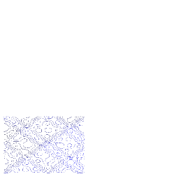
Figure 3: Superposition of cellular flows.

There exists an important literature on the fast transport phenomenon in turbulence addressed (from both heuristic and rigorous point of view) by using the tools of homogenization or renormalization; we refer to [KS79], [AM90], [AM87], [FGL⁺91], [GLPP92], [GZ92], [Zha92], [GK98], [IK91], [Gau98], [Ave96], [Bha99], [FK01], [BO02b], [CP01], [AC02] and this panorama is far from being complete, we refer to [MK99] and [Woy00] for a survey.
For non exactly solvable models (non shear flows) asymptotic fast scaling in the transport behavior have been obtained in the framework of spectral averaging in turbulence. Along this axis L. Piterbarg has obtained [Pit97] fast asymptotic scaling after averaging the transport with respect to the law of the velocity field and the thermal noise and rescaling with respect to space and time. More recently S. Olla and T. Komorowski [KO02] have observed the asymptotic anomalously fast behavior of the mean squared displacement averaged with respect to the thermal noise, the law of the velocity field and time. A. Fannjiang [Fan02] has studied a model where the law of separation of two particles is postulated to be the transport law of a single one as studied in [KO02] and [Pit97].

Fast mixing.

In order to show that the phenomenon presented in theorem 4.13 is super-diffusion and not mere convection, we must compute the rate at which particles do separate and show that this rate follows the same fast behavior. More precisely we will consider $(y_{t},z_{t})\in\mathbb{R}^{d}\times\mathbb{R}^{d}$ where $y_{t}$ is the solution of (2) and $z_{t}$ follows the following stochastic differential equation

$$dz_{t}=\sqrt{2\kappa}d\bar{\omega}_{t}+\nabla.\Gamma(z_{t})\,dt.$$ (63)

Where $\bar{\omega}_{t}$ is a standard Brownian motion independent of $\omega_{t}$. Thus $y_{t}$ and $z_{t}$ can be seen as two particles transported by the same drift but with independent identically distributed noise. Let us write $B(0,r,l)$ the following subset of $\mathbb{R}^{d}\times\mathbb{R}^{d}$

$$B(0,r,l):=\big{\{}(y,z)\in\mathbb{R}^{d}\times\mathbb{R}^{d}\,:\,|y-z|<r\quad\text{and}\quad y^{2}+z^{2}<l^{2}\big{\}}.$$ (64)

We write $\mathbb{E}_{y,z}\big{[}\tau(r,l)\big{]}$ the expectation of the exit time of the diffusion $(y_{t},z_{t})$ from $B(0,r,l)$ with $(y_{0},z_{0})=(y,z)$. Let $m_{r,l}$ be the Lebesgue probability measure on the set $B(0,r,l)$ defined by

$$m_{r,l}(dy\,dz):=\frac{dy\,dz}{\int_{(y,z)\in B(0,r,l)}dy\,dz}1_{B(0,r,l)}.$$ (65)

We will consider the mean exit time for the process $(y_{t},z_{t})$ started with initial distribution $m_{r,l}$, i.e.

$$\begin{split}\mathbb{E}_{m_{r,l}}\big{[}\tau(r,l)\big{]}=\frac{1}{{\operatorname{Vol}}\big{(}B(0,r,l)\big{)}}\int_{B(0,r,l)}\mathbb{E}_{y,z}\big{[}\tau(r,l)\big{]}\,dx.\end{split}$$ (66)

We have the following theorem proven in subsection 5.4.

Theorem 4.15.

Under hypotheses I, II, and IIIwith $\alpha=1$, if the renormalization core is stable then there exists a constant $Q$ such that for $\rho_{\min}>Q\gamma_{\max}$ one has

$$\begin{split}\limsup_{r\rightarrow\infty}\lim_{l\rightarrow\infty}\frac{1}{\ln r}\ln\Big{(}\mathbb{E}_{m_{r,l}}\big{[}\tau(r,l)\big{]}\Big{)}<2.\end{split}$$ (67)

More precisely for $r>R_{1}$ one has

$$\begin{split}\lim_{l\rightarrow\infty}\mathbb{E}_{m_{r,l}}\big{[}\tau(r,l)\big{]}=r^{2-\nu(r)}.\end{split}$$ (68)

where $\nu(r)$ is given by (58) and $Q$ by (60).

Remark 4.16.

It is easy to extend this theorem to any finite number of particles driven by the same flow but independent thermal noise.

Strong self-averaging property.

A trivial consequence of theorem 4.13 and 4.15 is the fact that fast mixing is an almost sure event. More precisely, let us write $H(r)$ and $H(r,l)$ the events

$$H(r):=\Big{\{}\tau(r)\leq r^{2-\delta}\Big{\}}\quad\text{and}\quad H(r,l):=\Big{\{}\tau(r,l)\leq r^{2-\delta}\Big{\}}$$

with $\delta=0.9\ln\gamma_{\min}/\ln\rho_{\max}$. Observe that $\delta>0$ and we have the following theorem

Theorem 4.17.

Under hypotheses I, IIand IIIwith $\alpha=1$, if the renormalization core is stable then there exists a constant $Q$ such that for $\rho_{\min}>Q\gamma_{\max}$ one has

$$\lim_{r\rightarrow\infty}\mathbb{P}_{m_{r}}\big{[}H(r)\big{]}=1\quad\text{and}\quad\lim_{r\rightarrow\infty}\lim_{l\rightarrow\infty}\mathbb{P}_{m_{r,l}}\big{[}H(r,l)\big{]}=1.$$ (69)

In this theorem $Q$ is given by (60), by slightly modifying the constants.

4.4 Diagnosis of renormalization core’s pathologies

With subsection 4.3 we have seen that our model is super-diffusive if the renormalization core is stable. With this subsection we will give necessary and sufficient conditions for the stability of the renormalization core by analyzing in details its dynamic. The results given here will be proven in subsection 5.3.

Diffusive properties of the eddies at vanishing molecular conductivity.

We will need the following functions $V$ and $W$ describing the effective behavior of the eddies $E^{k}$ of the renormalization core at vanishing molecular conductivity. For $E\in\mathcal{S}_{L^{\infty}}(\mathbb{T}^{d})$ and $\zeta>0$ we write

$$V(\zeta,E):=\frac{\lambda_{\min}\big{(}\sigma_{{\operatorname{sym}}}(\zeta I_{d},E)\big{)}}{\zeta}.$$ (70)

Observe that by the variational formulation (17) one has

$$1/V(\zeta,E)=\sup_{\xi\in\mathbb{S}^{d-1}}\inf_{(f,H)\in C^{\infty}(\mathbb{T}^{d})\times\mathcal{S}(\mathbb{T}^{d})}\int_{\mathbb{T}^{d}}|\xi-\nabla.H+E\nabla f|^{2}\,dx+\zeta^{2}\int_{\mathbb{T}^{d}}|\nabla f(x)|^{2}\,dx.$$ (71)

Where we have written $\mathbb{S}^{d-1}$ the unit sphere of $\mathbb{R}^{d}$ centered on $0$. Observe that if for $\xi\in\mathbb{S}^{d-1}$, $\nabla.E.\xi\not\equiv 0$ one has $\forall\zeta>0$ $V(\zeta,E)>1$. Moreover $V$ is continuous and decreasing in $\zeta$. Let us define

Definition 4.18.

$$V(\zeta):=\inf_{n\in\mathbb{N}}V(\zeta,E^{n})$$ (72)

$$V(0):=\lim_{\zeta\downarrow 0}V(\zeta)$$ (73)

Observe that $V(\zeta)$ is a decreasing function in $\zeta$ thus the limit (73) is well defined and belongs to $[1,\infty]$. We define for $x\in\big{(}1,V(0)\big{)}$, the inverse function $V^{-1}$ as

$$V^{-1}(x):=\sup\{y>0\,:\,V(y)>x\}.$$ (74)

Observe that if $V(0)>1$, $V^{-1}(x)$ is a decreasing function of $x$ in $\big{(}1,V(0)\big{)}$.
Similarly we introduce

$$W(\zeta,E):=\frac{\lambda_{\max}\big{(}\sigma_{{\operatorname{sym}}}(\zeta I_{d},E)\big{)}}{\zeta}.$$ (75)

Observe that by the variational formulation (23) one has

$$W(\zeta,E)=1+\sup_{l\in\mathcal{S}^{d-1}}\inf_{\xi\perp l,(f,H)\in C^{\infty}(\mathbb{T}^{d})\times\mathcal{S}(\mathbb{T}^{d})}\zeta^{-2}\int_{\mathbb{T}^{d}}|\xi-\nabla.H-E(l-\nabla f)|^{2}\,dx+\int_{\mathbb{T}^{d}}|\nabla f|^{2}\,dx.$$ (76)

Observe that if for $l\in\mathbb{S}^{d-1}$, $\nabla.E.l\not\equiv 0$ one has $\forall\zeta>0$ $W(\zeta,E)>1$. Moreover $W$ is continuous and decreasing in $\zeta$. Let us define

Definition 4.19.

$$W(\zeta):=\sup_{n\in\mathbb{N}}W(\zeta,E^{n})$$ (77)

$$W(0):=\lim_{\zeta\downarrow 0}W(\zeta)$$ (78)

Observe that $W(\zeta)$ is a decreasing function in $\zeta$ thus the limit (78) is well defined and belongs to $[1,\infty]$.
We remind that for $E\in\mathcal{S}_{L^{\infty}}(\mathbb{T}^{d})$ and $\zeta>0$, one has

$$1\leq V(\zeta,E)\leq 1+C_{d}\zeta^{-2}\lambda_{\min}\Big{(}\int_{\mathbb{T}^{d}}{{}^{t}E(x)E(x)}\,dx\Big{)}$$ (79)

and

$$1\leq W(\zeta,E)\leq 1+C_{d}\zeta^{-2}\lambda_{\max}\Big{(}\int_{\mathbb{T}^{d}}{{}^{t}E(x)E(x)}\,dx\Big{)}.$$ (80)

Moreover the behavior of $V(\zeta,E)$ and $W(\zeta,E)$ at vanishing molecular conductivity (as $\zeta\downarrow 0$) and their connections with the stream lines of the eddies has been widely studied in the literature (we refer to [IK91], [FP94] and the references inside). Thus it has been obtained [FP94] that for any $\beta\in[-\frac{1}{2},0]$ there exist $E\in\mathcal{S}_{L^{\infty}}(\mathbb{T}^{d})$ such that $V(\zeta,E)=W(\zeta,E)$ and as $\zeta\downarrow 0$

$$V(\zeta,E))\sim c^{*}\zeta^{\beta}.$$ (81)

Where $c^{*}$ can be calculated explicitly in several cases. An particular example with $V(\zeta,E))\sim-c^{*}\ln\zeta$ is also given in [FP94]. For anisotropic cases, for any $\delta\in[0,1/2)$ there exist $E\in\mathcal{S}_{L^{\infty}}(\mathbb{T}^{d})$ such that [FP94]

$$W(\zeta,E)\sim c^{*}_{1}\zeta^{3\delta-2}\quad\quad V(\zeta,E)\sim c^{*}_{2}\zeta^{-\delta}.$$ (82)

The stability of the renormalization core and its anisotropy.

Theorem 4.20 shows that the anisotropy of the local turbulent conductivity is one of the causes of the instability of the renormalization core. It is natural to wonder whether the converse is true, the answer is positive at low flow rate as shown by the following theorem and corollary.

Theorem 4.20.

If the renormalization core has bounded anisotropic distortion ($\mu<\infty$) then

1. if $\gamma_{\max}<V(0)$ then the renormalization core is stable ($\lambda^{-}>0$). Moreover if the monotony of $V$ is strict then

   $$\lambda^{-}\geq\mu^{-\frac{1}{2}}\frac{V^{-1}(\gamma_{\max})}{\gamma_{\max}}.$$ (83)

2. If $W(0)<\infty$ then the renormalization core is bounded from above and

   $$\lambda^{+}\leq\mu^{\frac{1}{2}}C_{d}K_{0}(\gamma_{\min}-1)^{-\frac{1}{2}}\big{(}1+W(0)\big{)}.$$ (84)

Corollary 4.21.

If $\gamma_{\max}<V(0)$ and the renormalization core is not stable ($\lambda^{-}=0$) then it has unbounded anisotropic distortion ($\mu=\infty$).

Definition 4.22.

The flow is said to be isotropic if for all $\zeta>0$, $k\in\mathbb{N}$, $\sigma_{{\operatorname{sym}}}(\zeta I_{d},E^{k})$ is a multiple of the identity matrix.

Definition 4.23.

The renormalization core is said to be isotropic if for all $k$, $A^{k}$ is a multiple of the identity matrix. We then write $A^{k}=\lambda(A^{k})I_{d}$.

Observe that if the flow is isotropic then so is the renormalization core, $\mu=1$ and from theorem 4.20 we obtain the following corollary.

Corollary 4.24.

If the flow is isotropic then the renormalization core is stable for $\gamma_{\max}<V(0)$.

Combining theorem 4.20 and 4.10 we obtain that for $\gamma_{\max}<V(0)$ the renormalization core is not stable if and only if it has unbounded anisotropic distortion. Moreover we have the following theorem

Theorem 4.25.

If the renormalization core has bounded anisotropic distortion, the monotony of $V$ is strict, $\gamma_{\max}<V(0)$ then the renormalization core is stable ($\lambda^{-}>0$) and

$$C_{1}\leq\lambda^{-}\lambda^{+}\leq C_{2}.$$ (85)

with $C_{1}=\big{(}V^{-1}(\gamma_{\max})/\gamma_{\max}\big{)}^{2}$ and $C_{2}=C_{d}K_{0}^{2}(1-1/\gamma_{\min})^{-1}$.

We believe that equation (85) could be at the origin of the isotropy of turbulence at small scales. Let us observe that if $V(0)=\infty$ then the stability of the renormalization core is equivalent to the fact that it has bounded anisotropic distortion. It is easy to build from theorem 4.25 and the analysis of $V(\zeta,E)$ given above, examples of flows with stable renormalization core and thus a strongly-super-diffusive behavior. In particular we have the following theorem

Theorem 4.26.

If $V(0)=\infty$ and the renormalization core is isotropic then under hypotheses I, IIand IIIwith $\alpha=1$ the flow is strongly super-diffusive for $\rho_{\min}>11Q\gamma_{\max}$ (where $Q$ is given by (60)) and theorems 4.13, 4.15 and 4.17 are valid (with $\lambda^{-}>0$).

Observe that if $d=2$ and if for all $k$, $E^{k}=E$ where $E$ corresponds to the cellular flow ($E_{12}(x,y):=\sin(2\pi x)\cos(2\pi y)$) then $V(0)=\infty$ ([FP94]) and the renormalization core is stable ($\lambda^{-}>0$).

Viscosity implosion.

It is easy to obtain that if there exists $\delta>0$ such that for all $k$ the drift $\nabla.E^{k}$ is null on $[0,1]^{d}\setminus[\delta,1-\delta]^{d}$ then $W(0)<\infty$. Moreover we have the following theorem.

Theorem 4.27.

If $\gamma_{\min}>W(0)$ then the renormalization core is vanishing with exponential rate and

$$\limsup_{n\rightarrow\infty}\frac{\ln\big{(}\lambda_{\max}(A^{n})\big{)}}{n}\leq\ln\big{(}\frac{W(0)}{\gamma_{\min}}\big{)}.$$ (86)

It follows from theorem 4.27 the renormalization core can be isotropic and not stable at the same time. Now it is natural to wonder whether a renormalization core (and thus the transport properties of the flow) may undergo a brutal alteration.

Definition 4.28.

We call viscosity implosion the bifurcation from a stable renormalization core to a vanishing renormalization core.

We will now analyze this phenomenon.

Definition 4.29.

The flow is said to be self-similar if and only if $\gamma_{\max}=\gamma_{\min}=\gamma$, $\rho_{\max}=\rho_{\min}=\rho$ and for all $k$, $E^{k}=E^{0}=E$.

Let us remind that a real turbulent flow has a non self-similar multi-scale structure, we refer to [DC97]. Observe that if the flow is self-similar then $V(\zeta)=W(\zeta)$. In this case we will write

$$\gamma_{c}:=V(0)$$ (87)

Theorem 4.30.

Assume the flow to be self-similar and isotropic

1. If $\gamma<\gamma_{c}$ then the renormalization core is stable ($\lambda^{-}>0$) and

   $$\lim_{n\rightarrow\infty}A^{n}=\zeta_{0}I_{d}.$$ (88)

   where $\zeta_{0}$ is the unique solution of $V(\zeta_{0})=\gamma$

2. If $\gamma=\gamma_{c}$ and $(V(0)-V(x))x^{-p}$ admits a non null limit as $x\downarrow 0$ with $p>0$ then the renormalization core is vanishing with polynomial rate (in particular $\lambda^{+}=\lambda^{-}=0$):

   $$\lim_{n\rightarrow\infty}\frac{\ln\lambda(A^{n})}{\ln n}=-\frac{1}{p}.$$ (89)

3. If $\gamma>\gamma_{c}$ then the renormalization core is vanishing with exponential rate (in particular $\lambda^{+}=\lambda^{-}=0$)

   $$\lim_{n\rightarrow\infty}\frac{1}{n}\ln\lambda(A^{n})=\ln\big{(}\frac{\gamma_{c}}{\gamma}\big{)}.$$ (90)

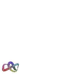
(a) An implosive eddy geometry.

(b) Stable renormalization core.

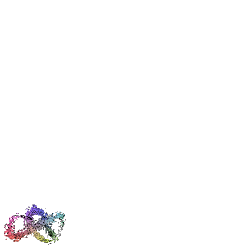
(c) Vanishing renormalization core.

Figure 4: Viscosity implosion.

It follows from equation (88) that if the flow is self-similar and the renormalization core isotropic and $E$ non constant then $V(0)>1$ and for $1<\gamma<V(0)$ the flow is strongly super-diffusive and theorems 4.13, 4.15 and 4.17 are valid (with $\lambda^{-}>0$).
The viscosity implosion of the renormalization core implies that the strong self-averaging property of the flow collapse towards a chaotic coupling between the scales. Let us give a particular example to illustrate what we mean by such bifurcation. The flow is assumed to be self-similar and isotropic and the stream lines of the eddy $E$ over a period $[0,1]^{3}$ are given in the figure 4(a). Since there exists $\delta>0$ such that the drift $\nabla.E$ is null on $[0,1]^{d}\setminus[\delta,1-\delta]^{d}$ we have $\gamma_{c}<\infty$ with the eddy illustrated in figure (4(a)). Now imagine that one puts a drop of dye in such a flow and observe its transport at very large spatial scale. We have illustrated in the figure 4 a metaphorical illustration of what one could see, it would be interesting to run numerical simulations to analyze the behavior of a drop of dye at the transition between a stable and vanishing renormalization core. For $\gamma<\gamma_{c}$ dye is transported by strong super-diffusion, and the density of its colorant in the flow is homogeneous (figure 4(b)). Moreover in the domain $(0,\gamma_{c})$ an increase of the flow rate $\gamma$ in the eddies is compensated by an increase of the diffusive (dissipative) power of the smaller eddies. The picture undergoes a brutal transformation at $\gamma\geq\gamma_{c}$; in this domain an increase of $\gamma$ results in the growth of the advective power of the eddies but their diffusive power remains bounded and can no longer compensate convection. The diffusive power of the smaller scales becomes dominated by the convective power of the eddy at the observation scale (figure 4(c)). The drop dye is then transported by advection and presents high density gradients.

Variational formulae for $\gamma_{c}$.

Assume the flow to be self-similar and isotropic. Thus from equation (71) it is easy to obtain that

$$\gamma_{c}^{-1}=\inf_{(f,H)\in C^{\infty}(\mathbb{T}^{d})\times\mathcal{S}(\mathbb{T}^{d})}\int_{\mathbb{T}^{d}}|\xi-\operatorname{div}H+E\nabla f|^{2}\,dx$$ (91)

from equation (76) it is also easy to obtain that for any unit vector $l$ in $\mathbb{R}^{d}$

$$\gamma_{c}=1+\lim_{\zeta\downarrow 0}\inf_{\xi\perp l,(f,H)\in C^{\infty}(\mathbb{T}^{d})\times\mathcal{S}(\mathbb{T}^{d})}\zeta^{-2}\int_{\mathbb{T}^{d}}|\xi-\operatorname{div}H-E(l-\nabla f)|^{2}\,dx+\int_{\mathbb{T}^{d}}|\nabla f|^{2}\,dx.$$ (92)

Write $G$ the set of $f\in H^{1}(\mathbb{T}^{d})$ such that there exists $\xi,l\in\mathbb{R}^{d}$ and $H$ a skew symmetric matrix with coefficients in $H^{1}(\mathbb{T}^{d})$ with $\xi\perp l$ and

$$\xi-\operatorname{div}H-E(l-\nabla f)=0.$$ (93)

Then if $G=\emptyset$ it is easy to obtain from (92) that $\gamma_{c}=\infty$. If $G\not=\emptyset$ then one has

$$\gamma_{c}=1+\inf_{f\in G}\int_{\mathbb{T}^{d}}|\nabla f|^{2}\,dx.$$ (94)

The equation (93) is degenerate, thus it is not easy to prove a solution for that equation in a general case and actually most of the time it has no solution which means that $\gamma_{c}=\infty$. It would be interesting to obtain non trivial criteria ensuring the existence of a solution for (93). The most trivial example of a stream matrix $E$ such that $\gamma_{c}<\infty$ is the following one. Take $d=2$ and $E$ a skew symmetric matrix with $E_{1,2}=h$ where $h$ over the period $[0,1]^{2}$ is equal to

$$h(x_{1},x_{2})=\sin(2\pi x_{1})\sin(2\pi x_{2})g\Big{(}4\big{(}(x_{1}-0.5)^{2}+(x_{2}-0.5)^{2}\big{)}\Big{)}$$ (95)

where $g$ is any smooth function on [0,1] such that $g=1$ on $[0,1/3]$ and $g=0$ on $[2/3,1]$. Then it is easy to check that $1<\gamma_{c}<\infty$ and estimate it from the variational formulae given above. For instance write $G^{\prime}$ the set of smooth $\mathbb{T}^{d}$ periodic function $f$ such that $\nabla f=e_{2}$ on $\{x\,:\,(x_{1}-0.5)^{2}+(x_{2}-0.5)^{2}\leq 1/6\}$ then it is easy to check that

$$\gamma_{c}\leq 1+\inf_{f\in G^{\prime}}\int_{\mathbb{T}^{d}}|\nabla f|^{2}\,dx.$$ (96)

The renormalization core with a finite number of scales.

The results given above were related to the asymptotic behavior of the renormalization core. When the flow has only a finite number of scales we will give below quantitative estimates controlling the renormalization core.

Theorem 4.31.

The ubiety of the renormalization core is bounded from above by the inverse of its stability. Writing $C=C_{d}K_{0}^{2}(1-1/\gamma_{\min})^{-1}$ we have

$$\lambda^{+}_{n}\leq\kappa+\frac{C}{\lambda^{-}_{n-1}}\quad\text{and}\quad\mu_{n}\leq\frac{\kappa}{\lambda^{-}_{n}}+\frac{C}{(\lambda^{-}_{n})^{2}}$$

Theorem 4.32.

We have

$$\lambda^{-}_{n}\geq\min\Big{(}\lambda_{\min}(\kappa),(\mu_{n})^{-\frac{1}{2}}\frac{V^{-1}(\gamma_{\max})}{\gamma_{\max}}\Big{)}.$$ (97)

Theorem 4.33.

We have for $n\in\mathbb{N}$

$$\lambda^{+}_{n}\leq\max\Big{(}\lambda_{\max}(\kappa),C_{d}K_{0}\mu^{\frac{1}{2}}_{n}(\gamma_{\min}-1)^{-\frac{1}{2}}\Big{)}\big{(}1+W(0)\big{)}.$$ (98)

In particular, observe that if $\gamma_{\max}<\infty$ and $\lambda^{-}=0$ then the stability of the renormalization core should decrease according to the following relation $\ln\lambda^{-}_{n}\sim-0.5\ln\mu_{n}$ and its ubiety should increase like $\ln\lambda^{+}_{n}\sim 0.5\ln\mu_{n}$.

5 Proofs

5.1 Averaging with two scales: proof of theorem 4.1

There are two strategies to prove theorem 4.1; the first one is based on the relative translation method introduced in [Owh01a] and the variational formulations of the effective conductivity; this is the strategy used in [BO02a]. The second one is new and based only on the relative translation method. Although the first strategy in the case considered here would give (the proof is rather long) a sharper estimate of the error term: $(1+\epsilon(R))^{2}$ with $\epsilon(R)=\frac{\|K\|_{\alpha}}{R^{\alpha}\lambda_{\min}(a)}f(d,\frac{\|a+P\|_{\infty}}{\lambda_{\min}(a)})$ instead of (24) we have preferred to write here the second one for its simplicity and the fact that it allows to obtain a lower and an upper bound at once without the need of any variational formulation. Let us now give this new alternative strategy.
By the variational formulation (23) the effective conductivity $\sigma_{{\operatorname{sym}}}(a,S_{R}P+K)$ is continuous in $L^{\infty}(\mathbb{T}^{d})$ norm with respect to the stream matrices $P$ and $K$ and by density it is sufficient to prove the estimate (24) assuming that $P$ and $K$ are smooth and belongs to $\mathcal{S}(\mathbb{T}^{d})$.
First we will prove the following proposition where we have used the notation introduced in section 3 (we write $E:=S_{R}P+K$).

Proposition 5.1.

Let $l\in\mathbb{R}^{d}$, $l\not=0$.

$$\bigg{[}\Big{(}{{}^{t}l}\sigma_{{\operatorname{sym}}}(a,S_{R}P+K)l\Big{)}^{\frac{1}{2}}-\Big{(}{{}^{t}l}\sigma_{{\operatorname{sym}}}\big{(}\sigma_{{\operatorname{sym}}}(a,P),K\big{)}l\Big{)}^{\frac{1}{2}}\bigg{]}^{2}\leq J_{1}+J_{2}+J_{3}+J_{4}$$ (99)

with

$$\begin{split}J_{1}=\int_{(x,y)\in\mathbb{T}^{d}\times[-\frac{1}{2},\frac{1}{2}]^{d}}\nabla F^{a,E}_{l}(x+\frac{y}{R})\big{(}a-E(x+\frac{y}{R})\big{)}\nabla\chi^{a,P}(Rx+y)\nabla F^{\sigma_{{\operatorname{sym}}}(a,P),K}_{l}(x)\,dx\,dy\end{split}$$ (100)

$$\begin{split}J_{2}=-\int_{\mathbb{T}^{d}\times[-\frac{1}{2},\frac{1}{2}]^{d}}\nabla F^{a,E}_{l}(x+\frac{y}{R})\big{(}(a+P(Rx+y))\nabla F^{a,P}(Rx+y)-\sigma_{{\operatorname{sym}}}(a,P)\big{)}\nabla F^{\sigma_{{\operatorname{sym}}}(a,P),K}_{l}(x)\,dx\,dy\end{split}$$ (101)

$$\begin{split}J_{3}=-\int_{\mathbb{T}^{d}\times[-\frac{1}{2},\frac{1}{2}]^{d}}\nabla F^{a,E}_{l}(x+\frac{y}{R})\big{(}K(x+\frac{y}{R})-K(x)\big{)}\nabla F^{a,P}(Rx+y)\nabla F^{\sigma_{{\operatorname{sym}}}(a,P),K}_{l}(x)\,dx\,dy\end{split}$$ (102)

$$\begin{split}J_{4}=\int_{\mathbb{T}^{d}\times[-\frac{1}{2},\frac{1}{2}]^{d}}\nabla F^{a,E}_{l}(x+\frac{y}{R})K(x)\nabla\chi^{a,P}(Rx+y)\nabla F^{\sigma_{{\operatorname{sym}}}(a,P),K}_{l}(x)\,dx\,dy\end{split}$$ (103)

Proof.

Let us write

$$I=\int_{(x,y)\in\mathbb{T}^{d}\times[-\frac{1}{2},\frac{1}{2}]^{d}}\nabla F^{a,E}_{l}(x+\frac{y}{R})a\nabla F^{a,P}(Rx+y)\nabla F^{\sigma_{{\operatorname{sym}}}(a,P),K}_{l}(x)\,dx\,dy.$$ (104)

Using Cauchy-Schwartz inequality and the formula (20) one obtains that

$$I\leq\Big{(}{{}^{t}l}\sigma_{{\operatorname{sym}}}(a,S_{R}P+K)l\Big{)}^{\frac{1}{2}}\Big{(}{{}^{t}l}\sigma_{{\operatorname{sym}}}\big{(}\sigma_{{\operatorname{sym}}}(a,P),K\big{)}l\Big{)}^{\frac{1}{2}}.$$ (105)

Now, writing $E=S_{R}P+K$ observe that

$$I=(I_{1}+I_{2})/2$$ (106)

with

$$\begin{split}I_{1}=\int_{(x,y)\in\mathbb{T}^{d}\times[-\frac{1}{2},\frac{1}{2}]^{d}}\nabla F^{a,E}_{l}(x+\frac{y}{R})\big{(}a+E(x+\frac{y}{R})\big{)}\nabla F^{a,P}(Rx+y)\nabla F^{\sigma_{{\operatorname{sym}}}(a,P),K}_{l}(x)\,dx\,dy\end{split}$$

and

$$\begin{split}I_{2}=\int_{(x,y)\in\mathbb{T}^{d}\times[-\frac{1}{2},\frac{1}{2}]^{d}}\nabla F^{a,E}_{l}(x+\frac{y}{R})\big{(}a-E(x+\frac{y}{R})\big{)}\nabla F^{a,P}(Rx+y)\nabla F^{\sigma_{{\operatorname{sym}}}(a,P),K}_{l}(x)\,dx\,dy.\end{split}$$

Using

$$\begin{split}\int_{(x,y)\in\mathbb{T}^{d}\times[-\frac{1}{2},\frac{1}{2}]^{d}}\nabla F^{a,E}_{l}(x+\frac{y}{R})\big{(}a-E(x+\frac{y}{R})\big{)}l={{}^{t}l}\sigma_{{\operatorname{sym}}}(a,S_{R}P+K)l\end{split}$$

and the fact that $\nabla F^{a,E}_{l}(x+\frac{y}{R})\big{(}a-E(x+\frac{y}{R})\big{)}$ is a divergence free vector field one obtains that

$$\begin{split}I_{2}=&{{}^{t}l}\sigma_{{\operatorname{sym}}}(a,S_{R}P+K)l-J_{1}\end{split}$$

with $J_{1}$ given by (100). Moreover

$$\begin{split}I_{1}=G_{0}-J_{2}-J_{3}-J_{4}\end{split}$$ (107)

with

$$\begin{split}G_{0}=&\int_{(x,y)\in\mathbb{T}^{d}\times[-\frac{1}{2},\frac{1}{2}]^{d}}\nabla F^{a,E}_{l}(x+\frac{y}{R})\big{(}\sigma_{{\operatorname{sym}}}(a,P)+K(x)\big{)}\nabla F^{\sigma_{{\operatorname{sym}}}(a,P),K}_{l}(x)\,dx\,dy\\ =&{{}^{t}l}\sigma_{{\operatorname{sym}}}\big{(}\sigma_{{\operatorname{sym}}}(a,P),K\big{)}l\end{split}$$ (108)

where we have used in the last equality the fact that $\big{(}\sigma_{{\operatorname{sym}}}(a,P)+K(x)\big{)}\nabla F^{\sigma_{{\operatorname{sym}}}(a,P),K}_{l}(x)$ is divergence free. And $J_{2}$, $J_{3}$, $J_{4}$ are given by (101), (102) and (103). Thus combining (105) and (106) we have obtained (99), which proves the proposition. ∎

Now we will show that $J_{1}$, $J_{2}$, $J_{3}$ and $J_{4}$ act as error terms in the homogenization process.
Using $\operatorname{div}\big{(}(a+E)\nabla F^{a,E}_{l}\big{)}=0$ and observing that, $\nabla\chi^{a,P}(Rx+y)=\nabla_{y}\chi^{a,P}(Rx+y)$ and integrating by parts in $y$ one obtains (writing $\partial^{i}([-\frac{1}{2},\frac{1}{2}]^{d})=\{x\in[-\frac{1}{2},\frac{1}{2}]^{d}\,:\,x_{i}=-\frac{1}{2}\}$)

$$J_{1}=G_{1}+G_{2}$$ (109)

with (writing $(e_{i})_{1\leq i\leq d}$ the orthonormal basis of $\mathbb{R}^{d}$ compatible with the axis of periodicity of $\mathbb{T}^{d}$)

$$\begin{split}G_{1}=&\sum_{i=1}^{d}\int_{(x,y^{i})\in\mathbb{T}^{d}\times\partial^{i}([-\frac{1}{2},\frac{1}{2}]^{d})}{{}^{t}\big{(}\nabla F^{a,E}_{l}(x+(y^{i}+e_{i})/R)-\nabla F^{a,E}_{l}(x+y^{i}/R)\big{)}}(a-P(Rx+y^{i})).e_{i}\\ &\chi^{a,P}(Rx+y^{i})\nabla F^{\sigma_{{\operatorname{sym}}}(a,P),K}_{l}(x)\,dx\,dy^{i}\end{split}$$ (110)

$$\begin{split}G_{2}=-&\sum_{i=1}^{d}\int_{(x,y^{i})\in\mathbb{T}^{d}\times\partial^{i}([-\frac{1}{2},\frac{1}{2}]^{d})}\big{(}{{}^{t}\nabla F^{a,E}_{l}(x+(y^{i}+e_{i})/R)}K(x+(y^{i}+e_{i})/R)\\ &-{{}^{t}\nabla F^{a,E}_{l}(x+y^{i}/R)}K(x+y^{i}/R)\big{)}.e_{i}\chi^{a,P}(Rx+y^{i})\nabla F^{\sigma_{{\operatorname{sym}}}(a,P),K}_{l}(x)\,dx\,dy^{i}.\end{split}$$ (111)

Now we will need the following lemma which says that the solution of the two-scale cell problem keeps in its structure a signature of the fast period.

Lemma 5.2.

For $i\in\{1,\ldots d\}$ one has

$$\begin{split}\int_{x\in\mathbb{T}^{d}}|\nabla F^{a,E}_{l}(x+e_{i}/R)-\nabla F^{a,E}_{l}(x)|_{a}^{2}\leq|l|^{2}_{\sigma(a,E)}C_{d}(\frac{\|K\|_{\alpha}}{R^{\alpha}\lambda_{\min}(a)})^{2}.\end{split}$$ (112)

Proof.

Observe that

$$\nabla.(a+E(x))\nabla\big{(}F^{a,E}_{l}(x+e_{i}/R)-F^{a,E}_{l}(x)\big{)}=\nabla.\Big{(}\big{(}K(x)-K(x+e_{i}/R)\big{)}\nabla F^{a,E}_{l}(x+e_{i}/R)\Big{)}.$$ (113)

It follows that

$$\begin{split}\int_{x\in\mathbb{T}^{d}}|\nabla F^{a,E}_{l}(x+e_{i}/R)-\nabla F^{a,E}_{l}(x)|_{a}^{2}=&\int_{x\in\mathbb{T}^{d}}\big{(}\nabla F^{a,E}_{l}(x+e_{i}/R)-\nabla F^{a,E}_{l}(x)\big{)}\\ &\big{(}K(x)-K(x+e_{i}/R)\big{)}\nabla F^{a,E}_{l}(x+e_{i}/R)\end{split}$$ (114)

thus using Cauchy-Schwartz inequality one obtains

$$\begin{split}\int_{x\in\mathbb{T}^{d}}|\nabla F^{a,E}_{l}(x+e_{i}/R)-\nabla F^{a,E}_{l}(x)|_{a}^{2}\leq\int_{x\in\mathbb{T}^{d}}\Big{|}(K(x)-K(x+e_{i}/R))\nabla F^{a,E}(x+e_{i}/R)\Big{|}^{2}_{a^{-1}}\end{split}$$ (115)

and the equation 112 follows easily. ∎

It follows from lemma 5.2 equation 110 and Cauchy-Schwartz inequality that

$$\begin{split}G_{1}\leq C_{d}\frac{\|K\|_{\alpha}}{R^{\alpha}\lambda_{\min}(a)}\|\chi^{a,P}\|_{\infty}\frac{\|a-P\|_{\infty}}{\lambda_{\min}(a)}\Big{(}{{}^{t}l}\sigma_{{\operatorname{sym}}}(a,S_{R}P+K)l\Big{)}^{\frac{1}{2}}\Big{(}{{}^{t}l}\sigma_{{\operatorname{sym}}}\big{(}\sigma_{{\operatorname{sym}}}(a,P),K\big{)}l\Big{)}^{\frac{1}{2}}.\end{split}$$ (116)

Now we will use the following lemma which is a consequence of Stampacchia estimates [Sta66], [Sta65] for elliptic operators with discontinuous coefficients (see [Owh01a], appendix B, theorem B.1.1) (we remind that $\chi^{a,P}$ is uniquely defined by the cell problem and $\int_{\mathbb{T}^{d}}\chi^{a,P}(x)\,dx=0$)

Lemma 5.3.

$$\|\chi^{a,P}\|_{\infty}\leq C_{d}\big{(}\frac{\|a+P\|_{\infty}}{\lambda_{\min}(a)}\big{)}^{3d+2}$$ (117)

Thus one obtains from (117) and (116) that

$$\begin{split}G_{1}\leq C_{d}\frac{\|K\|_{\alpha}}{R^{\alpha}\lambda_{\min}(a)}\big{(}\frac{\|a+P\|_{\infty}}{\lambda_{\min}(a)}\big{)}^{3d+3}\Big{(}{{}^{t}l}\sigma_{{\operatorname{sym}}}(a,S_{R}P+K)l\Big{)}^{\frac{1}{2}}\Big{(}{{}^{t}l}\sigma_{{\operatorname{sym}}}\big{(}\sigma_{{\operatorname{sym}}}(a,P),K\big{)}l\Big{)}^{\frac{1}{2}}\end{split}$$ (118)

similarly, observing that $\operatorname{div}_{y}\big{(}K(x)\nabla F^{a,E}_{l}(x+\frac{y}{R})\big{)}=0$ and integrating by part in $y$ in the equation (103) one obtains

$$\begin{split}J_{4}=&\sum_{i=1}^{d}\int_{(x,y^{i})\in\mathbb{T}^{d}\times\partial^{i}([-\frac{1}{2},\frac{1}{2}]^{d})}\big{(}{{}^{t}\nabla F^{a,E}_{l}(x+(y^{i}+e_{i})/R)}-{{}^{t}\nabla F^{a,E}_{l}(x+y^{i}/R)}\big{)}K(x).e_{i}\\ &\chi^{a,P}(Rx+y^{i})\nabla F^{\sigma_{{\operatorname{sym}}}(a,P),K}_{l}(x)\,dx\,dy^{i}.\end{split}$$ (119)

Adding equation (111) to equation (119) we obtain

$$\begin{split}J_{4}+G_{2}=&\sum_{i=1}^{d}\int_{(x,y^{i})\in\mathbb{T}^{d}\times\partial^{i}([-\frac{1}{2},\frac{1}{2}]^{d})}{{}^{t}\nabla F^{a,E}_{l}(x+(y^{i}+e_{i})/R)}\big{(}K(x)-K(x+(y^{i}+e_{i})/R)\big{)}.e_{i}\\ &\chi^{a,P}(Rx+y^{i})\nabla F^{\sigma_{{\operatorname{sym}}}(a,P),K}_{l}(x)\,dx\,dy^{i}\\ &+\sum_{i=1}^{d}\int_{(x,y^{i})\in\mathbb{T}^{d}\times\partial^{i}([-\frac{1}{2},\frac{1}{2}]^{d})}{{}^{t}\nabla F^{a,E}_{l}(x+y^{i}/R)}\big{(}K(x+y^{i}/R)-K(x)\big{)}.e_{i}\\ &\chi^{a,P}(Rx+y^{i})\nabla F^{\sigma_{{\operatorname{sym}}}(a,P),K}_{l}(x)\,dx\,dy^{i}\end{split}$$ (120)

and by Cauchy Schwartz inequality and lemma 117 one obtains that

$$\begin{split}J_{4}+G_{2}\leq C_{d}\frac{\|K\|_{\alpha}}{R^{\alpha}\lambda_{\min}(a)}\big{(}\frac{\|a+P\|_{\infty}}{\lambda_{\min}(a)}\big{)}^{3d+3}\Big{(}{{}^{t}l}\sigma_{{\operatorname{sym}}}(a,S_{R}P+K)l\Big{)}^{\frac{1}{2}}\Big{(}{{}^{t}l}\sigma_{{\operatorname{sym}}}\big{(}\sigma_{{\operatorname{sym}}}(a,P),K\big{)}l\Big{)}^{\frac{1}{2}}.\end{split}$$ (121)

Moreover from equation (102) and Cauchy Schwartz inequality one easily obtains

$$\begin{split}J_{3}\leq C_{d}\frac{\|K\|_{\alpha}}{R^{\alpha}\lambda_{\min}(a)}\Big{(}{{}^{t}l}\sigma_{{\operatorname{sym}}}(a,S_{R}P+K)l\Big{)}^{\frac{1}{2}}\Big{(}{{}^{t}l}\sigma_{{\operatorname{sym}}}\big{(}\sigma_{{\operatorname{sym}}}(a,P),K\big{)}l\Big{)}^{\frac{1}{2}}.\end{split}$$ (122)

Now we will need the following lemma

Lemma 5.4.

If $V\in(C^{\infty}(\mathbb{T}^{d}))^{d}$ is such that $\operatorname{div}V=0$ and $\int_{\mathbb{T}^{d}}V(x)dx=0$ then for $p>d$, there exists a skew symmetric $\mathbb{T}^{d}$-periodic matrix $M$ such that $\|M\|_{\infty}\leq C_{d,p}\|V\|_{L^{p}(\mathbb{T}^{d})}$ and $V=\nabla.M$.

Proof.

From the proof of lemma 4.7 of [BO02a] one obtains that there exists a $\mathbb{T}^{d}$-periodic smooth skew-symmetric matrix $M$ such that

$$V_{i}=\sum_{j=1}^{d}M_{ij}$$ (123)

and $M$ is given by

$$M_{ij}=B^{j}_{i}-B^{i}_{j}$$ (124)

where $B^{i}_{j}$ are the smooth $\mathbb{T}^{d}$ periodic solutions of

$$\Delta B^{i}_{j}=\partial_{i}V_{j}$$ (125)

with $0$ mean Lebesgue measure. Using the theorem 5.4 of [Sta66] one obtains that for $p>d$

$$\|B^{i}_{j}\|_{\infty}\leq C_{d,p}\|V_{j}\|_{L^{p}(\mathbb{T}^{d})}$$ (126)

which proves the lemma. ∎

Let us now prove the following lemma.

Lemma 5.5.

$$\Big{(}\big{(}a+P(Rx+y)\big{)}\nabla F^{a,P}(Rx+y)-\sigma(P)\Big{)}_{kj}=\sum_{i=1}^{d}\partial_{i}M^{P}_{kij}(Rx+y)$$ (127)

where $M^{P}$ is a $\mathbb{T}^{d}$ periodic $d\times d\times d$ tensor such that $M^{P}_{ikj}=-M^{P}_{kij}$ and

$$\|M^{P}\|_{\infty}\leq C_{d,\|a+P\|_{\infty}/\lambda_{\min}(a)}\|a+P\|_{\infty}.$$ (128)

Proof.

From lemma 5.4 one obtains that for $p>d$,

$$\|M^{P}\|_{\infty}\leq C_{d,p}\|\big{(}a+P(.))\nabla F^{a,P}(.)-\sigma(P)\big{)}\|_{L^{p}(\mathbb{T}^{d})}.$$ (129)

Using Meyers argument [Mey63] one obtains that there exists $p(\|a+E\|_{\infty}/\lambda_{\min}(a))>d$ such that

$$\|\nabla\chi^{a,P}(.)\|_{L^{p}(\mathbb{T}^{d})}\leq C_{d,\|a+P\|_{\infty}/\lambda_{\min}(a)}.$$ (130)

Which implies equation (128). ∎

Using equation (127) and integrating by part in $y$ in (101) one obtains

$$\begin{split}J_{2}=&-\sum_{i,j,k=1}^{d}\int_{(x,y^{i})\in\mathbb{T}^{d}\times\partial^{i}([-\frac{1}{2},\frac{1}{2}]^{d})}\big{(}{{}^{t}\nabla F^{a,E}_{l}(x+(y^{i}+e_{i})/R)}-{{}^{t}\nabla F^{a,E}_{l}(x+y^{i}/R)}\big{)}.e_{k}\\ &M^{P}_{kij}(Rx+y^{i})e_{j}.\nabla F^{\sigma_{{\operatorname{sym}}}(a,P),K}_{l}(x)\,dx\,dy^{i}.\end{split}$$ (131)

Combining this with (128) and (112) one obtains from Cauchy-Schwartz inequality that

$$\begin{split}J_{2}\leq C_{d,\|a+P\|_{\infty}/\lambda_{\min}(a)}\frac{\|K\|_{\alpha}}{R^{\alpha}\lambda_{\min}(a)}\Big{(}{{}^{t}l}\sigma_{{\operatorname{sym}}}(a,S_{R}P+K)l\Big{)}^{\frac{1}{2}}\Big{(}{{}^{t}l}\sigma_{{\operatorname{sym}}}\big{(}\sigma_{{\operatorname{sym}}}(a,P),K\big{)}l\Big{)}^{\frac{1}{2}}.\end{split}$$ (132)

In conclusion we have obtained from equations (99), (109), (118), (121), (122) and (132) that

$$\begin{split}\bigg{[}\Big{(}{{}^{t}l}\sigma_{{\operatorname{sym}}}(a,S_{R}P+K)l\Big{)}^{\frac{1}{2}}-&\Big{(}{{}^{t}l}\sigma_{{\operatorname{sym}}}\big{(}\sigma_{{\operatorname{sym}}}(a,P),K\big{)}l\Big{)}^{\frac{1}{2}}\bigg{]}^{2}\leq C_{d,\|a+P\|_{\infty}/\lambda_{\min}(a)}\frac{\|K\|_{\alpha}}{R^{\alpha}\lambda_{\min}(a)}\\ &\Big{(}{{}^{t}l}\sigma_{{\operatorname{sym}}}(a,S_{R}P+K)l\Big{)}^{\frac{1}{2}}\Big{(}{{}^{t}l}\sigma_{{\operatorname{sym}}}\big{(}\sigma_{{\operatorname{sym}}}(a,P),K\big{)}l\Big{)}^{\frac{1}{2}}.\end{split}$$ (133)

Now we will use the following lemma whose proof is trivial

Lemma 5.6.

If $(X-Y)^{2}\leq\delta XY$ then $X/Y\leq(1+8\sqrt{\delta})^{2}$

And the estimate (24) is a simple consequence of (133) and lemma 5.6 which proves the theorem.

5.2 Averaging with $n$ scales: Proof of theorem 4.4

The proof of theorem 4.4 is based on theorem 4.1 and a reverse induction. It is important to note that contrary to reiterated homogenization, here the larger scales are homogenized first, this reversion in the inductive process is essential to obtain sharp estimates. Observe that by the variational formula 17 one has for $\gamma>0$, $B\in\mathcal{M}_{d,{\operatorname{sym}}}$ and $K\in\mathcal{S}_{L^{\infty}}(\mathbb{T}^{d})$,

$$\sigma_{sym}(B,\gamma K)=\gamma\sigma_{sym}(\frac{B}{\gamma},K).$$ (134)

From this we deduce that for $p\in\{0,\ldots,n-1\}$

$$\sigma_{sym}(\sigma_{sym}(B,E^{p}),\frac{1}{\gamma_{p}}\Gamma^{p+1,n})=\frac{\gamma_{p+1}}{\gamma_{p}}\sigma_{sym}(\frac{\gamma_{p}}{\gamma_{p+1}}\sigma_{sym}(B,E^{p}),\frac{1}{\gamma_{p+1}}\Gamma^{p+1,n}).$$ (135)

Combining this with the theorem 4.1 one obtains that for $p\in\{0,\ldots,n-1\}$

$$\begin{split}\sigma_{sym}(B,\frac{1}{\gamma_{p}}\Gamma^{p,n})\leq\frac{\gamma_{p+1}}{\gamma_{p}}\sigma_{sym}(\frac{\gamma_{p}}{\gamma_{p+1}}\sigma_{sym}(B,E^{p}),\frac{1}{\gamma_{p+1}}\Gamma^{p+1,n})(1+\epsilon_{p+1}(B))^{4}\end{split}$$ (136)

$$\begin{split}\sigma_{sym}(B,\frac{1}{\gamma_{p}}\Gamma^{p,n})\geq\frac{\gamma_{p+1}}{\gamma_{p}}\sigma_{sym}(\frac{\gamma_{p}}{\gamma_{p+1}}\sigma_{sym}(B,E^{p}),\frac{1}{\gamma_{p+1}}\Gamma^{p+1,n})(1+\epsilon_{p+1}(B))^{-4}\end{split}$$ (137)

with

$$\begin{split}\epsilon_{p}(B)=&\Big{(}\frac{\gamma_{p}K_{\alpha}}{\gamma_{p-1}r_{p}^{\alpha}\lambda_{\min}(B)(1-\gamma_{\max}/\rho_{\min}^{\alpha})}\Big{)}^{\frac{1}{2}}f\big{(}(d,(\lambda_{\max}(B)+K_{0})/\lambda_{\min}(B)\big{)}).\end{split}$$ (138)

Then one obtains by a simple induction that

$$\begin{split}\gamma_{n+1}A^{n+1}\prod_{p=0}^{n-1}(1+\epsilon_{p+1}(A^{p}))^{-4}\leq\sigma_{sym}(a,\Gamma^{0,n})\leq\gamma_{n+1}A^{n+1}\prod_{p=0}^{n-1}(1+\epsilon_{p+1}(A^{p}))^{4}.\end{split}$$ (139)

Where $A^{k}$, is the renormalization coreization sequence given in definition 4.3 which proves theorem 4.4.

5.3 Diagnosis of renormalization core’s pathologies: proofs

Let $a\in\mathcal{M}_{d,{\operatorname{sym}}}$ and $E\in\mathcal{S}_{L^{\infty}}(\mathbb{T}^{d})$, it is well known ([AM91]) and a simple consequence of (17) and (23) that

$$a\leq\sigma_{{\operatorname{sym}}}(a,E)\leq a+\int_{\mathbb{T}^{d}}{{}^{t}E(x)a^{-1}E(x)}\,dx.$$ (140)

Then the following proposition follows from (33), (140) and a simple induction on the number of scales.

Proposition 5.7.

For all $n\in\mathbb{N}$

$$\gamma_{n}^{-1}I_{d}\leq A^{n}\leq(\kappa/\gamma_{n})I_{d}+\sum_{p=0}^{n-1}(\gamma_{p}/\gamma_{n})\int_{T^{d}_{1}}{{}^{t}E^{p}(x)(A^{p})^{-1}E^{p}(x)}\,dx.$$ (141)

Theorems 4.20 and 4.31 are straightforward consequences of proposition 5.7. We will need the following proposition giving isotropic estimates on anisotropic viscosities.

Proposition 5.8.

For $a\in\mathcal{M}_{d,{\operatorname{sym}}}$ and $E\in\mathcal{S}_{L^{\infty}}(\mathbb{T}^{d})$, one has for all $l\in(\mathbb{R}^{d})^{*}$

$$\begin{split}\big{(}\frac{\lambda_{\max}(a)}{\lambda_{\min}(a)}\big{)}^{-\frac{1}{2}}\leq\frac{{}^{t}l\sigma_{{\operatorname{sym}}}(a,E)l}{{}^{t}l\sigma_{{\operatorname{sym}}}\Big{(}\big{(}\lambda_{\max}(a)\lambda_{\min}(a)\big{)}^{\frac{1}{2}}I_{d},E\Big{)}l}\leq\big{(}\frac{\lambda_{\max}(a)}{\lambda_{\min}(a)}\big{)}^{\frac{1}{2}}.\end{split}$$ (142)

Proof.

By the variational formula 17 one has for $\xi\in\mathbb{R}^{d}$

$$\begin{split}|\xi|_{\sigma_{{\operatorname{sym}}}^{-1}(a,E)}^{2}=&\inf_{(f,H)\in C^{\infty}(\mathbb{T}^{d})\times\mathcal{S}(\mathbb{T}^{d})}\int_{\mathbb{T}^{d}}|\xi-\nabla.H+E\nabla f|_{a^{-1}}^{2}\,dx+\int_{\mathbb{T}^{d}}|\nabla f(x)|_{a}^{2}\,dx\\ \leq&\big{(}\lambda_{\max}(a)/\lambda_{\min}(a)\big{)}^{\frac{1}{2}}\inf_{(f,H)\in C^{\infty}(\mathbb{T}^{d})\times\mathcal{S}(\mathbb{T}^{d})}\big{(}\lambda_{\max}(a)\lambda_{\min}(a)\big{)}^{-\frac{1}{2}}\int_{\mathbb{T}^{d}}|\xi-\nabla.H+E\nabla f|^{2}\,dx\\ &+\big{(}\lambda_{\max}(a)\lambda_{\min}(a)\big{)}^{\frac{1}{2}}\int_{\mathbb{T}^{d}}|\nabla f(x)|^{2}\,dx.\end{split}$$ (143)

It follows that

$$\begin{split}\sigma_{{\operatorname{sym}}}(a,E)\geq\big{(}\lambda_{\max}(a)/\lambda_{\min}(a)\big{)}^{-\frac{1}{2}}\sigma_{{\operatorname{sym}}}\Big{(}\big{(}\lambda_{\max}(a)\lambda_{\min}(a)\big{)}^{\frac{1}{2}}I_{d},E\Big{)}.\end{split}$$ (144)

Similarly from the variational formula 23 one obtains that for $l\in\mathbb{R}^{d}$

$$\begin{split}|l|_{\sigma_{{\operatorname{sym}}}}^{2}=&\inf_{\xi\perp l,(f,H)\in C^{\infty}(\mathbb{T}^{d})\times\mathcal{S}(\mathbb{T}^{d})}\int_{\mathbb{T}^{d}}|\xi-\nabla.H-E(l-\nabla f)|^{2}_{a^{-1}}\,dx+\int_{\mathbb{T}^{d}}|l-\nabla f|^{2}_{a}\,dx\\ \leq&\big{(}\lambda_{\max}(a)/\lambda_{\min}(a)\big{)}^{\frac{1}{2}}\inf_{\xi\perp l,(f,H)\in C^{\infty}(\mathbb{T}^{d})\times\mathcal{S}(\mathbb{T}^{d})}\\ &\big{(}\lambda_{\max}(a)\lambda_{\min}(a)\big{)}^{-\frac{1}{2}}\int_{\mathbb{T}^{d}}|\xi-\nabla.H-E(l-\nabla f)|^{2}\,dx+\big{(}\lambda_{\max}(a)\lambda_{\min}(a)\big{)}^{\frac{1}{2}}\int_{\mathbb{T}^{d}}|l-\nabla f|^{2}_{a}\,dx.\end{split}$$ (145)

Which leads us to

$$\begin{split}\sigma_{{\operatorname{sym}}}(a,E)\leq\big{(}\lambda_{\max}(a)/\lambda_{\min}(a)\big{)}^{\frac{1}{2}}\sigma_{{\operatorname{sym}}}\Big{(}\big{(}\lambda_{\max}(a)\lambda_{\min}(a)\big{)}^{\frac{1}{2}}I_{d},E\Big{)}.\end{split}$$ (146)

∎

A direct consequence of proposition 5.8 is the following corollary which controls the minimal and maximal enhancement of the conductivity in the flow associated to the stream matrix $E$ by the geometric mean $\big{(}\lambda_{\max}(a)\lambda_{\min}(a)\big{)}^{\frac{1}{2}}$ of the maximal and minimal eigenvalues of $a$.

Corollary 5.9.

$$\begin{split}\frac{\lambda_{\min}\big{(}\sigma_{{\operatorname{sym}}}(a,E)\big{)}}{\lambda_{\min}(a)}\geq\frac{\lambda_{\min}\bigg{(}\sigma_{{\operatorname{sym}}}\Big{(}\big{(}\lambda_{\max}(a)\lambda_{\min}(a)\big{)}^{\frac{1}{2}}I_{d},E\Big{)}\bigg{)}}{\big{(}\lambda_{\max}(a)\lambda_{\min}(a)\big{)}^{\frac{1}{2}}}\end{split}$$ (147)

$$\begin{split}\frac{\lambda_{\max}\big{(}\sigma_{{\operatorname{sym}}}(a,E)\big{)}}{\lambda_{\max}(a)}\leq\frac{\lambda_{\max}\bigg{(}\sigma_{{\operatorname{sym}}}\Big{(}\big{(}\lambda_{\max}(a)\lambda_{\min}(a)\big{)}^{\frac{1}{2}}I_{d},E\Big{)}\bigg{)}}{\big{(}\lambda_{\max}(a)\lambda_{\min}(a)\big{)}^{\frac{1}{2}}}.\end{split}$$ (148)

It is then a simple consequence of corollary 5.9 that

Proposition 5.10.

$$\frac{\lambda_{\min}(\sigma_{{\operatorname{sym}}}(a,E))}{\lambda_{\min}(a)}\geq V\Big{(}\big{(}\lambda_{\min}(a)\lambda_{\max}(a)\big{)}^{\frac{1}{2}},E\Big{)}$$ (149)

and

$$\frac{\lambda_{\max}(\sigma_{{\operatorname{sym}}}(a,E))}{\lambda_{\max}(a)}\leq W\Big{(}\big{(}\lambda_{\min}(a)\lambda_{\max}(a)\big{)}^{\frac{1}{2}},E\Big{)}.$$ (150)

From proposition 5.10 one obtains that for $n\in\mathbb{N}$,

$$\frac{\lambda_{\min}(A^{n+1})}{\lambda_{\min}(A^{n})}\geq\frac{\gamma_{n}}{\gamma_{n+1}}V\Big{(}\big{(}\lambda_{\min}(A^{n})\lambda_{\max}(A^{n})\big{)}^{\frac{1}{2}},E^{n}\Big{)}.$$ (151)

It follows from the equation (151) and the monotony of $V$ that

$$\frac{\lambda_{\min}(A^{n+1})}{\lambda_{\min}(A^{n})}\geq\frac{1}{\gamma_{max}}V\big{(}\lambda_{\min}(A^{n})(\frac{\lambda_{\max}(A^{n})}{\lambda_{\min}(A^{n})})^{\frac{1}{2}}\big{)}$$ (152)

it follows from (152) that $\lambda_{\min}(A^{n})$ is increasing if it belongs to $\Big{(}0,(\frac{\lambda_{\max}(A^{n})}{\lambda_{\min}(A^{n})})^{-\frac{1}{2}}V^{-1}(\gamma_{\max})\Big{)}$; which implies equation (83) of theorem 4.20 and equation (97) of theorem 4.32.
Now, observe that from the variational formulation (76) one obtains that

$$W(\zeta,E)\leq 1+\zeta^{-2}\lambda_{\max}\Big{(}\int_{\mathbb{T}^{d}}{{}^{t}E(x)E(x)}dx\Big{)}.$$ (153)

It follows from the proposition 5.10 that

$$\frac{\lambda_{\max}(\sigma_{{\operatorname{sym}}}(a,E))}{\lambda_{\max}(a)}\leq 1+C_{d}K_{0}^{2}\big{(}\lambda_{\min}(a)\lambda_{\max}(a)\big{)}^{-1}.$$ (154)

Thus one obtains for all $n\in\mathbb{N}$

$$\frac{\lambda_{\max}(A^{n+1})}{\lambda_{\max}(A^{n})}\leq\gamma_{\min}^{-1}\Big{(}1+C_{d}K_{0}^{2}\frac{\lambda_{\max}(A^{n})}{\lambda_{\min}(A^{n})}\big{(}\lambda_{\max}(A^{n})\big{)}^{-2}\Big{)}.$$ (155)

It follows from (155) that $\lambda_{\max}(A^{n})$ is decreasing if it belongs to $\Big{(}\big{(}C_{d}K_{0}^{2}\frac{\lambda_{\max}(A^{n})}{\lambda_{\min}(A^{n})}(\gamma_{\min}-1)^{-1}\big{)}^{\frac{1}{2}},\infty\Big{)}$ ; which implies the equation (84) of theorem 4.20 and equation (98) of theorem 4.33.
Now observe that by proposition 5.10 one has

$$\frac{\lambda_{\max}(A^{n+1})}{\lambda_{\max}(A^{n})}\leq\frac{1}{\gamma_{min}}W\big{(}\lambda_{\min}(A^{n})(\frac{\lambda_{\max}(A^{n})}{\lambda_{\min}(A^{n})})^{\frac{1}{2}}\big{)}$$ (156)

which proves theorem 4.27 since $W$ is decreasing.
Now if the flow is self-similar and isotropic, theorem 4.30 is a simple consequence of the following recursive relation:

$$\frac{\lambda(A^{n+1})}{\lambda(A^{n})}=\frac{1}{\gamma}V\big{(}\lambda(A^{n})\big{)}.$$ (157)

5.4 Super diffusion: proofs

5.4.1 A variational formula for the exit times

Let $\Omega$ be a smooth subset of $\mathbb{R}^{d}$, we write for $a\in\mathcal{M}_{d,{\operatorname{sym}}}$ and $E$ a skew symmetric matrix with coefficients in $L^{\infty}(\bar{\Omega})$,

$$\psi^{a,E}=\mathbb{E}_{x}[\tau^{a,E}(\Omega)]$$ (158)

the expectation of the exit time from $\Omega$ of the diffusion associated to the generator $\nabla.(a+E)\nabla$ started from $x$. Observe that $\psi^{a,E}$ can be defined as the weak solution of the following equation with null Dirichlet boundary condition on $\partial\Omega$,

$$\nabla.\Big{(}\big{(}a+E(x)\big{)}\nabla\psi^{a,E}(x)\Big{)}=-1.$$ (159)

We will need the following variational formulation for the mean exit times.

Theorem 5.11.

$$\int_{\Omega}\mathbb{E}_{x}[\tau^{a,E}(\Omega)]\,dx=\sup_{f\in C^{\infty}_{0}(\Omega),H\in\mathcal{S}(\bar{\Omega})}\Big{[}2\int_{\Omega}f(x)dx-\int_{\Omega}|\nabla f|_{a}^{2}dx-\int_{\Omega}|\nabla.H+E\nabla f|_{a^{-1}}^{2}dx\Big{]}$$ (160)

Where the minimization (160) is done over smooth functions $f$ on $\Omega$, null on $\partial\Omega$ and smooth skew symmetric matrices $H$ on $\bar{\Omega}$. From theorem 5.11 we deduce the following corollary

Corollary 5.12.

$$\int_{\Omega}\mathbb{E}_{x}[\tau^{a+\lambda I_{d},0}(\Omega)]\,dx\leq\int_{\Omega}\mathbb{E}_{x}[\tau^{a,E}(\Omega)]\,dx\leq\int_{\Omega}\mathbb{E}_{x}[\tau^{a,0}(\Omega)]\,dx$$ (161)

with

$$\lambda:=\sup_{x\in\Omega}\lambda_{\max}\big{(}{{}^{t}E(x)a^{-1}E(x)}\big{)}$$ (162)

Let us now prove theorem 5.11. By density we can first assume $E$ to be smooth. Our purpose is to show that

$$\int_{\Omega}\mathbb{E}_{x}[\tau^{a,E}(\Omega)]\,dx=-2\inf_{f\in C^{\infty}_{0}(\Omega),H\in\mathcal{S}(\bar{\Omega})}\Big{[}\frac{1}{2}\int_{\Omega}|\nabla.H+(a-E)\nabla f|_{a^{-1}}^{2}dx-\int_{\Omega}f(x)dx\Big{]}.$$ (163)

By considering variations around the minimum one obtains that

$$\nabla.H_{0}+(a-E)\nabla f_{0}=a\nabla\psi(x)$$ (164)

with $\psi=0$ on $\partial\Omega$ and

$$\nabla.(a+E)\nabla\psi(x)=-1.$$ (165)

From which one obtains that $\psi(x)=\mathbb{E}_{x}[\tau^{E}(\Omega)]$ and $f_{0}(x)=\big{(}\mathbb{E}_{x}[\tau^{E}(\Omega)]+\mathbb{E}_{x}[\tau^{-E}(\Omega)]\big{)}/2$. Thus at the minimum

$$\begin{split}-\inf_{H,f}\Big{[}\frac{1}{2}\int_{\Omega}|\nabla.H+(a-E)\nabla f|_{a^{-1}}^{2}dx-\int_{\Omega}f(x)dx\Big{]}&=-\Big{[}\frac{1}{2}\int_{\Omega}{{}^{t}\nabla f_{0}}(a+E)\nabla\psi dx-\int_{\Omega}f_{0}(x)dx\Big{]}\\ &=-1/2\int_{\Omega}f_{0}(x)dx\end{split}$$ (166)

since

$$\begin{split}\int_{\Omega}{{}^{t}\nabla f_{0}}(a+E)\nabla\psi(x)dx=\int_{\Omega}|a\nabla\psi(x)|^{2}_{a^{-1}}dx\end{split}$$ (167)

but also

$$\begin{split}\int_{\Omega}|a\nabla\psi(x)|^{2}_{a^{-1}}dx=\int_{\Omega}{{}^{t}\nabla\psi(x)}(a+E)\nabla\psi(x)dx=\int_{\Omega}\psi(x)dx\end{split}$$ (168)

which leads to the result, which can be written as (160).

5.4.2 Averaging with two scales the exit times

We will use the notation of subsection 5.4.1 and assume that

$$E=P(Rx)+K(x).$$ (169)

Where $x\in\Omega$, $R\in[2,\infty)$, $P$ belongs to $\mathcal{S}_{L^{\infty}}(\mathbb{T}^{d})$ and $K$ is a Lipschitz-continuous skew symmetric matrix on $\mathbb{R}^{d}$ ($\alpha=1$). Our purpose is to obtain sharp quantitative estimates on the mean exit time.

$$\int_{\Omega}\psi^{a,E}(x)\,dx.$$ (170)

It follows from theorem 5.11 that the mean exit time (170) is continuous in $L^{\infty}$ norm with respect to $E$, thus we can by density assume $E,P$ and $K$ to be smooth and $\psi^{a,E}$ shall be a strong solution of (159).
To estimate (170) we will need to introduce a relative translation with respect to the fast scale associated to the medium $E$, i.e. we introduce for $x,y\in\Omega\times[0,1]^{d}$, $E(x,y)$ as

$$E(x,y):=P(Rx+y)+K(x).$$ (171)

We will write for $y\in[0,1]^{d}$, $\psi^{a,E}(x,y)$ the strong solution of the following equation with null Dirichlet boundary condition on $\partial\Omega$.

$$\nabla_{x}\Big{(}\big{(}a+E(x,y)\big{)}\nabla_{x}\psi^{a,E}(x,y)\Big{)}=-1$$ (172)

Let us define

$$\begin{split}J:=&-\int_{x\in\Omega,y\in[0,1]^{d}}{{}^{t}\nabla\psi^{a,E}}(x,y)\big{(}(a+P(Rx+y))\nabla F^{a,P}(Rx+y)-\sigma(a,P)\big{)}\nabla\psi^{\sigma_{{\operatorname{sym}}}(a,P),K}(x)\,dx\,dy\\ &+\int_{x\in\Omega,y\in[0,1]^{d}}{{}^{t}\nabla\psi^{a,E}}(x,y)\big{(}a-P(Rx+y)\big{)}\nabla\chi^{a,P}(Rx+y)\nabla\psi^{\sigma_{{\operatorname{sym}}}(a,P),K}(x)\,dx\,dy.\end{split}$$ (173)

Now we will show that $J$ controls the multi-scale homogenization associated to $\psi(x,y)$

Proposition 5.13.

One has

$$\begin{split}\Big{(}\big{(}\int_{x\in\Omega,y\in[0,1]^{d}}\psi^{a,E}(x,y)\,dx\,dy\big{)}^{\frac{1}{2}}-\big{(}\int_{x\in\Omega}\psi^{\sigma_{{\operatorname{sym}}}(a,P),K}(x)\,dx\big{)}^{\frac{1}{2}}\Big{)}^{2}\leq J.\end{split}$$ (174)

Proof.

Let us write

$$I=\int_{x\in\Omega,y\in[0,1]^{d}}{{}^{t}\nabla\psi^{a,E}}(x,y)a\nabla F^{a,P}(Rx+y)\nabla\psi^{\sigma_{{\operatorname{sym}}}(a,P),K}(x)\,dx\,dy.$$ (175)

Observing that

$$\begin{split}\int_{x\in\Omega,y\in[0,1]^{d}}{{}^{t}\nabla\psi^{a,E}}(x,y)a\nabla\psi^{a,E}\,dx\,dy&=\int_{x\in\Omega,y\in[0,1]^{d}}{{}^{t}\nabla\psi^{a,E}}(x,y)\big{(}a+E(x,y)\big{)}\nabla\psi^{a,E}\,dx\,dy\\ &=\int_{x\in\Omega,y\in[0,1]^{d}}\psi^{a,E}(x,y)\,dx\,dy\end{split}$$ (176)

and

$$\begin{split}\int_{x\in\Omega,y\in[0,1]^{d}}{{}^{t}\nabla\psi^{\sigma_{{\operatorname{sym}}}(a,P),K}}(x){{}^{t}\nabla F^{a,P}(Rx+y)}&a\nabla F^{a,P}(Rx+y)\nabla\psi^{\sigma_{{\operatorname{sym}}}(a,P),K}(x)\,dx\,dy\\ &=\int_{x\in\Omega}\psi^{\sigma_{{\operatorname{sym}}}(a,P),K}(x)\,dx\end{split}$$ (177)

one obtains by Cauchy-Schwartz inequality from (175) that

$$I\leq\Big{(}\int_{x\in\Omega,y\in[0,1]^{d}}\psi^{a,E}(x,y)\,dx\,dy\int_{x\in\Omega}\psi^{\sigma_{{\operatorname{sym}}}(a,P),K}(x)\,dx\Big{)}^{\frac{1}{2}}.$$ (178)

Now let us polarize $I$ as

$$I=\big{(}I_{1}+I_{2}\big{)}/2$$ (179)

with

$$I_{1}=\int_{x\in\Omega,y\in[0,1]^{d}}{{}^{t}\nabla\psi^{a,E}}(x,y)\big{(}a-E(x,y)\big{)}\nabla F^{a,P}(Rx+y)\nabla\psi^{\sigma_{{\operatorname{sym}}}(a,P),K}(x)\,dx\,dy$$ (180)

and

$$I_{2}=\int_{x\in\Omega,y\in[0,1]^{d}}{{}^{t}\nabla\psi^{a,E}}(x,y)\big{(}a+E(x,y)\big{)}\nabla F^{a,P}(Rx+y)\nabla\psi^{\sigma_{{\operatorname{sym}}}(a,P),K}(x)\,dx\,dy.$$ (181)

Using $\nabla.\big{(}a+E(x+y/R)\big{)}{\nabla\psi^{a,E}}(x,y)=-1$ one obtains that

$$\begin{split}I_{1}=&\int_{x\in\Omega}\psi^{\sigma_{{\operatorname{sym}}}(a,P),K}(x)\,dx\\ &-\int_{x\in\Omega,y\in[0,1]^{d}}{{}^{t}\nabla\psi^{a,E}}(x,y)\big{(}a-E(x,y)\big{)}\nabla\chi^{a,P}(Rx+y)\nabla\psi^{\sigma_{{\operatorname{sym}}}(a,P),K}(x)\,dx\,dy.\end{split}$$ (182)

Moreover

$$\begin{split}I_{2}=&\int_{x\in\Omega,y\in[0,1]^{d}}{{}^{t}\nabla\psi^{a,E}}(x,y)\big{(}\sigma(a,P)+K(x)\big{)}\nabla\psi^{\sigma_{{\operatorname{sym}}}(a,P),K}(x)\,dx\,dy\\ &+\int_{x\in\Omega,y\in[0,1]^{d}}{{}^{t}\nabla\psi^{a,E}}(x,y)\big{(}(a+P(Rx+y))\nabla F^{a,P}(Rx+y)-\sigma(a,P)\big{)}\nabla\psi^{\sigma_{{\operatorname{sym}}}(a,P),K}(x)\,dx\,dy\\ &-\int_{x\in\Omega,y\in[0,1]^{d}}{{}^{t}\nabla\psi^{a,E}}(x,y)K(x)\nabla\chi^{a,P}(Rx+y)\nabla\psi^{\sigma_{{\operatorname{sym}}}(a,P),K}(x)\,dx\,dy.\end{split}$$ (183)

And observing that

$$\begin{split}\int_{x\in\Omega,y\in[0,1]^{d}}{{}^{t}\nabla\psi^{a,E}}(x,y)\big{(}\sigma(a,P)+K(x)\big{)}\nabla\psi^{\sigma_{{\operatorname{sym}}}(a,P),K}(x)\,dx\,dy=\int_{x\in\Omega,y\in[0,1]^{d}}\psi^{a,E}(x,y)\,dx\,dy\end{split}$$ (184)

one obtains from the combination of (179), (182) and (183) that

$$2I=\int_{x\in\Omega,y\in[0,1]^{d}}\psi^{a,E}(x,y)\,dx\,dy+\int_{x\in\Omega}\psi^{\sigma_{{\operatorname{sym}}}(a,P),K}(x)\,dx-J$$ (185)

with $J$ given by equation (173). Next one easily obtains (174) from (185) and (178). ∎

We will now show that $J$ acts as an error term. We will need the following lemmas.

Lemma 5.14.

Let $\sigma$ be a positive definite symmetric constant matrix. There exists a constant $C_{d}$ depending only on the dimension $d$ such that for any function $f\in C^{2}_{0}(\Omega)$ one has

$$\sum_{i,j=1}^{d}\int_{\Omega}\big{(}\partial_{i}\partial_{j}f(x)\big{)}^{2}\,dx\leq C_{d}\big{(}\lambda_{\min}(\sigma)\big{)}^{-2}\int_{\Omega}\big{(}\nabla\sigma\nabla f(x)\big{)}^{2}\,dx.$$ (186)

Proof.

When $\Omega=\mathbb{R}^{d}$ and $f\in C^{\infty}_{0}(\mathbb{R}^{2})$, the inequality (186) is standard, we refer to the theorem 1.7 of [Sim72]. When $\Omega$ is a bounded open subset of $\mathbb{R}^{d}$ with smooth boundary the proof follows trivially from the density of $C^{\infty}_{0}(\mathbb{R}^{2})$ in $C^{2}_{0}(\Omega)$. ∎

We write $T(\Omega)$ the set of smooth $d$-dimensional vector field on $\bar{\Omega}$, $\xi\in\big{(}C^{\infty}(\bar{\Omega})\big{)}^{d}$ such that

$$\forall z\in\partial\Omega,\quad\xi(z).n(z)=1$$ (187)

where $\partial\Omega$ is the boundary of $\Omega$ and $n(z)$ the exterior orthonormal vector at the point $z$ of the boundary. For $\Omega$ a bounded open subset of $\mathbb{R}^{d}$ with smooth boundary we write $\Theta(\Omega)$ the following isoperimetric constant associated to $\Omega$

$$\Theta(\Omega):=\inf_{\xi\in T(\Omega)}\max\big{(}\|\xi\|_{\infty},\|\nabla\xi\|_{\infty}\big{)}.$$ (188)

Lemma 5.15.

We have

$$\begin{split}\int_{z\in\partial\Omega,y\in[0,1]^{d}}&\big{(}{{}^{t}\nabla}\psi^{a,E}(z,y)a\nabla\psi^{\sigma_{{\operatorname{sym}}}(a,P),K}(z)\big{)}\,dz\,dy\leq C_{d,\|a+P\|_{\infty}/\lambda_{\min}(a)}\Theta(\Omega)\\ &\Bigg{(}\big{(}1+\frac{\|K\|_{1}}{\lambda_{\min}(a)}\big{)}\Big{(}\int_{x\in\Omega,y\in[0,1]^{d}}\psi^{a,E}(x,y)\,dx\,dy\int_{x\in\Omega}\psi^{\sigma_{{\operatorname{sym}}}(a,P),K}(x)\,dx\Big{)}^{\frac{1}{2}}\\ &+\Big{(}\frac{{\operatorname{Vol}}(\Omega)}{\lambda_{\min}(a)}\Big{)}^{\frac{1}{2}}\Big{(}\int_{x\in\Omega}\psi^{\sigma_{{\operatorname{sym}}}(a,P),K}(x)\,dx+\int_{x\in\Omega,y\in[0,1]^{d}}\psi^{a,E}(x,y)\,dx\,dy\Big{)}^{\frac{1}{2}}\Bigg{)}.\end{split}$$ (189)

Proof.

Let $f$ and $v$ be a smooth function and a smooth vector field on $\bar{\Omega}$ we will use the following Green formula

$$\int_{\Omega}f(x)\operatorname{div}v(x)\,dx=-\int_{\Omega}\nabla f(x)v(x)\,dx+\int_{\partial\Omega}f(z)\big{(}v(z).n(z)\big{)}\,dz.$$ (190)

Where $dz$ is the measure surface at the boundary. Let $\xi\in T(\Omega)$. Let us write

$$\begin{split}G=\sum_{i,j,k=1}^{d}\int_{x\in\Omega,y\in[0,1]^{d}}\partial_{i}\psi^{a,E}(x,y)\big{(}a-P(Rx+y)\big{)}_{ij}\partial_{j}\xi_{k}(x)\partial_{k}\psi^{\sigma_{{\operatorname{sym}}}(a,P),K}(x)\,dx\,dy.\end{split}$$ (191)

Applying formula (190) to equation (191) with $\nabla f=\nabla\xi_{k}(x)$ we obtain that

$$\begin{split}G=G_{1}+G_{2}+G_{3}\end{split}$$ (192)

with (using the skew symmetry of $P_{ij}$ in $ij$)

$$\begin{split}G_{1}=-\sum_{i,j,k=1}^{d}\int_{x\in\Omega,y\in[0,1]^{d}}\partial_{j}\Big{(}\big{(}a+P(Rx+y)\big{)}_{ji}\partial_{i}\psi^{a,E}(x,y)\Big{)}\xi_{k}(x)\partial_{k}\psi^{\sigma_{{\operatorname{sym}}}(a,P),K}(x)\,dx\,dy\end{split}$$ (193)

$$\begin{split}G_{2}=&-\sum_{i,j,k=1}^{d}\int_{x\in\Omega,y\in[0,1]^{d}}\partial_{i}\psi^{a,E}(x,y)\big{(}a-P(Rx+y)\big{)}_{ij}\xi_{k}(x)\\ &\partial_{j}\partial_{k}\psi^{\sigma_{{\operatorname{sym}}}(a,P),K}(x)\,dx\,dy\end{split}$$ (194)

$$\begin{split}G_{3}=&\sum_{i,j,k=1}^{d}\int_{z\in\partial\Omega,y\in[0,1]^{d}}\partial_{i}\psi^{a,E}(z,y)\big{(}a-P(Rz+y)\big{)}_{ij}\xi_{k}(z)\\ &n_{j}(z)\partial_{k}\psi^{\sigma_{{\operatorname{sym}}}(a,P),K}(z)\,\,dz\,dy\end{split}$$ (195)

Where $n_{j}$ are the coordinates of the exterior orthonormal vector $n(z)$. Using the fact that $\nabla\psi^{a,E}(z,y)$ and $\nabla\psi^{\sigma_{{\operatorname{sym}}}(a,P),K}(z)$ are parallel to $n(z)$ at the boundary of $\Omega$ and both heading towards the opposite direction of $n$, we obtain that (using the skew symmetry of $P_{ij}$ in $ij$)

$$\begin{split}G_{3}=&\int_{z\in\partial\Omega,y\in[0,1]^{d}}\big{(}{{}^{t}\nabla}\psi^{a,E}(z,y)a\nabla\psi^{\sigma_{{\operatorname{sym}}}(a,P),K}(z)\big{)}\big{(}\xi(z).n(z)\big{)}\,dz\,dy.\end{split}$$ (196)

Thus by equation (187),

$$\begin{split}G_{3}=&\int_{z\in\partial\Omega,y\in[0,1]^{d}}\big{(}{{}^{t}\nabla}\psi^{a,E}(z,y)a\nabla\psi^{\sigma_{{\operatorname{sym}}}(a,P),K}(z)\big{)}\,dz\,dy.\end{split}$$ (197)

Now, by Cauchy-Schwartz inequality we obtain from (191)

$$\begin{split}|G|\leq C_{d}\|a+P\|_{\infty}(\lambda_{\min}(a))^{-1}\|\nabla\xi\|_{\infty}\Big{(}\int_{x\in\Omega,y\in[0,1]^{d}}\psi^{a,E}(x,y)\,dx\,dy\int_{x\in\Omega}\psi^{\sigma_{{\operatorname{sym}}}(a,P),K}(x)\,dx\Big{)}^{\frac{1}{2}}.\end{split}$$ (198)

Using Cauchy-Schwartz inequality and $\nabla.(a+P(Rx+y))\nabla\psi^{a,E}(x,y)=-1-\nabla.K(x)\nabla\psi^{a,E}(x,y)$ we obtain from equation (193) that

$$\begin{split}|G_{1}|\leq&C_{d}\big{(}\lambda_{\min}(\sigma_{{\operatorname{sym}}}(a,P))\big{)}^{-\frac{1}{2}}\|\xi\|_{\infty}\big{(}\int_{x\in\Omega}\psi^{\sigma_{{\operatorname{sym}}}(a,P),K}(x)\,dx\big{)}^{\frac{1}{2}}\\ &\Big{(}{\operatorname{Vol}}(\Omega)+\|K\|_{1}^{2}(\lambda_{\min}(a))^{-1}\int_{x\in\Omega,y\in[0,1]^{d}}\psi^{a,E}(x,y)\,dx\,dy\Big{)}^{\frac{1}{2}}.\end{split}$$ (199)

Using Cauchy-Schwartz inequality, lemma 5.14 and
$\nabla.\sigma_{{\operatorname{sym}}}(a,P)\nabla\psi^{\sigma_{{\operatorname{sym}}}(a,P),K}(x)=-1-\nabla.K(x)\nabla\psi^{\sigma_{{\operatorname{sym}}}(a,P),K}(x)$, we obtain from equation (194) that

$$\begin{split}|G_{2}|\leq&C_{d}\|a+P\|_{\infty}(\lambda_{\min}(a))^{-\frac{1}{2}}\big{(}\lambda_{\min}(\sigma_{{\operatorname{sym}}}(a,P))\big{)}^{-1}\|\xi\|_{\infty}\big{(}\int_{x\in\Omega,y\in[0,1]^{d}}\psi^{a,E}(x,y)\,dx\,dy\big{)}^{\frac{1}{2}}\\ &\Big{(}{\operatorname{Vol}}(\Omega)+\|K\|_{1}^{2}\big{(}\lambda_{\min}(\sigma_{{\operatorname{sym}}}(a,P))\big{)}^{-1}\int_{x\in\Omega}\psi^{\sigma_{{\operatorname{sym}}}(a,P),K}(x)\,dx\Big{)}^{\frac{1}{2}}.\end{split}$$ (200)

Combining (192), (197), (198), (199) and (200) we obtain that

$$\begin{split}\int_{z\in\partial\Omega,y\in[0,1]^{d}}&\big{(}{{}^{t}\nabla}\psi^{a,E}(z,y)a\nabla\psi^{\sigma_{{\operatorname{sym}}}(a,P),K}(z)\big{)}\,dz\,dy\leq C_{d,\|a+P\|_{\infty}/\lambda_{\min}(a)}(1+\frac{\|K\|_{1}}{\lambda_{\min}(a)})\\ &\big{(}\|\xi\|_{\infty}+\|\nabla\xi\|_{\infty}\big{)}\Big{(}\int_{x\in\Omega,y\in[0,1]^{d}}\psi^{a,E}(x,y)\,dx\,dy\int_{x\in\Omega}\psi^{\sigma_{{\operatorname{sym}}}(a,P),K}(x)\,dx\Big{)}^{\frac{1}{2}}\\ &+C_{d,\|a+P\|_{\infty}/\lambda_{\min}(a)}\|\xi\|_{\infty}\Big{(}\frac{{\operatorname{Vol}}(\Omega)}{\lambda_{\min}(a)}\Big{)}^{\frac{1}{2}}\\ &\Big{(}\int_{x\in\Omega}\psi^{\sigma_{{\operatorname{sym}}}(a,P),K}(x)\,dx+\int_{x\in\Omega,y\in[0,1]^{d}}\psi^{a,E}(x,y)\,dx\,dy\Big{)}^{\frac{1}{2}}.\end{split}$$ (201)

Which proves the lemma by optimization on the vector field $\xi$. ∎

Proposition 5.16.

We have

$$\begin{split}|J|\leq&R^{-1}C_{d,\|a+P\|_{\infty}/\lambda_{\min}(a)}(\Theta(\Omega)+1)\\ &\Bigg{(}\big{(}1+\frac{\|K\|_{1}}{\lambda_{\min}(a)}\big{)}\Big{(}\int_{x\in\Omega,y\in[0,1]^{d}}\psi^{a,E}(x,y)\,dx\,dy\int_{x\in\Omega}\psi^{\sigma_{{\operatorname{sym}}}(a,P),K}(x)\,dx\Big{)}^{\frac{1}{2}}\\ &+\Big{(}\frac{{\operatorname{Vol}}(\Omega)}{\lambda_{\min}(a)}\Big{)}^{\frac{1}{2}}\Big{(}\big{(}\int_{x\in\Omega}\psi^{\sigma_{{\operatorname{sym}}}(a,P),K}(x)\,dx\big{)}^{\frac{1}{2}}+\big{(}\int_{x\in\Omega,y\in[0,1]^{d}}\psi^{a,E}(x,y)\,dx\,dy\big{)}^{\frac{1}{2}}\Big{)}\Bigg{)}.\end{split}$$ (202)

Proof.

Using formulae (173) and (127) one obtains that

$$\begin{split}J=\sum_{i,j,k=1}^{d}\int_{x\in\Omega,y\in[0,1]^{d}}\partial_{i}\psi^{a,E}(x,y)B_{i,j,k}(x,y)\partial_{k}\psi^{\sigma_{{\operatorname{sym}}}(a,P),K}(x)\,dx\,dy\end{split}$$ (203)

with

$$\begin{split}B_{i,j,k}(x,y)=-\partial_{j}M^{P}_{ijk}(Rx+y)+\big{(}a-P(Rx+y)\big{)}_{ij}\partial_{j}\chi^{a,P}_{k}(Rx+y).\end{split}$$ (204)

Applying formula (190) to equation (203) first with $\operatorname{div}\xi=\sum_{j=1}^{d}-\partial_{j}M^{P}_{ijk}(Rx+y)$, next with $\nabla f=\nabla\chi^{a,P}_{k}(Rx+y)$ we obtain that

$$\begin{split}J=J_{1}+J_{2}+J_{3}\end{split}$$ (205)

with (using the skew symmetry of $M^{P}_{ijk}$ in $ij$)

$$\begin{split}J_{1}=-R^{-1}\sum_{i,j,k=1}^{d}\int_{x\in\Omega,y\in[0,1]^{d}}\partial_{j}\Big{(}a+P(Rx+y)\big{)}_{ji}\partial_{i}\psi^{a,E}(x,y)\Big{)}\chi^{a,P}_{k}(Rx+y)\partial_{k}\psi^{\sigma_{{\operatorname{sym}}}(a,P),K}(x)\,dx\,dy\end{split}$$ (206)

$$\begin{split}J_{2}=&R^{-1}\sum_{i,j,k=1}^{d}\int_{x\in\Omega,y\in[0,1]^{d}}\partial_{i}\psi^{a,E}(x,y)\Big{(}M^{P}_{ijk}(Rx+y)-\big{(}a-P(Rx+y)\big{)}_{ij}\chi^{a,P}_{k}(Rx+y)\Big{)}\\ &\partial_{j}\partial_{k}\psi^{\sigma_{{\operatorname{sym}}}(a,P),K}(x)\,dx\,dy\end{split}$$ (207)

$$\begin{split}J_{3}=&R^{-1}\sum_{i,j,k=1}^{d}\int_{z\in\partial\Omega,y\in[0,1]^{d}}\partial_{i}\psi^{a,E}(z,y)\Big{(}-M^{P}_{ijk}(Rz+y)+\big{(}a-P(Rz+y)\big{)}_{ij}\chi^{a,P}_{k}(Rz+y)\Big{)}\\ &n_{j}(z)\partial_{k}\psi^{\sigma_{{\operatorname{sym}}}(a,P),K}(z)\,\,dz\,dy.\end{split}$$ (208)

Using the fact that $\nabla\psi^{a,E}(z,y)$ and $\nabla\psi^{\sigma_{{\operatorname{sym}}}(a,P),K}(z)$ are parallel to $n(z)$ at the boundary of $\Omega$ and both heading towards the opposite direction of $n$, we obtain that (using the skew symmetry of $M^{P}_{ijk}$ and $P_{ij}$ in $ij$)

$$\begin{split}J_{3}=&R^{-1}\int_{z\in\partial\Omega,y\in[0,1]^{d}}\big{(}{{}^{t}\nabla}\psi^{a,E}(z,y)a\nabla\psi^{\sigma_{{\operatorname{sym}}}(a,P),K}(z)\big{)}\big{(}\chi^{a,P}_{.}(Rz+y).n(z)\big{)}\,\,dz\,dy.\end{split}$$ (209)

Thus by lemma 5.15 and equation (117)

$$\begin{split}|J_{3}|\leq&R^{-1}\|\chi^{a,P}_{.}\|_{\infty}\int_{z\in\partial\Omega,y\in[0,1]^{d}}\big{(}{{}^{t}\nabla}\psi^{a,E}(z,y)a\nabla\psi^{\sigma_{{\operatorname{sym}}}(a,P),K}(z)\big{)}\,dz\,dy\\ \leq&R^{-1}C_{d,\|a+P\|_{\infty}/\lambda_{\min}(a)}\Theta(\Omega)\\ &\Bigg{(}\big{(}1+\frac{\|K\|_{1}}{\lambda_{\min}(a)}\big{)}\Big{(}\int_{x\in\Omega,y\in[0,1]^{d}}\psi^{a,E}(x,y)\,dx\,dy\int_{x\in\Omega}\psi^{\sigma_{{\operatorname{sym}}}(a,P),K}(x)\,dx\Big{)}^{\frac{1}{2}}\\ &+\Big{(}\frac{{\operatorname{Vol}}(\Omega)}{\lambda_{\min}(a)}\Big{)}^{\frac{1}{2}}\Big{(}\int_{x\in\Omega}\psi^{\sigma_{{\operatorname{sym}}}(a,P),K}(x)\,dx+\int_{x\in\Omega,y\in[0,1]^{d}}\psi^{a,E}(x,y)\,dx\,dy\Big{)}^{\frac{1}{2}}\Bigg{)}.\end{split}$$ (210)

Using Cauchy-Schwartz inequality and $\nabla.(a+P(Rx+y))\nabla\psi^{a,E}(x,y)=-1-\nabla.K(x)\nabla\psi^{a,E}(x,y)$ we obtain from equation (206) and (117) that

$$\begin{split}|J_{1}|\leq&C_{d,\|a+P\|_{\infty}/\lambda_{\min}(a)}R^{-1}\big{(}\int_{x\in\Omega}\psi^{\sigma_{{\operatorname{sym}}}(a,P),K}(x)\,dx\big{)}^{\frac{1}{2}}\\ &\Bigg{(}\Big{(}\frac{{\operatorname{Vol}}(\Omega)}{\lambda_{\min}(a)}\Big{)}^{\frac{1}{2}}+\frac{\|K\|_{1}}{\lambda_{\min}(a)}\Big{(}\int_{x\in\Omega,y\in[0,1]^{d}}\psi^{a,E}(x,y)\,dx\,dy\Big{)}^{\frac{1}{2}}\Bigg{)}.\end{split}$$ (211)

Using Cauchy-Schwartz inequality, lemma 5.14 and
$\nabla.\sigma_{{\operatorname{sym}}}(a,P)\nabla\psi^{\sigma_{{\operatorname{sym}}}(a,P),K}(x)=-1-\nabla.K(x)\nabla\psi^{\sigma_{{\operatorname{sym}}}(a,P),K}(x)$, we obtain from equations (207), (117) and (128) that

$$\begin{split}|J_{2}|\leq&C_{d}R^{-1}C_{d,\|a+P\|_{\infty}/\lambda_{\min}(a)}\big{(}\int_{x\in\Omega,y\in[0,1]^{d}}\psi^{a,E}(x,y)\,dx\,dy\big{)}^{\frac{1}{2}}\\ &\Bigg{(}\Big{(}\frac{{\operatorname{Vol}}(\Omega)}{\lambda_{\min}(a)}\Big{)}^{\frac{1}{2}}+\frac{\|K\|_{1}}{\lambda_{\min}(a)}\Big{(}\int_{x\in\Omega}\psi^{\sigma_{{\operatorname{sym}}}(a,P),K}(x)\,dx\Big{)}^{\frac{1}{2}}\Bigg{)}.\end{split}$$ (212)

The proposition (5.16) is then a straightforward combination of (205), (210), (211) and (212). ∎

We will now need the following lemma whose proof is trivial algebra

Lemma 5.17.

Assume $X,Y,\delta,\eta>0$ and

$$(X-Y)^{2}\leq\delta XY+\eta(X+Y)$$ (213)

then

$$X^{\frac{1}{2}}\leq Y^{\frac{1}{2}}(1+\sqrt{\delta})+\sqrt{\eta}$$ (214)

and

$$X^{\frac{1}{2}}\geq\big{(}Y^{\frac{1}{2}}-\sqrt{\eta}\big{)}(1+\sqrt{\delta})^{-1}.$$ (215)

Proof.

The upper root of the equations (213) is $X_{0}=Y(1+\frac{\delta}{2})+\frac{\eta}{2}+\frac{\sqrt{\Delta}}{2}$ with $\Delta=Y^{2}\delta(\delta+4)+Y\eta(8+2\delta)+\eta^{2}$. Then by applying Minkowski inequality to $\sqrt{\Delta}$ we obtain

$$X\leq Y(1+\sqrt{\delta})^{2}+2\sqrt{Y}\sqrt{\eta}(1+\sqrt{\delta})+\eta$$ (216)

which leads to (214). The equation (215) is then obtained by the symmetry of (213) in $X$ and $Y$. ∎

Combining proposition 5.13 and 5.16 with lemma 5.17 we obtain theorem 5.18

Theorem 5.18.

There exists a finite function $h:\,(\mathbb{R}^{+})^{2}\rightarrow\mathbb{R}^{+}$ increasing in each argument such that the following inequalities are valid

$$X\leq Y(1+\delta)+\eta\quad\text{and}\quad X\geq\big{(}Y-\eta\big{)}(1+\delta)^{-1}$$ (217)

with

$$X:=\Big{(}\frac{1}{{\operatorname{Vol}}(\Omega)}\int_{x\in\Omega,y\in[0,1]^{d}}\psi^{a,E}(x,y)\,dx\,dy\Big{)}^{\frac{1}{4}}$$ (218)

$$Y:=\Big{(}\frac{1}{{\operatorname{Vol}}(\Omega)}\int_{x\in\Omega}\psi^{\sigma_{{\operatorname{sym}}}(a,P),K}(x)\,dx\Big{)}^{\frac{1}{4}}$$ (219)

$$\delta:=R^{-\frac{1}{2}}h\big{(}d,\frac{1+\|a+P\|_{\infty}}{\lambda_{\min}(a)}\big{)}(\Theta(\Omega)+1)^{\frac{1}{2}}\big{(}1+\|K\|_{1}\big{)}^{\frac{1}{2}}$$ (220)

and

$$\eta:=R^{-\frac{1}{2}}h\big{(}d,\frac{1+\|a+P\|_{\infty}}{\lambda_{\min}(a)}\big{)}(\Theta(\Omega)+1)^{\frac{1}{2}}.$$ (221)

5.4.3 Effect of relative translation on averaging

For $\Omega$ a bounded open subset of $\mathbb{R}^{d}$ with smooth boundary and $E$ a skew symmetric matrix with smooth coefficients in $L^{\infty}_{loc}(\mathbb{R}^{d})$ and $a\in\mathcal{M}_{d,{\operatorname{sym}}}$, let $\psi^{a,E}_{\Omega}(x)$ the solution of $\nabla.(a+E)\nabla\psi^{a,E}_{\Omega}=-1$ in $\Omega$. For $y\in[0,1]^{d}$ let us introduce the operator $\theta_{y}$ such that for any function $f$ on $\mathbb{R}^{d}$, $\theta_{y}f(x)=f(x+y)$. Using the notation (172), let us observe that for $y\in[0,1]^{d}$

$$\psi_{\Omega}^{a,\theta_{y/R}(S_{R}P)+K}(x)=\psi_{\Omega}(x,y).$$ (222)

Lemma 5.19.

For $y\in\mathbb{R}^{d}$ one has

$$\begin{split}\int_{x\in\Omega}|\nabla\psi_{\Omega}^{a,\theta_{y/R}(S_{R}P+K)}(x)-\nabla\psi_{\Omega}(x,y)|_{a}^{2}\leq C_{d}(\frac{\|K\|_{1}}{R\lambda_{\min}(a)})^{2}\int_{x\in\Omega}\psi_{\Omega}^{a,E}(x,y)\,dx.\end{split}$$ (223)

Proof.

Observe that

$$\begin{split}\nabla.(a+E(x+y/R))&\nabla\big{(}\psi_{\Omega}^{a,\theta_{y/R}(S_{R}P+K)}(x)-\psi_{\Omega}^{a,E}(x,y)\big{)}\\ &=\nabla.\Big{(}\big{(}K(x+y/R)-K(x)\big{)}\nabla\psi_{\Omega}^{a,E}(x,y)\Big{)}.\end{split}$$ (224)

It follows that

$$\begin{split}\int_{x\in\Omega}|\nabla\psi_{\Omega}^{a,\theta_{y/R}(S_{R}P+K)}(x)-\nabla\psi_{\Omega}^{a,E}(x,y)|_{a}^{2}=&\int_{x\in\Omega}\big{(}\nabla\psi_{\Omega}^{a,\theta_{y/R}(S_{R}P+K)}(x)-\nabla\psi_{\Omega}^{a,E}(x,y)\big{)}\\ &\big{(}K(x+y/R)-K(x)\big{)}\nabla\psi_{\Omega}^{a,E}(x,y)\end{split}$$ (225)

thus by Cauchy-Schwartz inequality

$$\begin{split}\int_{x\in\Omega}|\nabla\psi_{\Omega}^{a,\theta_{y/R}(S_{R}P+K)}(x)-\nabla\psi_{\Omega}^{a,E}(x,y)|_{a}^{2}\leq\int_{x\in\Omega}\Big{|}(K(x+y/R)-K(x))\nabla\psi_{\Omega}^{a,E}(x,y)\Big{|}^{2}_{a^{-1}}\end{split}$$ (226)

and the equation 223 follows easily. ∎

Now we will need the following lemma

Lemma 5.20.

For $y\in[0,1]^{d}$

$$\int_{x\in\Omega}\psi_{\Omega}^{a,\theta_{y/R}(S_{R}P+K)}(x)\,dx\leq\int_{x\in\Omega}\psi_{\Omega}(x,y)\,dx\big{(}1+C_{d}\frac{\|K\|_{1}}{R\lambda_{\min}(a)}\big{)}^{2}$$ (227)

and

$$\int_{x\in\Omega}\psi_{\Omega}^{a,\theta_{y/R}(S_{R}P+K)}(x)\,dx\geq\int_{x\in\Omega}\psi_{\Omega}(x,y)\,dx\big{(}1+C_{d}\frac{\|K\|_{1}}{R\lambda_{\min}(a)}\big{)}^{-2}.$$ (228)

Proof.

Combining the identity

$$\int_{x\in\Omega}\psi_{\Omega}^{a,\theta_{y/R}(S_{R}P+K)}(x)\,dx=\int_{x\in\Omega}|\nabla\psi_{\Omega}^{a,\theta_{y/R}(S_{R}P+K)}(x)|^{2}_{a}\,dx$$ (229)

with Minkowski inequality we obtain that

$$\begin{split}\Big{(}\int_{x\in\Omega}\psi_{\Omega}^{a,\theta_{y/R}(S_{R}P+K)}(x)\,dx\Big{)}^{\frac{1}{2}}\leq&\Big{(}\int_{x\in\Omega}|\nabla\psi_{\Omega}^{a,E}(x,y)|^{2}_{a}\,dx\Big{)}^{\frac{1}{2}}\\ &+\Big{(}\int_{x\in\Omega}|\nabla\psi_{\Omega}^{a,\theta_{y/R}(S_{R}P+K)}(x)-\nabla\psi_{\Omega}(x,y)|_{a}^{2}\Big{)}^{\frac{1}{2}}\end{split}$$ (230)

and the equation (227) follows from lemma 5.19. The proof of inequality (228) is similar. ∎

We write

$$X(\Omega,a,E):=\big{(}{\operatorname{Vol}}(\Omega)\big{)}^{-1}\int_{x\in\Omega}\psi^{a,E}_{\Omega}(x)\,dx.$$ (231)

For $y\in\mathbb{R}^{d}$ we write $\theta_{y}\Omega:=\{x+y\,:\,x\in\Omega\}$. From lemma 5.20 we obtain the following proposition

Proposition 5.21.

$$X(\theta_{\frac{y}{R}}\Omega,a,S_{R}P+K)\leq X(\Omega,a,\theta_{\frac{y}{R}}(S_{R}P)+K)\big{(}1+C_{d}\frac{\|K\|_{1}}{R\lambda_{\min}(a)}\big{)}^{2}$$ (232)

and

$$X(\theta_{\frac{y}{R}}\Omega,a,S_{R}P+K)\geq X(\Omega,a,\theta_{\frac{y}{R}}(S_{R}P)+K)\big{(}1+C_{d}\frac{\|K\|_{1}}{R\lambda_{\min}(a)}\big{)}^{-2}.$$ (233)

5.4.4 Reverse iteration to obtain supper-diffusion

It is easy to obtain from theorem (5.11), that for any $\gamma>0$,

$$X(\Omega,a,\gamma E)=\gamma^{-1}X(\Omega,\gamma^{-1}a,E).$$ (234)

Moreover for $R>0$, writing $S_{R}\Omega:=\{x\in\mathbb{R}^{d}\,:\,R^{-1}x\in\Omega\}$ it is easy to obtain by scaling that

$$X(S_{R}\Omega,a,E)=R^{2}X(\Omega,a,S_{R}E).$$ (235)

Let us write for $0\leq p\leq n-1$,

$$Z(p,B):=\Big{(}\int_{(y_{p},\ldots,y_{n-1})\in[0,1]^{d\times(n-p)}}X\big{(}S_{R_{n}}\prod_{k=p}^{n-1}\theta_{\frac{y_{k}R_{k}}{R_{n}}}\Omega,B,\frac{1}{\gamma_{p}}\Gamma^{p,\infty}\big{)}\,dy_{p}\ldots\,dy_{n-1}\Big{)}^{\frac{1}{4}}.$$ (236)

We will need the following proposition

Proposition 5.22.

There exists a finite increasing function $F:(R^{+})^{2}\rightarrow\mathbb{R}^{+}$ such that for

$$\rho_{\min}>\gamma_{\max}Q_{n}\big{(}1+\frac{R_{n}}{\big{(}Z(n,A^{n})\big{)}^{2}}\big{)}$$ (237)

one has

$$\begin{split}Z(0,A_{0})\geq 0.5\big{(}\frac{R_{n}^{2}}{\gamma_{n}}\big{)}^{\frac{1}{4}}\frac{Z\big{(}n,A^{n}\big{)}}{R_{n}^{\frac{1}{2}}}\big{(}1+\big{(}\frac{Q_{n}\gamma_{\max}}{\rho_{\min}}\big{)}^{\frac{1}{2}}\big{)}^{-n}\end{split}$$ (238)

and

$$\begin{split}Z(0,A_{0})\leq 2\big{(}\frac{R_{n}^{2}}{\gamma_{n}}\big{)}^{\frac{1}{4}}\frac{Z\big{(}n,A^{n}\big{)}}{R_{n}^{\frac{1}{2}}}\big{(}1+\big{(}\frac{Q_{n}\gamma_{\max}}{\rho_{\min}}\big{)}^{\frac{1}{2}}\big{)}^{n}\end{split}$$ (239)

with

$$Q_{n}:=F\big{(}d,\frac{1+K_{0}}{\lambda^{-}_{n}}+\mu_{n}\big{)}(\Theta(\Omega)+1)(1+K_{1})$$ (240)

where $\lambda^{-}_{n}$ is the stability of the renormalization core $(A^{n})_{n\in\mathbb{N}}$ and $\mu_{n}$ its anisotropic distortion.

Proof.

From proposition 5.21 and equation (235) we obtain that

$$\begin{split}Z(p,B)\leq&\Big{(}\int_{(y_{p},\ldots,y_{n-1})\in[0,1]^{d\times(n-p)}}X\big{(}\prod_{k=p+1}^{n-1}\theta_{\frac{y_{k}R_{k}}{R_{n}}}\Omega,B,S_{\frac{R_{n}}{R_{p}}}\theta_{y_{p}}E^{p}+\frac{1}{\gamma_{p}}S_{R_{n}}\Gamma^{p+1,\infty}\big{)}\,dy_{p}\ldots\,dy_{n-1}\Big{)}^{\frac{1}{4}}\\ &R_{n}^{\frac{1}{2}}\big{(}1+C_{d}\frac{\|\frac{1}{\gamma_{p}}S_{R_{n}}\Gamma^{p+1,\infty}\|_{1}R_{p}}{R_{n}\lambda_{\min}(B)}\big{)}^{\frac{1}{2}}\end{split}$$ (241)

and

$$\begin{split}Z(p,B)\geq&\Big{(}\int_{(y_{p},\ldots,y_{n-1})\in[0,1]^{d\times(n-p)}}X\big{(}\prod_{k=p+1}^{n-1}\theta_{\frac{y_{k}R_{k}}{R_{n}}}\Omega,B,S_{\frac{R_{n}}{R_{p}}}\theta_{y_{p}}E^{p}+\frac{1}{\gamma_{p}}S_{R_{n}}\Gamma^{p+1,\infty}\big{)}\,dy_{p}\ldots\,dy_{n-1}\Big{)}^{\frac{1}{4}}\\ &R_{n}^{\frac{1}{2}}\big{(}1+C_{d}\frac{\|\frac{1}{\gamma_{p}}S_{R_{n}}\Gamma^{p+1,\infty}\|_{1}R_{p}}{R_{n}\lambda_{\min}(B)}\big{)}^{-\frac{1}{2}}.\end{split}$$ (242)

Now let us observe that

$$\begin{split}\|S_{R_{n}}\frac{1}{\gamma_{p}}\Gamma^{p+1,\infty}\|_{1}&\leq K_{1}\frac{R_{n}}{R_{p+1}}\sum_{k=p+1}^{\infty}(\gamma_{k}/\gamma_{p})(R_{p+1}/R_{k})\\ \leq&K_{1}\frac{R_{n}}{R_{p+1}}\frac{\gamma_{p+1}}{\gamma_{p}}(1-\gamma_{\max}/\rho_{\min})^{-1}.\end{split}$$ (243)

Combining (241) and (242) with theorem 5.18 (with $R=R_{n}/R_{p}$, $P=E^{p}$, $K=S_{R_{n}}\Gamma^{p+1,\infty}/\gamma_{p}$) and (234) one obtains that

$$\begin{split}Z(p,B)\leq\big{(}\frac{\gamma_{p}}{\gamma_{p+1}}\big{)}^{\frac{1}{4}}Z\big{(}p+1,\frac{\gamma_{p}}{\gamma_{p+1}}\sigma_{sym}(B,E^{p})\big{)}\big{(}1+\delta_{p}(B)\big{)}+\eta_{p}(B)\end{split}$$ (244)

and

$$\begin{split}Z(p,B)\geq\Big{(}\big{(}\frac{\gamma_{p}}{\gamma_{p+1}}\big{)}^{\frac{1}{4}}Z\big{(}p+1,\frac{\gamma_{p}}{\gamma_{p+1}}\sigma_{sym}(B,E^{p})\big{)}-\eta_{p}(B)\Big{)}\big{(}1+\delta_{p}(B)\big{)}^{-1}\end{split}$$ (245)

with

$$\begin{split}\delta_{p}(B):=\big{(}\frac{R_{p}}{R_{p+1}}\frac{\gamma_{p+1}}{\gamma_{p}}\big{)}^{\frac{1}{2}}h\big{(}d,\frac{1+\lambda_{\max}(B)+K_{0}}{\lambda_{\min}(B)}\big{)}(\Theta(\Omega)+1)^{\frac{1}{2}}(1+K_{1})^{\frac{1}{2}}(1-\gamma_{\max}/\rho_{\min})^{-1}\end{split}$$ (246)

and

$$\eta_{p}(B):=R_{p}^{\frac{1}{2}}h\big{(}d,\frac{1+\lambda_{\max}(B)+K_{0}}{\lambda_{\min}(B)}\big{)}(\Theta(\Omega)+1)^{\frac{1}{2}}(1-\gamma_{\max}/\rho_{\min})^{-\frac{1}{2}}.$$ (247)

Where, in (246) we have used the inequality (243) and we have integrated the error terms involving $B$ appearing in (241) and (242) in the function $h$ and used the assumption $K_{1}\gamma_{\max}\leq\rho_{\min}$. Then one obtains from (244) by a simple induction that for $n\geq 2$

$$\begin{split}Z(0,A_{0})\leq&\big{(}\frac{\gamma_{0}}{\gamma_{n}}\big{)}^{\frac{1}{4}}Z\big{(}n,A^{n}\big{)}\prod_{k=0}^{n-1}\big{(}1+\delta_{k}(A_{k})\big{)}\\ &+\sum_{p=0}^{n-2}\eta_{p+1}(A^{p+1})\big{(}\frac{\gamma_{0}}{\gamma_{p+1}}\big{)}^{\frac{1}{4}}\prod_{k=0}^{p}\big{(}1+\delta_{k}(A_{k})\big{)}\\ &+\eta_{0}(A_{0}).\end{split}$$ (248)

Similarly one obtains from (245) by a simple induction that for $n\geq 2$

$$\begin{split}Z(0,A_{0})\geq&\big{(}\frac{\gamma_{0}}{\gamma_{n}}\big{)}^{\frac{1}{4}}Z\big{(}n,A^{n}\big{)}\prod_{k=0}^{n-1}\big{(}1+\delta_{k}(A_{k})\big{)}^{-1}\\ &-\sum_{p=0}^{n-2}\eta_{p+1}(A^{p+1})\big{(}\frac{\gamma_{0}}{\gamma_{p+1}}\big{)}^{\frac{1}{4}}\prod_{k=0}^{p}\big{(}1+\delta_{k}(A_{k})\big{)}^{-1}\\ &-\eta_{0}(A_{0})\big{(}1+\delta_{0}(A_{0})\big{)}^{-1}\end{split}$$ (249)

Where $\big{(}A^{k}\big{)}_{k\in\mathbb{N}}$, is the renormalization core (33). Now combining (249) and (235) we obtain that

$$\begin{split}Z(0,A_{0})\geq&\big{(}\frac{R_{n}^{2}}{\gamma_{n}}\big{)}^{\frac{1}{4}}\frac{Z\big{(}n,A^{n}\big{)}}{R_{n}^{\frac{1}{2}}}\prod_{k=0}^{n-1}\big{(}1+\big{(}\frac{\gamma_{k+1}}{r_{k+1}\gamma_{k}}\big{)}^{\frac{1}{2}}\delta(A_{k})\big{)}^{-1}\\ &-\sum_{p=0}^{n-2}R_{p+1}^{\frac{1}{2}}\delta(A^{p+1})\big{(}\frac{\gamma_{0}}{\gamma_{p+1}}\big{)}^{\frac{1}{4}}\prod_{k=0}^{p}\big{(}1+\big{(}\frac{\gamma_{k+1}}{r_{k+1}\gamma_{k}}\big{)}^{\frac{1}{2}}\delta(A_{k})\big{)}^{-1}-\delta(A_{0})\big{(}1+\delta(A_{0})\big{)}^{-1}\end{split}$$ (250)

with

$$\begin{split}\delta(B):=h\big{(}d,\frac{1+\lambda_{\max}(B)+K_{0}}{\lambda_{\min}(B)}\big{)}(\Theta(\Omega)+1)^{\frac{1}{2}}(1+K_{1})^{\frac{1}{2}}(1-\gamma_{\max}/\rho_{\min})^{-1}.\end{split}$$ (251)

Thus

$$\begin{split}Z(0,A_{0})\geq(1-\zeta_{i})\big{(}\frac{R_{n}^{2}}{\gamma_{n}}\big{)}^{\frac{1}{4}}\frac{Z\big{(}n,A^{n}\big{)}}{R_{n}^{\frac{1}{2}}}\prod_{k=0}^{n-1}\big{(}1+\big{(}\frac{\gamma_{k+1}}{r_{k+1}\gamma_{k}}\big{)}^{\frac{1}{2}}\delta(A_{k})\big{)}^{-1}\end{split}$$ (252)

with

$$\begin{split}\zeta_{i}\leq&\frac{R_{n}^{\frac{1}{2}}}{Z\big{(}n,A^{n}\big{)}}\Bigg{(}\sum_{p=0}^{n-2}\big{(}\frac{R_{p+1}^{2}\gamma_{n}}{R_{n}^{2}\gamma_{p+1}}\big{)}^{\frac{1}{4}}\delta(A^{p+1})\prod_{k=p+1}^{n-1}\big{(}1+\big{(}\frac{\gamma_{k+1}}{r_{k+1}\gamma_{k}}\big{)}^{\frac{1}{2}}\delta(A_{k})\big{)}\\ &+\big{(}\frac{\gamma_{n}}{R_{n}^{2}}\big{)}^{\frac{1}{4}}\prod_{k=0}^{n-1}\big{(}1+\big{(}\frac{\gamma_{k+1}}{r_{k+1}\gamma_{k}}\big{)}^{\frac{1}{2}}\delta(A_{k})\big{)}\Bigg{)}.\end{split}$$ (253)

Thus writing

$$W_{n}:=h\big{(}d,\frac{1+K_{0}}{\lambda^{-}_{n}}+\mu_{n}\big{)}(\Theta(\Omega)+1)^{\frac{1}{2}}(1+K_{1})^{\frac{1}{2}}(1-\gamma_{\max}/\rho_{\min})^{-1}$$ (254)

we obtain from (253) under the assumption $\rho_{\min}^{2}>\gamma_{\max}(16+W_{n}^{2})$ that

$$\begin{split}\zeta_{i}\leq&\frac{R_{n}^{\frac{1}{2}}}{Z\big{(}n,A^{n}\big{)}}4W_{n}\big{(}\frac{\gamma_{\max}}{\rho_{\min}^{2}}\big{)}^{\frac{1}{4}}.\end{split}$$ (255)

Thus for

$$\rho_{\min}>\gamma_{\max}^{\frac{1}{2}}64\big{(}1+W_{n}(1+\frac{R_{n}^{\frac{1}{2}}}{Z\big{(}n,A^{n}\big{)}})\big{)}^{2}$$ (256)

$\zeta_{i}<0.5$ and $\zeta_{i}$ acts as an error term in the inequality (252). Then combining (252), (256) and (254) we obtain the control (238). Moreover, we obtain from (235) and (248) that

$$\begin{split}Z(0,A_{0})\leq&\big{(}R_{n}^{2}\frac{\gamma_{0}}{\gamma_{n}}\big{)}^{\frac{1}{4}}\frac{Z\big{(}n,A^{n}\big{)}}{R_{n}^{\frac{1}{2}}}\prod_{k=0}^{n-1}\big{(}1+\big{(}\frac{\gamma_{k+1}}{r_{k+1}\gamma_{k}}\big{)}^{\frac{1}{2}}\delta(A_{k})\big{)}\\ &+\sum_{p=0}^{n-2}R_{p+1}^{\frac{1}{2}}\delta(A^{p+1})\big{(}\frac{\gamma_{0}}{\gamma_{p+1}}\big{)}^{\frac{1}{4}}\prod_{k=0}^{p}\big{(}1+\big{(}\frac{\gamma_{k+1}}{r_{k+1}\gamma_{k}}\big{)}^{\frac{1}{2}}\delta(A_{k})\big{)}+\delta(A_{0}).\end{split}$$ (257)

From this point the proof of equation (239) is similar to the one of equation (238) ∎

We will need the following lemma

Lemma 5.23.

We have

$$Z(n,A^{n})\leq R_{n}^{\frac{1}{2}}\big{(}X(\Omega,A_{n},0)\big{)}^{\frac{1}{4}}$$ (258)

and

$$\begin{split}Z(n,A^{n})\geq R_{n}^{\frac{1}{2}}\big{(}X(\Omega,I_{d},0)\big{)}^{\frac{1}{4}}\big{(}\lambda_{\max}(A^{n})\big{)}^{-\frac{1}{4}}\Big{(}1+\gamma_{n}^{-2}\sup_{x\in S_{R_{n}}\Omega}\lambda_{\max}\big{(}{{}^{t}\Gamma^{n,\infty}(x)\Gamma^{n,\infty}(x)}\big{)}\Big{)}^{-\frac{1}{4}}.\end{split}$$ (259)

Proof.

Equations (258) and (259) are an easy application of theorem 5.11, corollary 5.12 and equation (235). ∎

For $r>0$ we write $T[r]\Omega$ the set of $x\in\mathbb{R}^{d}$ such that there exists $y\in\Omega$ with $|x-y|\leq r\sqrt{d}$. We write $T[-r]\Omega$ the set of $x\in\Omega$ such that there exists $y\not\in\Omega$ with $|x-y|>r\sqrt{d}$. From equation (236), using $\prod_{k=0}^{n-1}\theta_{\frac{y_{k}R_{k}}{R_{n}}}\Omega\subset T[(\rho_{\min}-1)^{-1}]\Omega$ we obtain that

$$X\big{(}S_{R_{n}}T[(\rho_{\min}-1)^{-1}]\Omega,A_{0},\Gamma^{0,\infty}\big{)}\geq\big{(}Z(0,A_{0})\big{)}^{\frac{1}{4}}.$$ (260)

Similarly we obtain that

$$X\big{(}S_{R_{n}}T[-(\rho_{\min}-1)^{-1}]\Omega,A_{0},\Gamma^{0,\infty}\big{)}\leq\big{(}Z(0,A_{0})\big{)}^{\frac{1}{4}}.$$ (261)

We will need the following proposition

Proposition 5.24.

There exists a finite increasing function $F:(R^{+})^{2}\rightarrow\mathbb{R}^{+}$ such that for

$$\rho_{\min}>\gamma_{\max}Q_{n}\quad\text{and}\quad r>R_{1}$$ (262)

one has

$$\begin{split}X\big{(}B(0,r),A_{0},\Gamma^{0,\infty}\big{)}\geq\frac{C_{d,K_{0}}}{\gamma_{\max}^{2}}\frac{r^{2}}{\gamma_{n}\lambda_{\max}(A_{n})}\big{(}1+\big{(}\frac{Q_{n}\gamma_{\max}}{\rho_{\min}}\big{)}^{\frac{1}{2}}\big{)}^{-4n}\end{split}$$ (263)

and

$$\begin{split}X\big{(}B(0,r),A_{0},\Gamma^{0,\infty}\big{)}\leq\frac{r^{2}}{\gamma_{n}\lambda_{\max}(A_{n})}\big{(}1+\big{(}\frac{Q_{n}\gamma_{\max}}{\rho_{\min}}\big{)}^{\frac{1}{2}}\big{)}^{4n}\end{split}$$ (264)

with

$$n=\sup\{p\in\mathbb{N}\,:\,R_{p}\leq r\}$$ (265)

$$Q_{n}:=F\big{(}d,\frac{1+K_{0}}{\lambda^{-}_{n}}+\mu_{n}\big{)}(1+K_{1})$$ (266)

where $\lambda^{-}_{n}$ is the stability of the renormalization core $(A_{n})_{n\in\mathbb{N}}$ and $\mu_{n}$ its anisotropic distortion.

Proof.

Taking $\Omega:=B\big{(}0,(r/R_{n})-\sqrt{d}(\rho_{\min}-1)^{-1}\big{)}$ in equation (260) we obtain from equation (238) of proposition 5.22 and (259) that

$$\begin{split}X\big{(}B(0,r),A_{0},\Gamma^{0,\infty}\big{)}\geq&(0.5)^{4}\frac{R_{n}^{2}}{\gamma_{n}\lambda_{\max}(A_{n})}X\big{(}B(0,r/R_{n}),I_{d},0\big{)}\big{(}1+\big{(}\frac{Q_{n}\gamma_{\max}}{\rho_{\min}}\big{)}^{\frac{1}{2}}\big{)}^{-4n}\\ &\Big{(}1+\gamma_{n}^{-2}\sup_{x\in B(0,r)}\lambda_{\max}\big{(}{{}^{t}\Gamma^{n,\infty}(x)\Gamma^{n,\infty}(x)}\big{)}\Big{)}^{-1}.\end{split}$$ (267)

Which leads to (263) by (262), incorporating the new constants in $Q_{n}$ (observing that for $r\geq 1$, $\Theta(B(0,r))$ is uniformly bounded away from infinity by a constant depending only on the dimension) and using

$$\begin{split}\sup_{x\in B(0,r)}\gamma_{n}^{-2}\lambda_{\max}\big{(}{{}^{t}\Gamma^{n,\infty}(x)\Gamma^{n,\infty}(x)}\big{)}\leq C_{d}\Big{(}K_{0}+\gamma_{\max}(1-\frac{\gamma_{\max}}{\rho_{\min}})^{-1}\frac{r}{R_{n+1}}\Big{)}^{2}.\end{split}$$ (268)

The proof of (264) follows similarly by taking $\Omega:=B\big{(}0,(r/R_{n})+\sqrt{d}(\rho_{\min}-1)^{-1}\big{)}$ in equation (261) and using equation (239) of proposition 5.22 and (258). ∎

Let us write

$$n(r):=\sup\{p\in\mathbb{N}\,:\,R_{p}\leq r\}.$$ (269)

From proposition (5.24) we easily deduce the following theorem

Theorem 5.25.

There exists a finite increasing function $F:(R^{+})^{2}\rightarrow\mathbb{R}^{+}$ and a function $|C(r)|\leq C(d,K_{0},\gamma_{\max})$ such that for

$$\frac{\rho_{\min}}{\gamma_{\max}}>Q(r)\quad\text{and}\quad r>R_{1}$$ (270)

one has

$$\begin{split}\frac{1}{{\operatorname{Vol}}\big{(}B(0,r)\big{)}}\int_{B(0,r)}\mathbb{E}_{x}\big{[}\tau(r)\big{]}\,dx=\frac{r^{2-\nu(r)}}{\lambda_{\max}(A^{n(r)})}\end{split}$$ (271)

with

$$\nu(r)=\frac{\ln\gamma_{n(r)}}{\ln r}\big{(}1+\epsilon(r)\big{)}+\frac{C(r)}{\ln r}.$$ (272)

and

$$|\epsilon(r)|\leq\big{(}\frac{Q(r)\gamma_{\max}}{\rho_{\min}}\big{)}^{\frac{1}{2}}$$ (273)

with

$$Q(r):=\frac{1}{(\ln\gamma_{\min})^{2}}F\big{(}d,\frac{1+K_{0}}{\lambda^{-}_{n(r)}}+\mu_{n(r)}\big{)}(1+K_{1})$$ (274)

Then theorem 4.13 is a simplified version of theorem 5.25 (using theorem 4.31). Now we will show that the anomalous fast behavior of the exit times from $B(0,r)$ is a super-diffusive phenomenon and not a convective phenomenon. We will consider $\mathbb{E}_{m_{r,l}}\big{[}\tau(r,l)\big{]}$ defined by equation (66). The following theorem implies theorem 4.15.

Theorem 5.26.

There exists a finite increasing function $F:(R^{+})^{2}\rightarrow\mathbb{R}^{+}$ such that for

$$\rho_{\min}>\gamma_{\max}10Q(r)\quad\text{and}\quad r>R_{1}$$ (275)

one has

$$\begin{split}\lim_{l\rightarrow\infty}\Big{(}{\operatorname{Vol}}\big{(}B(0,r,l)\big{)}\Big{)}^{-1}\int_{(y,z)\in B(0,r,l)}\mathbb{E}_{y,z}\Big{[}\tau\big{(}B(0,r,l)\big{)}\Big{]}=\frac{r^{2-\nu(r)}}{\lambda_{\max}(A^{n(r)})}\end{split}$$ (276)

where $\nu(r)$ is given by (272) and $Q(r)$ by (274).

Proof.

Let us observe that

$${B}(0,r,l)\subset\hat{B}(0,r,l)\quad\text{and}\quad\hat{B}(0,r,l)\subset{B}(0,r,l+r).$$ (277)

Thus, it is sufficient to control exit times from $\hat{B}(0,r,l)$ in order to prove theorem 5.26. Now let us observe that the diffusion $(y_{t},z_{t})$ is associated to the following generator $L$ acting on $f\in C^{\infty}_{0}(\mathbb{R}^{d}\times\mathbb{R}^{d}$).

$$Lf(y,z):=\nabla_{y}.(\kappa I_{d}+\Gamma(y)-\Gamma(z))\nabla_{y}+\nabla_{z}.(\kappa I_{d}+\Gamma(z)-\Gamma(y))\nabla_{z}.$$ (278)

Thus one can apply proposition 5.22 with $\Omega=\hat{B}(0,r,l)$. Let us observe that the renormalization core associated to $(y_{t},z_{t})$ is

$$\begin{pmatrix}A_{k}&0\\ 0&A_{k}\end{pmatrix}$$ (279)

Moreover it is easy to observe that $\Theta\big{(}\hat{B}(0,r,l)\big{)}$ is bounded uniformly away from infinity on $r\leq l$ and that

$$\|\Gamma^{n,\infty}(y)-\Gamma^{n,\infty}(z)\|\leq C_{d}\sum_{k=n}^{\infty}C_{d}K_{1}\gamma_{k}R_{k}^{-1}|y-z|.$$ (280)

From this point the proof of theorem 5.26 is trivially similar to the one of theorem 5.25. ∎

Super-diffusion as a common event

Let us write $G(r)$ set of points of $B(0,r)$ such that if $y_{t}$ starts from those points, its exit time from $B(0,r)$ is anomalously fast with probability asymptotically close to one. We also write $G(r,l)$ set of points of $B(0,r,l)$ such that if $(y_{t},z_{t})$ starts for those points, their separation time is anomalously fast with probability asymptotically close to one. More precisely let us write

$$\delta(r)=\frac{\ln\gamma_{n(r)}}{\ln r}\big{(}1-3C(r)\big{)}-\frac{C_{d,K_{0},\gamma_{\max}}}{\ln r}$$ (281)

with

$$C(r)=\big{(}\frac{Q(r)\gamma_{\max}}{\rho_{\min}}\big{)}^{\frac{1}{2}}.$$ (282)

Where $Q(r)$ is given by (274). Let us write

$$\epsilon_{2}(r)=\exp\big{(}-\ln\gamma_{n(r)}C(r)\big{)}$$ (283)

We will consider

$$G(r):=\Big{\{}x\in B(0,r)\,:\,\mathbb{P}_{x}[\tau(r)\leq\frac{r^{2-\delta(r)}}{\lambda_{\max}(A^{n(r)})}]\geq 1-\epsilon_{2}(r)\Big{\}}$$

and

$$G(r,l):=\Big{\{}(y,z)\in B(0,r,l)\,:\,\mathbb{P}_{y,z}\Big{[}\tau\big{(}B(0,r,l)\big{)}\leq\frac{r^{2-\delta(r)}}{\lambda_{\max}(A^{n(r)})}\Big{]}\geq 1-\epsilon_{2}(r)\Big{\}}$$

Let us write $m_{r},m_{r,l}$ the Lebesgue probability measure defined on $B(0,r)$ and $B(0,r,l)$ by

$$m_{r}(G(r)):=\frac{\int_{G(r)}dx}{\int_{B(0,r)}dx}$$ (284)

$$m_{r,l}(G(r,l)):=\frac{\int_{(y,z)\in G(r,l)}\,dy\,dz}{\int_{(y,z)\in B(0,r,l)}\,dy\,dz}$$ (285)

A trivial consequence of theorem 5.25 and 5.26 is the following theorem.

Theorem 5.27.

There exists a finite increasing function $F:(R^{+})^{2}\rightarrow\mathbb{R}^{+}$ such that for

$$\rho_{\min}>10\gamma_{\max}Q(r)\quad\text{and}\quad r>R_{1}$$ (286)

$$m_{r}(G(r))\geq 1-\epsilon_{2}(r)$$ (287)

$$m_{r,l}(G(r,l))\geq 1-\epsilon_{2}(r)$$ (288)

Theorem 4.17 is a particular case of theorem 5.27.

Acknowledgments

Part of this work was supported by the Aly Kaufman fellowship. The author would like to thank F. Castell, Y. Velenik and G. Ben Arous for reading the manuscript and A. Majda, T. Hou and P.E. Dimotakis for useful discussions.

References

• [AC02] A. Asselah and F. Castell. Quenched large deviations for diffusions in a random gaussian shear flow drift. ArXiv math-PR/0202291, 2002.
• [AM87] M. Avellaneda and A. Majda. Homogenization and renormalization of multiple-scattering expansions for green functions in turbulent transport. In Composite Media and Homogenization Theory, volume 5 of Progress in Nonlinear Differential Equations and Their Applications, pages 13–35, 1987.
• [AM90] M. Avellaneda and A. Majda. Mathematical models with exact renormalization for turbulent transport. Comm. Math. Phys., 131:381–429, 1990.
• [AM91] M. Avellaneda and A.J. Majda. An integral representation and bounds on the effective diffusivity in passive advection by laminar and turbulent flows. Comm. Math. Phys., 138:339–391, 1991.
• [Ave96] M. Avellaneda. Homogenization and renormalization, the mathematics of multi-scale random media and turbulent diffusion. In Lectures in Applied Mathematics, volume 31, pages 251–268, 1996.
• [Bha99] Rabi Bhattacharya. Multiscale diffusion processes with periodic coefficients and an application to solute transport in porous media. The Annals of Applied Probability, 9(4):951–1020, 1999.
• [BLP78] A. Bensoussan, J. L. Lions, and G. Papanicolaou. Asymptotic analysis for periodic structure. North Holland, Amsterdam, 1978.
• [BO02a] Gérard Ben Arous and Houman Owhadi. Multi-scale homogenization with bounded ratios and anomalous slow diffusion. Communications in Pure and Applied Mathematics, XV:1–34, 2002.
• [BO02b] Gérard Ben Arous and Houman Owhadi. Super-diffusivity in a shear flow model from perpetual homogenization. Communications in Mathematical Physics, 227(2):281–302, 2002.
• [Chi79] S. Childress. Alpha-effect in flux ropes and sheets. Phys. Earth Planet Intern., 20:172–180, 1979.
• [CP01] F. Castell and F. Pradeilles. Annealed large deviations for diffusions in a random Gaussian shear flow drift. Stochastic Process. Appl., 94(2):171–197, 2001.
• [DC97] P. E. Dimotakis and H. J. Catrakis. Turbulence, fractals, and mixing. Technical report, NATO Advanced Studies Institute series, Mixing: Chaos and Turbulence (7-20 July 1996, Corsica, France), 1997. Available as GALCIT Report FM97-1.
• [Fan02] A. Fannjiang. Richardson’s laws for relative dispersion in colored-noise flows with kolmogorov-type spectra. ArXiv math-ph/0209007, 2002.
• [FGL+91] F. Furtado, J. Glimm, B. Lindquist, F. Pereira, and Q. Zhang. Time dependent anomalous diffusion for flow in multi-fractal porous media. In T.M.M. Verheggan, editor, Proceeding of the workshop on numerical methods for simulation of multiphase and complex flow, pages 251–259. Springer Verlag, New York, 1991.
• [FK01] A. Fannjiang and T. Komorowski. Fractional brownian motion limit for motions in turbulence. Ann. of Appl. Prob., 10(4), 2001.
• [FP94] A. Fannjiang and G.C. Papanicolaou. Convection enhanced diffusion for periodic flows. SIAM J. Appl. Math., 54:333–408, 1994.
• [Gau98] G. Gaudron. Scaling laws and convergence for the advection-diffusion equation. Ann. of Appl. Prob., 8:649–663, 1998.
• [GK98] K. Gawedzki and A. Kupiainen. Anomalous scaling of the passive scalar. Physical review letters, 75:3834–3837, 1998.
• [GLPP92] J. Glimm, B. Lindquist, F. Pereira, and R. Peierls. The multi-fractal hypothesis and anomalous diffusion. Mat. Apl. Comput., 11(2):189–207, 1992.
• [GZ92] J. Glimm and Q. Zhang. Inertial range scaling of laminar shear flow as a model of turbulent transport. Commun. Math. Phys., 146:217–229, 1992.
• [IK91] M.B. Isichenko and J. Kalda. Statistical topography. ii. two-dimensional transport of a passive scalar. J. Nonlinear Sci., 1:375–396, 1991.
• [JKO91] V. V. Jikov, S. M. Kozlov, and O. A. Oleinik. Homogenization of Differential Operators and Integral Functionals. Springer-Verlag, 1991.
• [KO02] T. Komorowski and S. Olla. On the superdiffusive behavior of passive tracer with a gaussian drift. Journ. Stat. Phys., 108:647–668, 2002.
• [KS79] H. Kesten and F. Spitzer. A limit theorem related to a new class of self-similar processes. Z. Wahrsch. Verw. Gebiete, 50(1):5–25, 1979.
• [LL84] L.D. Landau and E.M. Lifshitz. Fluid Mechanics, 2nd ed. MIR, 1984.
• [Mey63] N. G. Meyers. An $l^{p}$-estimate for the gradient of solutions of second order elliptic divergence equations. Ann. Scula Norm. Sup. Pisa, 17:189–206, 1963.
• [MK99] A.J. Majda and P.R. Kramer. Simplified models for turbulent diffusion: Theory, numerical modelling, and physical phenomena. Physics reports, 314:237–574, 1999. available at http://www.elsevier.nl/locate/physrep.
• [Nor97] J.R. Norris. Long-time behaviour of heat flow: Global estimates and exact asymptotics. Arch. Rational Mech. Anal., 140:161–195, 1997.
• [Owh01a] H. Owhadi. Anomalous diffusion and homogenization on an infinite number of scales. PhD thesis, EPFL - Swiss Federal Institute of Technology, 2001. available at http://www.cmi.univ-mrs.fr/$\sim$owhadi/.
• [Owh01b] Houman Owhadi. Anomalous slow diffusion from perpetual homogenization. Submitted, 2001. preprint available at http://www.cmi.univ-mrs.fr/$\sim$owhadi/.
• [Pit97] L. Piterbarg. Short-correlation approximation in models of turbulent diffusion. In Stochastic models in geosystems (Minneapolis, MN, 1994), volume 85 of IMA Vol. Math. Appl., pages 313–352. Springer, New York, 1997.
• [Sim72] C. G. Simander. On Dirichlet’s boundary value problem. Springer-Verlag, 1972.
• [Sta65] G. Stampacchia. Le problème de dirichlet pour les équations elliptiques du second ordre à coefficients discontinus. Ann. Inst. Fourier (Grenoble), 15(1):189–258, 1965.
• [Sta66] G. Stampacchia. Equations elliptiques du second ordre à coefficients discontinus. Les Presses de l’Université de Montréal, 1966.
• [Woy00] W. A. Woyczynski. Passive tracer transport in stochastic flows. In Stochastic Climate Models, page 16. Birkhauser-Boston, 2000.
• [Zha92] Q. Zhang. A multi-scale theory of the anomalous mixing length growth for tracer flow in heterogeneous porous media. J. Stat. Phys., 505:485–501, 1992.