Anomalous scaling for 3d Cahn–Hilliard fronts

Abstract

We prove the stability of the one dimensional kink solution of the Cahn-Hilliard equation under $d$-dimensional perturbations for $d\geq 3$. We also establish a novel scaling behavior of the large time asymptotics of the solution. The leading asymptotics of the solution is characterized by a length scale proportional to $t^{\mathchoice{\textstyle\frac{1}{3}}{\frac{1}{3}}{\frac{1}{3}}{\frac{1}{3}}}$ instead of the usual $t^{\mathchoice{\textstyle\frac{1}{2}}{\frac{1}{2}}{\frac{1}{2}}{\frac{1}{2}}}$ scaling typical to parabolic problems.

1 Introduction

The Cahn–Hilliard equation is a fourth order nonlinear evolution equation for a real valued function $u(\mathrm{x},t)$ defined on some spatial domain $\mathrm{x}\in\Omega\subset{\mathbb{R}}^{d}$:

$$\partial_{t}u =\mathop{\triangle}\nolimits(-\mathop{\triangle}\nolimits u-{\mathchoice{\textstyle\frac{1}{2}}{\frac{1}{2}}{\frac{1}{2}}{\frac{1}{2}}}u+{\mathchoice{\textstyle\frac{1}{2}}{\frac{1}{2}}{\frac{1}{2}}{\frac{1}{2}}}u^{3})$$ (1)

$$u(\mathrm{x},0) =g(\mathrm{x}),\quad\mathrm{x}\in\Omega.$$ (2)

The nonlinear term inside the brackets in the RHS has three zeros, $u=0,\pm 1$ where the first is linearly unstable whereas the others are linearly stable.

The CH equation is used to model phase separation in mixtures of two substances A,B (binary alloys) so that $u(\mathrm{x},t)$ describes relative concentration of the substances and the zeros $\pm 1$ correspond to pure phases of A or B.

When a random initial condition $g$ is given the solutions of (1) typically exhibit in numerical simulations phase segregation, i.e. domains of phase A and B start to form and increase in size until they reach sizes comparable to the domain size. To understand such extensive behavior of the solutions it is natural to consider (1) in the whole space $\Omega={\mathbb{R}}^{d}$ which will be assumed in the present paper.

In one dimension a single phase boundary is described by a stationary solution of (1), the so called kink solution. This remains a solution also in dimensions $d>1$ and is given by

$$u_{0}(x)=\tanh({\mathchoice{\textstyle\frac{1}{2}}{\frac{1}{2}}{\frac{1}{2}}{\frac{1}{2}}}x)$$ (3)

where $x$ is the first coordinate of $\mathrm{x}$. Thus up to exponentially decaying tails, (3) describes a situation where we have phase B in the domain $x<0$ and phase A in the domain $x>0$.

The presence of the fourth order derivative in (1) makes the mathematical analysis of the CH equation much harder than analogous second order equations. The absence of a spectral gap in unbounded domains $\Omega$ due to the Laplacian multiplying the RHS also complicates matters. In [2] and [3] the stability of the kink solution in one dimensions was proved. Moreover in [2] the following leading asymptotics for $u(x,t)$ was established:

$$u(x+a,t)=u_{0}(x)+\frac{A}{\sqrt{t}}\frac{\mathrm{d}}{\mathrm{d}{x}}\Bigl{(}u_{0}(x)e^{-{\frac{x^{2}}{4t}}}\Bigr{)}+\frac{B}{\sqrt{t}}\frac{\mathrm{d}}{\mathrm{d}{x}}e^{-{\frac{x^{2}}{4t}}}+o(t^{-1})$$

(in sup norm) where the constants $a,A,B$ depend on the initial data and the function

$$\frac{\mathrm{d}}{\mathrm{d}{x}}u_{0}(x)=(2\cosh^{2}({\mathchoice{\textstyle\frac{1}{2}}{\frac{1}{2}}{\frac{1}{2}}{\frac{1}{2}}}x))^{-1}$$ (4)

decays as $2e^{-|x|}$. Thus, for large times one observes a translated front (from the origin to $a$), a perturbation of size $\mathcal{O}(\frac{1}{\sqrt{t}})$ localized near the origin and a perturbation of size $\mathcal{O}(\frac{1}{t})$ extending to an interval of size $\sqrt{t}$ around the origin. The latter exhibits typical diffusive scaling between space and time.

In the present paper we prove stability of the kink solution when the spatial dimension $d\geq 3$ and establish the following asymptotics for it. Let us agree to denote variables in ${\mathbb{R}}^{d}$ by the letters $\mathrm{x}$ or $\mathrm{y}$ with $\mathrm{x}=(x,\mathbf{x})\in{\mathbb{R}}\times{\mathbb{R}}^{d-1}$ and so on. Moreover, $\mathbf{k}$ or $\mathbf{p}$ will only be in ${\mathbb{R}}^{d-1}$ with $k:=|\mathbf{k}|$ and the same for $p$. Define the functions

$$\phi^{*}(\mathbf{x})=\int_{{\mathbb{R}}^{d-1}}e^{\mathrm{i}\mathbf{k}\cdot\mathbf{x}}e^{-{\mathchoice{\textstyle\frac{1}{3}}{\frac{1}{3}}{\frac{1}{3}}{\frac{1}{3}}}|\mathbf{k}|^{3}}\,\frac{\mathrm{d}\mathbf{k}}{(2\pi)^{d-1}}.$$ (5)

and for $t\geq 0$

$$\phi(\mathbf{x},t)=t^{-{\frac{d-1}{3}}}\phi^{*}({\frac{\mathbf{x}}{t^{\mathchoice{\textstyle\frac{1}{3}}{\frac{1}{3}}{\frac{1}{3}}{\frac{1}{3}}}}})$$ (6)

or in terms of Fourier transform,

$$\hat{\phi}(\mathbf{k},t)=\hat{\phi}^{*}(t^{\mathchoice{\textstyle\frac{1}{3}}{\frac{1}{3}}{\frac{1}{3}}{\frac{1}{3}}}\mathbf{k})=e^{-{\mathchoice{\textstyle\frac{1}{3}}{\frac{1}{3}}{\frac{1}{3}}{\frac{1}{3}}}t|\mathbf{k}|^{3}}.$$ (7)

Let the initial datum (2) be given by

$$g(\mathrm{x})=u_{0}(x)+h(\mathrm{x})$$ (8)

and the function $h$ satisfy

$$\|h\|_{X}:=\sup_{\mathrm{x}}|h(\mathrm{x})|(1+|\mathrm{x}|)^{r}\leq\delta$$ (9)

where $r>d+1$. Then we prove

Theorem 1.

Let $d\geq 3$. For $\delta$ small enough the equation (1) has a unique classical solution satisfying for $t\geq 1$

$$u(\mathrm{x},t)=u_{0}(x)+\frac{A}{2}\partial_{x}u_{0}(x)\phi(\mathbf{x},t)+\tilde{u}(\mathrm{x},t)$$ (10)

where

$$\sup_{\mathrm{x}}|\tilde{u}(\mathrm{x},t)|\leq Ct^{-\frac{1}{12}}t^{-{\frac{d-1}{3}}}$$ (11)

and $A=\int_{{\mathbb{R}}^{d}}h(\mathrm{x})\,\mathrm{d}\mathrm{x}$.

Remark 1.

Since

$$u_{0}(x)+\frac{A}{2}\partial_{x}u_{0}(x)\phi(\mathbf{x},t)=u_{0}(x+\frac{A}{2}\phi(\mathbf{x},t))+\mathcal{O}(t^{-2{\frac{d-1}{3}}})$$

we see that (10) describes a a front that is translated in a domain of size $t^{\mathchoice{\textstyle\frac{1}{3}}{\frac{1}{3}}{\frac{1}{3}}{\frac{1}{3}}}$ around the origin by a value of the order $t^{-{\frac{d-1}{3}}}$. Note that in contrast to one dimension the translation of the front tends to zero as time tends to infinity. This is because a localized perturbation is not able to produce a constant shift in the whole transverse space ${\mathbb{R}}^{d-1}$. However, the perturbation does not decay in the standard diffusive fashion but with the different power of time: $\sqrt{t}$ is replaced by $t^{\mathchoice{\textstyle\frac{1}{3}}{\frac{1}{3}}{\frac{1}{3}}{\frac{1}{3}}}$. This scaling was argued to be present in the linearized CH equation in [5] and [7]. We prove actually more detailed properties on the spatial behavior of $\tilde{u}$, see Proposition 1.

Remark 2.

In two dimensions the nonlinearity becomes “marginal” in the terminology of [1]. We do not know whether the asymptotics proved in the Theorem persists there.

The remainder of the paper is organized as follows. In Section 2 we present how the problem is reduced to a nonlinear parabolic Cauchy problem with small initial data. We also state the main estimates for its semigroup kernel needed for the nonlinear analysis. In Section 3 we use these estimates to bound the nonlinear terms in the integral equation corresponding to the above mentioned Cauchy problem, thus proving the main result. The proofs for the crucial semigroup estimates are presented in Sections 4–10.

2 Linearization

We start by separating the kink solution

$$u=u_{0}+v.$$ (12)

Recalling that $u_{0}$ solves the CH equation we get for $v$ the equation

$$\partial_{t}v={\mathcal{L}}v+\mathop{\triangle}\nolimits\bigl{(}\tfrac{3}{2}u_{0}v^{2}+\tfrac{1}{2}v^{3}\bigr{)},$$ (13)

where

$${\mathcal{L}}:=-\mathop{\triangle}\nolimits\bigl{(}\mathop{\triangle}\nolimits+\tfrac{1}{2}-\tfrac{3}{2}u_{0}^{2}\bigr{)}.$$ (14)

This linear operator will play an important role in the analysis since it will provide the leading asymptotics. Indeed, we will solve the equation (13) with the initial condition $v_{0}=h$ by studying the equivalent integral equation:

$$v(t)=e^{t{\mathcal{L}}}h+\int_{0}^{t}e^{(t-s){\mathcal{L}}}\mathop{\triangle}\nolimits\bigl{(}\tfrac{3}{2}u_{0}v(s)^{2}+{\mathchoice{\textstyle\frac{1}{2}}{\frac{1}{2}}{\frac{1}{2}}{\frac{1}{2}}}v(s)^{3}\bigr{)}\,\mathrm{d}{s}.$$ (15)

Let us therefore discuss the properties of the semigroup $\exp(t{\mathcal{L}})$ generated by ${\mathcal{L}}$. Write the operator ${\mathcal{L}}$ as

$${\mathcal{L}}=\mathop{\triangle}\nolimits H\quad\text{with}\quad H:=-\mathop{\triangle}\nolimits+1+V\quad\text{and}\quad V(x):=-\tfrac{3}{2}\cosh(\tfrac{x}{2})^{-2}$$ (16)

Since ${\mathcal{L}}$ is constant coefficient in the transverse $\mathbf{x}$ direction it will be convenient to work in a mixed representation, with Fourier transform in these variables. Thus given $f:{\mathbb{R}}^{d}\to{\mathbb{C}}$ denote by $\hat{f}(x,\mathbf{k})$ the Fourier transform with respect to the $d-1$ last coordinates. In this representation $-{\mathcal{L}}$ becomes

$$(-\mathop{\triangle}\nolimits Hf)\hat{}\;(x,\mathbf{k})=(D_{k}H_{k}\hat{f})(x,\mathbf{k})$$ (17)

where

$$D_{k}=-\partial_{x}^{2}+k^{2},\hskip 56.9055ptH_{k}=D_{k}+1+V$$

and we denoted $|\mathbf{k}|$ by $k$. From now on we will work in the $(x,\mathbf{k})$ representation and for notational simplicity drop the hats from Fourier transforms.

The semigroup is then written as

$$(e^{t{\mathcal{L}}}f)\;(x,\mathbf{k})=\int_{\mathbb{R}}\mathrm{d}y\,K(x,y,k,t)f(y,\mathbf{k})$$ (18)

with $K(x,y,k,t)$ the integral kernel of the semigroup of the operator $-D_{k}H_{k}$. In this notation the integral equation (15) becomes

$$\begin{split}v(x,\mathbf{k},t)=(e^{t{\mathcal{L}}}h)(x,\mathbf{k})+\int_{0}^{t}\int_{\mathbb{R}}&(\partial_{y}^{2}-k^{2})K(x,y,k,t-s)\\ &\cdot\bigl{(}\tfrac{3}{2}u_{0}(y)v^{*2}(y,\mathbf{k},s)+{\mathchoice{\textstyle\frac{1}{2}}{\frac{1}{2}}{\frac{1}{2}}{\frac{1}{2}}}v^{*3}(y,\mathbf{k},s)\bigr{)}\,\mathrm{d}{s}\,\mathrm{d}{y}\end{split}$$ (19)

where the Laplacian was integrated by parts to act on the semigroup kernel and $*$ denotes convolution in the $\mathbf{k}$ variable.

We will express the semigroup as a Dunford–Cauchy integral of the resolvent kernel:

$$K(x,y,k,t)=\int_{\Gamma}\frac{\mathrm{d}\zeta}{2\pi\mathrm{i}}\,e^{-\zeta t}(\zeta-D_{k}H_{k})^{-1}(x,y)$$ (20)

where $\Gamma$ is a suitable curve around the spectrum of $-D_{k}H_{k}$.

The resolvent kernel in (20) may be studied by standard ODE methods as was done in the one dimensional case in [2]. This is rather straightforward but tedious and in this section we motivate and present a lemma summarizing the estimates needed for the nonlinear analysis. The proof of the lemma is given in Sections 4–10.

The spectrum of the operator $D_{k}H_{k}$ is on the positive real axis. Furthermore, there exists a $k_{0}>0$ such that for $k$ small, $k<k_{0}$, the spectrum contains an isolated point

$$\zeta_{0}={\mathchoice{\textstyle\frac{1}{3}}{\frac{1}{3}}{\frac{1}{3}}{\frac{1}{3}}}k^{3}+\mathcal{O}(k^{4})$$ (21)

and the rest of the spectrum is on the semiaxis ${\mathbb{S}}=[\frac{3}{4}k^{2},\infty)$, see Figure 1.

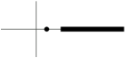
Figure 1: The spectrum of $D_{k}H_{k}$ (for small $k$).

The resolvent has a simple pole at $\zeta_{0}$ and is analytic in the complement of $\{\zeta_{0}\}\cup{\mathbb{S}}$. For $k$ larger than $k_{0}$ the spectrum lies in $[b,\infty)$ with $b>0$.

Since the function $V$ in (16) decays exponentially (as $-6e^{-|x|}$) for large $x$ the behavior of the resolvent for $x$ and $y$ large is determined by the functions in the kernel of the constant coefficient operator

$$\zeta-D_{k}(D_{k}+1)$$

obtained by setting $V$ to zero. These are given by $e^{\mu x}$ with $\zeta-(-\mu^{2}+k^{2})(-\mu^{2}+k^{2}+1)=0$ i.e.

$$\mu=\pm\sqrt{{\mathchoice{\textstyle\frac{1}{2}}{\frac{1}{2}}{\frac{1}{2}}{\frac{1}{2}}}+k^{2}\pm{\mathchoice{\textstyle\frac{1}{2}}{\frac{1}{2}}{\frac{1}{2}}{\frac{1}{2}}}\sqrt{1+4\zeta}}.$$

For large times $t$ the main contribution to (20) comes from small $\zeta$. In that domain the eigenvalues are approximately

$$\mu_{1}\approx\sqrt{1+k^{2}+\zeta}$$ (22)

and

$$\mu_{2}\approx\sqrt{k^{2}-\zeta}$$ (23)

and their negatives.

The integration contour in (20) will be chosen as follows. Let first $k\leq k_{0}$. Then

(a) For $k\leq t^{-{\mathchoice{\textstyle\frac{1}{2}}{\frac{1}{2}}{\frac{1}{2}}{\frac{1}{2}}}}$ the contour is as in Figure 2(a).

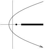
(a) $k\leq t^{-{\mathchoice{\textstyle\frac{1}{2}}{\frac{1}{2}}{\frac{1}{2}}{\frac{1}{2}}}}$

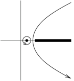
(b) $t^{-{\mathchoice{\textstyle\frac{1}{2}}{\frac{1}{2}}{\frac{1}{2}}{\frac{1}{2}}}}<k<k_{0}$

Figure 2: Integration paths for small values of $k$.

In the neighborhood of the origin the eigenvalues are $\mu_{1}\approx 1$ and $\operatorname{Re}\mu_{2}\approx ct^{-{\mathchoice{\textstyle\frac{1}{2}}{\frac{1}{2}}{\frac{1}{2}}{\frac{1}{2}}}}$ i.e. the decay of the resolvent is a combination of

$$e^{-(1+\mathcal{O}(t^{-{\mathchoice{\textstyle\frac{1}{2}}{\frac{1}{2}}{\frac{1}{2}}{\frac{1}{2}}}}))|x|}\;\;{\rm and}\;\;e^{-\mathcal{O}(t^{-{\mathchoice{\textstyle\frac{1}{2}}{\frac{1}{2}}{\frac{1}{2}}{\frac{1}{2}}}}){|x|}}$$

(b) For $t^{-{\mathchoice{\textstyle\frac{1}{2}}{\frac{1}{2}}{\frac{1}{2}}{\frac{1}{2}}}}\leq k\leq k_{0}$ the contour circles the pole and the semiaxis ${\mathbb{S}}$ as in Figure 2(b). At the pole the eigenvalues are

$$\mu_{1}=1+\mathcal{O}(k^{2}),\;\;\mu_{2}=(1+\mathcal{O}(k^{2}))k.$$

On the second part of the contour and $|\zeta|\leq Ck^{2}$ $\mu_{1}$ is close to 1 and $\mu_{2}$ has real part $\mathcal{O}(k)$ i.e. larger than $t^{-{\mathchoice{\textstyle\frac{1}{2}}{\frac{1}{2}}{\frac{1}{2}}{\frac{1}{2}}}}$.

The resolvent has a representation in terms of the functions in the kernel of ${\mathcal{L}}$ and its adjoint. At $k=\zeta=0$ these are explicit and for small $k$ and $\zeta$ they may be studied perturbatively. We will need explicitly a few of the leading contributions to $K$ for small $k$. The following lemma summarizes this.

Lemma 1.

There exists $k_{0}>0$ such that for all $k<k_{0}$, $t\geq 1$ and all $x,y$ the integral kernel $K(x,y,k,t)$ of the semigroup of the operator $-D_{k}H_{k}$ may be decomposed as

$$K=K_{0}+K_{1}$$ (24)

where

$$K_{0}(x,y,k,t)={\mathchoice{\textstyle\frac{1}{2}}{\frac{1}{2}}{\frac{1}{2}}{\frac{1}{2}}}\partial u_{0}(x)Z(y,k,t)$$ (25)

and

$$K_{1}(x,y,k,t)=\frac{1}{\sqrt{4\pi t}}\Bigl{(}e^{-\frac{(x-y)^{2}}{4t}}-e^{-\frac{(x+y)^{2}}{4t}}\Bigr{)}1_{xy>0}e^{-tk^{2}}+K_{2}(x,y,k,t).$$ (26)

The function $Z$ is even in $y$ and has the property

$$|\int_{\mathbb{R}}Z(y,k,t)\hat{h}(y,k)\mathrm{d}{y}-e^{-{\mathchoice{\textstyle\frac{1}{3}}{\frac{1}{3}}{\frac{1}{3}}{\frac{1}{3}}}tk^{3}}\int_{{\mathbb{R}}^{d}}h(\mathrm{y})\mathrm{d}\mathrm{y}|\leq C\|h\|_{X}t^{-{\mathchoice{\textstyle\frac{1}{3}}{\frac{1}{3}}{\frac{1}{3}}{\frac{1}{3}}}}e^{-{\mathchoice{\textstyle\frac{1}{4}}{\frac{1}{4}}{\frac{1}{4}}{\frac{1}{4}}}tk^{3}}$$ (27)

whereas

$$|K_{2}(x,y,k,t)|\\ \leq\begin{cases}Ct^{-1}e^{-ct^{-{\mathchoice{\textstyle\frac{1}{2}}{\frac{1}{2}}{\frac{1}{2}}{\frac{1}{2}}}}|x-y|}&\text{if $k\leq{t^{-{\mathchoice{\textstyle\frac{1}{2}}{\frac{1}{2}}{\frac{1}{2}}{\frac{1}{2}}}}}$,}\\ C\bigl{(}t^{-1}e^{-{\mathchoice{\textstyle\frac{1}{2}}{\frac{1}{2}}{\frac{1}{2}}{\frac{1}{2}}}tk^{2}-ck|x-y|}+k^{2}e^{-{\mathchoice{\textstyle\frac{1}{4}}{\frac{1}{4}}{\frac{1}{4}}{\frac{1}{4}}}tk^{3}-ck|x-y|}\bigr{)}&\text{if $t^{-{\mathchoice{\textstyle\frac{1}{2}}{\frac{1}{2}}{\frac{1}{2}}{\frac{1}{2}}}}<k<{k_{0}}$.}\end{cases}$$ (28)

We will decompose in the same way also the kernel occurring in eq. (19):

$$S:=(\partial_{y}^{2}-k^{2})K=S_{0}+S_{1}.$$ (29)

The following estimates hold:

Lemma 2.

(a) Let $k\leq t^{-1/2}$ and $t\geq 1$. Then

$$|S_{0}(x,y,k,t)|\leq C(t^{-{\mathchoice{\textstyle\frac{1}{2}}{\frac{1}{2}}{\frac{1}{2}}{\frac{1}{2}}}}e^{-{\mathchoice{\textstyle\frac{1}{2}}{\frac{1}{2}}{\frac{1}{2}}{\frac{1}{2}}}(|x|+|y|)}+t^{-1}e^{-c(|x|+\frac{|y|}{\sqrt{t}})})$$ (30)

and

$$|S_{1}(x,y,k,t)|\leq C(t^{-1}e^{-{\mathchoice{\textstyle\frac{1}{2}}{\frac{1}{2}}{\frac{1}{2}}{\frac{1}{2}}}|x-y|}+t^{-1}e^{-ct^{-1/2}|x|-c|y|}+t^{-3/2}e^{-c\frac{|x-y|}{\sqrt{t}}}).$$ (31)

(b) Let $t^{-1/2}\leq k\leq k_{0}$ and $t\geq 1$. Then

$$\begin{split}|S_{0}(x,y,k,t)|&\leq C(ke^{-{\mathchoice{\textstyle\frac{1}{2}}{\frac{1}{2}}{\frac{1}{2}}{\frac{1}{2}}}(|x|+|y|)}+k^{2}e^{-{\mathchoice{\textstyle\frac{1}{2}}{\frac{1}{2}}{\frac{1}{2}}{\frac{1}{2}}}|x|-ck|y|})e^{-{\mathchoice{\textstyle\frac{1}{4}}{\frac{1}{4}}{\frac{1}{4}}{\frac{1}{4}}}tk^{3}}\\ &\quad+C(t^{-{\mathchoice{\textstyle\frac{1}{2}}{\frac{1}{2}}{\frac{1}{2}}{\frac{1}{2}}}}e^{-{\mathchoice{\textstyle\frac{1}{2}}{\frac{1}{2}}{\frac{1}{2}}{\frac{1}{2}}}(|x|+|y|)}+t^{-1}e^{-{\mathchoice{\textstyle\frac{1}{2}}{\frac{1}{2}}{\frac{1}{2}}{\frac{1}{2}}}|x|-ck|y|})e^{-{\mathchoice{\textstyle\frac{1}{2}}{\frac{1}{2}}{\frac{1}{2}}{\frac{1}{2}}}tk^{2}}\end{split}$$ (32)

and

$$\begin{split}|S_{1}(x,y,k,t)|&\leq C(k^{4}e^{-ck|x-y|}+k^{3}e^{-ck|x|-c|y|}+k^{2}e^{-{\mathchoice{\textstyle\frac{1}{2}}{\frac{1}{2}}{\frac{1}{2}}{\frac{1}{2}}}|x-y|})e^{-{\mathchoice{\textstyle\frac{1}{4}}{\frac{1}{4}}{\frac{1}{4}}{\frac{1}{4}}}tk^{3}}\\ &\quad+C(t^{-1}e^{-{\mathchoice{\textstyle\frac{1}{2}}{\frac{1}{2}}{\frac{1}{2}}{\frac{1}{2}}}|x-y|}+t^{-1}e^{-ck|x|-c|y|}+t^{-\frac{3}{2}}e^{-ck|x-y|})e^{-{\mathchoice{\textstyle\frac{1}{2}}{\frac{1}{2}}{\frac{1}{2}}{\frac{1}{2}}}tk^{2}}.\end{split}$$ (33)

Remark.

In order to get a feeling for the various terms, the following intuition is useful. For large $t$ and $x$ and for small $k$ the resolvent is built out of functions that decay approximately as $e^{-|x|}$, $e^{-k|x|}$ and $e^{-t^{-{\mathchoice{\textstyle\frac{1}{2}}{\frac{1}{2}}{\frac{1}{2}}{\frac{1}{2}}}}|x|}$. Each $x$ derivative brings a factor of $1$, $k$ and $t^{-{\mathchoice{\textstyle\frac{1}{2}}{\frac{1}{2}}{\frac{1}{2}}{\frac{1}{2}}}}$ respectively. Thus, e.g. the third term in (31) behaves as the second derivate of $e^{t\mathop{\triangle}\nolimits}$.

Finally, the large $k$ or short time behavior of the semigroup is dominated by the fourth derivatives in the symbol:

Lemma 3.

(a) Let $k>k_{0}$ and $t>1$. Then

$$|K(x,y,k,t)|,\;\;|S(x,y,k,t)|\leq Ce^{-{\mathchoice{\textstyle\frac{1}{2}}{\frac{1}{2}}{\frac{1}{2}}{\frac{1}{2}}}k^{4}t}e^{-c|x-y|}$$ (34)

(b) Let $t<1$. Then for all $k$

$$|K(x,y,k,t)|\leq Ce^{-{\mathchoice{\textstyle\frac{1}{2}}{\frac{1}{2}}{\frac{1}{2}}{\frac{1}{2}}}k^{4}t}t^{-{\frac{1}{4}}}e^{-{{t}^{-{\mathchoice{\textstyle\frac{1}{4}}{\frac{1}{4}}{\frac{1}{4}}{\frac{1}{4}}}}|x-y|}}.$$ (35)

and

$$|S(x,y,k,t)|\leq Ce^{-{\mathchoice{\textstyle\frac{1}{2}}{\frac{1}{2}}{\frac{1}{2}}{\frac{1}{2}}}k^{4}t}t^{-{\frac{3}{4}}}e^{-{{t}^{-{\mathchoice{\textstyle\frac{1}{4}}{\frac{1}{4}}{\frac{1}{4}}{\frac{1}{4}}}}|x-y|}}.$$ (36)

3 Proof of the Theorem

We solve (19) using the contraction mapping principle in a suitable Banach space. For each $t\geq 1$ we define the Banach space $X_{t}$ of continuous functions $f:{\mathbb{R}}\times{\mathbb{R}}^{d-1}\to{\mathbb{C}}$ as follows. First, let $m=r-d+1$ ($r$ is defined in (9) so $m>2$) and define

$$\omega(x):=(1+|x|)^{-m}.$$

For $t\geq 1$ let

$$k_{t}=\min\{k,1\}+\frac{1}{\sqrt{t}}$$ (37)

and the same notation is used for any positive real number in place of $k$.

The norm in $X_{t}$ is defined to be

$$\|f\|_{t}:=\sup\limits_{\begin{subarray}{c}x\in{\mathbb{R}}\\ k\geq 0\end{subarray}}\bigl{(}\omega(x)+k_{t}\omega(k_{t}x)\bigr{)}^{-1}(1+k^{3}t)^{n}|f(x,\mathbf{k},t)|$$ (38)

Here $n$ can be taken arbitrary number larger than $\frac{d+1}{3}$. The main estimate is the following

Proposition 1.

There exists a $\delta>0$ such that if the initial data satisfies $|h(\mathrm{x})|\leq\delta(1+|\mathrm{x}|)^{-r}$ then the equation (13) has a unique classical solution $v$ such that, for all $t\geq 1$, $v(t)\in X_{t}$ and

$$\|v(t)-\frac{A}{2}\partial_{x}u_{0}(x)\phi(\mathbf{x},t)\|_{t}\leq C\delta t^{-{\frac{1}{12}}}.$$ (39)

Remark. Since for $\psi\in X_{t}$

$$|\psi(\mathrm{x})|\leq\int\mathrm{d}\mathbf{k}(\omega(x)+k_{t}\omega(k_{t}x))(1+k^{3}t)^{-n}\|\psi\|_{t}\leq Ct^{-{\frac{(d-1)}{3}}}\|\psi\|_{t}$$

the sup norm of $v(t)$ is bounded by $Ct^{-{\frac{d-1}{3}}-\frac{1}{12}}$ and the Theorem follows.

The rest of this section is devoted to the proof of Proposition 1. The proof splits into short times and long times. For short times we have the following lemma (see (9) to recall the definition of $\|\cdot\|_{X}$):

Lemma 4.

There exists a $\delta>0$ such that if the initial data satisfies $|h(\mathrm{x})|\leq\delta(1+|\mathrm{x}|)^{-r}$ then $v(1)\in X_{1}$,

$$\|v(1)\|_{X}\leq C\delta\quad\text{and}\quad\|v(1)\|_{1}\leq C\delta.$$ (40)

Proof.

This is quite standard: the leading symbol of the linearized equation is smoothing and preserves polynomial decay. To prove the second estimate we need to control the large $k$ behavior, in view of the definition of the norm in (38). Here it is more natural to work in the $\mathrm{x}$ representation and derive sufficient estimates for the derivatives. Hence let $X^{(p)}$ be the space of $p$ times continuously differentiable functions ${\mathbb{R}}^{d}\to{\mathbb{C}}$ with the norm

$$\|f\|_{X^{(p)}}:=\max_{|\mu|\leq p}\|\partial_{\mathrm{x}}^{\mu}f\|_{X}$$

where $\mu$ is a multi-index. We proceed to show that if the initial condition is in $X^{(p)}$ after an arbitrarily short time the solution will be in $X^{(p+1)}$.

Write (13) in the form

$$\partial_{t}v=-\mathop{\triangle}\nolimits^{2}v+\mathop{\triangle}\nolimits N(v)$$ (41)

with the initial condition $v(0)=h$ and

$$N(v):={\mathchoice{\textstyle\frac{1}{2}}{\frac{1}{2}}{\frac{1}{2}}{\frac{1}{2}}}\bigl{(}(3u_{0}^{2}-1)v+3u_{0}v^{2}+v^{3}\bigr{)}.$$

This is equivalent to the integral equation (after integration by parts)

$$v(t)=e^{-t\mathop{\triangle}\nolimits^{2}}h+\int_{0}^{t}(\mathop{\triangle}\nolimits e^{-(t-s)\mathop{\triangle}\nolimits^{2}})N(v(s))\,\mathrm{d}{s},$$ (42)

which can be differentiated:

$$\partial_{\mathrm{x}}^{\mu}v(t)=e^{-t\mathop{\triangle}\nolimits^{2}}\partial_{\mathrm{x}}^{\mu}h+\int_{0}^{t}\mathop{\triangle}\nolimits e^{-(t-s)\mathop{\triangle}\nolimits^{2}}\partial_{\mathrm{x}}^{\mu}N(v(s))\,\mathrm{d}s.$$ (43)

From the explicit Fourier integral representation it is easy to see that the integral kernel $G(\mathrm{x},\mathrm{y},t)$ of $e^{-t\mathop{\triangle}\nolimits^{2}}$ satisfies the bound

$$|\partial_{\mathrm{y}}^{\nu}G(\mathrm{x},\mathrm{y},t)|\leq C_{\nu}t^{-\frac{d+|\nu|}{4}}e^{-t^{-1/4}|\mathrm{x}-\mathrm{y}|}$$

for all multi-indices $\nu$ and $\mathrm{x},\mathrm{y}\in{\mathbb{R}}^{d}$. Thus for any $f\in X$

$$\begin{split}|(e^{-t\mathop{\triangle}\nolimits^{2}}f)(\mathrm{x})|&\leq\int_{{\mathbb{R}}^{d}}\frac{C}{t^{d/4}}e^{-\frac{|\mathrm{x}-\mathrm{y}|}{t^{1/4}}}\frac{\|f\|_{X}}{(1+|\mathrm{y}|)^{r}}\,\mathrm{d}\mathrm{y}\\ &\leq C\sup_{\mathrm{y}}e^{-\frac{|\mathrm{x}-\mathrm{y}|}{2t^{1/4}}}\frac{\|f\|_{X}}{(1+|\mathrm{y}|)^{r}}\int_{{\mathbb{R}}^{d}}\frac{1}{t^{d/4}}e^{-\frac{|\mathrm{x}-\mathrm{y}|}{2t^{1/4}}}\,\mathrm{d}\mathrm{y}\leq\frac{C\|f\|_{X}}{(1+|\mathrm{x}|)^{r}}\end{split}$$

when $t\leq 1$ and for any $g\in C([0,1],X)$

$$\begin{split}\int_{0}^{t}\mathop{\triangle}\nolimits e^{-(t-s)\mathop{\triangle}\nolimits^{2}}g(s)\,\mathrm{d}s&\leq\frac{C}{(1+|\mathrm{x}|)^{r}}\sup_{s\in[0,1]}\|g(s)\|_{X}\int_{0}^{t}\frac{1}{(t-s)^{1/2}}\,\mathrm{d}s\\ &\leq\frac{Ct^{1/2}}{(1+|\mathrm{x}|)^{r}}\sup_{s\in[0,1]}\|g(s)\|_{X}.\end{split}$$

It follows that for any small enough $\tau>0$ (42) can be solved by the contraction mapping principle in the Banach space $C([0,\tau],X^{(p)})$ with the maximum norm. Namely, there exists $\delta_{0}>0$ s.t. if $\|h\|_{X^{(p)}}<\delta_{0}$ then $\|v\|_{C([0,\tau],X^{(p)})}\leq C\|h\|_{X^{(p)}}$.

Differentiating (43) yet again yields

$$\partial_{\mathrm{x}_{j}}\partial_{\mathrm{x}}^{\mu}v(t)=\partial_{\mathrm{x}_{j}}e^{-t\mathop{\triangle}\nolimits^{2}}\partial_{\mathrm{x}}^{\mu}h+\int_{0}^{t}\partial_{\mathrm{x}_{j}}\mathop{\triangle}\nolimits e^{-(t-s)\mathop{\triangle}\nolimits^{2}}\partial_{\mathrm{x}}^{\mu}N(v(s))\,\mathrm{d}s.$$

Estimate the integrals as in the previous case to get

$$|\partial_{\mathrm{x}_{j}}\partial_{\mathrm{x}}^{\mu}v(t,{\mathrm{x}})|<\frac{C}{(1+|\mathrm{x}|)^{r}}\Bigl{(}\frac{1}{t^{1/4}}\|\partial_{\mathrm{x}}^{\mu}h\|_{X}+t^{1/4}\sup_{\nu\leq\mu}\|\partial_{\mathrm{x}}^{\nu}v\|_{C([0,\tau],X)}\Bigr{)}.$$

Thus the solution gains another derivative in an arbitrarily short time. This can be iterated to get the estimate $\|v(1)\|_{X^{(3n)}}\leq C\|h\|_{X}$, which proves the lemma. ∎

Let us denote

$$f=v(1)$$

and write our integral equation (19) for $t\geq 1$

$$v(x,\mathbf{k},t)=(e^{(t-1){\mathcal{L}}}f)(x,\mathbf{k})\\ +\int_{1}^{t}\int_{\mathbb{R}}S(x,y,\mathbf{k},t-s)\,\bigl{(}{\tfrac{3}{2}}u_{0}(y)v^{*2}(y,\mathbf{k},s)+{\mathchoice{\textstyle\frac{1}{2}}{\frac{1}{2}}{\frac{1}{2}}{\frac{1}{2}}}v^{*3}(y,\mathbf{k},s)\bigr{)}\mathrm{d}{s}\mathrm{d}{y}$$ (44)

We want to prove that $v(t)$ satisfies the estimate (39). Let us start with the solution of the linear equation:

Lemma 5.

Let $t\geq 1$. The solution to the linearized problem is given by

$$e^{(t-1){\mathcal{L}}}f=v_{0}+v_{1}$$ (45)

$$v_{0}(x,\mathbf{k},t)=\frac{A}{2}\partial u_{0}(x)e^{-{\mathchoice{\textstyle\frac{1}{3}}{\frac{1}{3}}{\frac{1}{3}}{\frac{1}{3}}}tk^{3}}$$ (46)

with $A=\int_{{\mathbb{R}}^{d}}f$ and

$$\|v_{1}\|_{t}\leq Ct^{-{\mathchoice{\textstyle\frac{1}{3}}{\frac{1}{3}}{\frac{1}{3}}{\frac{1}{3}}}}(\|f\|_{X}+\|f\|_{1}).$$ (47)

Proof.

Let first $t\geq 2$ and $k\leq k_{0}$. Using (24) decompose

$$e^{(t-1){\mathcal{L}}}f=K(t-1)f=K_{0}(t-1)f+K_{1}(t-1)f:=w_{0}(t)+w_{1}(t).$$

By (25) and (27)

$$w_{0}(t,x,\mathbf{k})=\frac{A}{2}\partial u_{0}(x)e^{-{\mathchoice{\textstyle\frac{1}{3}}{\frac{1}{3}}{\frac{1}{3}}{\frac{1}{3}}}k^{3}t}+\tilde{w}(x,\mathbf{k},t)$$ (48)

with

$$A=\int_{{\mathbb{R}}^{d}}f(\mathrm{x})\,\mathrm{d}\mathrm{x}$$

and

$$|\tilde{w}(x,\mathbf{k},t)|\leq C\|f\|_{X}t^{-{\mathchoice{\textstyle\frac{1}{3}}{\frac{1}{3}}{\frac{1}{3}}{\frac{1}{3}}}}e^{-{\mathchoice{\textstyle\frac{1}{4}}{\frac{1}{4}}{\frac{1}{4}}{\frac{1}{4}}}k^{3}t}e^{-|x|}$$ (49)

(we used $|\partial u_{0}(x)|\leq 2e^{-|x|}$) whereby

$$\|\tilde{w}\|_{t}\leq Ct^{-{\mathchoice{\textstyle\frac{1}{3}}{\frac{1}{3}}{\frac{1}{3}}{\frac{1}{3}}}}\|f\|_{X}.$$

For $w_{1}$ we use the decomposition of eq. (26) to write

$$w_{1}=w_{11}+w_{12}.$$

Start with the $w_{11}$ and let say $x\geq 0$. This is bounded by

$$|w_{11}(x,\mathbf{k},t)|\leq\frac{e^{-tk^{2}}\|f\|_{1}}{\sqrt{4\pi t}}\int_{0}^{\infty}|e^{-\frac{(x-y)^{2}}{4t}}-e^{-\frac{(x+y)^{2}}{4t}}|(1+y)^{-m}\mathrm{d}{y}.$$ (50)

Divide the integral to $y\leq\sqrt{t}$ and the complement. For the former, $I_{1}$, use

$$|e^{-\frac{(x-y)^{2}}{4t}}-e^{-\frac{(x+y)^{2}}{4t}}|\leq e^{-\frac{x^{2}}{4t}}|e^{\frac{xy}{2t}}-e^{-\frac{xy}{2t}}|\leq{\frac{C}{\sqrt{t}}}e^{-\frac{x^{2}}{8t}}|y|$$

to obtain

$$I_{1} \leq C\|f\|_{1}t^{-1}e^{-\frac{x^{2}}{8t}}e^{-tk^{2}}\leq C\|f\|_{1}t^{-1}e^{-c(kx+{\frac{x^{2}}{t}})}e^{-{\mathchoice{\textstyle\frac{1}{2}}{\frac{1}{2}}{\frac{1}{2}}{\frac{1}{2}}}tk^{2}}$$

$$\leq C\|f\|_{1}t^{-{\mathchoice{\textstyle\frac{1}{2}}{\frac{1}{2}}{\frac{1}{2}}{\frac{1}{2}}}}k_{t}\omega(k_{t}x)e^{-{\mathchoice{\textstyle\frac{1}{2}}{\frac{1}{2}}{\frac{1}{2}}{\frac{1}{2}}}tk^{2}}$$ (51)

where ${\frac{x^{2}}{t}}+tk^{2}\geq 2kx$ and $k_{t}^{-1}\leq\sqrt{t}$ were used. The integral over $y\geq\sqrt{t}$ is bounded by

$$I_{2}=\frac{e^{-tk^{2}}\|f\|_{1}}{\sqrt{4\pi t}}\int_{\sqrt{t}}^{\infty}(e^{-\frac{(x-y)^{2}}{4t}}+e^{-\frac{(x+y)^{2}}{4t}})(1+y)^{-m}\mathrm{d}{y}.$$ (52)

Consider the first term on the RHS. Integrate first over the domain $|x-y|>{\mathchoice{\textstyle\frac{1}{2}}{\frac{1}{2}}{\frac{1}{2}}{\frac{1}{2}}}x$. Since $(1+y)^{-m}\leq t^{-{\mathchoice{\textstyle\frac{1}{2}}{\frac{1}{2}}{\frac{1}{2}}{\frac{1}{2}}}}(1+y)^{-m+1}$ and $m>2$ we may bound this term by

$$\frac{Ce^{-tk^{2}}\|f\|_{1}}{t}e^{-\frac{x^{2}}{16t}}$$ (53)

which can be absorbed to (51). The integral over $|x-y|\leq{\mathchoice{\textstyle\frac{1}{2}}{\frac{1}{2}}{\frac{1}{2}}{\frac{1}{2}}}x$ in turn is bounded by

$$C\|f\|_{1}e^{-tk^{2}}(1+x)^{-m}.$$ (54)

Since $x>{\tfrac{2}{3}}\sqrt{t}$ in this domain we may bound (54) as

$$C\|f\|_{1}e^{-tk^{2}}k_{t}^{2}(k_{t}+k_{t}x)^{-2}(1+x)^{-m+2} \leq C\|f\|_{1}e^{-tk^{2}}k_{t}^{2}(1+k_{t}x)^{-m}$$

$$\leq C\|f\|_{1}t^{-{\mathchoice{\textstyle\frac{1}{2}}{\frac{1}{2}}{\frac{1}{2}}{\frac{1}{2}}}}k_{t}e^{-{\mathchoice{\textstyle\frac{1}{2}}{\frac{1}{2}}{\frac{1}{2}}{\frac{1}{2}}}tk^{2}}(1+k_{t}x)^{-m}.$$ (55)

The second term on the RHS of (52) is bounded by the first one. Thus, altogether, we got

$$|w_{11}|\leq Ct^{-{\mathchoice{\textstyle\frac{1}{3}}{\frac{1}{3}}{\frac{1}{3}}{\frac{1}{3}}}}(\omega(x)+k_{t}\omega(k_{t}x))e^{-{\mathchoice{\textstyle\frac{1}{4}}{\frac{1}{4}}{\frac{1}{4}}{\frac{1}{4}}}tk^{3}}.$$ (56)

For $w_{12}$ we use (28). This estimate, for $k\leq t^{-{\mathchoice{\textstyle\frac{1}{2}}{\frac{1}{2}}{\frac{1}{2}}{\frac{1}{2}}}}$, is readily seen to produce a bound like (56) and, for $k_{0}\geq k\geq t^{-{\mathchoice{\textstyle\frac{1}{2}}{\frac{1}{2}}{\frac{1}{2}}{\frac{1}{2}}}}$ similarly, if we use $ke^{-{\mathchoice{\textstyle\frac{1}{4}}{\frac{1}{4}}{\frac{1}{4}}{\frac{1}{4}}}tk^{3}}\leq Ct^{-{\mathchoice{\textstyle\frac{1}{3}}{\frac{1}{3}}{\frac{1}{3}}{\frac{1}{3}}}}e^{-{\mathchoice{\textstyle\frac{1}{6}}{\frac{1}{6}}{\frac{1}{6}}{\frac{1}{6}}}tk^{3}}$ (and replace in (56) the ${\mathchoice{\textstyle\frac{1}{4}}{\frac{1}{4}}{\frac{1}{4}}{\frac{1}{4}}}$ by ${\mathchoice{\textstyle\frac{1}{6}}{\frac{1}{6}}{\frac{1}{6}}{\frac{1}{6}}}$).

Thus, altogether, in the domain $k\leq k_{0}$, we have proved the decomposition (45) with

$$|v_{1}(x,\mathbf{k},t)|\leq Ct^{-{\mathchoice{\textstyle\frac{1}{3}}{\frac{1}{3}}{\frac{1}{3}}{\frac{1}{3}}}}(\omega(x)+k_{t}\omega(k_{t}x))e^{-{\mathchoice{\textstyle\frac{1}{6}}{\frac{1}{6}}{\frac{1}{6}}{\frac{1}{6}}}tk^{3}}.$$ (57)

For $t\geq 2$ and $k>k_{0}$ (34) gives

$$|(e^{(t-1){\mathcal{L}}}f)(x,\mathbf{k})|\leq C\|f\|_{1}e^{-{\mathchoice{\textstyle\frac{1}{2}}{\frac{1}{2}}{\frac{1}{2}}{\frac{1}{2}}}k^{4}(t-1)}\omega(x)\leq C\|f\|_{1}e^{-ct}e^{-{\mathchoice{\textstyle\frac{1}{4}}{\frac{1}{4}}{\frac{1}{4}}{\frac{1}{4}}}(t-1)k^{3}}\omega(x)$$ (58)

upon using $\int e^{-|x-y|}\omega(y)\mathrm{d}{y}\leq C\omega(x)$. Since

$$\|A\partial u_{0}e^{-{\mathchoice{\textstyle\frac{1}{3}}{\frac{1}{3}}{\frac{1}{3}}{\frac{1}{3}}}tk^{3}}1_{k>k_{0}}\|_{t}\leq\|f\|e^{-ct}$$

it can be absorbed into (47).

For $t\leq 2$ use (35) and (70):

$$|(e^{(t-1){\mathcal{L}}}f)(x)|\leq\frac{C\|f\|_{1}}{(1+k^{3})^{n}(t-1)^{1/4}}\int_{\mathbb{R}}e^{-\frac{|x-y|}{(t-1)^{1/4}}}\omega(y)\,\mathrm{d}y\leq\frac{C\|f\|_{1}\omega(x)}{(1+k^{3})^{n}}.$$

Again this and $v_{0}$ can be absorbed into $v_{1}$. ∎

Define next $w=v-e^{(t-1){\mathcal{L}}}$ and $w_{1}=w+v_{1}$, i.e.,

$$v=v_{0}+w_{1}=v_{0}+v_{1}+w.$$

We show that $w$ and $w_{1}$ remain bounded in the Banach space ${\mathcal{B}}$ of continuous functions $s\to w(s)\in X_{s}$ with norm

$$\|w\|:=\sup_{s\geq 1}s^{\frac{1}{12}}\|w(\cdot,\cdot,s)\|_{s}.$$ (59)

Proposition 1 follows since $v=v_{0}+w_{1}$.

Assume now that $t>2$. Since the estimates for our semigroup are quite different for short and long times, we decompose the integral equation as

$$w(t) =\int_{1}^{t-1}S(t-s)({\tfrac{3}{2}}u_{0}(v_{0}(s)+w_{1}(s))^{*2}+{\mathchoice{\textstyle\frac{1}{2}}{\frac{1}{2}}{\frac{1}{2}}{\frac{1}{2}}}v(s)^{*3})\,\mathrm{d}{s}+C(t)$$ (60)

$$C(t) =\int_{t-1}^{t}S(t-s)({\tfrac{3}{2}}u_{0}v(s)^{*2}+{\mathchoice{\textstyle\frac{1}{2}}{\frac{1}{2}}{\frac{1}{2}}{\frac{1}{2}}}v(s)^{*3})\,\mathrm{d}{s};$$ (61)

for later convenience we wrote in the first term $v=v_{0}+w_{1}$. (We omit the details of the case $1<t\leq 2$. This is simpler: one omits the term with $\int_{1}^{t-1}$ on the right hand side of (60), and the integral in (61) is replaced by $\int_{1}^{t}$. One applies the estimates given for $C(t)$ below.)

We assume that (40) holds and that $w$ is in the ball with radius $\delta$ at the origin of ${\mathcal{B}}$ and show the RHS of (60) stays in this ball and contracts there. Then (39) follows from the contraction mapping principle. Notice that $v$ satisfies by (46), (47) and (59)

$$\sup_{s\leq t}\|v(\cdot,\cdot,s)\|_{s}\leq C\delta$$ (62)

since $|A|\leq C\delta$.

Next, recall that for $t-s>1$ we have the decomposition $S=S_{0}+S_{1}$ where the operator $S_{0}$ annihilates odd functions since $Z$ in (25) is even. Since $u_{0}$ is odd and $v_{0}$ even, the term involving $S_{0}u_{0}v_{0}^{*2}$ vanishes and we may rewrite (60) as

$$w(t) =\int_{1}^{t-1}S_{0}(t-s)({\tfrac{3}{2}}u_{0}(v_{0}+w_{1})*w_{1}+{\mathchoice{\textstyle\frac{1}{2}}{\frac{1}{2}}{\frac{1}{2}}{\frac{1}{2}}}v^{*3})\,\mathrm{d}{s}$$

$$\quad+\int_{1}^{t-1}S_{1}(t-s)({\tfrac{3}{2}}u_{0}v^{*2}+{\mathchoice{\textstyle\frac{1}{2}}{\frac{1}{2}}{\frac{1}{2}}{\frac{1}{2}}}v^{*3})\,\mathrm{d}{s}+C(t)$$

$$=:A(t)+B(t)+C(t).$$ (63)

We need a lemma about how our norm behaves under convolutions:

Lemma 6.

Let $f,g\in X_{s}$. Then

$$\|f*g\|_{s}\leq Cs^{-{\frac{d-1}{3}}}\|f\|_{s}\|g\|_{s}$$ (64)

Proof.

We get from the definition of the norm (using the notation of (37) )

$$\begin{split}|(f*g)(x,\mathbf{k})|\leq\|f\|_{s}\|g\|_{s}\int_{{\mathbb{R}}^{d-1}}&\bigl{(}\omega(x)+|\mathbf{k}-\mathbf{p}|_{s}\omega(|\mathbf{k}-\mathbf{p}|_{s}x)\bigr{)}\\ &\cdot\bigl{(}\omega(x)+p_{s}\omega(p_{s}x)\bigr{)}\\ &\cdot(1+|\mathbf{k}-\mathbf{p}|^{3}s)^{-n}(1+p^{3}s)^{-n}\,\mathrm{d}\mathbf{p}.\end{split}$$ (65)

Expanding the product the integral gives rise to four contributions. Three of these have at least one factor $\omega(x)$ and can be estimated by $C\omega(x)I$, where

$$I:=\int(1+|\mathbf{k}-\mathbf{p}|^{3}s)^{-n}(1+p^{3}s)^{-n}\mathrm{d}\mathbf{p}.$$ (66)

Dividing the integration domain to $E:=\{|\mathbf{p}-\mathbf{k}|\leq{\mathchoice{\textstyle\frac{1}{2}}{\frac{1}{2}}{\frac{1}{2}}{\frac{1}{2}}}k\}$ and the complement $E_{c}$, we estimate

$$I \leq(1+({\mathchoice{\textstyle\frac{1}{2}}{\frac{1}{2}}{\frac{1}{2}}{\frac{1}{2}}}k)^{3}s)^{-n}\Bigl{(}\int_{E}(1+|\mathbf{k}-\mathbf{p}|^{3}s)^{-n}\,\mathrm{d}\mathbf{p}+\int_{E_{c}}(1+p^{3}s)^{-n}\,\mathrm{d}\mathbf{p}\Bigr{)}$$

$$\leq C(1+k^{3}s)^{-n}\int_{{\mathbb{R}}^{d-1}}(1+p^{3}s)^{-n}\,\mathrm{d}\mathbf{p}\leq C(1+k^{3}s)^{-n}s^{-{\frac{d-1}{3}}}.$$ (67)

The remaining term $I^{\prime}$ is more complicated:

$$I^{\prime} :=\int p_{s}|\mathbf{k}-\mathbf{p}|_{s}\omega(p_{s}x)\omega(|\mathbf{k}-\mathbf{p}|_{s}x)(1+|\mathbf{k}-\mathbf{p}|^{3}s)^{-n}(1+p^{3}s)^{-n}\,\mathrm{d}\mathbf{p}$$

$$\leq Ck_{s}\omega(k_{s}x)(1+k^{3}s)^{-n}\int_{E}\omega(|\mathbf{k}-\mathbf{p}|_{s}x)(1+|\mathbf{k}-\mathbf{p}|^{3}s)^{-n}\,\mathrm{d}\mathbf{p}$$

$$\quad+C\omega(k_{s}x)(1+k^{3}s)^{-n}\int_{E_{c}}p_{s}|\mathbf{k}-\mathbf{p}|_{s}\omega(p_{s}x)(1+p^{3}s)^{-n}\mathrm{d}\mathbf{p}.$$

The first term is of the appropriate form, since the integral is bounded by $Cs^{-(d-1)/3}$. We need to extract a $k_{s}$ also from the second integral. Use $|\mathbf{k}-\mathbf{p}|_{s}\leq k_{s}+p_{s}$. The term containing $k_{s}$ is clear, and it remains to estimate

$$\int_{E_{c}}p_{s}^{2}\omega(p_{s}x)(1+p^{3}s)^{-n}\mathrm{d}\mathbf{p} \leq\int_{{\mathbb{R}}^{d-1}}\Bigl{(}p+\frac{1}{\sqrt{s}}\Bigr{)}^{2}(1+p^{3}s)^{-n}\mathrm{d}\mathbf{p}$$

$$\leq\frac{C}{s^{(d+1)/3}}\leq\frac{Ck_{s}}{s^{(d-1)/3}}.$$

∎

Let us start bounding the terms in (63) and consider first $C(t)$. By Lemma 6 and (62) we have

$$\|v^{*2}\|_{s}\;,\;\|v^{*3}\|_{s}\leq C\delta^{2}s^{-{\frac{d-1}{3}}}.$$ (68)

Thus the bound (36) gives

$$|C(t)|\leq C\delta^{2}\int_{t-1}^{t}\mathrm{d}{s}\,e^{-{\mathchoice{\textstyle\frac{1}{2}}{\frac{1}{2}}{\frac{1}{2}}{\frac{1}{2}}}k^{4}(t-s)}(t-s)^{-{\frac{3}{4}}}\int\mathrm{d}{y}\,e^{-{{(t-s)}^{-{\mathchoice{\textstyle\frac{1}{4}}{\frac{1}{4}}{\frac{1}{4}}{\frac{1}{4}}}}|x-y|}}\\ \cdot(\omega(y)+k_{s}\omega(k_{s}y))(1+sk^{3})^{-n}s^{-{\frac{d-1}{3}}}.$$ (69)

The following simple estimate is needed repeatedly below:

Lemma 7.

Let $k,p>0$. Then

$$\int\mathrm{d}ye^{-k|x-y|}\omega(py)\leq\begin{cases}Ck^{-1}\omega(px)&\text{\ for $k>p$,}\\ C(p^{-1}\omega(kx)+k^{-1}\omega(px))&\text{\ for $k\leq p$.}\end{cases}$$ (70)

Proof.

For $k>p$ we decompose the integral to the set $E$ given by $|x-y|\leq{\mathchoice{\textstyle\frac{1}{2}}{\frac{1}{2}}{\frac{1}{2}}{\frac{1}{2}}}|x|$ and its complement $E_{c}$:

$$\int e^{-k|x-y|}\omega(py)\,\mathrm{d}y\leq\omega({\mathchoice{\textstyle\frac{1}{2}}{\frac{1}{2}}{\frac{1}{2}}{\frac{1}{2}}}px)\int_{E}e^{-k|x-y|}\,\mathrm{d}y+e^{-{\mathchoice{\textstyle\frac{1}{4}}{\frac{1}{4}}{\frac{1}{4}}{\frac{1}{4}}}p|x|}\int_{E_{c}}e^{-{\mathchoice{\textstyle\frac{1}{2}}{\frac{1}{2}}{\frac{1}{2}}{\frac{1}{2}}}k|x-y|}\omega(py)\,\mathrm{d}y$$

and (70) follows. ∎

Using Lemma 7 and $e^{-(t-s)^{-1/4}|x-y|}\leq e^{-|x-y|}$ we may now bound the $y$ integral in (69) by

$$\int\mathrm{d}{y}e^{-|x-y|}(\omega(y)+k_{s}\omega(k_{s}y))\leq C(\omega(x)+k_{s}\omega(k_{s}x))$$

Since $s\in[t-1,t]$, by changing the constant $C$ we may replace $s$ by $t$ except in the $t-s$ factors and end up with

$$|C(t)|\leq C\delta^{2}t^{-{\frac{d-1}{3}}}(\omega(x)+k_{t}\omega(k_{t}x))(1+tk^{3})^{-n}$$

i.e. the ${\mathcal{B}}_{t}$ norm is bounded by

$$\|C(t)\|_{t}\leq C\delta^{2}t^{-{\frac{d-1}{3}}}$$ (71)

For $A$ and $B$ in (63) we need to distinguish between the various $k$ values.

(a). Let first $k\leq t^{-{\mathchoice{\textstyle\frac{1}{2}}{\frac{1}{2}}{\frac{1}{2}}{\frac{1}{2}}}}$. Using (68) and (31) we bound $B(t)$ by

$$|B(t)| \leq C\delta^{2}(I_{1}+I_{2}+I_{3})$$

$$I_{1} :=\int_{1}^{t-1}\mathrm{d}{s}\int\mathrm{d}{y}\,(t-s)^{-1}e^{-{\mathchoice{\textstyle\frac{1}{2}}{\frac{1}{2}}{\frac{1}{2}}{\frac{1}{2}}}|x-y|}s^{-{\frac{d-1}{3}}}(\omega(y)+k_{s}\omega(k_{s}y))$$ (72)

$$I_{2} :=\int_{1}^{t-1}\mathrm{d}{s}\int\mathrm{d}{y}\,(t-s)^{-1}e^{-c\frac{|x|}{\sqrt{t-s}}-c|y|}s^{-{\frac{d-1}{3}}}(\omega(y)+k_{s}\omega(k_{s}y))$$ (73)

$$I_{3} :=\int_{1}^{t-1}\mathrm{d}{s}\int\mathrm{d}{y}\,(t-s)^{-3/2}e^{-c\frac{|x-y|}{\sqrt{t-s}}}s^{-{\frac{d-1}{3}}}(\omega(y)+k_{s}\omega(k_{s}y))$$ (74)

For $I_{1}$ we use Lemma 7, $s^{-1/2}<k_{s}<2s^{-1/2}$ and $\omega(x/\sqrt{s})\leq\omega(x/\sqrt{t})$ to deduce

$$I_{1} \leq C\int_{1}^{t-1}\mathrm{d}{s}\,(t-s)^{-1}s^{-{\frac{d-1}{3}}}\Bigl{(}\omega(x)+\frac{1}{\sqrt{s}}\omega(\frac{x}{\sqrt{s}})\Bigr{)}$$

$$\leq\frac{C\log t}{t^{{\frac{1}{3}}}}\Bigl{(}\omega(x)+k_{t}\omega(k_{t}x)\Bigr{)}.$$ (75)

For $I_{2}$ we use simply

$$I_{2}\leq\int_{1}^{t-1}\frac{\mathrm{d}{s}}{(t-s)s^{{\frac{d-1}{3}}}}\omega(\frac{x}{\sqrt{t}})\leq\frac{C\log t}{t^{{\frac{d-1}{3}}}}\omega(\frac{x}{\sqrt{t}}),$$

assuming $d\leq 4$. (The bound is not useful in the case $d=2$.) For all $d\geq 3$ we obtain $I_{2}\leq Ct^{-1/6}\log t\ k_{t}\omega(k_{t}x)$.

For $I_{3}$ we use Lemma 7 again, then estimate both $\omega(x/\sqrt{s})$ and $\omega(x/\sqrt{t-s})$ by $\omega(x/\sqrt{t})$:

$$I_{3} \leq C\int_{1}^{t-1}\mathrm{d}{s}\,s^{-{\frac{d-1}{3}}}(t-s)^{-3/2}\Bigl{(}\omega(\frac{x}{\sqrt{t-s}})+\sqrt{t-s}\omega(x)+\sqrt{\frac{t-s}{s}}\omega(\frac{x}{\sqrt{s}})\Bigr{)}$$

$$\leq\frac{C}{t^{\frac{d-1}{3}}}\Bigl{(}\omega(x)\log t+\omega(\frac{x}{\sqrt{t}})\Bigr{)}+\frac{C\log t}{t^{5/6}}\omega(\frac{x}{\sqrt{t}}))$$ (76)

for $d\leq 4$. Again for $d=2$ the result is not useful. For $d>4$ one obtains $I_{3}\leq Ct^{-1}(\omega(x)+\omega(x/\sqrt{t}))$. Thus for $d\geq 3$,

$$|B(t)|\leq C\delta^{2}t^{-1/6}\log t\;\Bigl{(}\omega(x)+t^{-{\mathchoice{\textstyle\frac{1}{2}}{\frac{1}{2}}{\frac{1}{2}}{\frac{1}{2}}}}\omega(\frac{x}{\sqrt{t}})\Bigr{)}.$$ (77)

For the $A(t)$ in (63) we use Lemma 6 to bound

$$\|{\tfrac{3}{2}}u_{0}(v_{0}+w_{1})*w_{1}+{\mathchoice{\textstyle\frac{1}{2}}{\frac{1}{2}}{\frac{1}{2}}{\frac{1}{2}}}v^{*3}\|_{s}\leq C\delta^{2}(s^{-{\frac{d-1}{3}}-\frac{1}{12}}+s^{-2{\frac{d-1}{3}}})\leq C^{\prime}\delta^{2}s^{-{\frac{d-1}{3}}-\frac{1}{12}}$$

and then (30) to get the bound

$$\begin{split}C\delta^{2}\int_{1}^{t-1}\mathrm{d}{s}\,&\bigl{(}(t-s)^{-{\mathchoice{\textstyle\frac{1}{2}}{\frac{1}{2}}{\frac{1}{2}}{\frac{1}{2}}}}e^{-{\mathchoice{\textstyle\frac{1}{2}}{\frac{1}{2}}{\frac{1}{2}}{\frac{1}{2}}}(|x|+|y|)}+(t-s)^{-1}e^{-c(|x|+(t-s)^{-{\mathchoice{\textstyle\frac{1}{2}}{\frac{1}{2}}{\frac{1}{2}}{\frac{1}{2}}}}|y|)}\bigr{)}\\ &\cdot s^{-{\frac{d-1}{3}}-\frac{1}{12}}(\omega(y)+k_{s}\omega(k_{s}y))\end{split}$$

which for $d\geq 3$ is bounded by

$$C\delta^{2}t^{-{\mathchoice{\textstyle\frac{1}{6}}{\frac{1}{6}}{\frac{1}{6}}{\frac{1}{6}}}}\omega(x).$$ (78)

Thus for $k\leq t^{-{\mathchoice{\textstyle\frac{1}{2}}{\frac{1}{2}}{\frac{1}{2}}{\frac{1}{2}}}}$

$$|A(t)+B(t)|\leq C\delta^{2}\log t\;t^{-1/6}\Bigl{(}\omega(x)+t^{-{\mathchoice{\textstyle\frac{1}{2}}{\frac{1}{2}}{\frac{1}{2}}{\frac{1}{2}}}}\omega(\frac{x}{\sqrt{t}})\Bigr{)}.$$ (79)

(b)Let us next consider $k\in[t^{-{\mathchoice{\textstyle\frac{1}{2}}{\frac{1}{2}}{\frac{1}{2}}{\frac{1}{2}}}},k_{0}]$ and start again with the $B(t)$ in (63). Using (33) $|B(t)|$ is bounded by the sum of

$$C\delta^{2}\int\limits_{1}^{t-1}\mathrm{d}s\int\mathrm{d}y\,\bigl{(}(t-s)^{-1}e^{-{\mathchoice{\textstyle\frac{1}{2}}{\frac{1}{2}}{\frac{1}{2}}{\frac{1}{2}}}|x-y|}+(t-s)^{-1}e^{-ck|x|-c|y|}+(t-s)^{-3/2}e^{-ck|x-y|}\bigr{)}\\ \cdot s^{-{\frac{d-1}{3}}}\bigl{(}\omega(y)+k_{s}\omega(k_{s}y)\bigr{)}e^{-{\mathchoice{\textstyle\frac{1}{2}}{\frac{1}{2}}{\frac{1}{2}}{\frac{1}{2}}}(t-s)k^{2}}(1+sk^{3})^{-n}$$ (80)

and

$$C\delta^{2}\int_{1}^{t-1}\mathrm{d}{s}\int\mathrm{d}{y}\,\bigl{(}k^{4}e^{-ck|x-y|}+k^{3}e^{-c(k|x|+|y|)}+k^{2}e^{-{\mathchoice{\textstyle\frac{1}{2}}{\frac{1}{2}}{\frac{1}{2}}{\frac{1}{2}}}|x-y|}\bigr{)}\\ \cdot s^{-{\frac{d-1}{3}}}\bigl{(}\omega(y)+k_{s}\omega(k_{s}y)\bigr{)}e^{-{\mathchoice{\textstyle\frac{1}{4}}{\frac{1}{4}}{\frac{1}{4}}{\frac{1}{4}}}(t-s)k^{3}}(1+sk^{3})^{-n}.$$ (81)

The first integral resembles the case $k<t^{-1/2}$. To estimate (80) use

$$e^{-{\mathchoice{\textstyle\frac{1}{2}}{\frac{1}{2}}{\frac{1}{2}}{\frac{1}{2}}}(t-s)k^{2}}(1+sk^{3})^{-n}\leq C(1+tk^{3})^{-n},$$

and assume $d\leq 4$. Then (80) is bounded by

$$C\delta^{2}(1+tk^{3})^{-n}\int\limits_{1}^{t-1}\mathrm{d}{s}\,\frac{1}{s^{{\frac{d-1}{3}}}(t-s)}\Bigl{(}\omega(x)+\omega(kx)+\frac{1}{k\sqrt{t-s}}(\omega(x)+k_{s}\omega(k_{s}x))\Bigr{)}\\ \leq C\delta^{2}(1+tk^{3})^{-n}\Bigl{(}\frac{\log t}{t^{{\frac{d-1}{3}}}}(\omega(x)+\omega(k_{t}x))+\frac{1}{t^{{\frac{d-1}{3}}}}(\sqrt{t}\omega(x)+\omega(k_{t}x))\Bigr{)}.$$ (82)

In the case $d>4$ replace $(d-1)/3$ by $1$. For $d\geq 3$ we thus get the bound

$$C\delta^{2}(1+tk^{3})^{-n}\frac{\log t}{t^{1/6}}(\omega(x)+k_{t}\omega(k_{t}x)).$$ (83)

Thus (81) remains. Using (70) we have

$$\int e^{-{\mathchoice{\textstyle\frac{1}{2}}{\frac{1}{2}}{\frac{1}{2}}{\frac{1}{2}}}k|x-y|}\omega(y)\mathrm{d}{y}\leq C(k^{-1}\omega(x)+\omega(kx))$$

and

$$\int e^{-{\mathchoice{\textstyle\frac{1}{2}}{\frac{1}{2}}{\frac{1}{2}}{\frac{1}{2}}}k|x-y|}k_{s}\omega(k_{s}y)\mathrm{d}{y}\leq C(k^{-1}k_{s}\omega(k_{s}x)+\omega(kx))$$

whereby

$$\int\mathrm{d}{y}\,\bigl{(}k^{4}e^{-ck|x-y|}+k^{3}e^{-c(k|x|+|y|)}+k^{2}e^{-{\mathchoice{\textstyle\frac{1}{2}}{\frac{1}{2}}{\frac{1}{2}}{\frac{1}{2}}}|x-y|}\bigr{)}\bigl{(}\omega(y)+k_{s}\omega(k_{s}y)\bigr{)}\\ \leq Ck^{2}\bigl{(}\omega(x)+k_{s}\omega(k_{s}x)+k\omega(kx)\bigr{)}\leq Ck^{2}\bigl{(}\omega(x)+(k_{t}+s^{-{\mathchoice{\textstyle\frac{1}{2}}{\frac{1}{2}}{\frac{1}{2}}{\frac{1}{2}}}})\omega(k_{t}x)\bigr{)}$$

since $\omega(kx)$ and $\omega(k_{s}x)$ are bounded by $C\omega(k_{t}x)$ for $k>t^{-1/2}$. Thus

$$\eqref{int3}\leq C\delta^{2}\int_{1}^{t-1}\mathrm{d}{s}\,s^{-{\frac{d-1}{3}}}e^{-{\mathchoice{\textstyle\frac{1}{4}}{\frac{1}{4}}{\frac{1}{4}}{\frac{1}{4}}}(t-s)k^{3}}(1+sk^{3})^{-n}k^{2}\bigl{(}\omega(x)+(k_{t}+s^{-{\mathchoice{\textstyle\frac{1}{2}}{\frac{1}{2}}{\frac{1}{2}}{\frac{1}{2}}}})\omega(k_{t}x)\bigr{)}.$$

Using

$$e^{-{\mathchoice{\textstyle\frac{1}{4}}{\frac{1}{4}}{\frac{1}{4}}{\frac{1}{4}}}(t-s)k^{3}}(1+sk^{3})^{-n}k^{2}\leq C(t-s)^{-2/3}(1+tk^{3})^{-n}$$

we get

$$\eqref{int3}\leq C\delta^{2}(\omega(x)+k_{t}\omega(k_{t}x))(1+tk^{3})^{-n}\int_{1}^{t-1}\mathrm{d}{s}\,s^{-{\frac{d-1}{3}}}(t-s)^{-2/3}\Bigl{(}1+({\frac{t}{s}})^{\mathchoice{\textstyle\frac{1}{2}}{\frac{1}{2}}{\frac{1}{2}}{\frac{1}{2}}}\Bigr{)}.$$

The integral is, for $d=3$, bounded by $Ct^{-{\mathchoice{\textstyle\frac{1}{6}}{\frac{1}{6}}{\frac{1}{6}}{\frac{1}{6}}}}$ and we end up with the bound for $k\in[t^{-{\mathchoice{\textstyle\frac{1}{2}}{\frac{1}{2}}{\frac{1}{2}}{\frac{1}{2}}}},k_{0}]$

$$\eqref{int3}\leq C\delta^{2}t^{-{\mathchoice{\textstyle\frac{1}{6}}{\frac{1}{6}}{\frac{1}{6}}{\frac{1}{6}}}}(\omega(x)+k_{t}\omega(k_{t}x))(1+tk^{3})^{-n}$$ (84)

$A(t)$ in (63) is for $k\in[t^{-{\mathchoice{\textstyle\frac{1}{2}}{\frac{1}{2}}{\frac{1}{2}}{\frac{1}{2}}}},k_{0}]$ bounded by the sum of

$$C\delta^{2}\int\mathrm{d}{y}\int_{1}^{t-1}\mathrm{d}{s}\,\bigl{(}k^{2}e^{-{\mathchoice{\textstyle\frac{1}{2}}{\frac{1}{2}}{\frac{1}{2}}{\frac{1}{2}}}|x|-ck|y|}+ke^{-{\mathchoice{\textstyle\frac{1}{2}}{\frac{1}{2}}{\frac{1}{2}}{\frac{1}{2}}}(|x|+|y|)}\bigr{)}\\ \cdot s^{-{\frac{d-1}{3}}}s^{-1/12}(\omega(y)+k_{s}\omega(k_{s}y))e^{-{\mathchoice{\textstyle\frac{1}{4}}{\frac{1}{4}}{\frac{1}{4}}{\frac{1}{4}}}(t-s)k^{3}}(1+sk^{3})^{-n}$$ (85)

and

$$C\delta^{2}\int\mathrm{d}{y}\int_{1}^{t-1}\mathrm{d}{s}\,\bigl{(}(t-s)^{-{\mathchoice{\textstyle\frac{1}{2}}{\frac{1}{2}}{\frac{1}{2}}{\frac{1}{2}}}}e^{-{\mathchoice{\textstyle\frac{1}{2}}{\frac{1}{2}}{\frac{1}{2}}{\frac{1}{2}}}(|x|+|y|)}+(t-s)^{-1}e^{-{\mathchoice{\textstyle\frac{1}{2}}{\frac{1}{2}}{\frac{1}{2}}{\frac{1}{2}}}|x|-ck|y|}\bigr{)}\\ \cdot s^{-{\frac{d-1}{3}}}s^{-1/12}(\omega(y)+k_{s}\omega(k_{s}y))e^{-{\mathchoice{\textstyle\frac{1}{2}}{\frac{1}{2}}{\frac{1}{2}}{\frac{1}{2}}}(t-s)k^{2}}(1+sk^{3})^{-n}$$

In the former expression we replace as above $k$ by $(t-s)^{-1/3}$ and end up with the bound

$$C\delta^{3}t^{-1/12}\omega(x)(1+tk^{3})^{-n}.$$ (86)

and the latter is smaller with $t^{-1/12}$ replaced by $t^{-1/6}$. Thus for $k\in[t^{-{\mathchoice{\textstyle\frac{1}{2}}{\frac{1}{2}}{\frac{1}{2}}{\frac{1}{2}}}},k_{0}]$

$$|A(t)+B(t)|\leq C\delta^{3}t^{-1/12}(\omega(x)+k_{t}\omega(k_{t}x))(1+tk^{3})^{-n}.$$ (87)

(c) Finally we suppose $k>k_{0}$ and use the bound (34) and $\omega(k_{s}x)\leq C\omega(x)$ which holds for such $k$ to get

$$|A(t)+B(t)| \leq C\delta^{2}\int_{1}^{t-1}\mathrm{d}{s}\int\mathrm{d}{y}\,e^{-{\mathchoice{\textstyle\frac{1}{2}}{\frac{1}{2}}{\frac{1}{2}}{\frac{1}{2}}}k^{4}(t-s)}e^{-c|x-y|}s^{-{\frac{d-1}{3}}}\omega(y)(1+sk^{3})^{-n}$$

$$\leq C\delta^{2}t^{-2/3}\omega(x)(1+tk^{3})^{-n}$$ (88)

The bounds (71), (79), (87) and (88) show that our ball is mapped to itself. The contractive property goes similarly.

4 The spectrum

In the remaining sections we will present the linear analysis needed for the semigroup kernel estimates in Lemmas 1, 2 and 3 of Section 2. Since the linearized Cahn–Hilliard operator is of the fourth order, the calculations are lengthy, and we will be brief in the most tedious details. The full details may be found in the thesis [4]. The linear analysis is based on an approach outlined in [6].

We remark that, in addition to the existing notations, boldface letters will mainly refer to vectors in ${\mathbb{C}}^{4}$ and $4\times 4$ matrices in the sequel. A boldface symbol and the corresponding italic symbol are not always mathematically related: consider for example $\mathbf{R}$ and $R$, or $\mathbf{v}$ and $v$.

The following lemma summarizes the properties of the spectrum of $D_{k}H_{k}$ alluded to in Section 2.

Lemma 8.

For any $k>0$ the spectrum of $D_{k}H_{k}$ is contained in $[k^{4},\infty)$. There exists an $\epsilon>0$ such that for $0<k<\epsilon$ the bottom of the spectrum is an isolated eigenvalue $\zeta_{0}$ of multiplicity one with $\zeta_{0}\leq Ck^{3}$. The remaining part of the spectrum is bounded from below by ${\frac{3}{4}}k^{2}$.

Proof.

$D_{k}H_{k}$ has asymptotically constant coefficients, thus the essential spectrum is $[k^{2}+k^{4},\infty)$, the same as that of the constant coefficient limit $D_{k}^{2}+D_{k}$, see [8, Proposition 26.2]. Eigenvalues on the other hand are the same as those of the self-adjoint operator $A_{k}:=D_{k}^{1/2}H_{k}D_{k}^{1/2}$: the eigenvectors are mapped onto each other by $D_{k}^{1/2}$, which is invertible when $k>0$: we have the convolution kernel $(D_{k}^{-1})(x)=:G_{k}(x)=(2k)^{-1}e^{-k|x|}$.

$H_{0}$ has two isolated eigenvalues at $0$ and $3/4$ and a continuous spectrum $[1,\infty)$, see [9, page 79]. The eigenfunctions are $V$ from (16) and $x\mapsto\sinh(x/2)/\cosh(x/2)^{2}$.

The spectrum of $A_{k}$ can be studied with the minimax principle:

$$\zeta_{0}=\inf_{u}\frac{\langle u,H_{k}u\rangle}{\langle u,G_{k}u\rangle}\leq\frac{k^{2}}{\langle V,G_{k}V\rangle}\leq Ck^{3}$$

for small $k$. We also get the lower bound:

$$\zeta_{0}\geq\inf_{u}\frac{k^{4}\|u\|^{2}}{\langle u,k^{2}G_{k}u\rangle}\geq k^{4}.$$

To see that $\zeta_{0}$ is a discrete eigenvalue of multiplicity one we proceed further with the minimax principle:

$$\zeta_{1} =\sup_{v}\inf_{u\in v^{\perp}}\frac{\langle u,A_{k}u\rangle}{\langle u,u\rangle}=\sup_{v}\inf_{\begin{subarray}{c}u\\ \langle G_{k}^{1/2}u,v\rangle=0\end{subarray}}\frac{\langle u,H_{k}u\rangle}{\langle u,G_{k}u\rangle}$$

$$=\sup_{v}\inf_{u\in v^{\perp}}\frac{\langle u,H_{k}u\rangle}{\langle u,G_{k}u\rangle}\geq\sup_{v}\inf_{u\in v^{\perp}}\frac{\langle u,H_{0}u\rangle}{\|u\|^{2}}\frac{k^{2}\|u\|^{2}}{\langle u,k^{2}G_{k}u\rangle}\geq\tfrac{3}{4}k^{2},$$

which for small $k$ is larger than $\zeta_{0}$. Here we used knowledge of the spectrum of $H_{0}$: it has zero and $3/4$ as isolated eigenvalues and a continuous spectrum $[1,\infty)$. ∎

5 The resolvent: a first order system

In Sections 5–8 we analyze the integral kernel of the resolvent of the operator $\zeta-D_{k}H_{k}$, where $\zeta$ is a complex number outside the spectrum of $D_{k}H_{k}$; see (20). We start by writing $(\zeta-D_{k}H_{k})u=f$ as a system of ordinary linear differential equations

$$\mathbf{u}^{\prime}(x)=\mathbf{A}(\zeta,k,x)\mathbf{u}(x)+\mathbf{b}(x),$$ (89)

where

$$\mathbf{u} =(u,u^{\prime},u^{\prime\prime},u^{\prime\prime\prime})^{T}, \mathbf{b} =(0,0,0,-f)^{T}$$ (90)

and (for $V$, see (16) )

$$\mathbf{A}=\begin{pmatrix}0&1&0&0\\ 0&0&1&0\\ 0&0&0&1\\ \zeta-k^{2}-k^{4}-k^{2}V+V^{\prime\prime}&2V^{\prime}&1+2k^{2}+V&0\end{pmatrix}.$$ (91)

We define the $x$-independent matrices $\mathbf{A}_{\infty}(\zeta,k):=\lim_{x\to\pm\infty}\mathbf{A}(\zeta,k,x)$, and $\mathbf{R}(\zeta,k,x):=\mathbf{A}(\zeta,k,x)-\mathbf{A}_{\infty}(\zeta,k)$; the latter can be bounded by $Ce^{-|x|}$ for $(\zeta,k)$ in any compact set. The positive constant $C$ may depend on the set.

The eigenvalues of $\mathbf{A}_{\infty}$ are the zeros of the polynomial

$$\zeta-(-\mu^{2}+k^{2})^{2}-(-\mu^{2}+k^{2})$$

which are

$$\mu_{j}=\pm\sqrt{{\mathchoice{\textstyle\frac{1}{2}}{\frac{1}{2}}{\frac{1}{2}}{\frac{1}{2}}}+k^{2}\pm{\mathchoice{\textstyle\frac{1}{2}}{\frac{1}{2}}{\frac{1}{2}}{\frac{1}{2}}}\sqrt{1+4\zeta}}.$$ (92)

Unfortunately they have somewhat poor analyticity for $k$ and $\zeta$ near zero. This problem can be overcome by writing

$$\zeta=k^{2}+k^{4}+(1+2k^{2})^{2}\tau^{2}$$ (93)

and using $\lambda=(k,\tau)$ as the parameters. Then (91) and (92) become

$$\mathbf{A}=\begin{pmatrix}0&1&0&0\\ 0&0&1&0\\ 0&0&0&1\\ (1+2k^{2})^{2}\tau^{2}-k^{2}V+V^{\prime\prime}&2V^{\prime}&1+2k^{2}+V&0\end{pmatrix}$$

and

$$\mu_{j}=\pm\sqrt{1+2k^{2}}\sqrt{\tfrac{1}{2}\pm\tfrac{1}{2}\sqrt{1+4\tau^{2}}}.$$ (94)

To fix the branches when the second sign is negative, set

$$\pm\sqrt{{\mathchoice{\textstyle\frac{1}{2}}{\frac{1}{2}}{\frac{1}{2}}{\frac{1}{2}}}-{\mathchoice{\textstyle\frac{1}{2}}{\frac{1}{2}}{\frac{1}{2}}{\frac{1}{2}}}\sqrt{1+4\tau^{2}}}=\frac{\pm\mathrm{i}\tau}{\sqrt{{\mathchoice{\textstyle\frac{1}{2}}{\frac{1}{2}}{\frac{1}{2}}{\frac{1}{2}}}+{\mathchoice{\textstyle\frac{1}{2}}{\frac{1}{2}}{\frac{1}{2}}{\frac{1}{2}}}\sqrt{1+4\tau^{2}}}}$$ (95)

and choose $\mu_{2}$ to have the positive sign with the principal branch in the denominator. Now the $\mu_{i}$ are analytic functions of $k$ and $\tau$ when $k\in{\mathbb{C}}\setminus\pm\mathrm{i}[1/\sqrt{2},\infty)$ and $\tau\in{\mathbb{C}}\setminus\pm\mathrm{i}[{\mathchoice{\textstyle\frac{1}{2}}{\frac{1}{2}}{\frac{1}{2}}{\frac{1}{2}}},\infty)$. We are mostly interested in real $k$. Then the cuts in the $\tau$ plane correspond to $\zeta\in(-\infty,-1/4]$, values which we do not need for integrating around the spectrum of $D_{k}H_{k}$. $\tau\in\pm\mathrm{i}[0,{\mathchoice{\textstyle\frac{1}{2}}{\frac{1}{2}}{\frac{1}{2}}{\frac{1}{2}}}k]\cup{\mathbb{R}}$ is mapped onto $[3k^{2}/4-k^{6},\infty)$ which by Lemma 8 contains all of the spectrum of $D_{k}H_{k}$ except for the lowest eigenvalue, which should be somewhere around $\tau\approx\mathrm{i}k$ when $k$ is small. For larger $k$ it is more useful to use the $k^{4}$ bound: $\tau\in\pm\mathrm{i}[0,k/(1+2k^{2})]\cup{\mathbb{R}}$ is mapped onto $[k^{4},\infty)$ which contains the entire spectrum.

The number $\tau$ is mapped two-to-one on $\zeta$ and we will mostly keep $\tau$ in the upper half plane. There $\operatorname{Re}\mu_{2}<0$ when $k$ is real. However, we need some results to be valid also in a small complex neighborhood of the origin for both $k$ and $\tau$, because we will develop a power series there later.

The number $\mu_{1}$ will be the eigenvalue with the most negative real part, $\mu_{4}:=-\mu_{1}$ and $\mu_{3}:=-\mu_{2}$. We have

$$\begin{gathered}\mu_{1}^{2}+\mu_{2}^{2}=1+2k^{2},\qquad\mu_{1}\mu_{2}=-\mathrm{i}\tau(1+2k^{2}),\\ \mu_{1}^{2}-\mu_{2}^{2}=(1+2k^{2})\sqrt{1+4\tau^{2}}=\sqrt{1+4\zeta}.\end{gathered}$$ (96)

We denote by $\mathbf{v}_{j}$ and $\mathbf{w}_{j}$ the right and left eigenvectors of $\mathbf{A}_{\infty}$: $\mathbf{A}_{\infty}\mathbf{v}_{j}=\mu_{j}\mathbf{v}_{j}$ and $\mathbf{w}_{j}\mathbf{A}_{\infty}=\mu_{j}\mathbf{w}_{j}$. The vectors $\mathbf{v}_{j}$ and $\mathbf{w}_{j}$ are easy to express in terms of $\mu_{j}$ and are thus also analytic. Normalize the eigenvectors so that $(\mathbf{v}_{j})_{1}=(\mathbf{w}_{j})_{4}=1$. This results in

$$\mathbf{v}_{j} =\begin{pmatrix}1,&\mu_{j},&\mu_{j}^{2},&\mu_{j}^{3}\end{pmatrix}^{T},$$

$$\mathbf{w}_{j} =\begin{pmatrix}\mu_{j}(\mu_{j}^{2}-1-2k^{2}),&\mu_{j}^{2}-1-2k^{2},&\mu_{j},&1\end{pmatrix}.$$

6 The resolvent: solutions of the homogeneous equations

The resolvent for (89) will be constructed using the solutions of the corresponding homogeneous equation and its transposed equation ($\mathbf{A}(x):=\mathbf{A}(\zeta,k,x)$ and so on):

$$\mathbf{u}^{\prime}(x) =\mathbf{A}(x)\mathbf{u}(x)$$ (97)

$$\mathbf{z}^{\prime}(x) =-\mathbf{z}(x)\mathbf{A}(x).$$ (98)

So, this section contains a study of the solutions of (97) and (98). The motivation for (98) is that if $\mathbf{u}$ and $\mathbf{z}$ are solutions of (97) and (98) the product $\mathbf{z}(x)\mathbf{u}(x)$ is independent of $x$.

As the coefficient matrix $\mathbf{A}(x)$ tends to the constant $\mathbf{A}_{\infty}$ when $x\to\infty$, one would also expect the solutions of (97) and (98) to tend to the solutions of the corresponding constant coefficient equations. Indeed, Pego and Weinstein show in [6] that if there is a simple eigenvalue $\mu_{1}$ with a smaller real part than the other eigenvalues, (97) admits a unique solution $\mathbf{u}_{1}^{+}$ with the property that $e^{-\mu_{1}x}\mathbf{u}_{1}^{+}(x)\to\mathbf{v}_{1}$ as $x\to\infty$. Similarly (98) has an unique solution $\mathbf{z}_{1}^{-}$ with $e^{\mu_{1}x}\mathbf{z}_{1}^{-}(x)\to\mathbf{w}_{1}$ as $x\to-\infty$.

We now examine solutions corresponding to the remaining eigenvalues $\mu_{j}$ for $j\geq 2$. We prove things for $\mathbf{u}^{+}_{j}$ but the $\mathbf{z}^{-}_{j}$ case is similar. Fix a set of values $\lambda:=(k,\tau)\subset{\mathbb{C}}^{2}$ to work with. (As explained in the previous section, the dependence of $\mathbf{A}$ or $\mu_{j}$ on $\lambda$ or $k$ or $\tau$ is analytic in the natural way, if $\lambda$ is restricted to a suitable domain.) Choose some $\lambda$-dependent $\mu$ and substitute $\mathbf{u}(x)=:e^{\mu x}\mathbf{v}(x)$ in (97) to get

$$\mathbf{v}^{\prime}(x)=(\mathbf{B}+\mathbf{R}(x))\mathbf{v}(x),$$ (99)

where $\mathbf{B}:=\mathbf{A}_{\infty}-\mu$ and $\mathbf{R}(x):=\mathbf{A}(x)-\mathbf{A}_{\infty}$.

We want to divide the eigenvalues of $\mathbf{A}_{\infty}$ into two sets: those with smaller real part than $\mu$ and the rest. However, we need some margins in order to keep things uniform in $\lambda$, because the eigenvalues may not maintain the same order for all $\lambda$ (see Section 5).

Let $E_{i}:=\bigcup_{n=1}^{\infty}\ker(\mu_{i}-\mathbf{A}_{\infty})^{n}$. Choose constants $\alpha$ and $\beta$ and a set $I\subset\{1,2,3,4\}$ so that $\operatorname{Re}(\mu_{i}-\mu)\leq\alpha<0$ when $i\in I$ and $\operatorname{Re}(\mu_{i}-\mu)\geq\beta>-\rho$ whenever $i\not\in I$. The numbers $\alpha$ and $\beta$ are assumed independent of $\lambda$. Let $\mathbf{P}$ be the projection onto $\bigoplus_{i\in I}E_{i}$ which commutes with $\mathbf{A}_{\infty}$ and let $\mathbf{Q}:=\mathbf{1}-\mathbf{P}$. Fix some positive $x_{0}$ and define

$$({\mathcal{F}}_{P}\mathbf{v})(x) :=\int_{x_{0}}^{x}e^{(x-{y})\mathbf{B}}\mathbf{P}\mathbf{R}({y})\mathbf{v}({y})\,\mathrm{d}{y},$$ (100)

$$({\mathcal{F}}_{Q}\mathbf{v})(x) :=-\int_{x}^{\infty}e^{(x-{y})\mathbf{B}}\mathbf{Q}\mathbf{R}({y})\mathbf{v}({y})\,\mathrm{d}{y},\ \ \ \ {\mathcal{F}}:={\mathcal{F}}_{P}+{\mathcal{F}}_{Q}$$

for bounded continuous functions $\mathbf{v}:[x_{0},\infty]\to{\mathbb{C}}^{4}$. The proof of the following facts is straightforward:

Lemma 9.

For sufficiently large $x_{0}$, ${\mathcal{F}}$ is a contraction in the norm

$$\|\mathbf{v}\|=\sup_{x\in[x_{0},\infty)}|\mathbf{v}(x)|.$$

Corollary 1.

$({\mathcal{F}}\mathbf{v})(x)=\mathcal{O}(e^{\max(-\rho,\alpha+\epsilon)x})$ for large $x$ and any $\epsilon>0$.

Hence, $\mathbf{v}=\tilde{\mathbf{v}}+{\mathcal{F}}\mathbf{v}$ can be solved for $\mathbf{v}$ given any $\tilde{\mathbf{v}}$. For such a solution

$$(\mathbf{v}-\tilde{\mathbf{v}})^{\prime} =\mathbf{P}\mathbf{R}v+\mathbf{B}{\mathcal{F}}_{P}\mathbf{v}+\mathbf{Q}\mathbf{R}\mathbf{v}+\mathbf{B}{\mathcal{F}}_{Q}\mathbf{v}=\mathbf{B}(\mathbf{v}-\tilde{\mathbf{v}})+\mathbf{R}v.$$

In particular if $\tilde{\mathbf{v}}$ is a bounded solution of $\tilde{\mathbf{v}}^{\prime}=\mathbf{B}\tilde{\mathbf{v}}$ (a constant coefficient equation) for large $x$ then $\mathbf{v}$ will be a solution of (99) with the same asymptotic behavior as $\tilde{\mathbf{v}}$ in the sense that $\mathbf{v}-\tilde{\mathbf{v}}={\mathcal{F}}\mathbf{v}$ tends to zero exponentially fast as $x\to\infty$.

Corollary 2.

For each eigenvalue $\mu_{i}$ there is a solution of (97) which behaves asymptotically (as $x\to\infty$) like $e^{\mu_{i}x}\mathbf{v}_{i}$.

Proof.

Pick $\mu=\mu_{i}$, $\alpha=-\frac{5}{8}$, $\beta=-\tfrac{7}{8}$, $\epsilon=\frac{1}{16}$ and $\tilde{\mathbf{v}}(x)=\mathbf{v}_{i}$. It is clear that a suitable $I$ can be found and ${\mathcal{F}}$ can be used to get a solution for $x>x_{0}$, which can then be extended to the whole real line. ∎

In general the solutions of Corollary 2 are not unique even after fixing normalization of $\mathbf{v}_{i}$ because one can add similar solutions corresponding to $\mu_{j}$ with smaller real parts than $\mu_{i}$.

Corollary 3.

If the $\mu_{i}$ and $\mathbf{v}_{i}$ are analytic functions of $\lambda$ in some domain of ${\mathbb{C}}^{2}$ and we can fix the $I$ in the preceding proof uniformly for all $\lambda$, then the solutions in Corollary 2 are analytic in this domain when evaluated at some fixed $x$. If $\mathbf{u}_{i}$ is such a solution then $|e^{-\mu_{i}(\lambda)x}\mathbf{u}_{i}(\lambda;x)-\mathbf{v}_{i}(\lambda)|<Ce^{-\frac{\rho}{2}x}$ for $x>0$ and $\lambda$ in compact subsets of the domain ($C$ depends on the subset).

By Corollary 2, for $j\in\{1,2,4\}$ there is a $\mathbf{u}^{+}_{j}$ which solves the homogeneous equation $\partial_{x}\mathbf{u}^{+}_{j}=\mathbf{A}\mathbf{u}^{+}_{j}$ and behaves like $e^{\mu_{j}x}\mathbf{v}_{j}$ as $x\to\infty$. There is also a $\mathbf{z}^{-}_{j}$ which solves the transposed equation $\partial_{x}\mathbf{z}^{-}_{j}=-\mathbf{z}^{-}_{j}\mathbf{A}$ and behaves like $e^{-\mu_{j}x}\mathbf{w}_{j}$ as $x\to-\infty$. It would also be possible to define $\mathbf{u}^{+}_{3}$ and $\mathbf{z}^{-}_{3}$ in this way but that would not be very useful because $\mathbf{A}_{\infty}$ is defective at $\tau=0$: the eigenvectors $\mathbf{v}_{2}$ and $\mathbf{v}_{3}$ collide and we would not have a set of four linearly independent solutions. Thus with some abuse of notation we require instead

$$\mathbf{u}^{+}_{3}(x)\sim\frac{e^{\mu_{3}x}\mathbf{v}_{3}-e^{\mu_{2}x}\mathbf{v}_{2}}{\mu_{3}-\mu_{2}}\quad\text{and}\quad\mathbf{z}^{-}_{3}(x)\sim\frac{e^{-\mu_{3}x}\mathbf{w}_{3}-e^{-\mu_{2}x}\mathbf{w}_{2}}{\mu_{3}-\mu_{2}}$$

as $x\to\infty$ and $x\to-\infty$, respectively. As $\mu_{3}-\mu_{2}\to 0$ these converge (pointwise in $x$) to solutions with linear asymptotes.

Our expression for the integral kernel of $(\zeta-D_{k}H_{k})^{-1}$ will contain only $\mathbf{u}^{+}_{j}$ and $\mathbf{z}^{-}_{j}$ for $j\in\{1,2\}$. However, the other two values of $j$ are needed for understanding the behavior of the kernel.

We summarize the properties of the solutions of the homogeneous equations in the following theorem.

Theorem 2.

$$\operatorname{Re}(\mu_{1}\pm\mu_{2})<-\tfrac{5}{8}\quad\text{and}\quad\operatorname{Re}(\mu_{2})<\tfrac{1}{32}.$$ (101)

Then (97) with (91) has solutions $\mathbf{u}^{+}_{i}$ such that $|\mathbf{u}^{+}_{i}(x)-e^{\mu_{i}x}\mathbf{v}_{i}|<C|e^{(\mu_{i}-{\mathchoice{\textstyle\frac{1}{2}}{\frac{1}{2}}{\frac{1}{2}}{\frac{1}{2}}})x}|$ for $i\in\{1,2,4\}$ and

$$|\mathbf{u}^{+}_{3}(x)-\frac{e^{\mu_{3}x}\mathbf{v}_{3}-e^{\mu_{2}x}\mathbf{v}_{2}}{2\mu_{3}}|<C|e^{(\mu_{3}-{\mathchoice{\textstyle\frac{1}{2}}{\frac{1}{2}}{\frac{1}{2}}{\frac{1}{2}}})x}|$$

when $x$ is bounded from below. Furthermore,

$$|\partial_{x}^{n}\mathbf{u}^{+}_{i}(x)-\mu_{i}^{n}e^{\mu_{i}x}\mathbf{v}_{i}| <C|e^{(\mu_{i}-{\mathchoice{\textstyle\frac{1}{2}}{\frac{1}{2}}{\frac{1}{2}}{\frac{1}{2}}})x}|,\qquad n\in\{1,2\},\quad i\neq 3$$

$$|\partial_{x}\mathbf{u}^{+}_{3}(x)-{\mathchoice{\textstyle\frac{1}{2}}{\frac{1}{2}}{\frac{1}{2}}{\frac{1}{2}}}(e^{\mu_{3}x}\mathbf{v}_{3}+e^{\mu_{2}x}\mathbf{v}_{2})| <C|e^{(\mu_{3}-{\mathchoice{\textstyle\frac{1}{2}}{\frac{1}{2}}{\frac{1}{2}}{\frac{1}{2}}})x}|,$$

$$|\partial_{x}^{2}\mathbf{u}^{+}_{3}(x)-{\mathchoice{\textstyle\frac{1}{2}}{\frac{1}{2}}{\frac{1}{2}}{\frac{1}{2}}}(\mu_{3}e^{\mu_{3}x}\mathbf{v}_{3}+\mu_{2}e^{\mu_{2}x}\mathbf{v}_{2})| <C|e^{(\mu_{3}-{\mathchoice{\textstyle\frac{1}{2}}{\frac{1}{2}}{\frac{1}{2}}{\frac{1}{2}}})x}|.$$

Similarly, (98) has solutions $\mathbf{z}^{-}_{i}$ such that $|\mathbf{z}^{-}_{i}(x)-e^{-\mu_{i}x}\mathbf{w}_{i}|<Ce^{({\mathchoice{\textstyle\frac{1}{2}}{\frac{1}{2}}{\frac{1}{2}}{\frac{1}{2}}}-\mu_{i})x}$ for $i\in\{1,2,4\}$ and

$$|\mathbf{z}^{-}_{3}(x)-\frac{e^{-\mu_{3}x}\mathbf{w}_{3}-e^{-\mu_{2}x}\mathbf{w}_{2}}{2\mu_{3}}|<C|e^{({\mathchoice{\textstyle\frac{1}{2}}{\frac{1}{2}}{\frac{1}{2}}{\frac{1}{2}}}-\mu_{3})x}|$$

when $x$ is bounded from above. The corresponding estimates for the derivatives hold.

For $i\in\{1,2,4\}$ the functions $\mathbf{u}^{+}_{i}(x)$ and $\mathbf{z}^{-}_{i}(x)$ are analytic in $\lambda$ wherever the assumptions hold. The functions $\mathbf{u}^{+}_{3}(x)$ and $\mathbf{z}^{-}_{3}(x)$ are continuous and when

$$\operatorname{Re}(\mu_{2})>-\tfrac{1}{4}$$ (102)

also analytic. The constant $C$ above depends on $\lambda$ but can be fixed in any compact subset.

The proof is basically just application of Corollaries 2 and 3 with some additional details for the $i=3$ case. There we need to use different choices for the set $I$ depending whether $\operatorname{Re}(\mu_{2})$ is near zero or not. The results can be glued together with a partition of the unity but analyticity is then lost. See [4] for more details.

Specifying the assumptions in terms of $\mu_{1}$ and $\mu_{2}$ was perhaps a bit opaque. However, there are two cases which interest us. The first is $\lambda\approx 0$. In a small enough neighborhood of the origin both (101) and (102) clearly hold. The second case is when $k$ is real and $\tau$ in the upper half plane. Then $\mu_{2}$ is in the left half plane. For the first inequality of (101) use (96) to get $(\mu_{1}\pm\mu_{2})^{2}=(1+2k^{2})(1\mp 2\mathrm{i}\tau)$. From this we see that the inequality is equivalent to $\tau$ lying beneath an upwards opening parabola with apogee at $\mathrm{i}(128k^{2}+39)/(256k^{2}+128)$. This is always above the values corresponding to the spectrum.

To end this section we still note the following fact, which is a consequence of the symmetry of the Cahn–Hilliard equation under the reflection $x\mapsto-x$:

Lemma 10.

Under the assumptions (101) there are also solutions $\mathbf{u}^{-}_{j}$ and $\mathbf{z}^{+}_{j}$ of (97) and (98), respectively, with prescribed behavior for $x\to-\infty$ and $x\to\infty$: (e.g. $\mathbf{u}^{-}_{1}(x)\sim e^{-\mu_{1}x}\mathbf{v}_{4}$ as $x\to-\infty$). These can be expanded as linear combinations of $\mathbf{u}^{+}_{j}$ and $\mathbf{z}^{-}_{j}$. The coefficients of this expansion are continuous and, when (102) holds, also analytic.

7 The resolvent: a resolvent formula

We now want to write solutions of (89), that is, of $\mathbf{u}^{\prime}=\mathbf{A}\mathbf{u}+\mathbf{b}$, using the solutions of the homogeneous equations. We will use the following resolvent formula:

$$\mathbf{u}(x)=\int_{-\infty}^{x}\mathbf{u}^{+}(x)(\Omega^{+})^{-1}\mathbf{z}^{-}({y})\mathbf{b}({y})\,\mathrm{d}{y}+\int_{\infty}^{x}\mathbf{u}^{-}(x)(\Omega^{-})^{-1}\mathbf{z}^{+}({y})\mathbf{b}({y})\,\mathrm{d}{y},$$ (103)

where $\mathbf{u}^{\pm}=(\mathbf{u}^{\pm}_{1},\mathbf{u}^{\pm}_{2})$, $\mathbf{z}^{\mp}=\left(\begin{smallmatrix}\mathbf{z}_{1}^{\mp}\\ \mathbf{z}_{2}^{\mp}\end{smallmatrix}\right)$ and $\Omega^{\pm}=\mathbf{z}^{\mp}\mathbf{u}^{\pm}$. These products are independent of $x$ and it is also easy to see that $\Omega^{-}=-\Omega^{+}$. For simplicity we will from now on denote $\Omega^{+}$ just by $\Omega$. For (103) to make sense $\Omega$ of course needs to be invertible.

Theorem 3.

Assume $\operatorname{Re}\mu_{1}<\operatorname{Re}\mu_{2}<0$ and $\zeta\in\rho(D_{k}H_{k})$ (the resolvent set). Then $\Omega=\mathbf{z}^{-}\mathbf{u}^{+}$ is invertible.

Proof.

Assume the contrary: let $\Omega(\alpha_{1},\alpha_{2})^{T}=0$, i.e., $\mathbf{z}^{-}_{i}\mathbf{u}=0$ for $i\in\{1,2\}$, $\mathbf{u}:=\alpha_{1}\mathbf{u}^{+}_{1}+\alpha_{2}\mathbf{u}^{+}_{2}\neq 0$. The function $\mathbf{u}$ can also be written as $\sum_{j=1}^{4}\beta_{j}\mathbf{u}^{-}_{j}$. We have

$$e^{\mu_{i}x}\mathbf{z}^{-}_{i}(x) \to\mathbf{w}_{i}, e^{-\mu_{i}x}\mathbf{u}^{-}_{5-i}(x) \to\begin{cases}\frac{1}{2\mu_{3}}\mathbf{v}_{2}&\text{when $i=2$,}\\ \mathbf{v}_{i}&\text{otherwise}\end{cases}$$

as $x\to-\infty$. Thus $\mathbf{z}^{-}_{1}(x)\mathbf{u}^{-}_{j}(x)\to\delta_{4j}\mathbf{w}_{1}\mathbf{v}_{1}$ but the left side is actually independent of $x$. Since $\mu_{1}$ is a simple eigenvalue we must have $\mathbf{w}_{1}\mathbf{v}_{1}\neq 0$, consequently $\mathbf{z}^{-}_{1}\mathbf{u}=0$ implies $\beta_{4}=0$. In a similar vein $\mathbf{z}^{-}_{2}\mathbf{u}=0$ implies $\beta_{3}=0$. Hence $\mathbf{u}=\beta_{1}\mathbf{u}^{-}_{1}+\beta_{2}\mathbf{u}^{-}_{2}$ decreases exponentially at $\pm\infty$, giving a nontrivial $L^{2}$ solution to $(\zeta-D_{k}H_{k})u=0$. Such a solution was assumed not to exist. ∎

We omit the proof that (103) is actually a solution of (89).

The solutions $\mathbf{u}^{\pm}_{j}$ can be written in terms of a scalar valued function $U^{\pm}_{j}$. A straightforward computation yields:

Lemma 11.

$$\mathbf{u}^{\pm}_{j} =\begin{pmatrix}U^{\pm}_{j},&\partial_{x}U^{\pm}_{j},&\partial_{x}^{2}U^{\pm}_{j},&\partial_{x}^{3}U^{\pm}_{j}\end{pmatrix}^{T}$$

$$\mathbf{z}^{\mp}_{j} =\begin{pmatrix}(H_{k}\partial_{x}+k^{2}\partial_{x}-V^{\prime})Z^{\mp}_{j},&-(H_{k}+k^{2})Z^{\mp}_{j},&-\partial_{x}Z^{\mp}_{j},&Z^{\mp}_{j}\end{pmatrix}$$

with $(\zeta-D_{k}H_{k})U^{\pm}_{j}=0$ and $(\zeta-H_{k}D_{k})Z^{\mp}_{j}=0$. For $j\in\{1,2,4\}$ we have $\lim_{x\to\infty}e^{-\mu_{j}x}U^{+}_{j}(x)=\lim_{x\to-\infty}e^{\mu_{j}x}Z^{-}_{j}(x)=1$ while $\lim_{x\to\infty}e^{-\mu_{3}x}U^{+}_{3}(x)-\frac{e^{2\mu_{2}x}-1}{2\mu_{2}}=\lim_{x\to-\infty}e^{\mu_{3}x}Z^{-}_{3}(x)-\frac{e^{-2\mu_{2}x}-1}{2\mu_{2}}=0$ (when $\mu_{2}=0$, replace the fractions by their limits, i.e., $x$ and $-x$).

Recalling (90) we get for the original equation:

Theorem 4.

Under the assumptions of Theorem 3 the integral kernel of the resolvent is given by

$$R(x,{y}):=(\zeta-D_{k}H_{k})^{-1}(x,{y})=\begin{cases}-U^{+}(x)\Omega^{-1}Z^{-}({y})&\text{for ${y}<x$,}\\ -U^{+}(-x)\Omega^{-1}Z^{-}(-{y})&\text{for ${y}>x$,}\end{cases}$$ (104)

where $U^{+}=(U^{+}_{1},U^{+}_{2})$ and $Z^{-}=(Z^{-}_{1},Z^{-}_{2})^{T}$.

Note that from $\mathbf{u}^{+}(x)\Omega^{-1}\mathbf{z}^{-}(x)-\mathbf{u}^{-}(x)\Omega^{-1}\mathbf{z}^{+}(x)=1$ it follows in particular that the $(i,j)$ component of the left hand side is $0$ for $i<j$. From this we see that our resolvent kernel has continuous derivatives with respect to $x$ or ${y}$ up to total order two.

8 Estimates for the resolvent

The leading terms of the semigroup will arise from the resolvent with small $k$ and $|\zeta|$ values. Deriving estimates for the resolvent kernel (104) for these parameter values is the main task of this section, leading to Lemma 12 and Theorem 5. After this we consider large parameter values briefly in Theorem 6.

We use (93) and assume in the following that $k<\epsilon$, $|\tau|<\epsilon$ for a small enough $\epsilon$. In particular we assume that the smallest eigenvalue is isolated (see Lemma 8) and that the analyticity condition (102) and the other assumptions of Theorem 2 are satisfied. We will proceed to develop $\Omega$ of (104) into a power series to get some explicit leading terms for the resolvent. Thus this section is mostly about computing derivatives of things at $k=\tau=0$.

We denote the solutions of the homogeneous equation at $k=\tau=0$ with a r$\mathaccent 23{\text{\i}}$ng. $\mathaccent 23{\mu}_{1}=-1$, $\mathaccent 23{\mu}_{2}=0$ and

$$\mathaccent 23{U}_{1}^{+}(x) =\frac{1}{4\cosh(\frac{x}{2})^{2}}$$ (105)

$$\mathaccent 23{U}_{2}^{+}(x) =\frac{-1-6e^{x}+5e^{2x}+2e^{3x}+6e^{2x}x}{2e^{x}(1+e^{x})^{2}}$$

$$\mathaccent 23{Z}_{1}^{-}(x) =\log(e^{x}+1)$$

$$\mathaccent 23{Z}_{2}^{-}(x) =1.$$

By a mechanical computation we get

$$\mathaccent 23{\Omega}=\begin{pmatrix}0&1\\ 0&0\end{pmatrix}.$$

The solutions which are asymptotically equal to $x\mapsto|x|$, i.e., $\mathaccent 23{U}^{+}_{3}(x)/x\to 1$ as $x\to\infty$ and $\mathaccent 23{Z}^{-}_{3}(x)/x\to-1$ as $x\to-\infty$ can also be computed: $\mathaccent 23{Z}^{-}_{3}(x)=-x$ but the expression for $\mathaccent 23{U}^{+}_{3}$ is lengthy and we omit it. The following products will be needed later:

$$\begin{pmatrix}\mathaccent 23{\mathbf{z}}^{-}_{1}\\ \mathaccent 23{\mathbf{z}}^{-}_{2}\\ \mathaccent 23{\mathbf{z}}^{-}_{3}\end{pmatrix}\mathaccent 23{\mathbf{u}}^{+}_{3}=\begin{pmatrix}0\\ -1\\ 0\end{pmatrix}\qquad\text{and}\qquad\mathaccent 23{\mathbf{z}}^{-}_{3}\begin{pmatrix}\mathaccent 23{\mathbf{u}}^{+}_{1}&\mathaccent 23{\mathbf{u}}^{+}_{2}&\mathaccent 23{\mathbf{u}}^{+}_{3}\end{pmatrix}=\begin{pmatrix}0&-1&0\end{pmatrix}.$$ (106)

We will also also need the rapidly growing solution $\mathaccent 23{U}^{+}_{4}(x)=4\cosh(\frac{x}{2})^{2}.$

First order:

Define $\mathbf{v}^{+}_{j}(x)=e^{-\mu_{j}x}\mathbf{u}^{+}_{j}(x)$ and $\mathbf{w}^{-}_{j}(x)=e^{\mu_{j}x}\mathbf{z}^{-}_{j}(x)$ for $j\in\{1,2\}$. By Corollary 3 they are analytic functions of $\lambda$ for each fixed $x$ and satisfy $|\mathbf{v}^{+}_{j}(x)-\mathbf{v}_{j}|<Ce^{-x/2}$ for $x>0$ and $|\mathbf{w}^{-}_{j}(x)-\mathbf{w}_{j}|<Ce^{x/2}$ for $x<0$ where $C$ can be fixed independently of $k$ and $\tau$. They will also satisfy the obvious differential equations, which we now differentiate, then set $k=\tau=0$:

$$\partial_{x}\partial_{\lambda}\mathbf{v}^{+}_{j} =(\mathbf{A}-\mu_{j})\partial_{\lambda}\mathbf{v}^{+}_{j}-\partial_{\lambda}\mu_{j}\mathbf{v}^{+}_{j}$$

$$\partial_{x}\partial_{\lambda}\mathbf{w}^{-}_{j} =-\partial_{\lambda}\mathbf{w}^{-}_{j}(\mathbf{A}-\mu_{j})+\partial_{\lambda}\mu_{j}\mathbf{w}^{-}_{j}$$

(note that $\partial_{\lambda}\mathbf{A}=0$). These are just inhomogeneous versions of the equations satisfied by $\mathbf{v}^{+}_{j}$ and $\mathbf{w}^{-}_{j}$. The “initial conditions” are again asymptotic: $|\partial_{\lambda}\mathbf{v}^{+}_{j}(x)-\partial_{\lambda}\mathbf{v}_{j}|<Ce^{-x/2}$ and $|\partial_{\lambda}\mathbf{w}^{-}_{j}(x)-\partial_{\lambda}\mathbf{w}_{j}|<Ce^{x/2}$ by Cauchy’s estimates. The first component of $\partial_{\lambda}\mathbf{v}_{j}$ and the last component of $\partial_{\lambda}\mathbf{w}_{j}$ are zero because of the normalization used.

Using all available information developed until now, we end up with these reasonably simple expressions:

$$\partial_{\lambda}\mathbf{u}^{+}_{j} =\partial_{\lambda}\mu_{j}\mathaccent 23{\mathbf{u}}^{+}_{3}, \partial_{\lambda}\mathbf{z}^{-}_{j} =\partial_{\lambda}\mu_{j}\mathaccent 23{\mathbf{z}}^{-}_{3}$$ (107)

and, using (106),

$$\partial_{\lambda}\Omega=\partial_{\lambda}\mathbf{z}^{-}\mathbf{u}^{+}+\mathbf{z}^{-}\partial_{\lambda}\mathbf{u}^{+}=\begin{pmatrix}0&0\\ 0&-2\partial_{\lambda}\mu_{2}\end{pmatrix},$$

with $\partial_{\lambda}\mu_{1}=\partial_{k}\mu_{2}=0$ and $\partial_{\tau}\mu_{2}=\mathrm{i}$.

Second order:

Above we obtained non-zero leading terms for the right column of $\Omega$. We go on with the left column in order to eventually compute some non-zero terms for $\det\Omega$. We have to deal with

$$\partial_{\lambda}^{2}(\mathbf{z}^{-}_{i}\mathbf{u}^{+}_{1})=\partial_{\lambda}^{2}\mathbf{z}^{-}_{i}\mathbf{u}^{+}_{1}+\mathbf{z}^{-}_{i}\partial_{\lambda}^{2}\mathbf{u}^{+}_{1},$$

since $\partial_{\lambda}\mathbf{u}^{+}_{1}=0$ at $\lambda=0$. It is convenient to estimate the terms on the right hand side at separate values of $x$, which is possible with the following trick:

$$\partial_{x}(\partial_{\lambda}^{2}\mathbf{z}^{-}_{i}\mathbf{u}^{+}_{1})=-\partial_{\lambda}^{2}(z^{-}_{i}\mathbf{A})\mathbf{u}^{+}_{1}+\partial_{\lambda}^{2}\mathbf{z}^{-}_{i}\mathbf{A}\mathbf{u}^{+}_{1}=-z^{-}_{i}\partial_{\lambda}^{2}\mathbf{A}\mathbf{u}^{+}_{1}$$

(recalling $\partial_{\lambda}\mathbf{A}=0$). Now we can write

$$\partial_{\lambda}^{2}(\mathbf{z}^{-}_{i}\mathbf{u}^{+}_{1})=(\partial_{\lambda}^{2}\mathbf{z}^{-}_{i}\mathbf{u}^{+}_{1})(x_{0})+(\mathbf{z}^{-}_{i}\partial_{\lambda}^{2}\mathbf{u}^{+}_{1})(x_{1})-\int_{x_{0}}^{x_{1}}\mathbf{z}^{-}_{i}\partial_{\lambda}^{2}\mathbf{A}\mathbf{u}^{+}_{1}\,\mathrm{d}x.$$

Taking the limits $x_{0}\to-\infty$ and $x_{1}\to\infty$ and using the asymptotic behavior of $\mathaccent 23{\mathbf{u}}^{+}_{1}$ and other functions involved everything except the integral vanishes and we get

$$\partial_{k}^{2}(\mathbf{z}^{-}\mathbf{u}^{+}_{1}) =\begin{pmatrix}-\tfrac{7}{3}\\ -2\end{pmatrix}, \partial_{k}\partial_{\tau}(\mathbf{z}^{-}\mathbf{u}^{+}_{1}) =0, \partial_{\tau}^{2}(\mathbf{z}^{-}\mathbf{u}^{+}_{1}) =\begin{pmatrix}-2\\ -2\end{pmatrix}.$$

Third order:

Similarly we obtain $\partial_{\lambda}^{3}(\mathbf{z}^{-}_{2}\mathbf{u}^{+}_{1})=0$.

Collecting everything from above we get

Lemma 12.

$$\Omega =\begin{pmatrix}-\frac{7}{6}k^{2}-\tau^{2}&1\\ -k^{2}-\tau^{2}&-2\mathrm{i}\tau\end{pmatrix}+\begin{pmatrix}\mathcal{O}(\lambda^{3})&\mathcal{O}(\lambda^{2})\\ \mathcal{O}(\lambda^{4})&\mathcal{O}(\lambda^{2})\end{pmatrix},$$

$$\det\Omega =k^{2}+\tau^{2}+2\mathrm{i}\tau^{3}+\tfrac{7}{3}\mathrm{i}\tau k^{2}+\mathcal{O}(k^{4})+\mathcal{O}(\tau^{4}).$$ (108)

According to (104), $R(x,{y})=R(-x,-{y})$. Thus it suffices to consider the case ${y}<x$. Then

$$R(x,{y})=\frac{-1}{\det\Omega}U^{+}(x)\mho Z^{-}({y}).$$

where

$$\mho=\begin{pmatrix}-2\mathrm{i}\tau&-1\\ k^{2}+\tau^{2}&-\frac{7}{6}k^{2}-\tau^{2}\end{pmatrix}+\begin{pmatrix}\mathcal{O}(\lambda^{2})&\mathcal{O}(\lambda^{2})\\ \mathcal{O}(\lambda^{4})&\mathcal{O}(\lambda^{3})\end{pmatrix}.$$

In our small neighborhood $(k,\tau)\approx 0$ the only possible singularity is that $\det\Omega$ may become zero, producing a pole in the resolvent. To examine the $x$ and ${y}$ dependence of the resolvent it is easier to work with $F(\lambda;x,{y}):=-U^{+}(x)\mho Z^{-}({y})$ which has no such singularity.

$$F(\lambda;x,y)=U^{+}_{1}(\lambda;x)(Z^{-}_{2}(\lambda;y)+2\mathrm{i}\tau Z^{-}_{1}(\lambda;y))\\ +\sum_{i=1}^{2}\sum_{j=1}^{2}\gamma_{ij}(\lambda)U^{+}_{i}(\lambda;x)Z^{-}_{j}(\lambda;y),$$

where the $\gamma_{ij}$ are analytic functions of $\lambda=(k,\tau)$ and $\mathcal{O}(\lambda^{2})$. It turns out that we need to look at the $U^{+}_{2}Z^{-}_{1}$ term a bit more carefully so let us write it more explicitly:

$$F=U^{+}_{1}Z^{-}_{2}+2\mathrm{i}\tau U^{+}_{1}Z^{-}_{1}-(k^{2}+\tau^{2}+\mathcal{O}(\lambda^{4}))U^{+}_{2}Z^{-}_{1}\\ +\sum_{j=1}^{2}\gamma_{1j}U^{+}_{1}Z^{-}_{j}+\gamma_{22}U^{+}_{2}Z^{-}_{2}.$$ (109)

As these expressions for $F$ get longer we drop the arguments to reduce clutter. $U$ is always evaluated at $x$, $Z$ at $y$ and everything depends on $\lambda$. Also, $U^{-}_{i}(x):=U^{+}_{i}(-x)$ and $Z^{+}(y):=Z^{-}(-y)$.

When $y<0<x$ it is easy to bound (109) by using Theorem 2 but in the other cases where $y<x$ we do not know much about the behavior of either $U^{+}_{i}(x)$ or $Z^{-}_{j}(y)$. We can get around this by using Lemma 10.

When $0<y<x$ write

$$Z^{-}_{i}(\lambda;y)=\sum_{j=1}^{4}b_{ij}(\lambda)Z^{+}_{j}(\lambda;y).$$

Explicit computation yields

$$b_{1j} =\delta_{1j}+\delta_{3j}+\mathcal{O}(\lambda)$$

$$b_{2j} =\delta_{2j}-2\mathrm{i}\tau\delta_{3j}+\mathcal{O}(\lambda^{2}).$$

Thus

$$F=U^{+}_{1}Z^{+}_{2}+2\mathrm{i}\tau U^{+}_{1}Z^{+}_{1}+\sum_{i=1}^{2}\sum_{j=1}^{4}\beta_{ij}U^{+}_{i}Z^{+}_{j}$$

for some coefficients $\beta_{ij}$, which are analytic functions of $\lambda$ and $\mathcal{O}(\lambda^{2})$. $F$ must be a bounded function at least in the resolvent set. Hence $\beta_{24}(\lambda)$ must vanish for all $\lambda$. The $j=3$ terms, however, are a bit tricky: we have

$$|e^{-\mu_{3}y}Z^{+}_{3}(y)-\frac{e^{2\mu_{2}y}-1}{2\mu_{2}}|<Ce^{-{\mathchoice{\textstyle\frac{1}{2}}{\frac{1}{2}}{\frac{1}{2}}{\frac{1}{2}}}y}$$

and $\mu_{2}\approx\mathrm{i}\tau$. $\beta_{23}=-k^{2}-\tau^{2}+\mathcal{O}(\lambda^{3})$, which is more important than $\beta_{13}$ because of the rapid decay of $U^{+}_{1}$. Let us write $F$ a bit more explicitly and also bring in the $U^{+}_{2}Z^{+}_{1}$ term:

$$F=U^{+}_{1}Z^{+}_{2}+2\mathrm{i}\tau U^{+}_{1}Z^{+}_{1}-(k^{2}+\tau^{2}+\mathcal{O}(\lambda^{3}))(U^{+}_{2}Z^{+}_{1}+U^{+}_{2}Z^{+}_{3})\\ +\sum_{j=1}^{4}\beta_{1j}U^{+}_{1}Z^{+}_{j}+\beta_{22}U^{+}_{2}Z^{+}_{2}.$$ (110)

When $y<x<0$ we do the same thing but with $U$:

$$U^{+}_{i} =\sum_{j=1}^{4}a_{ij}U^{-}_{j},$$

$$a_{1j} =\delta_{1j}+\mathcal{O}(\lambda^{2}),$$

$$a_{2j} =8\delta_{1j}-\delta_{2j}-{\mathchoice{\textstyle\frac{1}{2}}{\frac{1}{2}}{\frac{1}{2}}{\frac{1}{2}}}\delta_{4j}+\mathcal{O}(\lambda).$$

Plugging this in we get

$$F=U^{-}_{1}Z^{-}_{2}+2\mathrm{i}\tau U^{-}_{1}Z^{-}_{1}+\sum_{i=1}^{4}\sum_{j=1}^{2}\alpha_{ij}U^{-}_{i}Z^{-}_{j}$$

with some coefficients $\alpha_{ij}(\lambda)=\mathcal{O}(\lambda^{2})$. Again $\alpha_{42}$ must vanish to keep the kernel bounded. To compute the $U^{-}_{3}Z^{-}_{2}$ term coefficient to second order it seems that we would need $a_{13}$ to second order, which seems difficult to compute. However, we can get around this difficulty by using twice continuous differentiability of $F$ when $y\approx x\ll 0$. The limits

$$\lim_{y\to x-}F(x,y) =\alpha_{32}U^{-}_{3}(x)Z^{-}_{2}(x)+\alpha_{41}U^{-}_{4}(x)Z^{-}_{1}(x)+\mathcal{O}(e^{2\mu_{2}|x|})$$

$$\lim_{y\to x+}F(x,y) =\lim_{y\to x+}F(-x,-y)$$

$$=\beta_{23}U^{+}_{2}(-x)Z^{+}_{3}(-x)+\beta_{14}U^{+}_{1}(-x)Z^{+}_{4}(-x)+\mathcal{O}(e^{2\mu_{2}|x|}).$$

must be equal. Working in the region where $\operatorname{Re}\mu_{2}<0$ and taking the limit $x\to-\infty$ yields

$$\frac{\alpha_{32}}{2\mu_{3}}+\alpha_{41}=\frac{\beta_{23}}{2\mu_{3}}+\beta_{41}.$$

Repeat the same for $\partial_{x}^{2}F$:

$$\lim_{y\to x-}\partial_{x}^{2}F(x,y) =\alpha_{32}\partial_{x}^{2}U^{-}_{3}(x)Z^{-}_{2}(x)+\alpha_{41}\partial_{x}^{2}U^{-}_{4}(x)Z^{-}_{1}(x)+\mathcal{O}(e^{2\mu_{2}|x|})$$

$$\lim_{y\to x+}\partial_{x}^{2}F(x,y) =\lim_{y\to x+}\partial_{x}^{2}F(-x,-y)$$

$$=\beta_{23}\partial_{x}^{2}U^{+}_{2}(-x)Z^{+}_{3}(-x)+\beta_{14}\partial_{x}^{2}U^{+}_{1}(-x)Z^{+}_{4}(-x)+\mathcal{O}(e^{2\mu_{2}|x|}),$$

hence

$$\frac{\mu_{3}}{2}\alpha_{32}+\mu_{4}^{2}\alpha_{41}=\frac{\mu_{3}}{2}\beta_{23}+\mu_{1}^{2}\beta_{14}.$$

The two equations for $\alpha_{32}$ and $\alpha_{41}$ are linearly independent (recall (96)) and their obvious solution is $\alpha_{ij}=\beta_{ji}$. Thus we get

$$F=U^{-}_{1}Z^{-}_{2}+2\mathrm{i}\tau U^{-}_{1}Z^{-}_{1}-(k^{2}+\tau^{2}+\mathcal{O}(\lambda^{3}))(U^{-}_{3}Z^{-}_{2}-U^{-}_{2}Z^{-}_{1})\\ +\sum_{i\in\{1,3,4\}}\alpha_{i1}U^{-}_{i}Z^{-}_{1}+\sum_{i=1}^{2}\alpha_{i2}U^{-}_{i}Z^{-}_{2}.$$ (111)

To combine the expressions for $F$ in different regions we denote by $f_{ij}(x,y)$ the part containing $U^{\pm}_{i}(x)Z^{\pm}_{j}(y)$ in (109), (110) or (111). We shall also get rid of $U^{-}_{i}$ and $Z^{-}_{j}$ by using absolute values. We write

$$F=\sum_{i=1}^{4}\sum_{j=1}^{4}f_{ij}$$ (112)

with, e.g., $f_{11}(x,y)=(2\mathrm{i}\tau+\mathcal{O}(\lambda^{2}))U^{+}_{1}(|x|)Z^{+}_{1}(|y|)$.

Thus we have written $F$ in terms of $U^{+}_{i}$ and $Z^{+}_{i}$. For small $\lambda$ these functions can be approximated by their explicit forms at $\lambda=0$, given by (105):

Lemma 13.

$$U^{+}_{1}(x) =e^{(\mu_{1}+1)x}\mathaccent 23{U}^{+}_{1}(x)+\mathcal{O}(\lambda^{2}e^{(\mu_{1}-{\mathchoice{\textstyle\frac{1}{2}}{\frac{1}{2}}{\frac{1}{2}}{\frac{1}{2}}})x})$$

$$U^{+}_{2}(x) =e^{\mu_{2}x}\mathaccent 23{U}^{+}_{2}(x)+\mathcal{O}(\lambda e^{(\mu_{2}-{\mathchoice{\textstyle\frac{1}{2}}{\frac{1}{2}}{\frac{1}{2}}{\frac{1}{2}}})x})$$

$$Z^{+}_{1}(y) =e^{(\mu_{1}+1)y}\mathaccent 23{Z}^{+}_{1}(y)+\mathcal{O}(\lambda^{2}e^{(\mu_{1}-{\mathchoice{\textstyle\frac{1}{2}}{\frac{1}{2}}{\frac{1}{2}}{\frac{1}{2}}})y})$$

$$Z^{+}_{2}(y) =e^{\mu_{2}y}+\mathcal{O}(\lambda^{2}e^{(\mu_{2}-{\mathchoice{\textstyle\frac{1}{2}}{\frac{1}{2}}{\frac{1}{2}}{\frac{1}{2}}})y}).$$

Proof.

By Theorem 2

$$U^{+}_{i}(x)=e^{(\mu_{i}-\mathaccent 23{\mu}_{i})x}\mathaccent 23{U}^{+}_{i}(x)+\mathcal{O}(\lambda e^{(\mu_{i}-{\mathchoice{\textstyle\frac{1}{2}}{\frac{1}{2}}{\frac{1}{2}}{\frac{1}{2}}})x})$$

for $i\in\{1,2\}$ and similarly for the $Z^{+}_{i}$. Recall that $\mathaccent 23{Z}^{+}_{2}(x)=1$. In some cases the first $\lambda$-derivatives of $e^{-\mu_{i}x}U^{+}_{i}(x)$ and $e^{-\mu_{i}y}Z^{+}_{i}(y)$ also vanish at $\lambda=0$, hence the remainders are $\mathcal{O}(\lambda^{2})$ rather than $\mathcal{O}(\lambda)$. ∎

By Theorem 2

$$\left|U^{+}_{3}(x)-\frac{e^{\mu_{2}x}-e^{-\mu_{2}x}}{2\mu_{2}}\right|<Ce^{(\mu_{3}-{\mathchoice{\textstyle\frac{1}{2}}{\frac{1}{2}}{\frac{1}{2}}{\frac{1}{2}}})x},$$

similarly for $Z^{+}_{3}$. We also need a couple of derivatives with respect to $y$:

Lemma 14.

For $n\in\{1,2\}$

$$|\partial_{y}^{n}Z^{+}_{1}-\partial_{y}^{n}\mathaccent 23{Z}^{+}_{1}| <C|\lambda^{2}e^{-{\mathchoice{\textstyle\frac{1}{2}}{\frac{1}{2}}{\frac{1}{2}}{\frac{1}{2}}}y}|,$$

$$|\partial_{y}^{n}Z^{+}_{2}-\mu_{2}^{n}e^{\mu_{2}y}| <C|\lambda^{2}e^{(\mu_{2}-{\mathchoice{\textstyle\frac{1}{2}}{\frac{1}{2}}{\frac{1}{2}}{\frac{1}{2}}})x}|,$$

$$|\partial_{y}^{n}Z^{+}_{3}-{\mathchoice{\textstyle\frac{1}{2}}{\frac{1}{2}}{\frac{1}{2}}{\frac{1}{2}}}(\mu_{3}^{n-1}e^{\mu_{3}y}+\mu_{2}^{n-1}e^{\mu_{2}y})| <C|\lambda e^{(\mu_{3}-{\mathchoice{\textstyle\frac{1}{2}}{\frac{1}{2}}{\frac{1}{2}}{\frac{1}{2}}})x}|.$$

Proof.

$e^{-\mu_{2}y}\partial_{y}^{n}Z^{+}_{2}(y)-\mu_{2}^{n}$ is known to be $\mathcal{O}(e^{-x/2})$ by Theorem 2 and vanishes at $\lambda=0$. Its $\lambda$-derivative at $\lambda=0$ can be computed (we computed $\partial_{\lambda}Z^{+}_{2}$ earlier) and also vanishes. $Z^{+}_{3}$ is similar except without the $\lambda$-derivative. For $Z^{+}_{1}$ use

$$|e^{-\mu_{1}y}\partial_{y}^{n}Z^{+}_{1}-e^{y}\partial_{y}^{n}\mathaccent 23{Z}^{+}_{1}-(\mu_{1}^{n}-(-1)^{n})|<C|\lambda^{2}e^{-{\mathchoice{\textstyle\frac{1}{2}}{\frac{1}{2}}{\frac{1}{2}}{\frac{1}{2}}}y}|.$$

∎

To simplify further we use $\mu_{2}=-\mu_{3}=\mathrm{i}\tau(1+\mathcal{O}(\lambda^{2}))$. Let $c$ be an upper bound for the $\mathcal{O}(\lambda^{2})$ term, assumed to be conveniently small. If $\tau$ is in the sector $\{\operatorname{Im}(\tau)>2c|\tau|\}$ and $y>0$ we have, denoting $z:=\mathrm{i}\tau y$,

$$|e^{\mu_{2}y}|<|e^{z+c|z|}|<|e^{{\mathchoice{\textstyle\frac{1}{2}}{\frac{1}{2}}{\frac{1}{2}}{\frac{1}{2}}}\mathrm{i}\tau y}|,$$

$$|e^{\mu_{2}y}-e^{\mathrm{i}\tau y}|=|e^{z}(e^{\mathcal{O}(\lambda^{2})z}-1)|<C|\lambda^{2}e^{z+c|z|}|<C|\lambda^{2}e^{{\mathchoice{\textstyle\frac{1}{2}}{\frac{1}{2}}{\frac{1}{2}}{\frac{1}{2}}}\mathrm{i}\tau y}|.$$

If in addition $x-y>0$

$$\left|\frac{e^{\mu_{2}(x+y)}-e^{\mu_{2}(x-y)}}{2\mu_{2}}-\frac{e^{\mathrm{i}\tau(x+y)}-e^{-\mathrm{i}\tau(x-y)}}{2\mathrm{i}\tau}\right|<C\left|\frac{\lambda^{2}}{\tau}e^{{\mathchoice{\textstyle\frac{1}{2}}{\frac{1}{2}}{\frac{1}{2}}{\frac{1}{2}}}\mathrm{i}\tau(x-y)}\right|.$$

Using these results we now estimate $\partial_{y}^{n}f_{ij}$ for the $f_{ij}$ of (112) and $n\in\{0,1,2\}$. In the case $y<0<x$ we have from (109) by Lemmas 13 and 14 the following terms and estimates:

$$\partial_{y}^{n}f_{12} =\mathaccent 23{U}^{+}_{1}(x)\partial_{y}^{n}e^{\mathrm{i}\tau|y|}+\mathcal{O}(\lambda^{2}\tau^{n}e^{-{\mathchoice{\textstyle\frac{1}{2}}{\frac{1}{2}}{\frac{1}{2}}{\frac{1}{2}}}|x|+{\mathchoice{\textstyle\frac{1}{2}}{\frac{1}{2}}{\frac{1}{2}}{\frac{1}{2}}}\mathrm{i}\tau|y|})+\mathcal{O}(\lambda^{2}e^{-{\mathchoice{\textstyle\frac{1}{2}}{\frac{1}{2}}{\frac{1}{2}}{\frac{1}{2}}}(|x|+|y|)}),$$ (113)

$$\partial_{y}^{n}f_{11} =2\mathrm{i}\tau\mathaccent 23{U}^{+}_{1}(x)\partial_{y}^{n}\mathaccent 23{Z}^{+}_{1}(|y|)+\mathcal{O}(\lambda^{2}e^{-{\mathchoice{\textstyle\frac{1}{2}}{\frac{1}{2}}{\frac{1}{2}}{\frac{1}{2}}}(|x|+|y|)}),$$

$$\partial_{y}^{n}f_{21} =\begin{aligned} -(k^{2}+\tau^{2}+\mathcal{O}(\lambda^{3}))\big{(}&e^{\mathrm{i}\tau|x|}\partial_{y}^{n}\mathaccent 23{Z}^{+}_{1}(|y|)\\ &+\mathcal{O}(e^{-{\mathchoice{\textstyle\frac{1}{2}}{\frac{1}{2}}{\frac{1}{2}}{\frac{1}{2}}}(|x|+|y|)})+\mathcal{O}(\lambda^{2}e^{{\mathchoice{\textstyle\frac{1}{2}}{\frac{1}{2}}{\frac{1}{2}}{\frac{1}{2}}}\mathrm{i}\tau|x|-{\mathchoice{\textstyle\frac{1}{2}}{\frac{1}{2}}{\frac{1}{2}}{\frac{1}{2}}}|y|})\big{)},\end{aligned}$$

$$\partial_{y}^{n}f_{22} =\mathcal{O}(\lambda^{2}\tau^{n}e^{{\mathchoice{\textstyle\frac{1}{2}}{\frac{1}{2}}{\frac{1}{2}}{\frac{1}{2}}}\mathrm{i}\tau(|x|+|y|)}).$$

When $0<y<x$ equation (110) produces equations (113) plus the following terms:

$$\partial_{y}^{n}f_{13} =\mathcal{O}(\lambda^{2}e^{-{\mathchoice{\textstyle\frac{1}{2}}{\frac{1}{2}}{\frac{1}{2}}{\frac{1}{2}}}|x-y|}),$$

$$\partial_{y}^{n}f_{23} =\begin{aligned} -(k^{2}+\tau^{2}+\mathcal{O}(\lambda^{3}))\bigg{(}&\partial_{y}^{n}\frac{e^{\mathrm{i}\tau(|x|+|y|)}-e^{\mathrm{i}\tau|x-y|}}{2\mathrm{i}\tau}\\ &+\mathcal{O}(\lambda^{2}\tau^{n-1}e^{{\mathchoice{\textstyle\frac{1}{2}}{\frac{1}{2}}{\frac{1}{2}}{\frac{1}{2}}}\mathrm{i}\tau|x-y|})+\mathcal{O}(e^{-{\mathchoice{\textstyle\frac{1}{2}}{\frac{1}{2}}{\frac{1}{2}}{\frac{1}{2}}}|x-y|})\\ &+\mathcal{O}(\lambda e^{{\mathchoice{\textstyle\frac{1}{2}}{\frac{1}{2}}{\frac{1}{2}}{\frac{1}{2}}}\mathrm{i}\tau|x-y|-{\mathchoice{\textstyle\frac{1}{2}}{\frac{1}{2}}{\frac{1}{2}}{\frac{1}{2}}}|y|})\bigg{)},\end{aligned}$$

$$\partial_{y}^{n}f_{14} =\mathcal{O}(\lambda^{2}e^{-{\mathchoice{\textstyle\frac{1}{2}}{\frac{1}{2}}{\frac{1}{2}}{\frac{1}{2}}}|x-y|}).$$

When $y<x<0$ equation (111) gives the terms of (113) except for a sign change in $f_{21}$ and

$$\partial_{y}^{n}f_{31} =\mathcal{O}((|k^{2}+\tau^{2}|+|\lambda|^{3})e^{-{\mathchoice{\textstyle\frac{1}{2}}{\frac{1}{2}}{\frac{1}{2}}{\frac{1}{2}}}|x-y|}),$$

$$\partial_{y}^{n}f_{32} =\begin{aligned} -(k^{2}+\tau^{2}+\mathcal{O}(\lambda^{3}))\bigg{(}&\partial_{y}^{n}\frac{e^{\mathrm{i}\tau(|x|+|y|)}-e^{\mathrm{i}\tau|x-y|}}{2\mathrm{i}\tau}\\ &+\mathcal{O}(\lambda^{2}\tau^{n-1}e^{{\mathchoice{\textstyle\frac{1}{2}}{\frac{1}{2}}{\frac{1}{2}}{\frac{1}{2}}}\mathrm{i}\tau|x-y|})+\mathcal{O}(\lambda^{2}e^{-{\mathchoice{\textstyle\frac{1}{2}}{\frac{1}{2}}{\frac{1}{2}}{\frac{1}{2}}}|x-y|})\\ &+\mathcal{O}(\tau^{n}e^{{\mathchoice{\textstyle\frac{1}{2}}{\frac{1}{2}}{\frac{1}{2}}{\frac{1}{2}}}\mathrm{i}\tau|x-y|-{\mathchoice{\textstyle\frac{1}{2}}{\frac{1}{2}}{\frac{1}{2}}{\frac{1}{2}}}|x|})\bigg{)},\end{aligned}$$

$$\partial_{y}^{n}f_{41} =\mathcal{O}((|k^{2}+\tau^{2}|+|\lambda|^{3})e^{-{\mathchoice{\textstyle\frac{1}{2}}{\frac{1}{2}}{\frac{1}{2}}{\frac{1}{2}}}|x-y|}).$$

All the other $f_{ij}$ are zero. The case $x<y$ reduces to the preceding cases by $F(x,y)=F(-x,-y)$. We treat the leading terms separately and summarize:

Theorem 5.

There exists $\epsilon>0$ such that for $|\lambda|<\epsilon$ the kernel $F$, where $F:=(\det\Omega)R=F_{0}+F_{1}$ and $F_{1}=F_{10}+F_{11}+F_{12}$, satisfies

$$F_{0}(x,{y}) =\mathaccent 23{U}^{+}_{1}(x)(e^{\mathrm{i}\tau|{y}|}+2\mathrm{i}\tau\mathaccent 23{Z}^{+}_{1}(|{y}|)),$$

$$F_{10}(x,{y}) =\begin{cases}-\frac{k^{2}+\tau^{2}}{2\mathrm{i}\tau}(e^{\mathrm{i}\tau|x+{y}|}-e^{\mathrm{i}\tau|x-{y}|})&\text{when $x{y}>0$,}\\ 0&\text{when $x{y}<0$,}\end{cases}$$

$$F_{11}(x,{y}) =-{\rm sgn}(x(x-{y}))(k^{2}+\tau^{2})e^{\mathrm{i}\tau|x|}\mathaccent 23{Z}^{+}_{1}(|{y}|)$$

$$|\partial_{y}^{n}F_{12}(x,{y})| <C\bigl{(}|\lambda^{3}\tau^{n-1}e^{{\mathchoice{\textstyle\frac{1}{2}}{\frac{1}{2}}{\frac{1}{2}}{\frac{1}{2}}}\mathrm{i}\tau|x-{y}|}|+|\lambda^{2}e^{-{\mathchoice{\textstyle\frac{1}{2}}{\frac{1}{2}}{\frac{1}{2}}{\frac{1}{2}}}|x-{y}|}|+|\lambda^{3}e^{{\mathchoice{\textstyle\frac{1}{2}}{\frac{1}{2}}{\frac{1}{2}}{\frac{1}{2}}}\mathrm{i}\tau|x|-{\frac{1}{4}}|{y}|}|\bigr{)}.$$

$F_{0}$ has two continuous derivatives with respect to ${y}$. Although we have tried to write these expressions so that they would be valid everywhere the other pieces are a bit rough around the edges. Hence the estimate for the derivatives is only valid for $x\neq{y}\neq 0\neq x$. $F$ itself has two continuous derivatives, see the remark after Theorem 4.

We finish this section with an estimate for $R:=(\zeta-D_{k}H_{k})^{-1}$ when $|\zeta|$ is large:

Theorem 6.

Let $k<\epsilon$. For any $\alpha\in(0,\frac{\pi}{4})$ there exist $C,c,r>0$ such that for all $\tau$ with $|\tau|>r$, $\arg\tau\in(\alpha,\pi-\alpha)$ and $n\in\{0,1\}$

$$|(RD_{k}^{n})(x,{y})|<\frac{C}{|\tau|^{\frac{3}{2}-n}}e^{-c\sqrt{|\tau|}|x-{y}|}.$$

Proof.

We use the second Neumann series

$$(\zeta-D_{k}H_{k})^{-1}=(\zeta-A-B)^{-1}=\sum_{j=0}^{\infty}((\zeta-A)^{-1}B)^{j}(\zeta-A)^{-1}$$ (114)

with $A:=D_{k}^{2}+D_{k}$ and $B:=D_{k}V$. Let $R_{\infty}:=(\zeta-A)^{-1}$. $|V(x)|\leq 6e^{-|x|}$ but we also need exponential estimates for the kernels of $R_{\infty}$ and $R_{\infty}D_{k}$. It is easier to work with their Fourier transforms. The poles of $\hat{R}_{\infty}$ are $\mathrm{i}\mu_{j}$ where the $\mu_{j}$ are given by (94). Expanding in partial fractions we have

$$\hat{R}_{\infty}(p) =\frac{1}{\mu_{1}^{2}-\mu_{2}^{2}}\left(\frac{1}{p^{2}+\mu_{1}^{2}}-\frac{1}{p^{2}+\mu_{2}^{2}}\right)$$

$$\widehat{R_{\infty}D_{k}}(p) =\frac{1}{\mu_{1}^{2}-\mu_{2}^{2}}\left(\frac{k^{2}-\mu_{1}^{2}}{p^{2}+\mu_{1}^{2}}-\frac{k^{2}-\mu_{2}^{2}}{p^{2}+\mu_{2}^{2}}\right).$$

When $|\tau|$ is large ${}_{j}=\mathcal{O}(\sqrt{\tau})$ and by (96) the coefficients of the partial fraction expansions are $\mathcal{O}(1/\tau)$ and $\mathcal{O}(1)$ respectively. Assume $|\operatorname{Re}\mu_{j}|>2a$ for some $a$. Then

$$\int_{{\mathbb{R}}+\mathrm{i}a}\frac{1}{|p^{2}+\mu_{j}^{2}|}\,\frac{\mathrm{d}p}{2\pi}<\frac{\pi}{a}.$$

Thus $|R_{\infty}D_{k}(x,y)|\leq\frac{C}{a}e^{-a|x-y|}$. If $\tau$ is in an appropriate sector away from the real axis we can choose $a$ proportional to $\sqrt{\tau}$ and get convergence for the Neumann series. The estimate of the theorem then follows easily. For slightly more details see [4]. ∎

9 Estimates for the semigroup

To complete our paper we are left with the task of deriving the semigroup estimates of Section 2, mainly from the resolvent estimates of Section 8. However, when $t$ is small or $k$ large a crude estimate, following from standard Fourier analysis and perturbation theory, will suffice:

Theorem 7.

There exist $C,c>0$ such that for any $a\in(0,1]$

$$|e^{-tD_{k}H_{k}}(x,{y})| <\frac{C}{t^{1/4}}e^{(\alpha(k,a)+c)t-a|x-{y}|}$$

$$|(e^{-tD_{k}H_{k}}D_{k})(x,{y})| <\frac{C}{t^{3/4}}e^{(\alpha(k,a)+c)t-a|x-{y}|}$$

where $t>0$, $x,y\in{\mathbb{R}}$, and

$$\alpha(k,a):=-\tfrac{7}{8}(k^{4}+k^{2})+c(a^{4}+a^{2}).$$

Notice that for bounded $t$ we can choose $a=t^{-1/4}$ to get rapid decrease in $|x-{y}|$, or for large $k$ we can choose $a=\epsilon k$ for an $\epsilon$ such that $\alpha(k,a)+c<-{\frac{3}{4}}k^{4}$.

Proof.

Another perturbation theory argument with $A=D_{k}^{2}+D_{k}$ and $B=D_{k}V$. This time use the expansion

$$e^{-tD_{k}H_{k}} =\sum_{n=0}^{\infty}T_{n}(t)$$

$$T_{n}(t) =(-1)^{n}\idotsint\limits_{\{0\leq t_{1}\leq\cdots\leq t_{n}\leq t\}}e^{-(t-t_{n})A}Be^{-(t_{n}-t_{n-1})A}B\cdots e^{-t_{1}A}\,\mathrm{d}t_{1}\cdots\mathrm{d}t_{n}.$$

Fourier transform and the usual imaginary translation trick yield

$$|(e^{-tA}D_{k}^{j})(x,\xi)| <\frac{C}{t^{{\mathchoice{\textstyle\frac{1}{4}}{\frac{1}{4}}{\frac{1}{4}}{\frac{1}{4}}}+\frac{j}{2}}}e^{\alpha(k,a)t-a|x-\xi|}$$

$$|(e^{-tA}B)(x,\xi)| <\frac{M}{t^{3/4}}e^{\alpha(k,a)t-a|x-\xi|-|\xi|}$$

with some $C,c,M>0$ valid for all $a>0$, $j\in\{0,1\}$. By induction we get

$$|T_{n}(t;x,\xi)| \leq\frac{C(2M\Gamma(\frac{1}{4}))^{n}}{\Gamma(\frac{n+3}{4})}t^{\frac{n-1}{4}}e^{\alpha(k,a)t-a|x-\xi|},$$

$$|(T_{n}D_{k})(t;x,\xi)| \leq\frac{C(2M\Gamma(\frac{1}{4}))^{n}}{\Gamma(\frac{n+1}{4})}t^{\frac{n-3}{4}}e^{\alpha(k,a)t-a|x-\xi|}.$$

The prefactors can be estimated by the power series of $e^{ct}$, yielding the theorem. For more details, see [4]. ∎

For other parameter values we use the Dunford–Cauchy integral (20) and the resolvent estimates. There we have more cases: for small $k$ and $\zeta$ we use Theorem 5, for large $\zeta$ Theorem 6 and for other $k$ and $\zeta$ just Theorem 4.

Let $\epsilon>0$ be as in Section 8 and Theorem 5, assume $0<k<\epsilon$ and that $t$ is bounded away from 0. There is a spectral gap between the lowest eigenvalue at $\mathcal{O}(k^{3})$ and the rest of the spectrum from $\mathcal{O}(k^{2})$ upwards. By analyticity, the integration path in (20) can be modified to consist of two parts: one surrounding the smallest eigenvalue and yielding a term which we denote by $K^{\textup{pole}}$; another part surrounding the rest of the spectrum and yielding a term $K^{\textup{rest}}$.

We first estimate $K^{\textup{pole}}$. Changing the integration variable to the $\tau$ of (93) and using the notation of Section 8 the integral becomes

$$\int e^{-\zeta(k,\tau)t}\frac{2\tau(1+2k^{2})^{2}}{\det\Omega}F(k,\tau;x,{y})\,\frac{\mathrm{d}\tau}{2\pi\mathrm{i}}.$$ (115)

The integration path can be taken to run in the upper half plane. Near the origin there is a pole, corresponding to the smallest eigenvalue of $D_{k}H_{k}$. To circle the spectrum the integration path would need to pass above the pole but we integrate below the pole instead and add the residue $K^{\textup{pole}}$, which we now estimate.

We see from (108) that the zero of $\det\Omega$ is at

$$p(k):=\mathrm{i}k-\frac{\mathrm{i}k^{2}}{6}+\mathcal{O}(k^{3}).$$

We have $\det\Omega=(\tau-p(k))(2\mathrm{i}k+\mathcal{O}(\tau-p(k))+\mathcal{O}(k^{2}))$ and

$$\lim_{\tau\to p(k)}\frac{2\tau(\tau-p(k))}{\det\Omega}=\frac{p(k)}{\mathrm{i}k+\mathcal{O}(k^{2})}=1+\mathcal{O}(k).$$ (116)

$p(k)$ corresponds to $\zeta_{0}(k)=\tfrac{1}{3}k^{3}+\mathcal{O}(k^{4})$. The terms of Theorem 5 produce $K^{\textup{pole}}=K^{\textup{pole}}_{0}+K^{\textup{pole}}_{1}$ with

$$K^{\textup{pole}}_{0} =(e^{-\frac{1}{3}k^{3}t}+\mathcal{O}(ke^{-\frac{7}{24}k^{3}t}))\mathaccent 23{U}^{+}_{1}(x)(e^{-(k+\mathcal{O}(k^{2}))|{y}|}-2k\mathaccent 23{Z}^{+}_{1}(|{y}|)),$$ (117)

$$|\partial_{y}^{n}K^{\textup{pole}}_{1}| <\begin{aligned} Ce^{-{\frac{1}{4}}k^{3}t}\bigl{(}&|k^{2+n}e^{-{\frac{1}{4}}k|x-{y}|}|\\ &+|k^{2}e^{-{\mathchoice{\textstyle\frac{1}{2}}{\frac{1}{2}}{\frac{1}{2}}{\frac{1}{2}}}|x-{y}|}|+|k^{3}e^{-{\frac{1}{4}}k|x|-{\frac{1}{4}}|{y}|}|\bigr{)}.\end{aligned}$$ (118)

where the $\mathcal{O}(\cdot)$ term comes from (116) and replacing $\zeta_{0}(k)$ by $\frac{1}{3}k^{3}$ (the number $\frac{7}{24}$ is just something between ${\frac{1}{4}}$ and $\frac{1}{3}$).

To estimate $K^{\textup{rest}}$, the integral around the rest of the spectrum, we again change to $\tau$ of (93). This leads to integrating above the real axis but below the pole at $\approx\mathrm{i}k$ as in Figure 3.

Figure 3: The integration path for $K^{\textup{rest}}$.

We stay far enough from the pole so that $\frac{|\tau|^{2}+k^{2}}{k^{2}+\tau^{2}}$ remains bounded. This allows us to write for small $\tau$

$$\frac{2\tau}{\det\Omega}=\frac{2\tau}{k^{2}+\tau^{2}}+\mathcal{O}(1)$$

c.f. (108). Denote $\tilde{R}:=\frac{\mathrm{d}\zeta}{\mathrm{d}\tau}\,(\zeta(k,\tau)-D_{k}H_{k})^{-1}$. Combining with Theorem 5 we split $\tilde{R}$ as follows:

$$\tilde{R} =\tilde{R}_{00}+\tilde{R}_{01}+\tilde{R}_{10}+\tilde{R}_{11}+\tilde{R}_{12}$$

$$\tilde{R}_{00}(x,{y}) =\frac{2\tau}{k^{2}+\tau^{2}}\mathaccent 23{U}^{+}_{1}(x)(e^{\mathrm{i}\tau|{y}|}+2\mathrm{i}\tau\mathaccent 23{Z}^{+}_{1}(|{y}|)),$$

$$\tilde{R}_{01}(x,{y}) =\omega(k,\tau)\mathaccent 23{U}^{+}_{1}(x)(e^{\mathrm{i}\tau|{y}|}+2\mathrm{i}\tau\mathaccent 23{Z}^{+}_{1}(|{y}|)),$$

$$\tilde{R}_{10}(x,{y}) =\begin{cases}\mathrm{i}(e^{\mathrm{i}\tau|x+{y}|}-e^{\mathrm{i}\tau|x-{y}|})&\text{when $x{y}>0$,}\\ 0&\text{when $x{y}<0$,}\end{cases}$$

$$\tilde{R}_{11}(x,{y}) =-2\tau{\rm sgn}(x(x-{y}))e^{\mathrm{i}\tau|x|}\mathaccent 23{Z}^{+}_{1}(|{y}|)$$

$$|(-\partial_{y}^{2}+k^{2})^{n}\tilde{R}_{12}(x,{y})| <\begin{aligned} C\bigl{(}&|\lambda^{2n+1}e^{-\mu(\tau)|x-{y}|}|\\ &+|\lambda e^{-{\mathchoice{\textstyle\frac{1}{2}}{\frac{1}{2}}{\frac{1}{2}}{\frac{1}{2}}}|x-{y}|}|+|\lambda^{2}e^{{\mathchoice{\textstyle\frac{1}{2}}{\frac{1}{2}}{\frac{1}{2}}{\frac{1}{2}}}\mathrm{i}\tau|x|-{\frac{1}{4}}|{y}|}|\bigr{)}\end{aligned}$$

where $\omega$ is bounded, $\mu(\tau):=\min\{c\operatorname{Im}\tau,1\}$ for some $c>0$ and $n\in\{0,1\}$. We derived this for small $\tau$ but by Theorem 6 it actually holds also for large $\tau$ on our integration path. Between small and large $\tau$ we have Theorems 3, 4 and Lemma 10. Everything is continuous on a compact interval, hence bounded. By choosing $c$ appropriately $-\mu(\tau)$ can be used to estimate $\operatorname{Re}\mu_{2}$ from above and thus our estimate holds everywhere along the integration path.

As the explicit terms are analytic we can simply integrate them along the real axis ($e^{-\zeta(k,\tau)t}$ makes everything small as $|\tau|\to\infty$). Denote $t^{\prime}:=(1+2k^{2})^{2}t$.

$$K^{\textup{rest}}_{00} =-\mathaccent 23{U}^{+}_{1}(x)e^{-(k^{2}+k^{4})t}\int_{-\infty}^{\infty}\frac{2\tau}{k^{2}+\tau^{2}}e^{-\tau^{2}t^{\prime}}\left(e^{\mathrm{i}\tau|{y}|}+2\mathrm{i}\tau\mathaccent 23{Z}^{+}_{1}(|{y}|)\right)\,{\frac{\mathrm{d}\tau}{2\pi\mathrm{i}}}$$

$$\begin{aligned} =e^{(3k^{4}+4k^{6})t}\mathaccent 23{U}^{+}_{1}(x)\Biggl{(}&f(k\sqrt{t^{\prime}},\tfrac{|{y}|}{2\sqrt{t^{\prime}}})-f(k\sqrt{t^{\prime}},-\tfrac{|{y}|}{2\sqrt{t^{\prime}}})\\ &+\biggl{(}4k\operatorname{z}(k\sqrt{t^{\prime}})-\frac{2e^{-k^{2}t^{\prime}}}{\sqrt{\pi t^{\prime}}}\biggr{)}\mathaccent 23{Z}^{+}_{1}(|{y}|)\Biggr{)}\end{aligned}$$ (119)

where

$$\operatorname{z}(x):=\frac{1}{\sqrt{\pi}}\int_{x}^{\infty}e^{-r^{2}}\,\mathrm{d}r\qquad\text{and}\qquad f(x,y):=e^{2xy}\operatorname{z}(x+y).$$

The coefficient of the $\mathaccent 23{Z}^{+}_{1}$ was obtained from the requirement that $K^{\textup{rest}}_{00}(x,{y})$ be continuously differentiable in ${y}$ (because $\tilde{R}_{00}$ is).

$$K^{\textup{rest}}_{10} =-e^{-(k^{2}+k^{4})t}\int_{-\infty}^{\infty}e^{-\tau^{2}t^{\prime}}\bigl{(}e^{\mathrm{i}\tau|x+{y}|}-e^{\mathrm{i}\tau|x-{y}|}\bigr{)}\,{\frac{\mathrm{d}\tau}{2\pi}}$$

$$=\frac{e^{-(k^{2}+k^{4})t}}{\sqrt{4\pi t^{\prime}}}\Bigl{(}e^{-\frac{(x-{y})^{2}}{4t^{\prime}}}-e^{-\frac{(x+{y})^{2}}{4t^{\prime}}}\Bigr{)}$$ (120)

when $x{y}>0$ and zero otherwise.

$$K^{\textup{rest}}_{11} =e^{-(k^{2}+k^{4})t}{\rm sgn}(x(x-{y}))\mathaccent 23{Z}^{+}_{1}(|{y}|)\int_{-\infty}^{\infty}2\tau e^{-\tau^{2}t^{\prime}+\mathrm{i}\tau|x|}\,{\frac{\mathrm{d}\tau}{2\pi\mathrm{i}}}$$

$$={\rm sgn}(x-{y})\frac{x}{\sqrt{4\pi}(t^{\prime})^{\frac{3}{2}}}e^{-(k^{2}+k^{4})t-\frac{x^{2}}{4t^{\prime}}}\mathaccent 23{Z}^{+}_{1}(|{y}|).$$ (121)

The rest can be estimated by integrating so that $\operatorname{Im}\tau>{\mathchoice{\textstyle\frac{1}{2}}{\frac{1}{2}}{\frac{1}{2}}{\frac{1}{2}}}k$.

$$(-\partial_{y}^{2}+k^{2})^{n}K^{\textup{rest}}_{01} =e^{-{\mathchoice{\textstyle\frac{1}{2}}{\frac{1}{2}}{\frac{1}{2}}{\frac{1}{2}}}k^{2}t}\mathaccent 23{U}^{+}_{1}(x)\mathcal{O}(\frac{1}{t^{n+{\mathchoice{\textstyle\frac{1}{2}}{\frac{1}{2}}{\frac{1}{2}}{\frac{1}{2}}}}}e^{-{\mathchoice{\textstyle\frac{1}{2}}{\frac{1}{2}}{\frac{1}{2}}{\frac{1}{2}}}k|{y}|}+\frac{1}{t}e^{-|{y}|})$$ (122)

$$|(-\partial_{y}^{2}+k^{2})^{n}K^{\textup{rest}}_{12}| <\begin{aligned} Ce^{-{\mathchoice{\textstyle\frac{1}{2}}{\frac{1}{2}}{\frac{1}{2}}{\frac{1}{2}}}k^{2}t}\biggl{(}&\frac{1}{t^{n+1}}e^{-\frac{c}{2}k|x-{y}|}\\ &+\frac{1}{t}e^{-{\mathchoice{\textstyle\frac{1}{2}}{\frac{1}{2}}{\frac{1}{2}}{\frac{1}{2}}}|x-{y}|}+\frac{1}{t^{\frac{3}{2}}}e^{-\frac{c}{2}k|x|-{\frac{1}{4}}|{y}|}\biggr{)}.\end{aligned}$$ (123)

When $k<1/\sqrt{t}$ (in addition to $k<\epsilon$) a slightly different estimate is useful: instead of treating the pole separately we integrate around the whole spectrum at once. Everything goes essentially as in $(ii)$ except that now the integration path goes above $\mathrm{i}k$. This affects the $\tilde{R}_{00}$ integral:

$$K^{\textup{all}}_{00} =-\mathaccent 23{U}^{+}_{1}(x)e^{-(k^{2}+k^{4})t}\int_{-\infty+\frac{2i}{\sqrt{t}}}^{\infty+\frac{2i}{\sqrt{t}}}\frac{2\tau}{k^{2}+\tau^{2}}e^{-\tau^{2}t^{\prime}}\left(e^{\mathrm{i}\tau|{y}|}+2\mathrm{i}\tau\mathaccent 23{Z}^{+}_{1}(|{y}|)\right)\,{\frac{\mathrm{d}\tau}{2\pi\mathrm{i}}}$$

$$=\begin{aligned} e^{(3k^{4}+4k^{6})t}\mathaccent 23{U}^{+}_{1}(x)\biggl{(}&f(k\sqrt{t^{\prime}},\tfrac{|{y}|}{2\sqrt{t^{\prime}}})+f(-k\sqrt{t^{\prime}},\tfrac{|{y}|}{2\sqrt{t^{\prime}}})\\ &+\Bigl{(}4k\operatorname{z}(k\sqrt{t^{\prime}})-2k-\frac{2e^{-k^{2}t^{\prime}}}{\sqrt{\pi t^{\prime}}}\Bigr{)}\mathaccent 23{Z}^{+}_{1}(|{y}|)\biggr{)}\end{aligned}$$ (124)

and the estimates for the remainders:

$$(-\partial_{y}^{2}+k^{2})^{n}K^{\textup{all}}_{01} =\mathaccent 23{U}^{+}_{1}(x)\mathcal{O}(\frac{1}{t^{n+{\mathchoice{\textstyle\frac{1}{2}}{\frac{1}{2}}{\frac{1}{2}}{\frac{1}{2}}}}}e^{-\frac{2|{y}|}{\sqrt{t}}}+\frac{1}{t}e^{-|{y}|}),$$ (125)

$$|(-\partial_{y}^{2}+k^{2})^{n}K^{\textup{all}}_{12}| <\begin{aligned} C\biggl{(}&\frac{1}{t^{n+1}}e^{-\frac{2c|x-{y}|}{\sqrt{t}}}\\ &+\frac{1}{t}e^{-{\mathchoice{\textstyle\frac{1}{2}}{\frac{1}{2}}{\frac{1}{2}}{\frac{1}{2}}}|x-{y}|}+\frac{1}{t^{\frac{3}{2}}}e^{-\frac{2c|x|}{\sqrt{t}}-{\frac{1}{4}}|{y}|}\biggr{)}\end{aligned}$$ (126)

where $C$ depends on $c$. The other two terms are not effected as they are analytic in $\tau$.

10 Proof of Lemmas 1 and 2

The above calculations contain more than enough to prove Lemmas 1 and 2. Take $k_{0}$ equal to the $\epsilon$ of Section 8. Let us first treat $K_{0}$ in the case $k\leq 1/\sqrt{t}$. Then define $K_{0}:=K^{\textup{all}}_{00}+K^{\textup{all}}_{01}$. (124) and (125) yield (30) and

$$K^{\textup{all}}_{0}=\mathaccent 23{U}^{+}_{1}(x)(1+\mathcal{O}(\frac{1}{\sqrt{t}}(1+|{y}|))),$$

whence it follows for $h\in X$ that

$$\begin{split}\int_{{\mathbb{R}}^{d}}e^{-\mathrm{i}\mathbf{k}\cdot\mathbf{y}}K^{\textup{all}}_{0}h\,\mathrm{d}\mathrm{y}&=\mathaccent 23{U}^{+}_{1}(x)\Bigl{(}\int e^{-\mathrm{i}\mathbf{k}\cdot\mathbf{y}}h\,\mathrm{d}\mathrm{y}+\mathcal{O}(\frac{\|h\|_{X}}{\sqrt{t}})\Bigr{)}\\ &=\mathaccent 23{U}^{+}_{1}(x)\Bigl{(}\int(1+\mathcal{O}(\mathbf{k}\cdot\mathbf{y}))h\,\mathrm{d}\mathrm{y}+\mathcal{O}(\frac{\|h\|_{X}}{\sqrt{t}})\Bigr{)}\\ &=\mathaccent 23{U}^{+}_{1}(x)\Bigl{(}\int h\,\mathrm{d}\mathrm{y}+\mathcal{O}(\frac{\|h\|_{X}}{\sqrt{t}})\Bigr{)}.\end{split}$$

Hence we have established (27) for $k\leq 1/\sqrt{t}$.

When $1/\sqrt{t}<k\leq k_{0}$ define $K_{0}:=K^{\textup{pole}}_{0}+K^{\textup{rest}}_{0}$ and $K^{\textup{rest}}_{0}:=K^{\textup{rest}}_{00}+K^{\textup{rest}}_{01}$. Using (117), (119) and (122) from the previous section we get (32) and

$$K^{\textup{pole}}_{0} =\mathaccent 23{U}^{+}_{1}(x)(e^{-\frac{1}{3}k^{3}t}+\mathcal{O}(k(1+|{y}|)e^{-\frac{7}{24}k^{3}t}),$$ (127)

$$K^{\textup{rest}}_{0} =\mathaccent 23{U}^{+}_{1}(x)\mathcal{O}(\frac{1}{\sqrt{t}}(1+|{y}|)e^{-{\mathchoice{\textstyle\frac{1}{2}}{\frac{1}{2}}{\frac{1}{2}}{\frac{1}{2}}}k^{2}t}).$$ (128)

Similarly to the previous case we get

$$\int_{{\mathbb{R}}^{d}}e^{-\mathrm{i}\mathrm{k}\cdot\mathrm{y}}K^{\textup{pole}}_{0}h\,\mathrm{d}\mathrm{y} =\mathaccent 23{U}^{+}_{1}(x)\Bigl{(}e^{-\frac{1}{3}k^{3}t}\int h\,\mathrm{d}\mathrm{y}+\mathcal{O}(\frac{\|h\|_{X}}{t^{1/3}}e^{-{\frac{1}{4}}k^{3}t})\Bigr{)},$$

$$\int_{{\mathbb{R}}^{d}}e^{-\mathrm{i}\mathrm{k}\cdot\mathrm{y}}K^{\textup{rest}}_{0}h\,\mathrm{d}\mathrm{y} =\mathaccent 23{U}^{+}_{1}(x)\mathcal{O}(\frac{\|h\|_{X}}{\sqrt{t}}e^{-{\mathchoice{\textstyle\frac{1}{2}}{\frac{1}{2}}{\frac{1}{2}}{\frac{1}{2}}}k^{2}t})$$

and (27) follows.

Let us then proceed with $K_{1}$. Starting again with $k\leq 1/\sqrt{t}$ write $K_{1}:=K^{\textup{rest}}_{10}+K^{\textup{rest}}_{11}+K^{\textup{all}}_{12}$. $K^{\textup{rest}}_{10}$, given by (120), is essentially the first term of (26); the difference can be absorbed into $K_{2}$ together with the other two terms, for which see (121) and (123). Thus (28) is satisfied. (31) is also satisfied. When $1/\sqrt{t}<k\leq k_{0}$ define $K_{1}:=K^{\textup{pole}}_{1}+K^{\textup{rest}}_{10}+K^{\textup{rest}}_{11}+K^{\textup{all}}_{12}$. Using (118), (120), (121) and (126) it is easy to see that (28) and (33) are satisfied.

Finally, Lemma 3 (b) follows from Theorem 7 and Lemma 3 (a) follows from the following theorem:

Theorem 8.

For any $\epsilon>0$ there exist $C,c>0$ such that for any $k>\epsilon$, $t>1$ and $n\in\{0,1\}$

$$|(e^{-tD_{k}H_{k}}D_{k}^{n})(x,{y})|<Ce^{-{\mathchoice{\textstyle\frac{1}{2}}{\frac{1}{2}}{\frac{1}{2}}{\frac{1}{2}}}k^{4}t-c|x-{y}|}$$

Proof.

Theorem 7 takes care of things for very large $k$, say $k>r$. For $k\in[\epsilon,r]$ we use the Dunford–Cauchy integral

$$e^{-tD_{k}H_{k}}=\int_{\Gamma}e^{-\zeta t}(\zeta-D_{k}H_{k})^{-1}\,{\frac{\mathrm{d}\zeta}{2\pi\mathrm{i}}}$$

and estimate the resolvent. The spectrum has $k^{4}$ as a lower bound by Lemma 8. Thus $\Gamma$ can be chosen so that $\operatorname{Re}\zeta>{\mathchoice{\textstyle\frac{1}{2}}{\frac{1}{2}}{\frac{1}{2}}{\frac{1}{2}}}k^{4}$ and $\operatorname{Re}\mu_{1}\leq\operatorname{Re}\mu_{2}<-c<0$ for some $c$. Asymptotically the path can be chosen to be $s\mapsto{\mathchoice{\textstyle\frac{1}{2}}{\frac{1}{2}}{\frac{1}{2}}{\frac{1}{2}}}k^{4}+se^{{\mathchoice{\textstyle\frac{1}{2}}{\frac{1}{2}}{\frac{1}{2}}{\frac{1}{2}}}\mathrm{i}\alpha}$ for some $\alpha<\pi/2$. The resolvent kernel is then bounded by $Ce^{-c|x-{y}|}$: for large $|\zeta|$ this follows from Theorem 6, otherwise just from (104) and continuity. ∎

References

[1]
Bricmont, Kupiainen, and Lin.
Renormalization group and asymptotics of solutions of nonlinear
parabolic equations.
Communications on Pure and Applied Mathematics, 47:893–922,
1994.
[2]
Jean Bricmont, Antti Kupiainen, and Jari Taskinen.
Stability of Cahn–Hilliard fronts.
Communications on Pure and Applied Mathematics, LII:839–871,
1999.
[3]
E. A. Carlen, M. C. Carvalho, and E. Orlandi.
A simple proof of stability of fronts for the Cahn–Hilliard
equation.
Communications in Mathematical Physics, 224(1):323–340,
November 2001.
[4]
Timo Korvola.
Stability of Cahn–Hilliard Fronts in Three Dimensions.
PhD thesis, University of Helsinki, 2003.
[5]
A. Shinozaki and Y. Oono.
Dispersion relation around the kink solution of the Cahn–Hilliard
equation.
Physical Review E, 47(2):804–811, February 1993.
[6]
Robert L. Pego and Michael I. Weinstein.
Eigenvalues and instabilities of solitary waves.
Phil. Trans. R. Soc. Lond. A, 340:47–94, 1992.
[7]
David Bettinson and George Rowlands.
Stability of the one-dimensional kink solution to a general
Cahn–Hilliard equation.
Physical Review E, 54(6):6102–6108, December 1996.
[8]
Pierre Collet and Jean-Pierre Eckmann.
Instabilities and Fronts in Extended Systems.
Princeton University Press, 1990.
[9]
L. D. Landau and E. M. Lifshitz.
Quantum Mechanics.
Pergamon, 3rd edition, 1981.